Finite-volume effects in the evaluation of the $K_{L}$ – $K_{S}$ mass difference

Abstract:

The RBC and UKQCD collaborations have recently proposed a procedure for computing the $K_{L}-K_{S}$ mass difference [1]. A necessary ingredient of this procedure is the calculation of the (non-exponential) finite-volume corrections relating the results obtained on a finite lattice to the physical values. This requires a significant extension of the techniques which were used to obtain the Lellouch-Lüscher factor, which contains the finite-volume corrections in the evaluation of $K\to\pi\pi$ decay amplitudes. We review the status of our study of this issue and, although a complete proof is still being developed, suggest the form of these corrections for general volumes and a strategy for taking the infinite-volume limit. The general result reduces to known corrections in the special case when the volume is tuned so that there is a two-pion state degenerate with the kaon [2].

1 Introduction

In the previous two talks by N.H.Christ [3] and J.Yu [4], we have heard about the RBC-UKQCD programme to evaluate the long-distance contributions to $\Delta m_{K}\equiv m_{K_{L}}-m_{K_{S}}$, where $m_{K_{L}}$, $m_{K_{S}}$ are the masses of the corresponding neutral $K$-mesons. This builds on the exploratory work reported in [1]. To evaluate $\Delta m_{K}$ we need to compute the amplitude

$${\cal A}=\frac{1}{2}\,\int_{-\infty}^{\infty}\,dt_{1}\,dt_{2}~{}T\,\langle\,\bar{K}^{\,0}\,|\,H_{W}(t_{2})\,H_{W}(t_{1})\,|\,K^{0}\rangle$$ (1)

and extract the $K_{L}$-$K_{S}$ mass difference given by:

$$\Delta m_{K}\equiv m_{K_{L}}-m_{K_{S}}=\frac{1}{2m_{K}}\,2{\mathcal{P}}\,\sum_{\alpha}\,\frac{\langle\bar{K}^{0}\,|\,{H}_{W}\,|\,\alpha\rangle\,\langle\alpha\,|\,{H_{W}}\,|\,K^{0}\rangle}{m_{K}-E_{\alpha}}=3.483(6)\times 10^{-12}\,\mathrm{MeV}\,,$$ (2)

where the sum over $|\alpha\rangle$ includes an energy-momentum integral and the numerical value is the physical result.

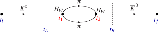
Figure 1: Schematic diagram of the correlation function from which $\Delta m_{K}$ is evaluated. The $K^{0}$ is created at $t_{i}$ and the final-state $\bar{K}^{0}$ is annihilated at $t_{f}$. The times of the two insertions of the weak Hamiltonian are $t_{1,2}$ which are integrated from $t_{A}$ to $t_{B}$. The two-pion intermediate state propagating between $t_{1}$ and $t_{2}$ is drawn for illustration; the calculation includes a sum over all possible intermediate states.

In the lattice calculation we compute the four-point correlation function sketched in Fig. 1. Defining $T=t_{B}-t_{A}+1$ (in lattice units) and integrating the times of the two insertions of the weak Hamiltonian from $t_{A}$ to $t_{B}$ we find

$$C_{4}(t_{A},t_{B};t_{i},t_{f})=|Z_{K}|^{2}e^{-m_{K}(t_{f}-t_{i})}\sum_{n}\,\frac{\langle\bar{K}^{0}\,|\,{H_{W}}\,|\,n\rangle\,\langle n\,|\,{H_{W}}\,|\,K^{0}\rangle}{(m_{K}-E_{n})^{2}}\,\bigg{\{}e^{(m_{K}-E_{n})T}-(m_{K}-E_{n})T-1\bigg{\}}\,,$$ (3)

where the sum is over all allowed intermediate states and $Z_{K}$ is the matrix element of the interpolating operator used to create the $K^{0}$ and annihilate the $\bar{K}^{0}$ between the kaon and the vacuum.

The method proposed in [1] is to identify the coefficient of $T$ from which we obtain:

$$\Delta m_{K}^{\mathrm{FV}}\equiv 2\sum_{n}\,\frac{\langle\bar{K}^{0}\,|\,{H}_{W}\,|\,n\rangle\,\langle n\,|\,{H}_{W}\,|\,K^{0}\rangle}{(m_{K}-E_{n})}\,.$$ (4)

The two-pion energy levels depend on the volume of the lattice. If the volume is tuned so that there is a state, $|n_{0}\rangle$ say, whose energy is equal to $m_{K}$, $E_{n_{0}}=m_{K}$, then from the coefficient of $T$ we obtain instead

$$2\sum_{n\neq n_{0}}\frac{\langle\,\bar{K}\,|\,H_{W}\,|\,n\rangle\,\langle\,n\,|\,H_{W}\,|\,{K}\rangle}{(m_{K}-E_{n})}\,,$$ (5)

(the state $|n_{0}\rangle$ appears in the coefficient of $T^{2}$ and higher powers). The subject of this talk is the evaluation of FV effects necessary to relate the sums in $\Delta m_{K}^{\mathrm{FV}}$ to the corresponding integrals in Eq.(2). This is necessary in order to obtain the physical mass difference from a realistic lattice calculation.

It will be important for the following to note that the correlation function $C_{4}$ itself does not have a pole as the volume is varied so that one of the two-pion energy levels approaches $m_{K}$ (see Eq. (3)). This is not the case however, when one extracts the coefficient of $T$ to obtain $\Delta m_{K}^{\mathrm{FV}}$ (see Eq. (4)).

The discussion here exploits the fact that only two-pion states lies below $m_{K}$ (contributions from three-pion states are neglected) and assumes the dominance of $s$-wave rescattering of the two pions. To simplify the discussion we consider only the dominant $I=0$ contribution; generalising the discussion to include also the $I=2$ channel is straightforward. The relation between the finite-volume sums and infinite-volume integrals for the case in which the volume has been tuned so that there is a state $|n_{0}\rangle$ with $E_{n_{0}}=m_{K}$ was presented by N. Christ at the 2010 Lattice conference [2]. Using degenerate perturbation theory he found

$$\Delta M_{K} = 2\sum_{n\neq n_{0}}\frac{\langle\,\bar{K}\,|\,H_{W}\,|\,n\rangle\,\langle\,n\,|\,H_{W}\,|\,{K}\rangle}{(M_{K}-E_{n})}+\frac{1}{\left(\frac{\partial h}{\partial E}\right)}\Bigg{[}\frac{1}{2}\,\left(\frac{\partial^{2}h}{\partial E^{2}}\right)~{}|\langle n_{0}\,|\,H_{W}\,|\,K_{S}\,\rangle|^{2}$$ (6)

$$\hskip 54.2025pt-\frac{\partial}{\partial E_{n_{0}}}\left\{\left.\frac{\partial h}{\partial E}\right|_{E=E_{n_{0}}}|\langle n_{0}\,|\,H_{W}\,|\,K_{S}\,\rangle|^{2}\right\}_{E_{n_{0}}=M_{K}}\Bigg{]}\,,$$

where $h(E,L)\equiv\phi(q)+\delta(k)$, $\phi$ is a kinematic function defined in [5] and $\delta$ is the $I=0$, $s$-wave phase shift. The Lüscher quantization condition for two-pion states (for $s$-wave dominance) is

$$h(E,L)=n\pi\quad\mathrm{with}\quad E^{2}=4(m^{2}+k^{2})~{}\mathrm{and}~{}q=kL/2\pi\,.$$ (7)

The derivation of Eq. (6) extends the Lellouch-Lüscher method for the derivation of the finite-volume effects in $K\to\pi\pi$ decay amplitudes to next order in degenerate perturbation theory.

The key new result of this study is given in Eq. (21) which suggests a natural strategy for taking the infinite-volume limit. Before presenting this result, we recall some of the salient features of finite-volume effects in the propagation and rescattering of two pions (Sec. 2) and also present a one-dimensional toy example with similar properties to $\Delta m_{K}$ (Sec. 3). The derivation of Eq. (21) is sketched in Sec. 4 where it is also seen that Eq. (6) is a special case. It should be noted however, that we are still developing a complete proof of Eq. (21) and so at this stage it should be considered a well-motivated hypothesis, but given its significance for the evaluation of $\Delta m_{K}$ we present it here.

2 Finite-volume effects for two-pion states

Before proceeding to the discussion of finite-volume effects in the evaluation of $\Delta m_{K}$ it is instructive to recall the derivation of the Lellouch-Lüscher formula [6] using the method of [7]. Consider the correlation function

$$C(t)=\int_{V}d^{3}x~{}~{}\langle\,0\,|\,J(\vec{x},t)\,J(0)\,|\,0\,\rangle=V\sum_{n}\,|\langle\,0\,|\,J(0)\,|\pi\pi,n\,\rangle_{V}|^{2}\,e^{-E_{n}t}\,,$$ (8)

where the suffix $V$ denotes finite-volume matrix elements. As $V\to\infty$, the excitation level at fixed physics becomes large, i.e. $h(E,L)\to\infty$ and the Poisson summation formula implies that

$$\sum_{n}\,f(E_{n})=\int\,dE\,\rho_{V}(E)\,f(E)+\sum_{l\neq 0}\int\,dE\,\rho_{V}(E)\,f(E)\,e^{i2\pi\,l\,h(E,L)}\,,$$ (9)

where

$$\rho_{V}(E)=\frac{dn}{dE}=\frac{q\phi^{\prime}(q)+k\delta^{\prime}(k)}{4\pi k^{2}}\,E\,,$$ (10)

Applying this formula to $C(t)$ we obtain:

$$C(t)\to V\int\,dE\,\rho_{V}(E)\,|\langle\,0\,|\,J(0)\,|\pi\pi,E\,\rangle_{V}|^{2}\,e^{-Et}+\textrm{exponentially small corrections.}$$ (11)

On the other hand, clustering implies that the finite-volume correlation function is equal to the infinite-volume one up to exponentially small corrections so that

$$C(t)=\frac{\pi}{2(2\pi)^{3}}\,\int\,\frac{dE}{E}\,e^{-Et}|\langle\,0\,|\,J(0)\,|\pi\pi,E\,\rangle|^{2}\,k(E)\,,$$ (12)

where $k(E)=\sqrt{E^{2}/4-m^{2}}$. Comparing the expressions in Eqs.(11) and (12), we obtain

$$|\pi\pi,E\rangle=4\pi\sqrt{\frac{VE\rho_{V}(E)}{k(E)}}\,|\pi\pi,E\rangle_{V}\,.$$ (13)

This is the key ingredient of the Lellouch-Lüscher formula, (note also the relation between the normalisations of single-particle states in infinite and finite volumes:
$|K(\vec{p}=0)=\sqrt{2m_{K}V}\,|K(\vec{p}=0)\,\rangle_{V}$).

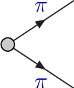
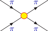
Figure 2: Left - weak vertex which creates two pions from the vacuum. Right - strong vertex leading to the rescattering of two pions.

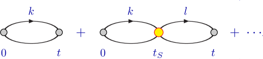
Figure 3: Perturbative contributions to the correlation function.

2.1 Perturbation theory for two-pion states

Note that although $C(t)$ has no non-exponential FV corrections, the energies and matrix elements do. It is instructive to see how this works in perturbation theory. A full calculation for $K\to\pi\pi$ decays in chiral perturbation theory was presented in [8]; here we simplify the calculation while keeping the relevant points. For this illustration consider a weak vertex which can create a two-pion state from the vacuum and a strong-interaction vertex which allows the two pions to rescatter (see Fig. 2).

Evaluating the diagrams in Fig. 3, the correlation function at zero three-momentum is found to be of the form

$$C(t)=\frac{1}{V}\sum_{\vec{k}}\frac{1}{(2\omega_{k})^{2}}e^{-2\omega_{k}t}+\frac{\hat{\lambda}}{V^{2}}\sum_{\vec{k},\vec{l}}\frac{1}{(2\omega_{k})^{2}(2\omega_{l})^{2}}\,\frac{1}{2(\omega_{l}-\omega_{k})}\left\{e^{-2\omega_{k}t}-e^{-2\omega_{l}t}\right\}$$ (14)

where $\omega_{k}^{2}=\vec{k^{2}}+m_{\pi}^{2}$ ($\omega_{l}^{2}=\vec{l^{2}}+m_{\pi}^{2}$) and $\hat{\lambda}$ is proportional to the strong coupling. The starting point for the approach of [7] is that there are no power-like finite-volume corrections in the correlation function and this is manifested by the fact that there is no singularity at $\omega_{k}=\omega_{l}$ in the summand of the second term on the right-hand side of Eq. (14). This does not contradict the fact that, as we know from the pioneering work of Lüscher [5], there are finite-volume corrections to the two-pion energies and, as we know from the Lellouch-Lüscher formula [6], also to the matrix elements. To see this we combine the terms with $|\vec{l}\,|=|\vec{k}\,|$ in the second term on the right-hand side of (14) with the lowest-order contribution to obtain:

$$\frac{1}{V}\sum_{\vec{k}}\frac{1}{(2\omega_{k})^{2}}e^{-2\omega_{k}t}+\frac{\hat{\lambda}}{V^{2}}\sum_{\vec{k}}\frac{\nu_{k}t}{(2\omega_{k})^{4}}\simeq\frac{1}{V}\sum_{\vec{k}}\frac{1}{(2\omega_{k})^{2}}e^{-(2\omega_{k}+\Delta E(k))\,t}\,,$$ (15)

where $\Delta E(k)$ is the finite-volume energy shift as given by Lüscher’s formula. The terms with $|\vec{l}\,|\neq|\vec{k}\,|$ correctly give the Lellouch-Lüscher formula [8]. Sum of the (power-like) finite-volume corrections to the energy and matrix elements cancel as seen in Eq.(14).

The $O(\hat{\lambda})$ term highlighted in Eq. (14) comes from the integral of the time $t_{S}$ at which the strong-vertex in inserted from $0$ to $t$ corresponding to the propagation and rescattering of two pions which are responsible for the power-like finite-volume effects in the energies and matrix elements. The full contribution to the correlation function requires the integral over the complete range of $t_{S}$, the remaining terms do not contain non-exponential finite-volume effects (as demonstrated in [8]).

3 Towards understanding the finite-volume corrections to $\Delta m_{K}$: Some one-dimensional toy examples

An instructive example, with some similar features to the situation encountered in the evaluation of $\Delta m_{K}$ is provided by the one-dimensional formula [9] :

$$\frac{1}{L}\,\sum_{n}~{}\frac{f(p_{n}^{2})}{k^{2}-p_{n}^{2}}={\cal P}\int_{-\infty}^{\infty}\,\frac{dp}{2\pi}~{}\frac{f(p^{2})}{k^{2}-p^{2}}+\frac{f(k^{2})\,\cot(kL/2)}{2k}\,.$$ (16)

The sum on the left-hand side of Eq. (16) is over the integers $n$, with $p_{n}=2\pi n/L$, $L$ is the length of the one-dimensional space and $k$ is an external momentum. $k$ can be considered as being analogous to the relative momentum of each pion in a $K\to\pi\pi$ decay ($m_{K}^{2}=4(m_{\pi}^{2}+k^{2})$). The presence of the pole in the summand on the left-hand side, leads to non-exponential corrections to the difference of the finite-volume sum and infinite-volume integral; these corrections are given by the second term on the right-hand side.

In order to minimise the finite-volume corrections, a sensible strategy would be to tune the volume $L$ such that the $\cot(kL/2)=0$, i.e. $kL=(2n+1)\pi$ where $n$ is an integer (not to be confused with the summation variable). The infinite-volume limit would then be taken (in principle at least), by increasing $L$ while satisfying $\cot(kL/2)=0$, and for each volume only exponentially small finite-volume corrections would be encountered.

An alternative strategy might be to increase the volumes in such a way that at each step $k$ corresponds to one of the allowed momenta, $k=p_{n_{0}}$ say for some integer $n_{0}$ (which increases as the volume is increased). In that case we remove the terms $n=\pm{n_{0}}$ from the sum and find

$$\frac{1}{L}\sum_{n}^{\prime}\frac{f(p_{n}^{2})}{k^{2}-p_{n}^{2}}={\cal P}\int_{-\infty}^{\infty}\,\frac{dp}{2\pi}\,\frac{f(p^{2})}{k^{2}-p^{2}}+\frac{2f^{\prime}(k^{2})}{L}-\frac{f(k^{2})}{2Lk^{2}}\,,$$ (17)

where $f^{\prime}(k^{2})$ indicates the derivative of $f$ w.r.t. $k^{2}$. The ^′ on the sum indicates that the terms with $n=\pm n_{0}$ have been removed. From the right-hand side of Eq. (17) we see explicitly that in this one-dimensional example the power-like finite-volume corrections are $O(1/L)$.

4 Finite-volume effects in $\Delta m_{K}$

Finally we return to $\Delta m_{K}$ and Eq. (3). As already noted, the correlation function $C_{4}$ has no pole as one of the energies $E_{n}\to m_{K}$, and hence no non-exponential finite-volume corrections. However, the proposal in Ref. [1] is to use the $T$-behaviour of $C_{4}$ to extract $\Delta m_{K}^{\mathrm{FV}}$ given in Eq. (4). This does have a pole as $E_{n}\to m_{K}$ and hence non-exponential finite-volume corrections. It is now convenient to make the replacement

$$\frac{1}{m_{K}-E_{n}}\to\frac{m_{K}+E_{n}}{4(k^{2}-p_{n}^{2})}\quad\mathrm{where}\quad m_{K}^{2}\equiv 4(k^{2}+m_{\pi}^{2})~{}\mathrm{and}~{}E_{n}^{2}\equiv 4(p_{n}^{2}+m_{\pi}^{2})\,.$$ (18)

We need to generalise the derivation of Eq. (16), which starts with the relation [10]

$$\frac{1}{L}\,\sum_{n}~{}\frac{f(p_{n}^{2})-f(k^{2})}{k^{2}-p_{n}^{2}}=\int_{-\infty}^{\infty}\,\frac{dp}{2\pi}~{}\frac{f(p^{2})-f(k^{2})}{k^{2}-p^{2}}\,,$$ (19)

where the summand is constructed not to have any poles. Taking

$$f(E_{n})=2\,_{V}\langle\bar{K}^{0}\,|\,{H}_{W}\,|\,n\rangle_{V}\,{}_{V}\langle n\,|\,{H}_{W}\,|\,K^{0}\rangle_{V}\,$$ (20)

and recalling that the quantisation condition is $h(E_{n},L)=n\pi$, we obtain

$$\sum_{n}\frac{f(E_{n})}{m_{K}-E_{n}}={\cal P}\,\int\,dE\,\rho_{V}(E)\,\frac{f(E)}{m_{K}-E}+f(m_{K})\left(\cot(h)\,\frac{dh}{dE}\right)_{\!\!m_{K}}.$$ (21)

The non-exponential finite-volume corrections are contained in the second term on the right-hand side.

Given the result in Eq. (21), what is the best strategy for taking the infinite-volume limit? It appears to be attractive to tune the volumes at each step keeping $\cot(h(m_{K},L))=0$, so that only exponentially small corrections appear. Of course, in practice the tuning will not be perfect and the cotangent term in Eq. (21) allows us to correct for any small mistuning.

From Eq. (21), we can readily obtain the result presented by N.Christ at Lattice 2010 [2]. If we take the infinite-volume limit such that one of the allowed energy levels, $n_{0}$ say, is degenerate with the kaon, $m_{K}=E_{n_{0}}$, then Eq. (21) implies that

$$\sum_{n}\mbox{}^{\prime}\frac{f(E_{n})}{m_{K}-E_{n}}={\cal P}\,\int\,dE\,\rho_{V}(E)\,\frac{f(E)}{m_{K}-E}+f^{\prime}(m_{K})+\frac{1}{2}\,f(m_{K})\,\frac{h^{\prime\prime}}{h^{\prime}}\,.$$ (22)

5 Summary and Conclusions

Progress towards the evaluation of the $K_{L}$ – $K_{S}$ mass difference [1, 4] is one of the examples of the RBC-UKQCD collaboration’s programme of extending the range of physical quantities which can be evaluated in lattice simulations. In order to obtain the physical result from $\Delta m_{K}^{\mathrm{FV}}$ in Eq. (4), determined from the $T$-behaviour of the correlation function, we need to correct for the finite-volume effects which are exhibited in Eqs. (21) and (22).

In this talk we have sketched the derivation of the powerful result in Eq. (21). We are currently working towards a complete proof that threshold effects in $f(E_{n})$ defined in Eq. (20) do not lead to power corrections in the volume. An important consistency check is that Eq. (21) reproduces correctly Eq.(22).

Acknowledgements:

NHC acknowledges partial support from the US DOE grant DE-FG02-92ER40699 and CTS from STFC grant ST/G000557/1.

References

- [1] N. H. Christ, T. Izubuchi, C. T. Sachrajda, A. Soni and J. Yu, Phys. Rev. D 88 (2013) 014508, [arXiv:1212.5931 [hep-lat]].
- [2] N. H. Christ [RBC and UKQCD Collaborations], arXiv:1012.6034 [hep-lat].
- [3] N.H.Christ, these proceedings.
- [4] Jianglei Yu, these proceedings.
- [5] M. Luscher, Nucl. Phys. B 354 (1991) 531.
- [6] L. Lellouch and M. Luscher, Commun. Math. Phys. 219 (2001) 31 [hep-lat/0003023].
- [7] C. J. D. Lin, G. Martinelli, C. T. Sachrajda and M. Testa, Nucl. Phys. B 619 (2001) 467 [hep-lat/0104006].
- [8] C. J. D. Lin, G. Martinelli, E. Pallante, C. T. Sachrajda and G. Villadoro, Nucl. Phys. B 650 (2003) 301 [hep-lat/0208007].
- [9] M. Testa, Lect. Notes Phys. 663 (2005) 177.
- [10] C. h. Kim, C. T. Sachrajda and S. R. Sharpe, Nucl. Phys. B 727 (2005) 218 [hep-lat/0507006].