Constraining Halo Occupation Distribution and Cosmic Growth Rate using Multipole Power Spectrum

Abstract

We propose a new method of measuring halo occupation distribution (HOD) together with cosmic growth rate using multipole components of galaxy power spectrum $P_{l}(k)$. The nonlinear redshift-space distortion due to the random motion of satellite galaxies, i.e., Fingers-of-God, generates high-$l$ multipole anisotropy in galaxy clustering such as the hexadecapole ($l=4$) and tetra-hexadecapole ($l=6$), which are sensitive to the fraction and the velocity dispersion of satellite galaxies. Using simulated samples following the HOD of Luminous Red Galaxies (LRGs), we find that the input HOD parameters are successfully reproduced from $P_{l}(k)$ and that high-$l$ multipole information help to break the degeneracy among HOD parameters. We also show that the measurements of the cosmic growth rate as well as the satellite fraction and velocity dispersions are significantly improved by adding the small-scale information of high-$l$ multipoles.

1 Introduction

Understanding the relationship between galaxy distributions and their host dark matter halos is a key ingredient in the physics of galaxy formation and is also important for precision cosmology study using galaxy datasets. Halo occupation distribution (HOD) describes the probability distribution of the occupation number of central and satellite galaxies as a function of their host halo mass (e.g., Berlind & Weinberg 2002; Berlind et al. 2003; Kravtsov et al. 2004; Zheng et al. 2005). Abundance matching of simulated subhalos to connect the properties of galaxies has been widely investigated (e.g., Masaki et al. 2013). HOD has been measured from a variety of galaxy samples using projected correlation function which is sensitive to the radial profile of galaxies (e.g., Zehavi et al. 2005; Masjedi et al. 2006; Zheng et al. 2009; White et al. 2011; Geach et al. 2012) and also from galaxy group multiplicity functions[e.g.,][]Reid09a. Cross correlation of galaxies with background galaxy image distortions, i.e., galaxy-galaxy lensing, has been measured to connect the halo mass with the galaxy properties (e.g., Mandelbaum et al. 2006). The dilution of the lensing signal around off-centered (satellite) galaxies provides a probe of the satellite fraction and the velocity dispersion (Hikage et al. 2012; George et al. 2012; Hikage et al. 2013).

We propose a novel method to constrain HOD using the multipole galaxy power spectra $P_{l}(k)$ by characterizing the anisotropy of the galaxy clustering due to the redshift-space distortion (RSD). The random motion of galaxies inside their host halos generates the nonlinear redshift-space distortion, i.e., Fingers-of-God (FoG) effect (Jackson 1972). As the off-centered or satellite galaxies have large internal motion, the FoG effect provides a useful probe of constraining the fraction of satellite galaxies. Hikage & Yamamoto (2013) report a clear detection of high-$l$ multipole anisotropy such as hexadecapole ($l=4$) and tetra-hexadecapole ($l=6$), which comes from the FoG effect of one-halo term, the contributions of central-satellite and satellite-satellite pair hosted by the same halos.

In this letter, we utilize such high-$l$ multipole anisotropy to constrain HOD. Focused on the luminous red galaxies (LRGs), which has been widely used for cosmology analysis in SDSS (Eisenstein et al. 2001), we construct simulated mock LRG samples on the HOD basis. We show that the input HOD is reproduced from $P_{l}(k)$. High-$l$ multipole is sensitive to satellite velocity distribution, while the projected correlation function depends on the radial profile of satellite galaxies in the host halos. Both measurements play complimentary roles in understanding the relationship between galaxies and halos.

The bulk motion of galaxies drives the anisotropy in galaxy clustering, which provides a powerful observational probe of measuring the cosmic growth rate to test General Relativity and various gravity models (Peacock et al. 2001; Okumura et al. 2008; Guzzo et al. 2008). Combinations of monopole ($l=0$) and quadrupole ($l=2$) power spectra has been widely used to constrain growth rate from various galaxy samples including SDSS LRG (Yamamoto et al. 2008, 2010; Sato et al. 2011; Oka et al. 2013) and recently BOSS CMASS sample (Reid et al. 2012; Beutler et al. 2013; Samushia et al. 2013). Satellite FoG effect is a major systematic uncertainty in measuring the growth rate in this analysis. Even when the satellite fraction of the SDSS LRG sample is just 6%, the measurement of growth rate can be strongly biased (Hikage & Yamamoto 2013). As high-$l$ multipole spectra such as $P_{4}$ and $P_{6}$ are sensitive to the satellite fraction, they are useful for eliminating the uncertainty of the satellite FoG. In this letter, we show that the measurement of growth rate as well as HOD parameters is significantly improved by adding high-$l$ multipole information.

This letter is organized as follows: in section 2, we present the theoretical formalism to describe the multipole power spectra based on the halo model. In section 3, we summarize how to make simulation data for LRG catalogs. The results of the measurements of HOD and the growth rate are summarized in section 4. Section 5 is devoted to summary and conclusions. Throughout the letter, we use flat $\Lambda$ CDM model with the fiducial cosmological parameters as follows: $\Omega_{b}h^{2}=0.0226$, $\Omega_{c}h^{2}=0.1108$, $n_{s}=0.963$, $h=0.704$, $\tau=0.089$, $\sigma_{8}=0.817$.

2 Formalism

In this section, we summarize our theoretical formulae of the multipole power spectra of LRGs based in the HOD framework.

2.1 Multipole power spectra in halo model

Galaxy power spectrum in redshift space $P(k,\mu)$, where $\mu$ is the cosine of the angle between the wavevector $\mathbf{k}$ and the line-of-sight direction, is described by expanding their multipole components:

$$P_{l}(k)=\frac{2l+1}{2}\int_{-1}^{1}d\mu P(k,\mu){\cal L}_{l}(\mu),$$ (1)

where ${\cal L}_{l}$ is $l$-th Legendre polynomials. In the halo-model approach (e.g., Seljak 2000; White 2001; Cooray & Sheth 2002), the galaxy power spectrum can be decomposed into the one-halo and two-halo terms,

$$P(k,\mu)=P^{\rm 1h}(k,\mu)+P^{\rm 2h}(k,\mu).$$ (2)

One-halo term is the contribution from the clustering of central-satellite and satellite-satellite pairs hosted by same halos and written as follows:

$$P^{\rm 1h}(k,\mu) = \frac{\displaystyle 1}{\displaystyle n_{\rm tot}^{2}}\int dM\frac{dn_{\rm h}}{dM}\Bigl{[}2\langle N_{\rm cen}N_{\rm sat}\rangle\tilde{p}_{\rm sat}(k,\mu;M)$$ (3)

$$+\langle N_{\rm sat}(N_{\rm sat}-1)\rangle\tilde{p}_{\rm sat}^{2}(k,\mu;M)\Bigr{]},$$

where $dn_{\rm h}/dM$ is the halo mass function, $\langle N_{\rm cen}\rangle$ and $\langle N_{\rm sat}\rangle$ denote the HOD of central and satellite galaxies respectively, $n_{\rm tot}$ is the total number density of galaxies (see the details of HOD parametrization in the next subsection). Here we assume that the halo hosting satellite LRGs must have a central LRG and thereby $\langle N_{\rm cen}N_{\rm sat}\rangle=\langle N_{\rm sat}\rangle$ (Zheng et al. 2005). This assumption is good for our purpose, though some of central galaxies are not always LRGs (e.g., Skibba et al. 2011). We assume that the occupation number of satellite galaxies follows Poisson statistics, which implies $\langle N_{\rm sat}(N_{\rm sat}-1)\rangle=\langle N_{\rm sat}\rangle^{2}$ (Kravtsov et al. 2004; Zehavi et al. 2005). We neglect the velocity dispersion of central galaxies. The satellite distribution around central galaxies inside the halo with mass $M$ is described with $\tilde{p}_{\rm sat}(k,\mu;M)$. We consider that the radial profile of satellite galaxies follows the NFW profile (Navarro et al. 1997) with the concentration given by Duffy et al. (2008) and the internal velocity of satellite galaxies has Gaussian distribution

$$\tilde{p}_{\rm sat}(k,\mu,M) = \tilde{u}_{\rm NFW}(k;M)\exp\left[-\frac{\sigma_{v}^{\rm(vir)2}(M)k^{2}\mu^{2}}{2a^{2}H^{2}(z)}\right].$$ (4)

where $\tilde{u}_{\rm NFW}(k)$ is the Fourier transform of the NFW density profile. The velocity dispersion of satellite galaxies is given by the Virial velocity dispersion $\sigma_{v}^{\rm(vir)}\equiv(GM/2r_{\rm vir})^{1/2}$ and then the average velocity dispersion of satellite galaxies is given using the satellite HOD as

$$\sigma_{v}^{\rm(sat)}=\left[\frac{1}{n_{\rm sat}}\int dM\frac{dn_{\rm h}}{dM}\langle N_{\rm sat}\rangle\sigma_{v}^{\rm(vir)2}\right]^{1/2},$$ (5)

where $n_{\rm sat}$ is the number density of satellite galaxies. The satellite fraction $f_{\rm sat}$ is defined as $n_{\rm sat}/n_{\rm tot}$.

The two-halo term, which is the contribution of the clustering of LRGs in different halos, depends on the redshift-space halo power spectra with different halo masses $P_{\rm hh}(k;M,M^{\prime})$ (Hikage et al. 2013):

$$P^{\rm 2h}(k,\mu)=\frac{\displaystyle 1}{\displaystyle n_{\rm tot}^{2}}\int dM\frac{\displaystyle dn_{\rm h}}{\displaystyle dM}\int dM^{\prime}\frac{\displaystyle dn_{\rm h}}{\displaystyle dM^{\prime}}~{}~{}~{}~{}~{}~{}~{}~{}~{}~{}~{}~{}~{}~{}~{}~{}~{}~{}~{}~{}~{}~{}~{}~{}~{}~{}~{}$$

$$\times\left[\langle N_{\rm cen}\rangle+\langle N_{\rm sat}\rangle\tilde{p}_{\rm sat}(k,\mu;M)\right]~{}~{}~{}~{}~{}~{}~{}~{}~{}~{}~{}~{}~{}~{}~{}~{}~{}~{}~{}~{}~{}~{}~{}$$

$$\times\left[\langle N_{\rm cen}\rangle+\langle N_{\rm sat}\rangle\tilde{p}_{\rm sat}(k,\mu;M^{\prime})\right]P_{\rm hh}(k,\mu;M,M^{\prime}).$$ (6)

The two-halo term is also affected by FoG effect of satellite galaxies while the internal motion of central galaxy is assumed to be negligible. We directly estimate the redshift-space halo power spectra $P_{\rm hh}(k,\mu;M,M^{\prime})$ using simulations to incorporate various nonlinear effects such as the gravitational evolution, the halo biasing, and the halo motion. We divide the simulated halo samples into 10 different mass bins to compute their auto- and cross-halo power spectra in redshift space (see section 3 for details).

2.2 Parametrization of Halo Occupation Distribution (HOD)

We consider two different ways to describe HOD of central and satellite LRGs.

1. One is using a following functional form of HOD (Zheng et al. 2005):

   $$\langle N_{\rm cen}\rangle = \frac{1}{2}\left[1+{\rm erf}\left(\frac{\log_{10}(M)-\log_{10}(M_{\rm min})}{\sigma_{\log M}}\right)\right],$$

   $$\langle N_{\rm sat}\rangle = \langle N_{\rm cen}\rangle\left(\frac{M-M_{\rm cut}}{M_{1}}\right)^{\alpha},$$ (7)

   where ${\rm erf}(x)$ is the error function and five HOD parameters are included. The fiducial values of the HOD parameters for SDSS DR7 LRG sample is set as $M_{\rm min}=5.7\times 10^{13}h^{-1}M_{\odot}$, $\sigma_{\log M}=0.7$, $M_{\rm cut}=3.5\times 10^{13}h^{-1}M_{\odot}$, $M_{1}=3.5\times 10^{14}h^{-1}M_{\odot}$, and $\alpha=1$ (Reid & Spergel 2009).

2. The other way is not assuming any functional form of HOD. We parametrize central and satellite HODs at different mass and interpolate the HOD of intermediate halo mass with cubic spline approximation. We divide 5 different mass bins (10 HOD parameters in total) in the mass range from $10^{12}h^{-1}M_{\odot}$ to $10^{15}h^{-1}M_{\odot}$. We assume that the satellite number $\langle N_{\rm sat}\rangle$ monotonically increases as larger halo mass $M$.

3 Simulation with the HOD of LRGs

We construct simulated samples with the HOD of LRGs to estimate the error of HOD parameters and growth rate from the measurements of $P_{l}$. We run 100 realizations of N-body simulations using Gadget-2 code (Springel 2005). The initial distribution of mass particles is set using 2LPT code in Gaussian initial condition (Crocce et al. 2006) with the initial redshift of $z=49$. The initial matter power spectrum is computed using CAMB software (Lewis et al. 2000) with the fiducial cosmological parameters. The N-body simulations are performed in a periodic cubic box at the side length $L_{\rm box}$ of $1h^{-1}$Gpc with the number of mass particles is 800³ where each particle mass is $1.3\times 10^{11}h^{-1}M_{\odot}$. Halo is identified by Friends-of-Friends algorithm with the linking length $b=0.2$. The minimum number of mass particles constituting halos is 20, which corresponds to the halo mass of $2.6\times 10^{12}h^{-1}M_{\odot}$. The position and velocity of each halo is defined as the arithmetic mean of those of the constituent mass particles of each halo.

We randomly select halos hosting a central LRG and pick up the dark matter particles for satellite LRGs to follow the fiducial HOD (eqs. [7,8]). The number distribution of satellite LRGs follow Poisson statistics. The position and velocity of the host halo and the mass particles are respectively assigned to those of central and satellite LRGs. In the fiducial HOD values, the fraction of satellite LRGs is 6.5% and their average velocity dispersion $\sigma_{v}^{\rm(sat)}$ is $570$km/s in average. For simplicity, the simulations do not include various observational issues such as the angular mask, radial selection function, and fiber collisions.

Number density is assigned to each grid with the nearest grid point (NGP) scheme and the number of grids $N_{\rm grid}$ is set to be 512 at a side. We compute the multipole power spectrum by transforming the density field into Fourier space with Fast Fourier Transform (FFT) method. The shot noise term, the inverse of the number density in the sample, is subtracted from the monopole power spectrum. The covariance of the multipole power spectra $P_{l}$ at different $l$ and different bins of $k$ is estimated from 100 realizations of simulated samples. We also combine jackknife resampling method and obtain the enough number of realizations to estimate the covariance.

We take z-axis as the line-of-sight direction and obtain the redshift-space position by adding the velocity component $v_{z}$

$$s=r+\frac{f_{z}}{f_{z}^{\rm(GR)}}\frac{(1+z)v_{z}}{H(z)}.$$ (8)

In order to estimate the deviation of the growth rate $f_{z}$ from the GR prediction $f_{z}^{\rm(GR)}$, we simply change the amplitude of velocity by hand (c.f., Nishimichi & Oka 2013). We compute the halo power spectrum for $f_{z}=(1\pm\Delta)f_{z}^{\rm(GR)}$ with $\Delta=0.1$ and linearly interpolate them to estimate $P_{\rm hh}$ for arbitrary $f_{z}$ in the theoretical model (eq.[6]). For simplicity, we neglect the change of the halo mass function and the halo bias from their GR prediction.

4 Results

4.1 Satellite FoG effects on multipole power spectra

Figure 1 shows the simulation results of $P_{4}$ and $P_{6}$ (black circles) in comparison with the model predictions with the same HOD (black lines). They are found to be in excellent agreement with each other. For comparison, we plot the model predictions by varying the satellite fraction $f_{\rm sat}$ and the satellite velocity dispersion $\sigma_{v}^{\rm(sat)}$. High-$l$ multipoles, which is mainly determined by the one-halo term, are sensitive to the satellite properties through their velocity distribution or FoG effect. As the satellite fraction is small for the LRG sample, central-satellite pair contribution is dominant and thus the overall amplitude of $P_{l}$ ($l\geq 4$) is roughly proportional to $f_{\rm sat}$ (see eq.[3]). As $\sigma_{v}^{\rm(sat)}$ increases, the FoG effect starts at smaller $k$ while the overall amplitude of $kP_{l}^{1h}$ at large-$k$ limit decreases (Hikage & Yamamoto 2013). The feature can be seen especially in $P_{4}$ in the lower panels of Figure 1.

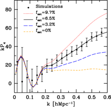
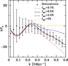
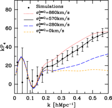
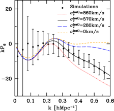
Figure 1: Hexadecapole $P_{4}(k)$ (left) and tetra-hexadecapole $P_{6}(k)$ (right) for the mock LRG samples in average (black circles). Error-bars denote the 1-$\sigma$ dispersion. The black lines represent the model prediction with the fiducial values of HOD in which the satellite fraction is $f_{\rm sat}=6.5$% and the satellite velocity dispersion is $\sigma_{v}^{\rm(sat)}=570$km/s. For comparison, we plot the theoretical models by varying $f_{\rm sat}$ (Upper) and $\sigma_{v}^{\rm(sat)}$ (Lower). The binning width $\Delta k$ for these plots is $0.032h$/Mpc, which is twice larger than that in the fitting.

		$\sigma_{8}$, $\delta N$ fixed						$\sigma_{8}$, $\delta N$ free
parameters	input	$P_{0,2}(k\leq 0.2)$	$P_{0,2}(k\leq 0.2)$	$P_{0,2}(k\leq 0.2)$	$P_{0,2}(k\leq 0.6)$	$P_{0,2}(k\leq 0.6)$		$P_{0,2}(k\leq 0.6)$	$P_{0,2}(k\leq 0.6)$
	values	–	$P_{4}(k\leq 0.6)$	$P_{4,6}(k\leq 0.6)$	–	$P_{4,6}(k\leq 0.6)$		–	$P_{4,6}(k\leq 0.6)$
$M_{\rm min}$	5.7	$5.28\pm 0.36$	$5.47\pm 0.23$	$5.45\pm 0.22$	$5.54\pm 0.11$	$5.54\pm 0.11$		$6.37\pm 0.91$	$5.52\pm 0.79$
$\sigma_{\log M}$	0.7	$0.66\pm 0.04$	$0.68\pm 0.02$	$0.68\pm 0.02$	$0.68\pm 0.01$	$0.68\pm 0.01$		$0.76\pm 0.14$	$0.68\pm 0.07$
$M_{\rm cut}$	3.5	$6.2\pm 4.1$	$4.8\pm 2.4$	$4.4\pm 2.4$	$1.4\pm 1.7$	$3.4\pm 1.4$		$6.4\pm 3.4$	$3.8\pm 2.0$
$M_{1}$	35	$35\pm 13$	$34\pm 6$	$34\pm 5$	$37\pm 3$	$35\pm 2.2$		$35\pm 7$	$34\pm 2.9$
$\alpha$	1	$0.96\pm 0.26$	$0.90\pm 0.21$	$0.94\pm 0.21$	$1.04\pm 0.20$	$1.02\pm 0.19$		$0.84\pm 0.24$	$1.01\pm 0.22$
$\chi^{2}_{\rm min}$ (d.o.f.)	–	0.2 (20)	1.7 (57)	2.2 (94)	1.0 (70)	2.9 (144)		0.88 (68)	2.8 (142)

Table 1: The best-fit values of HOD parameters in the functional form (eq.[7]) measured from different combinations of $P_{l}$ for $k\leq 0.2$ or $0.6h$/Mpc ($l=0,2$) and $k\leq 0.6h$/Mpc ($l=4,6$) averaged over 100 simulated samples. Cosmological parameters are fixed except for the rightmost two columns, which shows the results including $\sigma_{8}$ and the residual shot noise $\delta N$ as additional free parameters. The input values of HOD parameters are listed for reference. The error is estimated using the covariance of $P_{l}$ at different $l$ and bins of $k$ for 1($h^{-1}$Gpc)³ boxes. The minimum chi-square values $\chi^{2}_{\rm min}$ in the fitting and the degree-of-freedom (d.o.f.) in parentheses are also listed. The unit of mass is $10^{13}h^{-1}M_{\odot}$.

4.2 Reconstructions of HOD from multipole power spectra

We apply Markov Chain Monte Carlo method to the averaged simulated power spectra over 100 realizations to estimate the likelihood function of a parameter set $\mathbf{p}$ in the chi-square basis:

$$\chi^{2} = \sum_{i,j}[y_{i}^{\rm(model)}(\mathbf{p})-y_{i}^{\rm(sim)}]{\rm Cov}^{-1}_{ij}[y_{j}^{\rm(model)}(\mathbf{p})-y_{j}^{\rm(sim)}]$$ (9)

$$+[(N_{\rm tot}^{\rm(sim)}-N_{\rm tot}^{\rm(model)})/\sigma_{N}]^{2},$$

where $y_{i}$ denotes $P_{l}(k)$ at each $l$ and bin of $k$, $\mathbf{p}$ include HOD parameters and the growth rate, and Cov denotes the covariance of $P_{l}(k)$ for 1($h^{-1}$Gpc)³ boxes. The second term on the right-hand side represents the constraint on the total number of LRGs including both central and satellite LRGs. We give the error of $N_{\rm tot}$ as $\sigma_{N}=\sqrt{N_{\rm tot}}$.

Table 1 lists the best-fit values and the 1$\sigma$ errors of the five HOD parameters in the functional form (eq.[7]). The binning width $\Delta k$ is set to be $0.016h$/Mpc and then the number of bins are 12 ($k\leq 0.2h$/Mpc) and 37 ($k\leq 0.6h$/Mpc) for each $P_{l}$. When the information of $P_{0}$ and $P_{2}$ is included up to $k=0.2h$/Mpc, where the perturbation theory agrees with the simulations (Beutler et al. 2013), the addition of the small-scale information of $P_{4}$ and $P_{6}$ reduces the error of HOD parameters by nearly half. When the information of $P_{0}$ and $P_{2}$ up to $k=0.6h$/Mpc as same as $P_{4}$ and $P_{6}$ are included, the improvement by adding $P_{4}$ and $P_{6}$ is 20-30% for the satellite HOD parameters of $M_{\rm cut}$ and $M_{1}$. When varying the amplitude of matter power spectrum ($\sigma_{8}$) and the residual shot noise $\delta N$ as additional free parameters, the constraints only from $P_{0}$ and $P_{2}$ becomes much weaker due to the degeneracy between the two-halo term and the one-halo term. The information of $P_{4}$ and $P_{6}$, which mainly determined by the one-halo term, helps to break the degeneracy and significantly improve the HOD constraints.

Figure 2 shows the reconstructed HOD from $P_{l}$ of the simulated LRG samples when the functional form of HOD is assumed (upper panels) and when central and satellite HOD values is directly fitted without assuming any functional form of HODs (lower panels). The reconstructed HODs agree with the input HOD (lines) within the 1-sigma error in both cases and the addition of high-$l$ multipole improve the HOD measurements as shown by the light-blue shaded area in upper panel.

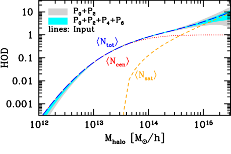
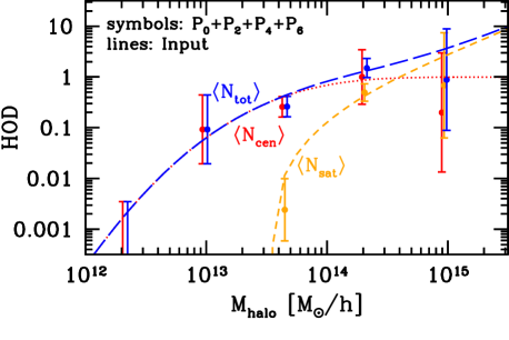
Figure 2: Reconstructed HOD by fitting HOD parameters to $P_{l}(k)$ for the simulated LRG catalog. Upper panel shows the result when the functional form of HOD (eq. [7]) is assumed. Shaded area denote the 1-$\sigma$ error of $\langle N_{\rm tot}\rangle$ from $P_{0}$ and $P_{2}$ (Gray area) and $P_{0},P_{2},P_{4}$ and $P_{6}$ (light blue area). For reference, the input HOD for total (blue), central (red), and satellite galaxies (yellow) are plotted. Lower panel shows the result when central and satellite HOD values at 5 different mass bins are directly measured without assuming any functional form using $P_{0}$, $P_{2}$, $P_{4}$ and $P_{6}$. The error-bars denote the 1-$\sigma$ error.

4.3 Constraints on the growth rate

Fingers-of-God effect due to satellite galaxies is a major systematic uncertainty in measuring the cosmic growth rate. High-$l$ multipoles sensitive to the satellite properties improve the accuracy of growth rate measurement (Hikage & Yamamoto 2013). Table 2 shows the constraints on the satellite fraction $f_{\rm sat}$ and the average velocity dispersion $\sigma_{v}^{\rm(sat)}$ when using a functional form of HOD and direct fitting of HOD values at 5 different bins of mass. Note that $\sigma_{v}^{\rm(sat)}$ is determined by the HOD values using the Virial theorem (eq.[5]). We find that addition of $P_{4}$ and $P_{6}$ improve the measurement of the growth rate by nearly twice (the error decreases from 8% to 4%) in both of the HOD parametrization.

Figure 3 shows the joint constraints on the fraction of satellite galaxies $f_{\rm sat}$ and the growth rate index $\gamma$, which is calculated with the simple approximation $f_{z}=\Omega_{m}^{\gamma}(z)$, and the satellite velocity dispersion $\sigma_{v}^{\rm(sat)}$ from different combinations of $P_{l}$. The parameters $f_{\rm sat}$ and $f_{z}$ degenerate with each other because the suppression of quadrupole power due to satellite FoG effect is mimicked by increasing the growth rate $f_{z}$ (or decreasing $\gamma$). Figure 3 shows that the addition of high-$l$ multipole measurements breaks their degeneracy and then improves the accuracy of $\gamma$ by nearly twice. The input values denoted by the cross symbols are successfully reproduced.

parameters	input	$P_{0},P_{2}$	$P_{0},P_{2},P_{4}$	$P_{0},P_{2},P_{4},P_{6}$
HOD (5 parameter models in the functional form of eq. 7)
$100f_{\rm sat}$	6.5	$5.7\pm 1.2$	$6.4\pm 0.7$	$6.4\pm 0.7$
$\sigma_{v}^{\rm(sat)}$ [km/s]	570	$604\pm 46$	$570\pm 29$	$569\pm 25$
$f_{z}/f_{z}^{\rm GR}$	1	$1.01\pm 0.09$	$1.01\pm 0.06$	$1.01\pm 0.05$
$\gamma$	0.545	$0.53\pm 0.12$	$0.53\pm 0.08$	$0.53\pm 0.07$
HOD (direct fitting of $\langle N_{\rm cen}\rangle$ and $\langle N_{\rm sat}\rangle$ at 5 mass bins)
$100f_{\rm sat}$	6.5	$5.9\pm 1.6$	$6.0\pm 0.8$	$6.2\pm 0.7$
$\sigma_{v}^{\rm(sat)}$ [km/s]	570	$583\pm 86$	$556\pm 40$	$571\pm 26$
$f_{z}/f_{z}^{\rm GR}$	1	$1.03\pm 0.09$	$1.03\pm 0.06$	$1.01\pm 0.05$
$\gamma$	0.545	$0.51\pm 0.12$	$0.51\pm 0.08$	$0.53\pm 0.07$

Table 2: Constraints on the satellite fraction $f_{\rm sat}$, the satellite velocity dispersion $\sigma_{v}^{\rm(sat)}$, the growth rate normalized by the GR predictions $f_{z}/f_{z}^{\rm GR}$ and the growth rate index $\gamma$ from different combinations of $P_{l}$. We use $k\leq 0.2$ for $P_{0}$ and $P_{2}$ and $k\leq 0.6$ for $P_{4}$ and $P_{6}$. We show the case when using a functional form of HOD in the equation 7 (Upper) and when fitting central and satellite HOD values at 5 different bins of halo mass as free parameters but assuming that $\langle N_{\rm sat}\rangle$ increases as larger $M$ (Lower).

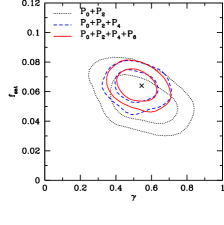
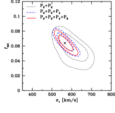
Figure 3: Joint constraints on the satellite fraction $f_{\rm sat}$ and the growth rate index $\gamma$ (left) or $\sigma_{v}^{\rm(sat)}$ (right) from $P_{0}+P_{2}$ (black), $P_{0}+P_{2}+P_{4}$ (blue), and $P_{0}+P_{2}+P_{4}+P_{6}$ (red). Here we use a functional form of HOD (eq [7]). Each contour denotes 68% and 95% error respectively. The symbol of crosses denote the input values.

5 Summary and Conclusions

We present the HOD constraints from multipole galaxy power spectra $P_{l}(k)$ using the simulated catalogs which follows HOD of SDSS LRG samples. The high-$l$ multipole spectra such as $P_{4}$ and $P_{6}$ are sensitive to the Fingers-of-God (FoG) effect due to the large internal motion of satellite galaxies and thus they are useful probe to constrain the fraction and the velocity dispersion of satellite galaxies. We find that the input HOD is successfully reconstructed from $P_{l}$ and that high-$l$ multipole spectra significantly improve the accuracy of the HOD measurements. We also find that the addition of high-$l$ multipole information improve the accuracy of the growth rate measurement by nearly twice because they break the degeneracy between the cosmic growth rate and the satellite FoG.

In this letter we simply use the simulated samples in $1(h^{-1}{\rm Gpc})^{3}$ cubic box. To apply our method for the actual observations, we need to consider the various observational issues such as the angular mask, radial selection function and the fiber collision. Such observational effect can be evaluated by making the mock samples with the same geometry as the observation. Various methods to correct the fiber collision effect has been also developed (e.g., Guo et al. 2012). We also need to consider the uncertainty of cosmology and halo power spectra more exactly. The uncertainty mainly affect $P_{0}$ and $P_{2}$ where the two-halo term is dominant, while high-$l$ multipole power spectra dominated by the one-halo term are insensitive to the details of the halo power spectrum. Even when fitting cosmology parameters together with HOD parameters, high-$l$ multipole spectra should be still important to eliminate the satellite FoG effect. Measuring the deviation of the satellite velocity dispersion from the virial velocity dispersion provides useful information related to the satellite kinematics (e.g., Tinker 2007). These works are beyond the scope of this letter and left for the future.

References

- Berlind & Weinberg (2002) Berlind A. A., Weinberg D. H., 2002, ApJ, 575, 587
- Berlind et al. (2003) Berlind A. A. et al., 2003, ApJ, 593, 1
- Beutler et al. (2013) Beutler F. et al., 2013, ArXiv e-prints
- Cooray & Sheth (2002) Cooray A., Sheth R., 2002, Physics Report, 372, 1
- Crocce et al. (2006) Crocce M., Pueblas S., Scoccimarro R., 2006, MNRAS, 373, 369
- Duffy et al. (2008) Duffy A. R., Schaye J., Kay S. T., Dalla Vecchia C., 2008, MNRAS, 390, L64
- Eisenstein et al. (2001) Eisenstein D. J. et al., 2001, AJ, 122, 2267
- Geach et al. (2012) Geach J. E., Sobral D., Hickox R. C., Wake D. A., Smail I., Best P. N., Baugh C. M., Stott J. P., 2012, MNRAS, 426, 679
- George et al. (2012) George M. R. et al., 2012, ApJ, 757, 2
- Guo et al. (2012) Guo H., Zehavi I., Zheng Z., 2012, ApJ, 756, 127
- Guzzo et al. (2008) Guzzo L., et al., 2008, Nature, 451, 541
- Hikage et al. (2013) Hikage C., Mandelbaum R., Takada M., Spergel D. N., 2013, MNRAS, 435, 2345
- Hikage et al. (2012) Hikage C., Takada M., Spergel D. N., 2012, MNRAS, 419, 3457
- Hikage & Yamamoto (2013) Hikage C., Yamamoto K., 2013, JCAP, 8, 19
- Jackson (1972) Jackson J. C., 1972, MNRAS, 156, 1P
- Kravtsov et al. (2004) Kravtsov A. V., Berlind A. A., Wechsler R. H., Klypin A. A., Gottlöber S., Allgood B., Primack J. R., 2004, ApJ, 609, 35
- Lewis et al. (2000) Lewis A., Challinor A., Lasenby A., 2000, ApJ, 538, 473
- Mandelbaum et al. (2006) Mandelbaum R., Seljak U., Kauffmann G., Hirata C. M., Brinkmann J., 2006, MNRAS, 368, 715
- Masaki et al. (2013) Masaki S., Lin Y.-T., Yoshida N., 2013, MNRAS, 436, 2286
- Masjedi et al. (2006) Masjedi M. et al., 2006, ApJ, 644, 54
- Navarro et al. (1997) Navarro J. F., Frenk C. S., White S. D. M., 1997, ApJ, 490, 493
- Nishimichi & Oka (2013) Nishimichi T., Oka A., 2013, ArXiv e-prints
- Oka et al. (2013) Oka A., Saito S., Nishimichi T., Taruya A., Yamamoto K., 2013, ArXiv e-prints
- Okumura et al. (2008) Okumura T., Matsubara T., Eisenstein D. J., Kayo I., Hikage C., Szalay A. S., Schneider D. P., 2008, ApJ, 676, 889
- Peacock et al. (2001) Peacock J. A., et al., 2001, Nature, 410, 169
- Reid et al. (2012) Reid B. A. et al., 2012, MNRAS, 426, 2719
- Reid & Spergel (2009) Reid B. A., Spergel D. N., 2009, ApJ, 698, 143
- Samushia et al. (2013) Samushia L. et al., 2013, ArXiv e-prints
- Sato et al. (2011) Sato T., Hütsi G., Yamamoto K., 2011, Progress of Theoretical Physics, 125, 187
- Seljak (2000) Seljak U., 2000, MNRAS, 318, 203
- Skibba et al. (2011) Skibba R. A., van den Bosch F. C., Yang X., More S., Mo H., Fontanot F., 2011, MNRAS, 410, 417
- Springel (2005) Springel V., 2005, MNRAS, 364, 1105
- Tinker (2007) Tinker J. L., 2007, MNRAS, 374, 477
- White (2001) White M., 2001, MNRAS, 321, 1
- White et al. (2011) White M. et al., 2011, ApJ, 728, 126
- Yamamoto et al. (2010) Yamamoto K., Nakamura G., Hütsi G., Narikawa T., Sato T., 2010, Phys. Rev. D, 81, 103517
- Yamamoto et al. (2008) Yamamoto K., Sato T., Hütsi G., 2008, Progress of Theoretical Physics, 120, 609
- Zehavi et al. (2005) Zehavi I. et al., 2005, ApJ, 630, 1
- Zheng et al. (2009) Zheng Z., Zehavi I., Eisenstein D. J., Weinberg D. H., Jing Y. P., 2009, ApJ, 707, 554
- Zheng et al. (2005) Zheng Z., et al., 2005, ApJ, 633, 791