Application of canonical Hamiltonian formulation to nonlinear light-envelope propagations

Abstract

We first point out it is conditional to apply the variational approach to the nonlocal nonlinear Schrödinger equation (NNLSE), that is, the response function must be an even function. Different from the variational approach, the canonical Hamiltonian formulation for the first-order differential system are used to deal with the problems of the nonlinear light-envelope propagations. The Hamiltonian of the system modeled by the NNLSE is obtained, which can be expressed as the sum of the generalized kinetic energy and the generalized potential. The solitons correspond to extreme points of the generalized potential. The stabilities of solitons in both local and nonlocal nonlinear media are also investigated by the analysis of the generalized potential. They are stable when the potential has minimum, and unstable otherwise.

.

I Introduction

The Hamiltonian viewpoint provides a framework for theoretical extensions in many areas of physics Goldstein-book-05 ; menon-EJP ; Maschke-IEEE ; Escobar-Automatica ; Buchdahl-book-93 . In classical mechanics it forms the basis for further developments, such as Hamilton-Jacobi theory, perturbation approaches and chaos. The canonical equations of Hamilton in classical mechanics are of the form

$$\dot{q_{i}}=\frac{\partial H}{\partial p_{i}},-\dot{p_{i}}=\frac{\partial H}{\partial q_{i}},\quad(i=1,\cdots,n),$$ (1)

where $q_{i}$ and $p_{i}$ are said to be the generalized coordinate and the generalized momentum, $\dot{q}_{i}=dq_{i}/dt$, $\dot{p}_{i}=dp_{i}/dt$, and $H$ is the Hamiltonian. There are many situations in which the Hamiltonian is equal to the sum of the generalized kinetic energy $T$ and the generalized potential $V$. The conditions are that the generalized potential is not a function of generalized velocities, and the generalized kinetic energy is a homogeneous quadratic function of generalized velocities. Once the generalized potential $V$, which is under the framework of the Hamiltonian system, is obtained, the problem of the small oscillations of a system about positions of equilibrium can be easily dealt with. For a conservative mechanical system its equilibrium state can be obtained by $\left(\frac{\partial V}{\partial q_{i}}\right)_{0}=0.$ The generalized potential has an extremum at the equilibrium configuration of the system, which is marked with the subscript $0$. The equilibrium is stable when the extremum of the potential $V$ is the minimum, and unstable otherwise.

Up to now, to our knowledge, the canonical equations of Hamilton appearing in all the literatures are of the form (1) except for our recent work, where it is pointed out that the canonical equations of Hamilton (1) are only valid for the second-order differential system (the system described by the second-order partial differential equation about the evolution coordinate) but not valid for the first-order differential system (the system described by the first-order partial differential equation about the evolution coordinate). The nonlinear Schrödinger equation (NLSE) is the first-order differential system, which is a universal nonlinear model that describes many nonlinear physical systems and can be applied to hydrodynamics Nore-Physica D-93 , nonlinear optics Anderson-pra-83 , nonlinear acoustics Bisyarin-AIP Conf. Proc.-08 , Bose-Einstein condensates seaman-pra-05 , and so on. The work about the canonical equations of Hamilton for the first-order differential system will be introduced briefly here.

The approximate analytical solutions of the NLSE can be obtained by the variational approach Anderson-pra-83 ; Hasegawa-apl-73 ; Anderson-josab-1988 ; Malomed-progress in optics-2002 , where the light-envelope is treated as the classical particle traveling in an equivalent potential, whose minimum corresponds to the soliton. In this paper we use the canonical equations of Hamilton to deal with the nonlinear light-envelope propagations. Such an approach is different from the the variational approach, which will be illustrated in the paper. We can divide the Hamiltonian of the system into the generalized kinetic energy and the generalized potential, the extreme point of which corresponds to the soliton. But in some other literatures Seghete-pra-2007 ; Picozzi-prl-2011 ; Lashkin-pla-2007 ; Petroski-oc-2007 , solitons are regarded as the extrema of the Hamiltonian of the system. Such a treatment has some problems, which will be illustrated in the paper. To determine the stabilities of the soliton, we can determine whether the generalized potential has a minimum. Solitons are stable when the generalized potential has a minimum, but unstable otherwise. In fact, the similar expression, the Hamiltonian expressed as the sum of the generalized kinetic energy and the generalized potential, appeared in Ref.Desyatnikov-prl-10 , but the elaboration of the systematic theoretical principle was absent, which is often of great importance.

The paper is organized as follows. In Sec. II, we briefly introduce the model, the nonlocal nonlinear Schrödinger equation (NNLSE). The restriction on the the response function in the the variational approach is discussed in Sec. III, we point out the variational approach can be used to find the approximately analytical solution of the NNLSE if and only if the response function is an even function. We use the canonical equations to deal with the nonlinear light-envelope propagations in the paper, but the conventional canonical equations of Hamilton are not valid for NNLSE, so in Sec. IV we will briefly introduce the canonical equations of Hamilton valid for the first-order differential system, which will be reported elsewhere in detail. The application of the canonical equations of Hamilton introduced in Sec. IV to the NNLSE is shown in Sec. V. By use of the canonical equations of Hamilton, we can find the soliton solutions of the NNLSE, and can analyze the stability characteristics of the solitons. The difference between the variational approach and the approach employed in the paper is discussed in Sec. VI. Sec. VII gives the summary.

II Model

The propagation of the light-envelope in the nonlocal cubic nonlinear media is modeled by the nonlocal nonlinear Schrödinger equation (NNLSE) in the dimensionless system  Snyder-science-97 ; Mitchell-josab-99 ; Krolikowski-pre-01 ; Conti-prl-10

$$i\frac{\partial\varphi}{\partial z}+\Delta_{\bot}\varphi+\varphi\int_{-\infty}^{\infty}R(\textbf{r}-\textbf{r}^{\prime})|\varphi(\textbf{r}^{\prime},z)|^{2}d^{D}\textbf{r}^{\prime}=0,$$ (2)

where $\varphi(r,z)$ is the complex amplitude envelop, $z$ is the longitudinal coordinate, r and $\textbf{r}^{\prime}$ are the $D$-dimensional transverse coordinate vectors. $d^{D}\textbf{r}^{\prime}$ is a $D$-dimensional volume element at $\textbf{r}^{\prime}$, $\Delta_{\bot}$ is the $D$-dimensional transverse Laplacian operator, and $R$ is normalized response function of the media such that $\int_{-\infty}^{\infty}R(\textbf{r}^{\prime})d^{D}\textbf{r}^{\prime}=1$. For a singular response, i.e., $R(\textbf{r})=\delta(\textbf{r})$, Eq.(2) simplifies to the NLSE

$$i\frac{\partial\varphi}{\partial z}+\Delta_{\bot}\varphi+|\varphi|^{2}\varphi=0.$$ (3)

When $D=1$, NNLSE (2) can describe the propagations of both optical beams Snyder-science-97 ; Mitchell-josab-99 ; Krolikowski-pre-01 and pulses Conti-prl-10 . Particularly, it was predicted very recently Conti-prl-10 that strongly nonlocal temporal solitons can exist in the model (2). The second term of (2) models the diffraction for the optical beam, and the group velocity dispersion (GVD) Agrawal-book-01 for the optical pulse. The nonlinear term of (2) describes the self focusing of the optical beam Chiao-prl-64 and optical pulse Hasegawa-apl-73 . Generally speaking, when $D=2$, NNLSE (2) only describes the propagations of optical beams. The propagation of a pulsed optical beam can be described by the NNLSE, and a optical bullet Silberberg-ol-90 can be obtained when $D=3$. For $D>3$, the NNLSE (2) is just a phenomenological model, the counterpart of which can not be found in physics. The response function $R$ can be symmetric for the optical beam, but is asymmetric for the optical pulse due to the causality Boyd-book-92 .

III Discussion about the variational approach for the nonlocal nonlinear Schrödinger equation

To find the approximately analytical solution of the NNLSE, the variational approach is widely used Guo-oc-06 . The reason that the variational approach can be applied to the NNLSE is that the NNLSE can be viewed as the Euler-Lagrange equation

$$\frac{\partial}{\partial z}\frac{\partial l}{\partial\left(\frac{\partial\varphi^{*}}{\partial z}\right)}+\frac{\partial}{\partial x}\frac{\partial l}{\partial\left(\frac{\partial\varphi^{*}}{\partial x}\right)}-\frac{\partial l}{\partial\varphi^{*}}=0,$$ (4)

where $l$ is the Lagrangian density. Replacing $\varphi^{*}$ with $\varphi$, the complex-conjugate equation of the NNLSE can be obtained from the Euler-Lagrange equation (4). It is easy to calculate the first two terms of Eq. (4), but is some difficult to calculate the last term because of the convolution between the response function and the intensity of the optical beam for the NNLSE. In the following we will take the NNLSE (2) with $D=1$ as an example to discuss the condition under which the NNLSE (2) is equivalent to the Euler-Lagrange equation (4).

The Lagrangian density of the NNLSE (2) is Guo-oc-06

$$l=\frac{i}{2}\left(\varphi^{*}\frac{\partial\varphi}{\partial z}-\varphi\frac{\partial\varphi^{*}}{\partial z}\right)-\left|\frac{\partial\varphi}{\partial x}\right|^{2}+\frac{1}{2}\left|\varphi(x,z)\right|^{2}\Delta n,$$ (5)

where $\Delta n=\int_{-\infty}^{\infty}R(\textbf{r}-\textbf{r}^{\prime})\left|\varphi(\textbf{r}^{\prime},z)\right|^{2}d^{D}\textbf{r}^{\prime}$. Inserting the Lagrangian density (5) into the Euler-Lagrange equation (4), the first two terms of (4) can be easily obtained as

$$\frac{\partial}{\partial x}\frac{\partial l}{\partial\left(\frac{\partial\varphi^{*}}{\partial x}\right)}+\frac{\partial}{\partial z}\frac{\partial l}{\partial\left(\frac{\partial\varphi^{*}}{\partial z}\right)}=i\frac{\partial\varphi}{\partial z}+\frac{\partial^{2}\varphi}{\partial x^{2}}.$$ (6)

To calculate the last term, we first construct a functional by integrating the last term of the Lagrangian density (5) as

$$F(\varphi,\varphi^{*})=\frac{1}{2}\int_{-\infty}^{\infty}\Delta n(x)|\varphi(x)|^{2}dx=\frac{1}{2}\int_{-\infty}^{\infty}\int_{-\infty}^{\infty}R(x-x^{\prime})|\varphi(x^{\prime})|^{2}|\varphi(x)|^{2}dx^{\prime}.$$ (7)

The variation of the functional $F(\varphi,\varphi^{*})$ can be obtained by definition as

$$\delta F(\varphi,\varphi^{*}) = \frac{\partial}{\partial\varepsilon}F(\varphi+\varepsilon\delta\varphi,\varphi^{*}+\varepsilon\delta\varphi^{*})|_{\varepsilon\rightarrow 0}$$ (8)

$$= \frac{1}{2}\int_{-\infty}^{\infty}\int_{-\infty}^{\infty}R(x-x^{\prime})|\varphi(x)|^{2}\left[\varphi(x^{\prime})\delta\varphi^{*}(x^{\prime})+\varphi^{*}(x^{\prime})\delta\varphi(x^{\prime})\right]dx^{\prime}dx$$

$$+\frac{1}{2}\int_{-\infty}^{\infty}\Delta n\left[\varphi(x)\delta\varphi^{*}(x)+\varphi^{*}(x)\delta\varphi(x)\right]dx.$$

If the response function is a even function, i.e., $R(x)=R(-x)$, then we can obtain that $\int_{-\infty}^{\infty}\int_{-\infty}^{\infty}R(x-x^{\prime})|\varphi(x)|^{2}\left[\varphi(x^{\prime})\delta\varphi^{*}(x^{\prime})+\varphi^{*}(x^{\prime})\delta\varphi(x^{\prime})\right]dx^{\prime}dx=\int_{-\infty}^{\infty}\Delta n\left[\varphi(x)\delta\varphi^{*}(x)+\varphi^{*}(x)\delta\varphi(x)\right]dx$. Then the variation of the functional $F(\varphi,\varphi^{*})$ is simplified to

$$\delta F(\varphi,\varphi^{*})=\int_{-\infty}^{\infty}\Delta n\varphi(x)\delta\varphi^{*}(x)dx+\int_{-\infty}^{\infty}\Delta n\varphi^{*}(x)\delta\varphi(x)dx.$$ (9)

Because the variation of the functional $F(\varphi,\varphi^{*})$ can be also expressed as

$$\delta F(\varphi,\varphi^{*})=\int_{-\infty}^{\infty}\frac{\partial}{\partial\varphi}\left[\frac{1}{2}\Delta n(x)|\varphi(x)|^{2}\right]\delta\varphi(x)dx+\int_{-\infty}^{\infty}\frac{\partial}{\partial\varphi^{*}}\left[\frac{1}{2}\Delta n(x)|\varphi(x)|^{2}\right]\delta\varphi^{*}(x)dx.$$ (10)

Comparing Eq.(9) and (10), we obtain

$$\frac{\partial}{\partial\varphi^{*}}\left[\frac{1}{2}\Delta n(x)|\varphi(x)|^{2}\right] = \Delta n\varphi(x),$$ (11)

$$\frac{\partial}{\partial\varphi}\left[\frac{1}{2}\Delta n(x)|\varphi(x)|^{2}\right] = \Delta n\varphi^{*}(x).$$ (12)

Then the NNLSE (2) can be obtained from the Euler-Lagrange equation (4) by combining Eq.(6) and Eq.(11), its complex-conjugate equation can be obtained by combining Eq.(6) and Eq.(12).

Consequently, it is conditional to apply the variational approach to the NNLSE, that is, the response function must be an even function. When the response function is not an even function, the variational approach will do not work any longer.

IV Canonical equations of Hamilton for the first-order differential system

We will use the canonical equations of Hamilton to deal with the nonlinear light-envelope propagations. However the canonical equations of Hamilton appearing in all the literatures, except for our recent work, are only valid for the second-order differential system but not valid for the first-order differential system while the NNLSE (2) is the first-order differential system. Therefore, it is necessary to briefly introduce the canonical equations of Hamilton for the first-order differential system first.

For the first-order differential system of the continuous systems, the Lagrangian density must be the linear function of the generalized velocities, and expressed as

$$l=\sum_{s=1}^{N}R_{s}(q_{s})\dot{q}_{s}+Q(q_{s},q_{s,x}),$$ (13)

where $R_{s}$ is not the function of a set of $q_{s,x}$. Consequently, the generalized momentum $p_{s}$, which is obtained by the definition $p_{s}=\partial l/\partial\dot{q}_{s}$ as

$$p_{s}=R_{s}(q_{s}),(s=1,\cdots,N)$$ (14)

is only a function of $q_{s}$. There are $2N$ variables, $q_{s}$ and $p_{s}$, in Eqs. (14). The number of Eqs. (14) is $N$, which also means there exist $N$ constraints between $q_{s}$ and $p_{s}$. So the degree of freedom of the system given by Eqs. (14) is $N$. Without loss of generality, we take $q_{1},\cdots,q_{\nu}$ and $p_{1},\cdots,p_{\mu}$ as the independent variables, where $\nu+\mu=N$. The remaining generalized coordinates and generalized momenta can be expressed with these independent variables as $q_{\alpha}=q_{\alpha}(q_{1},\cdots,q_{\nu},p_{1},\cdots,p_{\mu})(\alpha=\nu+1,\cdots,N),$ and $p_{\beta}=p_{\beta}(q_{1},\cdots,q_{\nu},p_{1},\cdots,p_{\mu})(\beta=\mu+1,\cdots,N).$ The Hamiltonian density $h$ for the continuous system is obtained by the Legendre transformation as $h=\sum_{s=1}^{N}\dot{q}_{s}p_{s}-l$, where the Hamiltonian density $h$ is a function of $\nu$ generalized coordinates, $q_{1},\cdots,q_{\nu}$, and $\mu$ generalized momenta, $p_{1},\cdots,p_{\mu}$. We can obtain $N$ canonical equations of Hamilton

$$\frac{\delta h}{\delta q_{\lambda}} = \sum_{s=1}^{N}\left(\dot{q}_{s}\frac{\partial p_{s}}{\partial q_{\lambda}}-\dot{p}_{s}\frac{\partial q_{s}}{\partial q_{\lambda}}\right)+\sum_{\alpha=\nu+1}^{N}\frac{\partial}{\partial x}\frac{\partial h}{\partial q_{\alpha,x}}\frac{\partial f_{\alpha}}{\partial q_{\lambda}},$$ (15)

$$\frac{\delta h}{\delta p_{\eta}} = \sum_{s=1}^{N}\left(\dot{q}_{s}\frac{\partial p_{s}}{\partial p_{\eta}}-\dot{p}_{s}\frac{\partial q_{s}}{\partial p_{\eta}}\right)+\sum_{\alpha=\nu+1}^{N}\frac{\partial}{\partial x}\frac{\partial h}{\partial q_{\alpha,x}}\frac{\partial f_{\alpha}}{\partial p_{\eta}}$$ (16)

($\lambda=1,\cdots,\nu$, $\eta=1,\cdots,\mu$, and $\nu+\mu=N$). The canonical equations of Hamilton (15) and (16) can be easily extended to the discrete system, which can be expressed as

$$\frac{\partial H}{\partial q_{\lambda}} = \sum_{s=1}^{N}\left(\dot{q}_{s}\frac{\partial p_{s}}{\partial q_{\lambda}}-\dot{p}_{s}\frac{\partial q_{s}}{\partial q_{\lambda}}\right),$$ (17)

$$\frac{\partial H}{\partial p_{\eta}} = \sum_{s=1}^{N}\left(\dot{q}_{s}\frac{\partial p_{s}}{\partial p_{\eta}}-\dot{p}_{s}\frac{\partial q_{s}}{\partial p_{\eta}}\right),$$ (18)

where $\lambda=1,\cdots,\nu$, $\eta=1,\cdots,\mu$, and $\nu+\mu=N$.

V Application in nonlinear light-envelope propagations

Before the application of the canonical equations of Hamilton (17) and (18), we should firstly calculate the Hamiltonian by the Legendre transformation reading $H=\sum_{s=1}^{N}\dot{q}_{s}p_{s}-L$, where the Lagrangian $L$ can be obtained as $L=\int_{-\infty}^{\infty}ld^{D}\textbf{r}.$ The Lagrangian $L$ is a function of generalized coordinates, $\varphi,\varphi^{*}$ and generalized velocities, $\dot{\varphi},\dot{\varphi}^{*}$. It is clear that the Lagrangian is not an explicit function of $z$, so the Hamiltonian of the system is conservative. Now, we assume the light-envelop has a given form, $\varphi=\varphi\left(q_{1},\cdots,q_{n}\right)$, where $q_{1},\cdots,q_{n}$ are the parameters changing with $z$. It can be regarded as the variables transformation, with which we transform the coordinate system expressed by the set of generalized coordinate $\varphi$ to the one expressed by another set of generalized coordinates $q_{1},\cdots,q_{n}$.

Here we assume the material response is the Gaussian function $R(\textbf{r})=\frac{1}{(\sqrt{\pi}w_{m})^{D}}\exp\left(-\frac{|\textbf{r}|^{2}}{w_{m}^{2}}\right),$ and the trial solution has the form, $\varphi(r,z)=q_{A}(z)\exp\left[-\frac{r^{2}}{q_{w}^{2}(z)}\right]\exp\left[iq_{c}(z)r^{2}+iq_{\theta}(z)\right],$ where $q_{A},q_{\theta}$ are the amplitude and phase of the complex amplitude of the light-envelope, respectively, $q_{w}$ is the width of the light-envelope, $q_{c}$ is the phase-front curvature, and they all vary with the propagation distance $z$. We obtain the Lagrangian

$$L = -2^{-2-D}\pi^{D/2}q_{A}^{2}q_{w}^{-2+D}(w_{m}^{2}+q_{w}^{2})^{-D/2}$$ (19)

$$[-2q_{A}^{2}q_{w}^{2+D}+2^{D/2}(w_{m}^{2}+q_{w}^{2})^{D/2}(4D$$

$$+4Dq_{c}^{2}q_{w}^{4}+Dq_{w}^{4}\dot{q}_{c}+4q_{w}^{2}\dot{q}_{\theta})],$$

which is a function of generalized coordinates, $q_{A},q_{w},q_{c}$ and generalized velocities, $\dot{q}_{c},\dot{q}_{\theta}$, but not an explicit function of $z$. The generalized momenta can be obtained

$$p_{A} = p_{w}=0,$$ (20)

$$p_{c} = -2^{-2-\frac{D}{2}}D\pi^{D/2}q_{A}^{2}q_{w}^{2+D},$$ (21)

$$p_{\theta} = -\left(\frac{\pi}{2}\right)^{D/2}q_{A}^{2}q_{w}^{D}.$$ (22)

The Hamiltonian of the system then can be determined by Legendre transformation

$$H = 2^{-1-D}\pi^{D/2}q_{A}^{2}q_{w}^{-2+D}(w_{m}^{2}+q_{w}^{2})^{-D/2}[-q_{A}^{2}q_{w}^{2+D}$$ (23)

$$+2^{1+\frac{D}{2}}D(w_{m}^{2}+q_{w}^{2})^{D/2}(1+q_{c}^{2}q_{w}^{4})],$$

and can be proved to be a constant, i.e. $\dot{H}=0.$

There are four generalized coordinates and four generalized momenta in the four equations (20)(21)(22). So the degree of freedom of the set of equations (20)(21)(22) is four. Without loss of generality, we take $q_{c},q_{\theta},p_{c}$ and $p_{\theta}$ as the independent variables. From Eqs.(21)(22), the generalized coordinates $q_{A},q_{w}$ can be expressed by generalized momenta $p_{c}$ and $p_{\theta}$ as $q_{A}=(-p_{\theta})^{1/2}[Dp_{\theta}/(2\pi p_{c})]^{D/4},q_{w}=[4p_{c}/(Dp_{\theta})]^{1/2},$ inserting which into the Hamiltonian (23), we have

$$H=-\frac{D^{2}p_{\theta}^{2}+16p_{c}^{2}q_{c}^{2}}{4p_{c}}-\frac{1}{2}\pi^{-D/2}(\frac{4p_{c}}{Dp_{\theta}}+w_{m}^{2})^{-D/2}.$$ (24)

By use of the canonical equations of Hamilton (17) and (18), where $\mu=\nu=2$ and $n=4$, we can obtain the following four equations

$$\dot{q}_{c} = \frac{D^{2}p_{\theta}^{2}}{4p_{c}^{2}}-4q_{c}^{2}+\frac{D\pi^{-D/2}p_{\theta}^{2}(\frac{4p_{c}}{Dp_{\theta}}+w_{m}^{2})^{-D/2}}{4p_{c}+Dp_{\theta}w_{m}^{2}},$$ (25)

$$\dot{q}_{\theta} = -\frac{(4+D)\pi^{-D/2}p_{c}p_{\theta}(\frac{4p_{c}}{Dp_{\theta}}+w_{m}^{2}){}^{-D/2}}{4p_{c}+Dp_{\theta}w_{m}^{2}}$$ (26)

$$-\frac{D^{2}p_{\theta}}{2p_{c}}-\frac{D\pi^{-D/2}p_{\theta}^{2}w_{m}^{2}(\frac{4p_{c}}{Dp_{\theta}}+w_{m}^{2}){}^{-D/2}}{4p_{c}+Dp_{\theta}w_{m}^{2}},$$

$$\dot{p}_{c} = 8p_{c}q_{c},$$ (27)

$$\dot{p}_{\theta} = 0.$$ (28)

Because $q_{\theta}$ is a cyclic coordinate, the corresponding generalized momentum $p_{\theta}$ is a constant, which can be confirmed by Eq.(28). In fact, this also represents that the power of the light-envelope, $P_{0}=\int_{-\infty}^{\infty}\left|\varphi\right|^{2}d^{D}\textbf{r}=q_{A}^{2}(\sqrt{\pi/2}q_{w})^{D}$, is conservative. From this we can obtain

$$q_{A}^{2}=P_{0}(\sqrt{\pi/2}q_{w})^{-D}.$$ (29)

Taking the derivative with respect to $z$ on both sides of Eq.(21), then comparing it with Eq.(27), we can obtain with the aid of Eq.(29)

$$q_{c}=\frac{\dot{q}_{w}}{4q_{w}}.$$ (30)

Then inserting Eq.(30) into the Hamiltonian (23) with the aid of Eq.(29), we have $H=T+V,$ where

$$T = \frac{1}{16}DP_{0}\dot{q}_{w}^{2},$$ (31)

$$V = \frac{DP_{0}}{q_{w}{}^{2}}-\frac{1}{2}\pi^{-D/2}P_{0}^{2}\left(w_{m}^{2}+q_{w}{}^{2}\right){}^{-D/2}.$$ (32)

For the system, there are only one independent generalized coordinate $q_{w}$ and one independent generalized velocity $\dot{q}_{w}$, which can be proved in the Appendix. When the Hamiltonian is expressed with independent variables, it is indeed the total energy expressed as the sum of the generalized kinetic energy and the generalized potential.

The problem associated with the NNSLE is a problem of small oscillations from the Hamiltonian point of view. The soliton corresponds to the extremum point of the generalized potential. But in some literatures Seghete-pra-2007 ; Picozzi-prl-2011 ; Lashkin-pla-2007 ; Petroski-oc-2007 , solitons were regarded as the extrema of the Hamiltonian. Such a treatment has some problem, because in those literatures the trial solution has a changeless profile (solitonic profile), the system expressed with the solitonic profile is the static system. The kinetic energy of the static system is zero, and the Hamiltonian is equal to the potential of the static system. In this connection, the extremum of the Hamiltonian is the extremum of the generalized potential of the static system. But when the system deviates from the equilibrium, the extremum of the Hamiltonian is not the extremum of the generalized potential.

From $\partial V/\partial q_{w}=0$, we have

$$-\frac{32}{q_{w}^{3}}+8\pi^{-D/2}P_{0}q_{w}\left(w_{m}^{2}+q_{w}^{2}\right)^{-1-\frac{D}{2}}=0.$$ (33)

From Eq.(33) we can easily obtain the critical power, with which the light-envelope will propagate with a changeless shape. Here we take the notation $P_{c}$ to denote the critical power instead of $P_{0}$, then we obtain

$$P_{c}=\frac{4\pi^{D/2}\left(w_{m}^{2}+q_{w}^{2}\right)^{1+\frac{D}{2}}}{q_{w}^{4}}.$$ (34)

When $P_{0}=P_{c}$, we can obtain that $\dot{q}_{c}=q_{c}=0,$ which implies that the wavefront of the soliton solution is a plane. The propagation constant is $\dot{q}_{\theta}=[(4-D)q_{w}^{2}+4w_{m}^{2}]/q_{w}^{4}$.

Then we elucidate the stability characteristics of the soliton by means of the analysis of the generalized potential $V$. Performing the second-order derivative of the generalized potential $V$ with respect to $q_{w}$, then inserting the critical power into it, we obtain

$$\Upsilon\equiv\left.\frac{\partial^{2}V}{\partial q_{w}^{2}}\right|_{P_{0}=P_{c}}=\frac{64}{q_{w}^{4}}\left[2-\frac{2+D}{2\left(1+\sigma^{2}\right)}\right],$$ (35)

where $\sigma=w_{m}/q_{w}$ is the degree of nonlocality. The larger is $\sigma$, the stronger is the degree of nonlocality. When $\Upsilon>0$, the generalized potential has a minimum, and the soliton is stable. From Eq.(35) we can obtain the criterion of the stability of solitons, that is

$$\sigma^{2}>\frac{1}{4}(D-2),$$ (36)

which is, in fact, consistent with the Vakhitov-Kolokolov (VK) criterion Vakhitov-qe-75 with the aid of the results of Ref.Bang-pre-02 , and is proved briefly in prove .

V.1 The local case

When $w_{m}\rightarrow 0$, the response function $R(\textbf{r})\rightarrow\delta(\textbf{r})$. The NNLSE will be reduced to the NLSE (3). Eqs. (34) and (35) are transformed to

$$P_{c}=4\pi^{D/2}q_{w}^{D-2},\Upsilon=\frac{32}{q_{w}^{4}}(2-D).$$ (37)

When $D=1$, $P_{c}=4\sqrt{\pi}/q_{w}$, which is consistent with Eq.(42) of Ref. Anderson-pra-83 . When $D=2$, $P_{c}=4\pi$, which is the same as Eq.(16a) of Ref. Desaix-josab-91 . We can obtain $\Upsilon>0$ when $D<2$, $\Upsilon<0$ when $D>2$, and $\Upsilon=0$ when $D=2$. So for the local case, the soliton is stable for (1+1)-dimensional case, but unstable when $D>2$. It needs the further analysis for $D=2$ because $\Upsilon=0.$ When $D=2$, the potential (32) is deduced to

$$V=\frac{\left(4\pi-P_{0}\right)P_{0}}{2\pi q_{w}^{2}},$$ (38)

which has no extreme when $P_{0}\neq 4\pi$. When $P_{0}=p_{c}=4\pi$, $V=0$, which is the extreme but not the minimum. So the (1+2)-dimensional local solitons are unstable. The relation between the potential $V$ and the width $q_{w}$ of the light-envelope is shown in Fig.1. If the power of the light-envelope equals to the critical power, the potential will be a constant, as can be seen by dash curve of Fig.(1). Without the external disturbance, the light-envelope will stay in its initial state, and keep its width changeless. If the external disturbance makes the power larger than the critical power, then the width will become more and more smaller, and collapses at last, as can be confirmed by the dash-dot curve of Fig.1. If the external disturbance makes the power smaller than the critical power, then the width will become more and more larger, and diffracts at last, as can be confirmed by the solid curve of Fig.1. These conclusions are consist with those of Refs. Berge-PR-98 ; Moll-prl-03 ; sun-oe-08 .

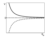
Figure 1: Qualitative plot of the potential $V$ as a function of $q_{w}$ for three cases, $P_{0}<P_{c}$ (solid curve), $P_{0}=P_{c}$ (dashed curve), and $P_{0}>P_{c}$ (dash-dot curve) when $D=2$.

V.2 The nonlocal case

For the nonlocal case, when $D\leq 2$, the condition (36) can be satisfied automatically. That is to say the (1+1)-dimensional and the (1+2)-dimensional nonlocal solitons are always stable when the response function of the material is a Gaussian function. It is consistent with the conclusion of Ref. Bang-pre-02 . When $D>2$ the solitons can be stable only if the criterion of the stability Eq.(36) should be satisfied first, which is also the same as the result of Ref.Bang-pre-02 .

VI differences from the variational approach

The method employed in the paper, based on the Hamiltonian formulation, is different from the widely used variational approach. The first difference is that the equations obtained by the two approaches are different. The equations obtained by the variational approach are the differential equations Anderson-pra-83 . But the equation we obtained is just a simple algebraic equation by differentiating the generalized potential with respect to the generalized coordinates. The other difference is that the ”potentials” obtained by the two approaches are very different. The potential obtained by the variational approach Anderson-pra-83 is just an equivalent potential, which is obtained by comparing the evolution of the width of the light-envelope with the motion of a particle in a potential well. But in the paper, the potential we obtained is the potential from the Hamiltonian point of view.

VII Conclusion

We point out the variational approach can be used to find the approximately analytical solution of the NNLSE if and only if the response function is an even function. We apply the canonical Hamiltonian formulation to nonlinear light-envelope propagations. The Hamiltonian of the nonlinear system can be expressed as the sum of the generalized kinetic energy and the generalized potential. Solitons correspond to the extreme of the generalized potential. Solitons are stable when the generalized potential has the minimum, and unstable otherwise.

APPENDIX. Proof of a proposition

If the Lagrangian of a system is expressed as $L(q_{1},\cdots,q_{j-1},q_{j+s},\cdots,q_{n},\dot{q}_{1},\cdots,\dot{q}_{i-1},\dot{q}_{i+m},\cdots,\dot{q}_{n})$, where $m$ generalized velocities, $\dot{q}_{i},\dot{q}_{i+1},\cdots,\dot{q}_{i+m-1}$, and $s$ generalized coordinates, $q_{j},q_{j+1},\cdots,q_{j+s-1}$, are both not included, then the system only has $n-m-s$ independent variables($n-m-s$ independent generalized coordinates and $n-m-s$ independent generalized velocities).

Inserting the cyclic coordinates, $q_{j},q_{j+1},\cdots,q_{j+s-1}$, into the Euler-Lagrange equations (LABEL:EulerLag) and replacing $t$ with $z$, we have $\frac{d}{dz}\left(\frac{\partial L}{\partial\dot{q}_{\nu}}\right)=0,\ (\alpha=1,\cdots,s),$ i.e.

$$\frac{\partial L}{\partial\dot{q}_{\alpha}}=C_{\alpha},$$ (39)

where $C_{\alpha}$ is a constant independent of $z$. Because NNLSE is a first-order differential equation, the Lagrangian of the system (19) is a function of the first degree in $\dot{q}_{\nu}$, then from Eq.(39), we have the following $s$ constraints

$$f_{\alpha}(q_{1},\cdots,q_{j-1},q_{j+s},\cdots,q_{n})=0,$$ (40)

where $f_{\alpha}=\partial L/\partial\dot{q_{\alpha}}-C_{\alpha}$. Form the Euler-Lagrange equations associated with the disappearing generalized velocities, $\dot{q}_{i},\dot{q}_{i+1},\cdots,\dot{q}_{i+m-1}$, we obtain another $m$ constraints

$$g_{\beta}(q_{1},\cdots,q_{j-1},q_{j+s},\cdots,q_{n},\dot{q}_{1},\cdots,\dot{q}_{i-1},\dot{q}_{i+m},\cdots,\dot{q}_{n})\\ =0,$$

where $g_{\beta}=\partial L/\partial q_{\beta}$ and $\beta=1,\cdots,m.$ The remaining generalized coordinates and generalized velocities of the Lagrangian appear in pairs. They satisfy the differential equations

$$J_{\gamma}(q_{1},\cdots,q_{j-1},q_{j+s},\cdots,q_{n},\dot{q}_{1},\cdots,\dot{q}_{i-1},\dot{q}_{i+m},\cdots,\dot{q}_{n})=0,$$ (41)

where $J_{\gamma}=\frac{d}{dz}(\frac{\partial L}{\partial\dot{q}_{\gamma}})-\frac{\partial L}{\partial q_{\gamma}}$ and $\gamma=1,\cdots,n-m-s$. Taking the derivative with respect to $z$ on both sides of Eq.(40), we have

$$F_{\alpha}(q_{1},\cdots,q_{j-1},q_{j+s},\cdots,q_{n},\dot{q}_{1},\cdots,\dot{q}_{j-1},\dot{q}_{j+s},\cdots,\dot{q}_{n})=0,$$

where $F_{\alpha}=\sum_{\iota}\frac{\partial f_{\alpha}}{\partial q_{\iota}}\dot{q}_{\iota}$, and $\iota=1,\cdots,j-1,j+s,\cdots,n.$ Any $s$ generalized velocities in the function $F_{\alpha}$ can be expressed with the remaining generalized velocities and all generalized coordinates appearing in $F_{\alpha}$. Inserting the $s$ generalized velocities into the differential equations (41), then there are only $n-m-s$ independent generalized velocities appearing in (41). In a similar way, any $m$ generalized coordinates in the function $g_{\nu}$ can be expressed with the remaining generalized coordinates and all generalized velocities appearing in $g_{\nu}$. Inserting the $m$ generalized coordinates into the differential equations (41), then there are only $n-m-s$ independent generalized coordinates appearing in (41). Accordingly, there are only $n-m-s$ generalized coordinates and $n-m-s$ generalized velocities for the system.

References

- (1) H. Goldstein, C. Poole and J. Safko, Classical Mechanics(3rd ed, Higher Education Press, 2005), pp.34-36,238-241,334-349.
- (2) V.J. Menon and D.C. Agrawal, Eur. J. Phys. 16 80 (1995)
- (3) B.M. Maschke, A.J. van der Schaft, and P.C. Breedveld, IEEE Trans. Circuits Systems, 42(2), 73 (1995).
- (4) G. Escobar, A.J. van der Schaft, and R. Ortega, Automatica, 35, 445 (1999).
- (5) Buchdahl, An Introduction to Hamiltonian Optics(Dover Publications, 1993).
- (6) C. Nore, M.E. Brachet, and S. Fauve, Physica D 65, 154 (1993).
- (7) D. Anderson, Phys. Rev. A27, 3135 (1983).
- (8) M. A. Bisyarin, AIP Conf. Proc. 1022, 38-41 (2008).
- (9) B.T. Seaman, L.D. Carr, and M.J. Holland, Phys. Rev. A71 033622 (2005).
- (10) A. Hasegawa and F. Tappert, Appl. Phys. Lett. 23, 142 (1973).
- (11) D. Anderson, M. Lisak, and T. Reichel, J. Opt. Soc. Am. B, 5, 207 (1988).
- (12) B.A. Malomed, in Progress in optics, edited by E. Wolf (North-Holland, 2002), vol.43, pp.71-193.
- (13) V. Seghete, C.R. Menyuk and B.S. Marks, Phys. Rev. A 76, 043803 (2007).
- (14) A. Picozzi and J. Garnier, Phys. Rev. Lett. 107, 233901 (2011).
- (15) V.M. Lashkin, A.I. Yakimenkoa, and O.O. Prikhodko, Phys. Lett. A 366, 422 (2007).
- (16) M.M. Petroski, M.S. Petrović, M.R. Belić, Opt.Commun. 279,196 (2007).
- (17) A.S.Desyatnikov, D.Buccoliero, M.R.Dennis and Y.S.Kivshar, Phys. Rev. Lett 104 053902 (2010).
- (18) A.W. Snyder and D.J. Mitchell, Science 276, 1538 (1997)
- (19) D.J. Mitchell and A.W. Snyder, J. Opt. Soc. Am. B 16, 236 (1999)
- (20) W. Krolikowski et al., Phys. Rev. E 64, 016612 (2001)
- (21) C. Conti, M. A.Schmidt, P. St.J.Russell, and F. Biancalana, Phys. Rev. Lett. 105, 263902 (2010)
- (22) G.P. Agrawal, Nonlinear Fiber Optics, 3rd ed. (Acadamic, San Diego, CA, 2001)
- (23) R. Y. Chiao, E. Garmire, and C. H. Townes, Phys. Rev. Lett. , 13, 479 (1964).
- (24) Y. Silberberg, Opt. Lett. , 15, 1282 (1990).
- (25) R.W. Boyd, Nonlinear Optics (Academic Press, San Diego, CA, 1992).
- (26) Q. Guo, B. Luo, and S. Chi, Opt. Commun. 259, 336 (2006).
- (27) N. G. Vakhitov and A. A. Kolokolov, Radiophys. Quantum Electron. 16, 783 (1975).
- (28) O. Bang, W. Krolikowski, J. Wyller, and J. J. Rasmussen, Phys. Rev. E 66, 046619 (2002).
- (29) To avoid confusion, we make the notations used in Ref.Bang-pre-02 consistent with those in the paper, where we use and to represent the width of the response function and the light-envelope instead of , respectively. In Ref.Bang-pre-02 , , with and , where is the soliton power, and is the propagation constant of solitons. According to the VK criterion, when the soliton become linearly stable. We can derive from the VK criterion , where represents the degree of nonlocality.
- (30) M. Desaix, D. Anderson, and M. Lisak, J. Opt. Soc. Am. B8, 2082 (1991).
- (31) L. Berge. Phys. Rep. 303, 259 (1998)
- (32) K. D. Moll, A. L. Gaeta, and G. Fibich, Phys. Rev. Lett. 90 203902 (2003)
- (33) C. Sun, C. Barsi, and J. W. Fleischer, Opt. Express 16 20676 (2008)