Lepton Polarization Asymmetries of $H\to\gamma\tau^{+}\tau^{-}$ Decays in Standard Model

Abstract

Recently, CMS and ATLAS collaborations at LHC announced a Higgs like particle with mass near $125$GeV. Regarding this, to explore its intrinsic properties, different observables are needed to be measured precisely at the LHC for various decay channels of the Higgs. In this context, we calculate the final state lepton polarization asymmetries, namely, single lepton polarization asymmetries ($P_{i}$) and double lepton polarization asymmetries ($P_{ij}$) in the SM for radiative semileptonic Higgs decay $H\to\gamma\tau^{+}\tau^{-}$. In the phenomenological analysis of these lepton polarization asymmetries both tree and loop level diagrams are considered and it is found that these diagrams give important contributions in the evaluation of said asymmetries. Interestingly, it is found that in $P_{ij}$ the tree level diagrams contribute separately, which however, are missing in the calculations of $P_{i}$ and the lepton forward-backward asymmetries ($A_{FB}$). Similar to the other observables such as the decay rate and the lepton forward-backward asymmetries, the $\tau$-lepton polarization asymmetries would be interesting observables. The experimental study of these observables will provide a fertile ground to explore the intrinsic properties of the SM Higgs boson and its dynamics as well as help us to extract the signatures of the possible new physics beyond the SM.

1 Introduction

In July 2012, the discovery of a new heavy Higgs like particle with a mass around $125$GeV announced at CERN by the ATLAS and CMS experiments 4 ; 5 , led us to an exciting era of the particle physics. This is a great leap towards the success of a theory proposed by Glashow, Salam and Weinberg in 1970, where it was realized that there is a close ties between the electromagnetic and the weak force and these are the manifestation of a single underlying force, the electroweak force. The electroweak unification of the forces is presently known as the Standard Model (SM). Since last four decades the SM has been tested by many experiments and it has been shown to successfully describe high-energy particle interactions. The simplest and most elegant way to construct the SM would be to assert that all fundamental particles are massless, and by the virtue of a Higgs mechanism the photon remains massless while its close cousins, the $W$ and $Z$ bosons, acquire a mass some $100$ times that of a proton mass. Experimentally these bosons were discovered with the mass predicted in the SM and the discovery of the Higgs boson is a main missing chunk of this model.

With the advent of a Higgs like boson, the next goal of the particles physics is to understand its nature to be sure if it is the Higgs boson of the SM or a new scalar particle. This can be done by studying the different possible decays of the Higgs boson and it is an important task for the theoretical physics. A numerous amount of literature is already present on the theoretical study of the SM Higgs boson. On the other hand in experimental analysis of different decay channels of a newly observed particle at the ATLAS 4 and CMS 5 experiments suggest that it is most likely a signal of the SM Higgs boson. However, it is still needed to be confirmed whether it is a SM Higgs boson or not? because of the excess events of $H\to\gamma\gamma$ decay. In this context, the diphoton decay channel of Higgs is studied in different new physics scenarios N1 ; N1a ; N1b ; N1c ; N2 ; N2a ; N2b ; N2c ; N2d ; N2e ; N2f ; N3 ; N3a ; N3b ; N3c ; N3d ; N3e ; N3f ; N3g ; N31h ; N3h ; N3i ; N3j ; N3k ; N3l ; N3m , but due to the limitation of data it will take sometime to distinguish these beyond SM signatures.

Furthermore, to have more insight about the Higgs boson properties, besides the $H\to\gamma\gamma$ decay channel, a complementary radiative decay channel $H\to\gamma\ell^{+}\ell^{-}$ with $\ell=e,$ $\mu$ or $\tau$ got some attentions 6 ; 8 ; 9 ; 10 ; 11 ; AFB1 . In these studies, the emphasis is on the analysis of the decay rates, invariant mass distributions and leptons forward-backward asymmetry $(A_{FB})$. This channel is actually induced by $H\to\gamma\gamma$ through the internal conversion i.e. the decay of a virtual photon to a pair of leptons. For the numerical calculations of aforementioned observables performed in refs. 10 ; 11 ; AFB1 the value of the mass of the Higgs particle is set to be 125GeV. Furthermore, Sun et. al. AFB1 focused on the calculation of the lepton forward-backward asymmetries $(A_{FB})$ in $H\to\gamma\ell^{+}\ell^{-}$ decays. They have shown that due to the parity odd decay of the Higgs $H\to\gamma Z^{*}$, the lepton forward-backward asymmetry is expected to be non zero in the semileptonic Higgs boson decays. The values of the $A_{FB}$ in case of electrons and muons as final state leptons come out to be of the order of $10^{-2}$ which will be a challenging task to measure at the LHC. This motivated us to look for the other asymmetries which may have larger magnitude than the $A_{FB}$. Going along this direction we performed the detailed study of a single and the double lepton polarization asymmetries for $H\to\gamma\tau^{+}\tau^{-}$ decays by closely following the scheme of the study of $A_{FB}$ performed in ref. AFB1 . In principle one can include the case where electrons and $\mu$’s appear as the final state leptons but it has some technical issues.

The first one is that at the LHC detectors (CMS and ATLAS) there is a possibility to reconstruct the polarization of a particle if it is unstable because the spin direction is inferred from the decay distribution Sug1 ; Sug2 . In this way the electrons are stable so their polarization can not be detected via energy measurement of final state. Also muons produced in the Higgs decay are penetrating and they can travel an average distance of 400$km$, so its reconstruction inside the LHC detectors is impossible. The second one is due to the low event rates of the $H\to\gamma e^{+}e^{-}$ and $H\to\gamma\mu^{+}\mu^{-}$ decay channels. To elaborate this point, if one assume that the Higgs production is mainly driven by the gluon-gluon fusion, then even for LHC operating at its full energy, i.e. 14 TeV, the roughly estimates cross-sections are the

$$\sigma(pp\to H\to\gamma e^{+}e^{-}) \thickapprox 3\times 10^{-2}fb$$

$$\sigma(pp\to H\to\gamma\mu^{+}\mu^{-}) \thickapprox 5\times 10^{-2}fb$$

$$\sigma(pp\to H\to\gamma\tau^{+}\tau^{-}) \thickapprox 4.2fb.$$ (1)

The integrated luminosity of $300fb^{-1}$ is expected from the upcoming run period, therefore, we can expect $\mathcal{O}(10)$ events of $H\to\gamma e^{+}e^{-}$ and $H\to\gamma\mu^{+}\mu^{-}$ decays, even without considering the background effects. These number of events are too few for any appreciable measurements of an observable such as the polarization asymmetry. Due to these reasons, the polarizations of electron and muon are not measured at the ATLAS and CMS detectors, therefore, we will not add their numerical analysis in the forthcoming study.

The situation for the $\tau$ lepton is different because at first it is a sequential lepton so its decay is maximally parity violating. In the $\tau$ rest frame, parity violation determines the angular distribution of the $\tau$ product with respect to $\tau$ helicity. When boosted into the lab frame this angular distribution is manifest in the form of the energy and angular distribution of the decay products which can be measured. Thus the energy and angular distributions of $\tau$ decay products is a $\tau$ polarimeter. Also, the $\tau$ decay length at the centre of mass energy of the Higgs mass $\sqrt{s}=M_{H}$ is around $3.6mm$ and this ensure that $\tau$ decays are easily contained within the detector. Just as an example, $\tau$ polarization has been measured by the ATLAS in $\tau$ hadronic decays with a single final state charged particle Sug3 . In addition, compared to the electrons and muons as the final state leptons, the Higgs decaying to taus will give a thousand of events (c.f. Eq. (1)) and hence it is likely that an analysis can be performed. Therefore, the precise measurements of these asymmetries in future will not only increase our understanding of the properties of Higgs boson but will also give us a valuable information about its various couplings.

The structure of the paper is as follows. In section 2, we present the theoretical framework necessary for $H\to\gamma\tau^{+}\tau^{-}$ decays. After defining the formulae of asymmetries under consideration in section 3, we derive the expressions of these asymmetries. In section 4, the above mentioned observables will be analyzed numerically and will be discussed in length. Finally, in the last section we will summarize and conclude the main results. Appendix includes some definitions and the fermion and $W$-boson loops functions.

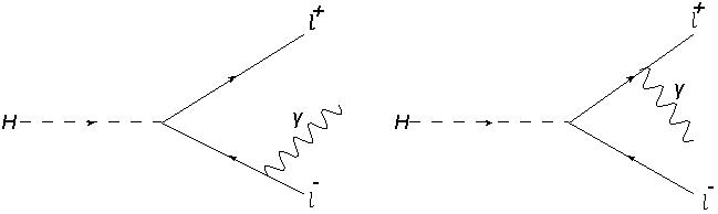
Figure 1: The tree level diagrams for $H\to\gamma\ell^{+}\ell^{-}$ decays, where $\ell$ corresponds to $\tau$.

2 Formulation of the Amplitude

The tree and the loop level Feynman diagrams for $H\to\gamma\tau^{+}\tau^{-}$ decays are shown in Figs. 1 and 2, respectively. The amplitudes for these diagrams can be expressed as AFB1

$$\mathcal{M}_{tree} = \mathcal{C}_{0}\bar{u}({p_{2}})\bigg{(}\frac{2p_{2}^{\nu}+\gamma^{\nu}\not{k}}{2p_{2}\dot{k}}-\frac{\not{k}\gamma^{\nu}+2p_{1}^{\nu}}{2p_{1}\dot{k}}\bigg{)}v({p_{1}})\epsilon_{\nu}^{*},$$

$$\mathcal{M}_{Loop} = \epsilon^{*\nu}(k_{\mu}q_{\nu}-g_{\mu\nu}(k.q))\bar{u}(p_{2})(\mathcal{C}_{1}\gamma^{\mu}+\mathcal{C}_{2}\gamma^{\mu}\gamma^{5})v(p_{1})$$ (2)

$$\quad+\epsilon_{\mu\nu\alpha\beta}\epsilon^{*\nu}k^{\alpha}q^{\beta}\bar{u}(p_{2})(\mathcal{C}_{3}\gamma^{\mu}+\mathcal{C}_{4}\gamma^{\mu}\gamma^{5})v(p_{1}),$$

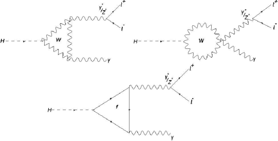
Figure 2: The $Z^{*}$ and $\gamma^{*}$ loop diagrams for $H\to\gamma\ell^{+}\ell^{-}$ decays, with $\ell$ corresponding to $\tau$ lepton.

with

$$\mathcal{C}_{0} = \frac{-2\pi\alpha m_{\tau}}{m_{W}sin\theta_{W}},$$

$$\mathcal{C}_{1} = -(\frac{1}{4}-sin^{2}\theta_{W})P_{Z}\Pi_{s\gamma Z}-\frac{1}{s}\Pi_{\gamma\gamma},\qquad\qquad\mathcal{C}_{2}=\frac{1}{4}P_{Z}\Pi_{s\gamma Z},$$

$$\mathcal{C}_{3} = -(\frac{1}{4}-sin^{2}\theta_{W})P_{Z}\Pi_{a\gamma Z}\qquad\qquad\qquad\qquad\mathcal{C}_{4}=\frac{1}{4}P_{Z}\Pi_{a\gamma Z}.$$ (3)

Here, $m_{\tau}$ denotes the mass of $\tau$ lepton, $p_{1}$, $p_{2}$, $k$ and $q$ are the momenta of $\tau^{-}$, $\tau^{+}$, $\gamma$ and the virtual particles $\gamma^{*}$ or $Z^{*}$, respectively. The fine structure constant is $\alpha$ while $\theta_{W}$ is the electroweak mixing angle. The definitions of the $P_{Z}$, $\Pi_{s\gamma Z}$, $\Pi_{\gamma\gamma}$ and $\Pi_{a\gamma Z}$ are given in ref. AFB1 , however, for the sake of completeness we have recollected them in the Appendix A.

Using these amplitudes, we have derived the expression of the the decay rate for the process $H\rightarrow\gamma\tau^{+}\tau^{-}$. Except a negative sign in the third term of the numerator of $\mathcal{B}$ defined below, our expression of the differential decay rate of $H\to\gamma\tau^{+}\tau^{-}$ decay is similar to the one given in ref. AFB1 and it can be expressed as follow:

$$\frac{d^{2}\Gamma}{dsdx}=\frac{(m_{H}^{2}-s)}{512\pi^{3}m_{H}^{3}}v\Delta,$$ (4)

with

$$\Delta = |\mathcal{C}_{0}|^{2}\mathcal{A}+2Re(\mathcal{C}_{0}C_{1}^{*})\mathcal{B}+2Re(\mathcal{C}_{0}\mathcal{C}_{4}^{*})\mathcal{C}$$ (5)

$$+(|\mathcal{C}_{1}|^{2}+|\mathcal{C}_{3}|^{2})\mathcal{D}+(|\mathcal{C}_{2}|^{2}+|\mathcal{C}_{4}|^{2})\mathcal{E}+2Re(\mathcal{C}_{1}\mathcal{C}_{4}^{*}+\mathcal{C}_{2}\mathcal{C}_{3}^{*})\mathcal{F},$$

and

$$\mathcal{A} = \frac{1}{(m_{H}^{2}-s)^{2}(1-v^{2}x^{2})^{2}}[m_{H}^{4}+s^{2}+32m_{\tau}^{4}-8m_{\tau}^{2}s-8m_{\tau}^{2}m_{H}^{2}-(m_{H}^{4}+s^{2}-8m_{\tau}^{2}s)v^{2}x^{2}],$$

$$\mathcal{B} = 8m_{\tau}\frac{m_{H}^{2}-s-sv^{2}(1-x^{2})}{1-v^{2}x^{2}},$$

$$\mathcal{C} = 8m_{\tau}\frac{(m_{H}^{2}-s)}{1-v^{2}x^{2}}vx,$$

$$\mathcal{D} = \frac{(m_{H}^{2}-s)^{2}}{2}(s+4m_{\tau}^{2}+s^{2}v^{2}x^{2}),$$

$$\mathcal{E} = \frac{(m_{H}^{2}-s)^{2}}{2}sv^{2}(1+x^{2}),$$

$$\mathcal{F} = (m_{H}^{2}-s)^{2}svx.$$ (6)

Here, $s$ is the square of momentum transfer i.e., $s=q^{2}$, $v=\sqrt{1-\frac{4m_{\tau}^{2}}{s}}$ and $x=cos\theta$ with $\theta$ is the angle between Higgs boson and a lepton in the rest frame of dileptons. The limits on the phase space parameters $s$ and $x$ are

$$4m_{\tau}^{2}\leq s\leq m_{H}^{2},\qquad-1\leq x\leq+1.$$ (7)

In Eq. (6), the term $\mathcal{A}$ represents the contribution from the tree diagrams where as $\mathcal{B}$ and $\mathcal{C}$ terms correspond to the interference between the tree and loop diagrams. The last three terms $\mathcal{D}$, $\mathcal{E}$ and $\mathcal{F}$ are originated purely from the loop diagrams.

3 Observables

It has already mentioned that the differential decay rate and the lepton forward-backward asymmetry were under debate in literature 6 ; 8 ; 9 ; 10 ; 11 ; AFB1 and the purpose of this study is to investigate the polarization asymmetries of the final state $\tau$ leptons in $H\to\gamma\tau^{+}\tau^{-}$ decay. To achieve this goal, let us introduce the orthogonal four vectors belonging to the polarization of $\tau^{-}$ and $\tau^{+}$, namely $S_{i}^{-}$ and $S_{i}^{+}$, respectively Polarization1 ; Polarization2 . These polarization vectors can be defined as follow:

$$S_{L}^{-\alpha}\equiv(0,\textbf{e}_{L}) = \left(0,\frac{\textbf{p}_{1}}{|\textbf{p}_{1}|}\right),$$

$$S_{N}^{-\alpha}\equiv(0,\textbf{e}_{N}) = \left(0,\frac{\textbf{k}\times\textbf{p}_{1}}{|\textbf{k}\times\textbf{p}_{1}|}\right),$$

$$S_{T}^{-\alpha}\equiv(0,\textbf{e}_{T}) = (0,\textbf{e}_{N}\times\textbf{e}_{L}),$$ (8)

where the subscripts $L$, $N$ and $T$ correspond to the longitudinal, normal and transverse polarizations, respectively. Also, $\textbf{p}_{1}$, $\textbf{p}_{2}$ and k are denoting the three momenta vectors of the final particles $\tau^{-}$, $\tau^{+}$ and $\gamma$, respectively, in the centre of mass frame of $\tau^{+}\tau^{-}$ system. It can be noticed that by replacing $\textbf{p}_{1}\to\textbf{p}_{2}$ one can obtain the unit vectors for the polarizations of $\tau^{+}$. The longitudinal unit vector $S_{L}$ are boosted by Lorentz transformations in the CM frame of $\tau^{+}\tau^{-}$:

$$S_{LCM}^{-\alpha} = \left(\frac{|\textbf{p}_{1}|}{m_{\tau}},\frac{E_{l}\textbf{p}_{1}}{m_{\tau}|\textbf{p}_{1}|}\right).$$ (9)

With these unit vectors, let us define the single lepton polarization asymmetry in the following way:

$$P_{i}^{(\pm)}(s) = \frac{\frac{d\Gamma}{ds}(\textbf{n}^{\pm}=\textbf{e}_{i}^{\pm})-\frac{d\Gamma}{ds}(\textbf{n}^{\pm}=-\textbf{e}_{i}^{\pm})}{\frac{d\Gamma}{ds}(\textbf{n}^{\pm}=\textbf{e}_{i}^{\pm})+\frac{d\Gamma}{ds}(\textbf{n}^{\pm}=-\textbf{e}_{i}^{\pm})},$$ (10)

where $\textbf{e}_{i}$ denotes the unit vector with subscript $i$ corresponds to longitudinal $(L)$, normal $(N)$ and transverse $(T)$ lepton polarizations index, and $\textbf{n}^{\pm}$ is the spin direction of $\tau^{\pm}$. The differential decay rate for the polarized lepton $\tau^{\pm}$ in $H\to\gamma\tau^{+}\tau^{-}$ decay along the spin direction $\textbf{n}^{\pm}$ is related to the unpolarized decay rate by the following relation:

$$\frac{d\Gamma(\textbf{n}^{\pm})}{ds}=\frac{1}{2}\left(\frac{d\Gamma}{ds}\right)\left[1+(P_{L}^{\pm}\textbf{e}_{L}^{\pm}+P_{N}^{\pm}\textbf{e}_{N}^{\pm}+P_{T}^{\pm}\textbf{e}_{T}^{\pm})\cdot\textbf{n}^{\pm}\right].$$ (11)

Finally, by using the definitions (10), the expressions for the longitudinal $(P_{L})$, normal $(P_{N})$, and transverse $(P_{T})$ lepton polarizations can be written as

$$P_{L}(s) = \frac{1}{\Delta}\bigg{[}\frac{4}{3}sv\left(m_{H}^{2}-s\right)^{2}[2\mathcal{R}e(\mathcal{C}_{1}\mathcal{C}_{2}^{*})+2\mathcal{R}e(\mathcal{C}_{3}\mathcal{C}_{4}^{*})]-\frac{4m_{\tau}\left(m_{H}^{2}-s\right)}{sv^{2}}\{\tanh^{-1}(v)\left(4m_{\tau}^{2}-sv^{2}+s\right)$$

$$+s^{2}v\left(v^{2}-1\right)2\mathcal{R}e(\mathcal{C}_{0}\mathcal{C}_{3}^{*})-\{2\left(sv^{2}+s\right)\tanh^{-1}(v)+sv(v^{2}-1)\}2\mathcal{R}e(\mathcal{C}_{0}\mathcal{C}_{2}^{*})\}\bigg{]},$$

$$P_{N}(s) = \frac{1}{\Delta}\bigg{[}-2\{\frac{4\pi m_{\tau}^{2}m_{H}^{2}\left(2v^{2}+\sqrt{1-v^{2}}+1\right)}{\sqrt{s}v^{2}\sqrt{1-v^{2}}}-\frac{\pi\sqrt{s}\left(\sqrt{1-v^{2}}+1\right)\left(4m_{\tau}^{2}+m_{H}^{2}-s\right)}{v^{2}}+\frac{2\sqrt{s}\left(m_{H}^{2}-2s\right)}{v}$$ (13)

$$+\frac{4m_{\tau}^{2}\sqrt{s}\left(2\sqrt{1-v^{2}}+\pi v\right)}{v\sqrt{1-v^{2}}}-\sqrt{s}\left(8m_{\tau}^{2}+(2+\pi)m_{H}^{2}-(\pi-4)s\right)\}\mathcal{R}e(\mathcal{C}_{0}\mathcal{C}_{2}^{*})$$

$$+\{\frac{2\pi}{s^{3/2}v^{2}\sqrt{1-v^{2}}}\left(4m_{\tau}^{2}\left(m_{H}^{2}+s\right)+s\left(m_{H}^{2}-3s\right)\right)\left(4m_{\tau}^{2}-s\left(v^{2}+2\sqrt{1-v^{2}}-1\right)\right)\}\mathcal{R}e(\mathcal{C}_{0}\mathcal{C}_{3}^{*})$$

$$+\pi m_{\tau}\sqrt{s}\left(m_{H}^{2}-s\right)^{2}[2\mathcal{R}e(\mathcal{C}_{1}\mathcal{C}_{3}^{*})]\bigg{]},$$

$$P_{T}(s) = \frac{1}{\Delta}\bigg{[}\pi v\sqrt{s}\left(\text{m}_{H}^{2}-s\right)\left\{2\big{[}2\mathcal{I}m(\mathcal{C}_{1}^{*}\mathcal{C}_{0})+2\mathcal{I}m(\mathcal{C}_{4}^{*}\mathcal{C}_{0})\big{]}-m_{\tau}\left(\text{m}_{H}^{2}-s\right)\big{[}2\mathcal{I}m(\mathcal{C}_{4}^{\ast}\mathcal{C}_{1})+2\mathcal{I}m(\mathcal{C}_{2}^{\ast}\mathcal{C}_{3})\big{]}\right\}\bigg{]},$$

where $\mathcal{C}_{0},\ldots,\mathcal{C}_{4}$ are given in Eq. (3) and the $\Delta$ used in the above equations is defined in Eq. (5).

To calculate the double-lepton-polarization asymmetries, we consider the polarizations of both $\tau^{-}$ and $\tau^{+}$ simultaneously and introduce the following spin projection operators for the $\tau^{-}$ and $\tau^{+}$,

$$\Lambda_{1} = \frac{1}{2}\left(1+\gamma_{5}\not{S}_{i}^{-}\right),$$

$$\Lambda_{2} = \frac{1}{2}\left(1+\gamma_{5}\not{S}_{i}^{+}\right),$$ (15)

where $i=L,T\,\$and $N$ again designate the longitudinal, transverse and normal lepton polarizations index, respectively. In the rest frame of the $\tau^{-}\tau^{+}$ one can define the following set of orthogonal vectors $S^{\alpha}$:

$$S_{L}^{-\alpha} = (0,\textbf{e}_{L}^{-})=\left(0,\frac{\textbf{p}_{1}}{\left|\textbf{p}_{1}\right|}\right),$$

$$S_{N}^{-\alpha} = (0,\textbf{e}_{N}^{-})=\left(0,\frac{\textbf{k}\times\textbf{p}_{1}}{\left|\textbf{k}\times\textbf{p}_{1}\right|}\right),$$

$$S_{T}^{-\alpha} = (0,\textbf{e}_{T}^{-})=\left(0,\textbf{e}_{N}^{-}\times\textbf{e}_{L}^{-}\right),$$ (16)

$$S_{L}^{+\alpha} = (0,\textbf{e}_{L}^{+})=\left(0,\frac{\textbf{p}_{2}}{\left|\textbf{p}_{2}\right|}\right),$$

$$S_{N}^{+\alpha} = (0,\textbf{e}_{N}^{+})=\left(0,\frac{\textbf{k}\times\textbf{p}_{2}}{\left|\textbf{k}\times\textbf{p}_{2}\right|}\right),$$

$$S_{T}^{+\alpha} = (0,\textbf{e}_{T}^{+})=\left(0,\textbf{e}_{N}^{+}\times\textbf{e}_{L}^{+}\right).$$

Just like the single lepton polarizations, through Lorentz transformations we can boost the longitudinal component in the CM frame of $\tau^{-}\tau^{+}$ as

$$\left(S_{L}^{-\alpha}\right)_{CM} = \left(\frac{|\textbf{p}_{1}|}{m_{l}},\frac{E\textbf{p}_{1}}{m_{l}\left|\textbf{p}_{-}\right|}\right),$$

$$\left(S_{L}^{+\alpha}\right)_{CM} = \left(\frac{|\textbf{p}_{2}|}{m_{l}},-\frac{E\textbf{p}_{2}}{m_{l}\left|\textbf{p}_{+}\right|}\right).$$ (17)

The normal and transverse components remain the same under Lorentz boost. We now define the double lepton polarization asymmetries as

$$P_{ij}(s)=\frac{\left(\frac{d\Gamma}{ds}\left(\textbf{S}_{i}^{-},\textbf{S}_{j}^{+}\right)-\frac{d\Gamma}{ds}\left(-\textbf{S}_{i}^{-},\textbf{S}_{j}^{+}\right)\right)-\left(\frac{d\Gamma}{ds}\left(\textbf{S}_{i}^{-},-\textbf{S}_{j}^{+}\right)-\frac{d\Gamma}{ds}\left(-\textbf{S}_{i}^{-},-\textbf{S}_{j}^{+}\right)\right)}{\left(\frac{d\Gamma}{ds}\left(\textbf{S}_{i}^{-},\textbf{S}_{j}^{+}\right)-\frac{d\Gamma}{ds}\left(-\textbf{S}_{i}^{-},\textbf{S}_{j}^{+}\right)\right)+\left(\frac{d\Gamma}{ds}\left(\textbf{S}_{i}^{-},-\textbf{S}_{j}^{+}\right)-\frac{d\Gamma}{ds}\left(-\textbf{S}_{i}^{-},-\textbf{S}_{j}^{+}\right)\right)},$$ (18)

where the subscripts $i$ and $j$ correspond to the $\tau^{-}$ and $\tau^{+}$ polarizations indices, respectively. Using these definitions the various double lepton polarization asymmetries as a function of $s$ can be written as

$$P_{LL}(s) = \frac{1}{\Delta}\bigg{[}\frac{32}{s^{2}v^{3}\left(m_{H}^{2}-s\right)^{2}}\{\tanh^{-1}(v)(-64m_{\tau}^{6}s+8m_{\tau}^{4}(m_{H}^{4}+7s^{2})-4m_{\tau}^{2}s(m_{H}^{4}-m_{H}^{2}s+5s^{2})$$

$$+s^{2}(m_{H}^{4}+2m_{H}^{2}s(v^{2}-1)+s^{2}(3-2v^{2})))-sv(16m_{\tau}^{4}s-2m_{\tau}^{2}(m_{H}^{4}+3s^{2})$$

$$+s(m_{H}^{4}-m_{H}^{2}s+s^{2}))\}\left|\mathcal{C}_{0}\right|^{2}+\frac{(m_{H}^{2}-s)^{2}}{3m_{\tau}^{2}}\{(8m_{\tau}^{4}+s^{2}(v^{2}-1))(\left|\mathcal{C}_{1}\right|^{2}+\left|\mathcal{C}_{3}\right|^{2})$$

$$+s^{2}v^{2}(v^{2}-1)(\left|\mathcal{C}_{4}\right|^{2}+\left|\mathcal{C}_{2}\right|^{2})\}-\frac{8}{m_{\tau}sv^{3}}\{m_{\tau}^{2}sv(2sv^{2}-2(m_{H}^{2}-s)-v^{3}(m_{H}^{2}-s))$$

$$+\tanh^{-1}(v)(64m_{\tau}^{6}-16m_{\tau}^{4}s-8m_{\tau}^{2}s^{2}-s^{2}(v^{2}-1)(2s+v^{3}(m_{H}^{2}-s)))\}(2\mathcal{R}_{e}(\mathcal{C}_{0}\mathcal{C}_{1}^{*}))$$

$$+\frac{2}{m_{\tau}s}\{(m_{H}^{2}-s)(s(4m_{\tau}^{2}+sv^{5/2}-sv^{3})-\tanh^{-1}(v)((4m_{\tau}^{2}+s)^{2}-s^{2}v^{3}))(2\mathcal{R}_{e}(\mathcal{C}_{0}\mathcal{C}_{4}^{*}))\}\bigg{]},$$

$$P_{NN}(s) = \frac{1}{\Delta}\bigg{[}\frac{32}{v(m_{H}^{2}-s)^{2}}\{(2(m_{H}^{2}-s)(2m_{\tau}^{2}-s)+s^{2}v^{2}(v^{2}+1))\tanh^{-1}(v)+sv(m_{H}^{2}+s(v^{2}-1)\}\left|\mathcal{C}_{0}\right|^{2}$$

$$+\frac{2}{3}sv^{2}(m_{H}^{2}-s)^{2}\{(\left|\mathcal{C}_{1}\right|^{2}+\left|\mathcal{C}_{3}\right|^{2})-(\left|\mathcal{C}_{4}\right|^{2}+\left|\mathcal{C}_{2}\right|^{2})\}-\frac{8m_{\tau}}{v}\{8m_{\tau}^{2}\tanh^{-1}(v)+s(\pi-2v)\}(2\mathcal{R}_{e}(\mathcal{C}_{0}\mathcal{C}_{1}^{*}))\bigg{]},$$

$$P_{TT}(s) = \frac{1}{\Delta}\bigg{[}-\frac{32}{s^{2}v^{3}(m_{H}^{2}-s)^{2}}(16m_{\tau}^{4}s+2m_{\tau}^{2}(m_{H}^{4}-4m_{H}^{2}s-s^{2})+m_{H}^{2}s^{2})(sv-s(v^{2}+1)\tanh^{-1}(v))\left|\mathcal{C}_{0}\right|^{2}$$ (21)

$$+\frac{16m}{sv^{3}}(2m_{\tau}^{2}\tanh^{-1}(v)(-m_{H}^{2}+2sv^{2}+s)-s^{2}v^{3})(2\mathcal{R}e(\mathcal{C}_{0}\mathcal{C}_{1}^{*}))$$

$$+\frac{2}{3}s(m_{H}^{2}-s)^{2}\big{(}(2-v^{2})(\left|\mathcal{C}_{1}\right|^{2}+\left|\mathcal{C}_{3}\right|^{2})-v^{2}(\left|\mathcal{C}_{4}\right|^{2}+\left|\mathcal{C}_{2}\right|^{2})\big{)}\bigg{]},$$

$$P_{LN}(s) = \frac{1}{\Delta}\bigg{[}\frac{\pi}{2v^{2}}\sqrt{s}(m_{H}^{2}-s)\{-4\sqrt{1-v^{2}}(\frac{2m_{\tau}^{2}}{s}+v^{2})-\frac{8m_{\tau}^{2}}{s}+2v^{2}+2\}((2\mathcal{I}m(\mathcal{C}_{0}\mathcal{C}_{2}^{\ast}))$$ (22)

$$+ 2\pi\sqrt{s}(\sqrt{1-v^{2}}-1)(m_{H}^{2}-s)(2\mathcal{I}m(\mathcal{C}_{0}\mathcal{C}_{3}^{*}))\bigg{]}=-P_{NL}(s),$$

$$P_{LT}(s) = \frac{1}{\Delta}\bigg{[}-\frac{16\pi m_{\tau}}{\sqrt{s}\sqrt{\frac{1}{v^{2}}-1}}\left|\mathcal{C}_{0}\right|^{2}$$ (23)

$$+\frac{1}{2}\pi m_{\tau}\sqrt{s}v\left(m_{H}^{2}-s\right)^{2}(2\mathcal{R}e(\mathcal{C}_{1}\mathcal{C}_{4}^{*})+2\mathcal{R}e(\mathcal{C}_{2}\mathcal{C}_{3}^{*}))-\frac{2\pi\sqrt{s}\left(\sqrt{1-v^{2}}-1\right)\left(m_{H}^{2}-s\right)}{v}(2\mathcal{R}e(\mathcal{C}_{0}\mathcal{C}_{1}^{*}))$$

$$+\frac{\left(m_{H}^{2}-s\right)}{2s^{3/2}v^{2}}\{\pi\left\{-16m_{\tau}^{4}+8m_{\tau}^{2}s+s^{2}\left(v^{4}+3\right)\right\}-8\pi m_{\tau}s\sqrt{2m_{\tau}^{2}+sv^{2}}\}(2\mathcal{R}e(\mathcal{C}_{0}\mathcal{C}_{4}^{*}))\bigg{]}\-P_{TL},$$

$$P_{NT}(s) = \frac{8m_{\tau}}{\Delta v^{2}}\bigg{[}\left(m_{H}^{2}-s\right)\left(\left(v^{2}-1\right)\tanh^{-1}(v)+v\right)(2\mathcal{I}m(\mathcal{C}_{0}\mathcal{C}_{3}^{\ast}))+\left(4m_{\tau}^{2}\tanh^{-1}(v)-sv\right)(2\mathcal{I}m(\mathcal{C}_{0}\mathcal{C}_{2}^{\ast}))\bigg{]}$$ (24)

$$= -P_{TN},$$

with $\mathcal{C}_{0},\ldots,\mathcal{C}_{4}$ and $\Delta$ used in above equations are defined in Eq. (3) and Eq. (5), respectively.

Table 1: Default values of input parameters used in the calculations

$m_{H}=125$ GeV, $m_{t}=172$ GeV, $m_{\mu}=0.106$ GeV,

$m_{e}=0.51\times 10^{-3}$ GeV, $m_{\tau}=1.77$ GeV, $\alpha(M_{Z})^{-1}=128$,

$m_{Z}=91.18$ GeV, $\Gamma_{Z}=2.48$ GeV.

4 Numerical Analysis

In the previous section we have presented the expressions of the single and double lepton polarization asymmetries in the SM for $H\to\gamma\tau^{+}\tau^{-}$ decay by considering both tree and loop diagrams. To proceed with the numerical analysis of these physical observables, the numerical values of different input parameters in the SM are listed in Table 1.

4.1 Single Lepton Polarization Asymmetries

Similar to the case of leptons forward-backward asymmetries $A_{FB}$ calculated in ref. AFB1 , one can see from Eqs. (LABEL:pl1, 13, LABEL:pl3) that the single lepton polarization asymmetries are not separately dependent on the tree level diagrams. However, they depend on the interference of the contributions from different loop diagrams (c.f. Figure 2) as well as on the interference of tree and loop diagrams. Moreover, for the longitudinal polarization asymmetry $P_{L}$ the contributions generated from the interference between tree and loop diagrams $\mathcal{C}_{0}\mathcal{C}_{3}^{*}$ and $\mathcal{C}_{0}\mathcal{C}_{2}^{*}$ are $m_{\tau}$ suppressed.

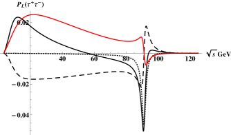
Figure 3: The longitudinal lepton polarization asymmetry $P_{L}(s)$ in $H\to\gamma\tau^{+}\tau^{-}$ as a function of the momentum transfer $\sqrt{s}$. The solid line correspond to the total contribution, the dashed line correspond to the contribution through the interference between the tree diagram and $Z^{\ast}$ pole diagrams and the dotted line corresponds to the contribution from the $Z^{\ast}-Z^{\ast}$ interference while the red line corresponds to the contribution from the $\gamma^{\ast}-Z^{\ast}$ interference.

Figure 4: The Normal lepton polarization asymmetry $P_{N}(s)$ in $H\to\gamma\tau^{+}\tau^{-}$ as a function of the momentum transfer $\sqrt{s}$. The solid line corresponds to the $P_{N}$ and the dashed line is for $P_{T}$.

$s_{min}-s_{max}(\text{GeV}^{2})$	$10^{2}-30^{2}$	$30^{2}-50^{2}$	$50^{2}-70^{2}$	$70^{2}-90^{2}$	$90^{2}-110^{2}$	full Phase space
$H\to\gamma\tau^{+}\tau^{-}$	3.3%	4.8%	5.4%	7.9%	-1.3%	0.02%

Table 2: The average Normal polarization asymmetries $\langle P_{N}\rangle$ for some cuts on $s$ in $H\to\gamma\tau^{+}\tau^{-}$ decays .

The longitudinal lepton polarization $P_{L}$ as a function of $\sqrt{s}$ in $H\to\gamma\tau^{+}\tau^{-}$ is drawn in Fig. 3. It is expected from Eq. (LABEL:pl1) that the major contribution is coming through the interference of different loop diagrams. If we recall Eq. (3) for the definitions of $\mathcal{C}_{1}-\mathcal{C}_{4}$ then there are two types of contributions, namely, $\gamma^{*}-Z^{*}$ interference (referred as the overlap between the $\gamma^{*}$ pole amplitude and the $Z^{*}$ pole amplitude) and the second one is $Z^{*}-Z^{*}$ interference (i.e. the interference among the different amplitudes of $Z^{*}$ pole diagrams). Similar to the $A_{FB}$ AFB1 the longitudinal polarization asymmetry also has zero crossing because of the change of sign of $\gamma^{*}-Z^{*}$ interference at $s=m_{Z}^{2}$ which is due to the sign change of the real part of $P_{Z}$ and it is evident from Fig. 3. It can also be seen from Figure 3 that throughout the allowed kinematical region the value of $P_{L}$ in $H\to\gamma\tau^{+}\tau^{-}$ is of the order of $10^{-2}$ and to measure such a small number at the current colliders is not an easy task.

In contrast to the longitudinal lepton polarization asymmetry $(P_{L})$ and the leptons forward-backward asymmetry $(A_{FB})$, the contributions from the loop diagrams (c.f. contributions from the $Z^{*}-Z^{*}$ and $\gamma^{*}-Z^{*}$ interference ) are $m_{\tau}$ suppressed in the normal lepton polarization asymmetry $(P_{N})$ and hence can be safely ignored. The normal lepton polarization ($P_{N}$), where the contribution is coming from the interference between the tree and $Z^{*}$ pole diagrams is displayed with solid line in Figure 4.

Just like the leptons forward-backward asymmetry $(A_{FB})$ calculated in ref. AFB1 , the magnitude of transverse lepton polarization asymmetry $(P_{T})$ is very small in almost all the kinematical region and the dahsed line in Figure 4 demonstrate this fact. By looking at the Eq. (LABEL:pl3) it is even more evident that it is proportional to the imaginary part of the contributions from different interference diagrams which are too small, hence we ignored its detailed analysis over here.

Furthermore, we have also calculated the average value of normal polarization asymmetry $(P_{N})$ in different bins of $s$ and listed it in Tables 2 for $H\to\gamma\tau^{+}\tau^{-}$. It is clear from the Table 2 that by scanning full phase space altogether this asymmetry might not be measurable quantities at LHC, but by making an analysis in different bins of $s$ the average value of normal lepton polarization asymmetry may be measurable at the LHC.

4.2 Double Lepton Polarization Asymmetries

Now we discuss the double lepton polarization asymmetries $P_{ij}$, where the indices $i,j$ can be $L$, $T$ and $N$. In Section 3, we have derived the expressions of different double lepton polarization asymmetries (c.f. Eqs. (LABEL:pll1-21)), where one can immediately notice that in contrast to the above discussed single lepton polarization asymmetries and the forward-backward asymmetries, discussed in length in ref. AFB1 , some of the $P_{ij}$’s are explicit functions of the tree diagrams in addition to their interference with loop diagrams.

$s_{min}-s_{max}(\text{GeV}^{2})$	$10^{2}-30^{2}$	$30^{2}-50^{2}$	$50^{2}-70^{2}$	$70^{2}-90^{2}$	$90^{2}-110^{2}$	full Phase space
$H\to\gamma\tau^{+}\tau^{-}$	86.7%	80.8%	84.7%	84.6%	93.8%	99.6%

Table 3: The average polarization asymmetries $\langle P_{LL}\rangle$ for some cuts on $s$ in $H\to\gamma\tau^{+}\tau^{-}$ decays .

The double longitudinal lepton polarization asymmetry ($P_{LL}$) in $H\to\gamma\tau^{+}\tau^{-}$ as a function of $\sqrt{s}$ is drawn in Fig. 5. Fig. 5 shows that in the $H\to\gamma\tau^{+}\tau^{-}$ decay the major contribution is coming from the tree diagram which is denoted by the red line in this figure. The average value of $P_{LL}$ in various bins of $s$ is given in Table 3 where we can see that this asymmetry has a significantly large value in the whole phase space range. From experimental point of view, it has already been mentioned that the reconstruction of the polarization is possible only if the particle is unstable and due to the decay of $\tau$ lepton to a final state charged hadron its spin direction is inferred from the decay products distribution Sug1 ; Sug2 at the LHC. Therefore, the scanning of double longitudinal lepton polarization asymmetry at the LHC will help us to dig out some intrinsic properties of the Higgs particle and its dynamics.

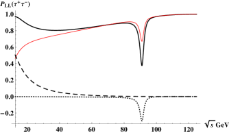
Figure 5: $P_{LL}(s)$ in $H\to\gamma\tau^{+}\tau^{-}$ as a function of the momentum transfer $\sqrt{s}$. The solid line correspond to the total contribution, the red line correspond to the contribution coming from only tree diagrams and the dotted line corresponds to the contribution from the $Z^{\ast}-Z^{\ast}$ interference while the dashed line corresponds to the contribution from the interference of tree diagrams and $\gamma^{*}$ diagrams. The other contributions are too small to be shown here.

$s_{min}-s_{max}(\text{GeV}^{2})$	$10^{2}-30^{2}$	$30^{2}-50^{2}$	$50^{2}-70^{2}$	$70^{2}-90^{2}$	$90^{2}-110^{2}$	full Phase space
$H\to\gamma\tau^{+}\tau^{-}$	-7%	18%	41.7%	64.6%	88.7%	99%

Table 4: The average polarization asymmetries $\langle P_{TT}\rangle$ for some cuts on $s$ in $H\to\gamma\tau^{+}\tau^{-}$ decay.

Fig. 6 display the behavior of $P_{TT}$ as a function of $\sqrt{s}$ for $H\to\gamma\tau^{+}\tau^{-}$ decay where the major contribution is coming from the tree diagram and it is denoted by the red line in Fig. 6. In Fig. 6 one can see that in the region $90$GeV$\leq\sqrt{s}\leq\sqrt{s}_{max}$ the major contribution is coming only from the tree diagrams and it can be seen that the average value of $\langle P_{TT}\rangle$ enhanced upto $88\%$ in this region (c.f. Table 5) which is in a measurable ball park of the LHC.

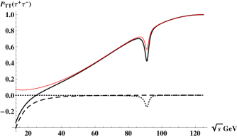
Figure 6: $P_{TT}(s)$ in $H\to\gamma\tau^{+}\tau^{-}$ as a function of the momentum transfer $\sqrt{s}$. The legends are same as in Fig. 5.

$s_{min}-s_{max}(\text{GeV}^{2})$	$10^{2}-30^{2}$	$30^{2}-50^{2}$	$50^{2}-70^{2}$	$70^{2}-90^{2}$	$90^{2}-110^{2}$	full Phase space
$H\to\gamma\tau^{+}\tau^{-}$	-6.2%	-20.2%	-42.6%	-68.7%	-90.8%	-99.1%

Table 5: The average polarization asymmetries $\langle P_{NN}\rangle$ for some cuts on $s$ in $H\to\gamma\tau^{+}\tau^{-}$ decays.

Similarly, $P_{NN}$ in $H\to\gamma\tau^{+}\tau^{-}$ as a function of $\sqrt{s}$ is drawn in Fig. 7. From Fig. 7 we can notice that in $H\to\gamma\tau^{+}\tau^{-}$, the terms contributing to $P_{NN}$ are coming from the tree diagrams. In order to make the analysis more clear the values of average $P_{NN}$ in various bins of $s$ are given in the Table 6. We can see that in the region $50$GeV$<\sqrt{s}<110$GeV, the average values of double normal lepton polarization asymmetry enhanced up to $91\%$ for $H\to\gamma\tau^{+}\tau^{-}$ decay. Therefore, it will be interesting to scan the $P_{NN}$ in different bins of $s$ to clear the smog from the Higgs decays.

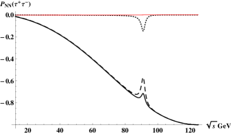
Figure 7: $P_{NN}(s)$ in $H\to\gamma\tau^{+}\tau^{-}$ as a function of the momentum transfer $\sqrt{s}$. The solid line correspond to the total contribution, the dotted line corresponds the $Z^{*}-Z^{*}$ interference contribution and the red line corresponds to the contribution from $Z^{*}-\gamma^{*}$ interference while the dashed line corresponds to the contribution from the tree diagrams. The other contributions are too small to be shown here.

$s_{min}-s_{max}(\text{GeV}^{2})$	$10^{2}-30^{2}$	$30^{2}-50^{2}$	$50^{2}-70^{2}$	$70^{2}-90^{2}$	$90^{2}-110^{2}$	full Phase space
$H\to\gamma\tau^{+}\tau^{-}$	-43.6%	-28.1%	-15.7%	-6.5%	-1.7%	-4.2%

Table 6: The average polarization asymmetries $\langle P_{LT}\rangle$ for some cuts on $s$ in $H\to\gamma\tau^{+}\tau^{-}$ decay.

Figure 8: $P_{LT}(s)$ in $H\to\gamma\tau^{+}\tau^{-}$ as a function of the momentum transfer $\sqrt{s}$. The solid line correspond to the total contribution, the red line corresponds to the contribution coming from the interference between tree diagrams and $Z^{*}$ pole diagrams and the dotted line corresponds to the contribution from the interference between tree diagrams and the $\gamma^{*}$ diagrams while the dashed line corresponds to the contribution from the tree diagrams only. The other contributions are negligible.

In $H\to\gamma\tau^{+}\tau^{-}$ the $P_{LT}$ as a function of $\sqrt{s}$ is displayed in Fig. 8, where one can see that the major contribution is through the tree diagrams, represented by the dashed line in Fig. 8. The contributions from the other diagrams come out to be negligible to show in the graphs. Finally, the average values of $P_{LT}$ is listed in Table 7 in various bins of the $s$. Remarkably, in contrast to the lepton forward-backward asymmetry $A_{FB}$ AFB1 , like other polarization asymmetries the value of $P_{LT}$ for $H\to\gamma\tau^{+}\tau^{-}$ is significantly large in different regions of $s$, and we hope that these can be measured at the LHC.

Figure 9: $P_{LN}(s)$ and $P_{TN}$ as a function of the momentum transfer $\sqrt{s}$ in $H\to\gamma\tau^{+}\tau^{-}$ decay. The solid line corresponds to the $P_{LN}$ and the dashed line refers to the $P_{TN}$.

In Fig. 9 we have plotted $P_{LN}$ and $P_{TN}$ as a function of $\sqrt{s}$ in $H\to\gamma\tau^{+}\tau^{-}$ decay, where the solid and dashed lines correspond to the $P_{LN}$ and $P_{TN}$, respectively. From Eqs. (22) and (24), it is clear that these two asymmetries are proportional to the imaginary part of the contributions arising from different diagrams, encoded in $\mathcal{C}^{\prime}s$ and hence their value is expected to be small and it is clear from Fig. 9. In case of $P_{LN}$, the contribution is coming from the interference between tree and $Z^{*}$ pole diagrams and for $P_{TN}$ it is coming from the interference between tree and $\gamma^{*}$ diagrams, while the other contributions are small enough to plot at the present scale.

5 Conclusion

In this work we have calculated the single and double lepton polarization asymmetries in $H\to\gamma\tau^{+}\tau^{-}$ decay. To calculate these asymmetries we consider both the tree and loop level diagrams. First, we have derived the expressions of these asymmetries and then explicitly evaluated the SM contributions of these diagrams to $P_{i}$ and $P_{ij}$, where $i,j$ can be $L$, $N$ or $T$. We have found that both type of diagrams are significant in the calculation of the SM values of the above mentioned asymmetries. The analysis shows that the separate contribution of the tree level diagrams for the single lepton polarization asymmetries is absent, just like in the forward-backward asymmetries $A_{FB}$ AFB1 , which however is present in the the double lepton polarization asymmetries. Particularly, in $P_{LL}$ and $P_{TT}$ for $H\to\gamma\tau^{+}\tau^{-}$ the contributions from the tree level diagrams are the dominant one.

As one of the major motivation of this study is to see either the magnitude of the asymmetries other than the forward-backward asymmetries is large enough to be measured or not. Regarding this, interestingly, the numerical calculations performed here show that most of the single and double lepton polarization asymmetries comes out to be an order of magnitude larger than the forward-backward asymmetries $A_{FB}$ calculated in ref.AFB1 .

To highlight, by analyzing the different single and double lepton polarization asymmetries in $H\to\gamma\tau^{+}\tau^{-}$ decay, we found that the average values of these asymmetries in some kinematical region are sufficiently large (c.f. Tables 4-7) than the forward-backward asymmetries $A_{FB}$ AFB1 which can be measured at the current colliders. To keep an eye on the features of the $A_{FB}$, $P_{i}$ and $P_{ij}$ we would comparatively assume that the later polarization asymmetries are good observable in $H\to\gamma\tau^{+}\tau^{-}$. Therefore, the measurement of different single and double lepton polarization asymmetries for $H\to\gamma\tau^{+}\tau^{-}$ decay will definitely help out to clear some smog from the intrinsic properties of Higgs boson and its dynamics.

Appendix A Appendix

The function $P_{Z}$ is defined as

$$P_{Z}=\frac{1}{sin\theta_{W}cos\theta_{W}}\frac{1}{s-m_{Z}^{2}+im_{Z}\Gamma_{Z}},$$ (25)

where $s=q^{2}=(p_{1}+p_{2})^{2}$ is square of momentum transfer to the lepton pair, $\theta_{W}$ is the weak mixing angle and $\Gamma_{Z}$ is the decay width of $Z$ boson. The functions $\Pi_{\alpha\gamma Z}$, $\Pi_{s\gamma Z}$ and $\Pi_{\gamma\gamma}$ are induced from the $Z^{*}$ and $\gamma^{*}$ pole diagrams given in Fig. 2 and these can be summarized as follows:

$$\Pi_{a\gamma Z}=\frac{\alpha^{2}}{m_{W}sin\theta_{W}}\frac{N_{c}Q_{f}T_{f}}{sin{\theta_{W}}cos\theta_{W}}A_{f_{2}}(\tau_{f},\lambda_{f}),$$ (26)

$$\Pi_{s\gamma Z}=\frac{\alpha^{2}}{m_{W}sin\theta_{W}}\bigg{[}-cot\theta_{W}A_{W}(\tau_{W},\lambda_{W})$$

$$-2N_{c}Q_{f}\frac{T_{f}-2Q_{f}sin^{2}\theta_{W}}{sin\theta_{W}cos\theta_{W}}A_{f_{1}}(\tau_{f},\lambda_{f})\bigg{]},$$ (27)

$$\Pi_{\gamma\gamma}=\frac{\alpha^{2}}{m_{W}sin\theta_{W}}\bigg{[}-A_{W}(\tau_{W},\lambda_{W})-4N_{c}Q_{f}^{2}A_{f_{1}(\tau_{f},\lambda_{f})}\bigg{]}.$$ (28)

Here, the functions $A_{W}$, $A_{f_{1}}$ and $A_{f_{2}}$ denote the contributions from the $W$ boson and fermion loops, with $\tau=\frac{4m^{2}_{i}}{m^{2}_{H}}$, $\lambda_{i}=\frac{4m^{2}_{i}}{q^{2}}(i=f,W)$, $m_{f}$ is the fermion mass, $N_{c}$ the color multiplication, $Q_{f}$ is fermion charge, $\tau_{f}$ is the third component of weak isospin of fermion $f$ inside the loop. Expressions of these loop functions can be summarized as

$$A_{f_{1}}(\tau,\lambda)=I_{1}(\tau,\lambda)-I_{2}(\tau,\lambda),$$ (29)

$$A_{f_{2}}(\tau,\lambda)=\frac{\tau\lambda}{\lambda-\tau}[2g(\tau)-2g(\lambda)+f(\tau)-f(\lambda)],$$ (30)

$$A_{W}(\tau,\lambda)=\bigg{[}\left(1+\frac{2}{\tau}\right)\left(\frac{4}{\lambda}-1\right)-\left(5+\frac{2}{\tau}\right)\bigg{]}I_{1}(\tau,\lambda)+16\left(1-\frac{1}{\lambda}\right)I_{2}(\tau,\lambda)$$ (31)

with

$$I_{1}(\tau,\lambda)=\frac{\tau\lambda}{2(\tau-\lambda)}+\frac{\tau^{2}\lambda^{2}}{2(\tau-\lambda)^{2}}[f(\tau)-f(\lambda)]+\frac{\tau^{2}\lambda}{(\tau-\lambda)^{2}}[g(\tau)-g(\lambda)],$$ (32)

$$I_{2}(\tau,\lambda)=-\frac{\tau\lambda}{2(\tau-\lambda)}[f(\tau)-f(\lambda)],$$ (33)

and

$$f(\tau) = \begin{cases}arcsin^{2}(\tau^{(-\frac{1}{2})})&\text{for }\tau\geq 1\\ -\frac{1}{4}\bigg{[}\ln\frac{1+\sqrt{1-\tau}}{1-\sqrt{1-\tau}}-i\pi\bigg{]}^{2}{}&\text{for }\tau<1,\end{cases}$$ (34)

$$g(\tau) = \begin{cases}\sqrt{\tau-1}arcsin(\tau^{(-\frac{1}{2})})&\text{for }\tau\geq 1\\ \frac{\sqrt{1-\tau}}{2}\bigg{[}\ln\frac{1+\sqrt{1-\tau}}{1-\sqrt{1-\tau}}-i\pi\bigg{]}&\text{for }\tau<1.\end{cases}$$ (35)

References

- (1) G. Aad et al. [ATLAS Collaboration], Observation of a new particle in the search for the Standard Model Higgs boson with the ATLAS detector at the LHC, Phys. Lett. B716 (2012) 1; [arXiv:1207.7214[hep-ex]].
- (2) S. Chatrchyan et al. [CMS Collaboration], Observation of a new boson at a mass of 125 GeV with the CMS experiment at the LHC, Phys. Lett. B716 (2012) 30; [arXiv:1207.7235[hep-ex]]; Observation of a new boson with mass near 125 GeV in PP collisions at ps=7 TeV and 8 TeV, arXiv:1303.4571[hep-ex].
- (3) F. J. Petriello, Kaluza-Klein effects on Higgs physics in universal extra dimensions, JHEP 0205, 003 (2002) [arXiv: hep-ph/0204067].
- (4) T. Han, H. E. Logan, B. McElrath and L. -T. Wang, Loop induced decays of the little Higgs: Phys. Lett. B 563, 191 (2003) [Erratum-ibid. B 603, 257 (2004)] [arXiv: hep-ph/0302188].
- (5) G. Cacciapaglia, A. Deandrea and J. Llodra-Perez, beyond the Standard Model, JHEP 0906, 054 (2009) [arXiv:0901.0927 [hep-ph]].
- (6) J. Cao, Z. Heng, T. Liu and J. M. Yang, Di-photon Higgs signal at the LHC: A Comparative study for different supersymmetric models, Phys. Lett. B 703, 462 (2011) [arXiv:1103.0631 [hep-ph]].
- (7) S. Heinemeyer, O. Stal and G. Weiglein, Interpreting the LHC Higgs Search Results in the MSSM, Phys. Lett. B 710, 201 (2012) [arXiv:1112.3026 [hep-ph]].
- (8) P. M. Ferreira, R. Santos, M. Sher and J. P. Silva, Implications of the LHC two-photon signal for two-Higgs-doublet models, Phys. Rev. D 85, 077703 (2012) [arXiv:1112.3277 [hep-ph]].
- (9) K. Cheung and T. -C. Yuan, Could the excess seen at 124-126 GeV be due to the Randall-Sundrum Radion?, Phys. Rev. Lett. 108, 141602 (2012) [arXiv:1112.4146 [hep-ph]].
- (10) N. Chen and H. -J. He, LHC Signatures of Two-Higgs-Doublets with Fourth Family, JHEP 1204, 062 (2012) [arXiv:1202.3072 [hep-ph]].
- (11) S. Dawson and E. Furlan, A Higgs Conundrum with Vector Fermions, Phys. Rev. D 86, 015021 (2012) [arXiv:1205.4733 [hep-ph]].
- (12) M. Carena, I. Low and C. E. M. Wagner, Implications of a Modified Higgs to Diphoton Decay Width, JHEP 1208, 060 (2012) [arXiv:1206.1082 [hep-ph]].
- (13) J. Chang, K. Cheung, P. -Y. Tseng and T. -C. Yuan, Distinguishing Various Models of the 125 GeV Boson in Vector Boson Fusion, JHEP 1212, 058 (2012) [arXiv:1206.5853 [hep-ph]].
- (14) H. An, T. Liu and L. -T. Wang, 125 GeV Higgs Boson, Enhanced Di-photon Rate, and Gauged -Extended MSSM, Phys. Rev. D 86, 075030 (2012) [arXiv:1207.2473 [hep-ph]].
- (15) T. Abe, N. Chen and H. -J. He, LHC Higgs Signatures from Extended Electroweak Gauge Symmetry, JHEP 1301, 082 (2013) [arXiv:1207.4103 [hep-ph]].
- (16) A. Joglekar, P. Schwaller and C. E. M. Wagner, Dark Matter and Enhanced Higgs to Di-photon Rate from Vector-like Leptons, JHEP 1212, 064 (2012) [arXiv:1207.4235 [hep-ph]].
- (17) L. G. Almeida, E. Bertuzzo, P. A. N. Machado and R. Z. Funchal, Does Taste like vanilla New Physics?, JHEP 1211, 085 (2012) [arXiv:1207.5254 [hep-ph]].
- (18) A. Delgado, G. Nardini and M. Quiros, Large diphoton Higgs rates from supersymmetric triplets, Phys. Rev. D 86, 115010 (2012) [arXiv:1207.6596 [hep-ph]].
- (19) M. Hashimoto and V. A. Miransky, Enhanced diphoton Higgs decay rate and isospin symmetric Higgs boson, Phys. Rev. D 86, 095018 (2012) [arXiv:1208.1305 [hep-ph]].
- (20) T. Kitahara, Vacuum Stability Constraints on the Enhancement of the h –¿ gamma gamma rate in the MSSM, JHEP 1211, 021 (2012) [arXiv:1208.4792 [hep-ph]].
- (21) S. Chang, S. K. Kang, J. -P. Lee, K. Y. Lee, S. C. Park and J. Song, Comprehensive study of two Higgs doublet model in light of the new boson with mass around 125 GeV, JHEP 1305, 075 (2013) [arXiv:1210.3439 [hep-ph]].
- (22) G. Moreau, Constraining extra-fermion(s) from the Higgs boson data, Phys. Rev. D 87, 015027 (2013) [arXiv:1210.3977 [hep-ph]].
- (23) M. Chala, excess and Dark Matter from Composite Higgs Models, JHEP 1301, 122 (2013) [arXiv:1210.6208 [hep-ph]].
- (24) S. Dawson, E. Furlan and I. Lewis, Unravelling an extended quark sector through multiple Higgs production?, Phys. Rev. D 87, 014007 (2013) [arXiv:1210.6663 [hep-ph]].
- (25) K. Choi, S. H. Im, K. S. Jeong and M. Yamaguchi, Higgs mixing and diphoton rate enhancement in NMSSM models, JHEP 1302, 090 (2013) [arXiv:1211.0875 [hep-ph]].
- (26) C. Han, N. Liu, L. Wu, J. M. Yang and Y. Zhang, Two-Higgs-doublet model with a color-triplet scalar: a joint explanation for top quark forward-backward asymmetry and Higgs decay to diphoton [arXiv:1212.6728 [hep-ph]].
- (27) W. -Z. Feng and P. Nath, Higgs diphoton rate and mass enhancement with vector-like leptons and the scale of supersymmetry, Phys. Rev. D 87, 075018 (2013) [arXiv:1303.0289 [hep-ph]].
- (28) T. Kitahara and T. Yoshinaga, Stau with Large Mass Difference and Enhancement of the Higgs to Diphoton Decay Rate in the MSSM, JHEP 1305, 035 (2013) [arXiv:1303.0461 [hep-ph]].
- (29) A. Abbasabadi, D. Browser-Chao, D.A. Dicus and W.W. Repko, Radiative Higgs boson decays , Phys. Rev. D 55 (1997) 5647; [arXiv: hep-ph/9611209].
- (30) A. Abbasabadi and W.W. Repko, Phys. Rev. D 62 (2000) 054025; [arXiv:hep-ph/0004147].
- (31) Ana Firan and Ryszard Stroynowski, Internal conversions in Higgs decays to two photons, Phys. Rev. D 76 (2007) 057301, arXiv:0704.3987[hep-ph].
- (32) L.B. Chen, C.F. Qiao and R.L. Zhu, Reconstructing the 125 GeV SM Higgs boson, arXiv:1211.6058[hep-ph] .
- (33) D.A. Dicus and W.W. Repko, Calculation of the decay, arXiv:1302.2159[hep-ph].
- (34) Y. Sun, H. -R. Chang and D. -N. Gao, Higgs decays to in the standard model,JHEP 1305, 061 (2013) [arXiv:1303.2230 [hep-ph]].
- (35) S. Chatrchyan et al. (CMS Collaboration), Measurement of the Polarization of Bosons with Large Transverse Momenta in Events at the LHC, Phys. Rev. Lett. 107, 021802 (2011) [arXiv:1104.382[hep-ex]].
- (36) G. Aad et al. (ATLAS Collaboration), Measurement of the boson polarization in top quark decays with the ATLAS detector, JHEP 1206, 088 (2012) [arXiv:1205.2484[hep-ex]].
- (37) F. Kruger and L. M. Sehgal, Lepton Polarization in the Decays and ,” Phys. Lett. B 380, 199 (1996) [arXiv:hep-ph/9603237].
- (38) G. Aad et al. (ATLAS Collaboration), Measurement of tau polarization in decays with the ATLAS detector in pp collisions at , Eur. Phys. J. C 72, 2062 (2012) [arXiv:1204.6720 [hep-ex]].
- (39) S. Fukae, C. S. Kim and T. Yoshikawa, A systematic analysis of the lepton polarization asymmetries in the rare B decay, ,” Phys. Rev. D 61, 074015 (2000) [arXiv:hep-ph/9908229].