Quantum Limit on Stability of Clocks in a Gravitational Field

Abstract

Good clocks are of importance both to fundamental physics and for applications in astronomy, metrology and global positioning systems. In a recent technological breakthrough, researchers at NIST have been able to achieve a stability of 1 part in $10^{18}$ using an Ytterbium clock. This naturally raises the question of whether there are fundamental limits to the stability of clocks. In this paper we point out that gravity and quantum mechanics set a fundamental limit on the stability of clocks. This limit comes from a combination of the uncertainty relation, the gravitational redshift and the relativistic time dilation effect. For example, a single ion hydrogen maser clock in a terrestrial gravitational field cannot achieve a stability better than one part in $10^{22}$. This observation has implications for laboratory experiments involving both gravity and quantum theory.

Time is a key concept in physics. We use clocks to measure time. The history of timekeeping Sobel (2007); Ramsey (1983) has seen the development of two kinds of clocks– terrestrial and celestial. The earliest clocks were celestial: the earth going around the sun, the moon around the earth, and the earth rotating on its axis, which measure a year, a month and a day respectively. Early examples of terrestrial clocks are the clepsydra or water clock, the hour glass and the pendulum. Clocks are dynamical systems which exihibit a periodic (e.g pendula) or decaying (e.g radioactive decay) behavior. Recent examples of terrestrial clocks are quartz oscillators and atomic clocks. In the twentieth century, it was realized that the rotation of the earth is not quite uniform and that astronomers and physicists need better clocksWinkler and Van Flandern (1977) than the spinning earth. Over the years terrestrial clocks have so improved that they now form the standard for timekeepingLorimer and Kramer (2005). As first suggested by Kelvin Thomson and Tait (1879) (Sir William Thomson) and later in the context of magnetic resonance by I.I. RabiKusch et al. (1940), atomic spectral lines provide a reliable standard for time and frequency. Due to giant strides in cold atom physics, we now have atomic clocksChou et al. (2010) which are accurate to one part in $10^{18}$. Atomic clocks have led to innovations like global positioning systems, advanced communications, tests of general relativity and of variation of fundamental constants in nature.

Space and time provide the arena in which physics occurs. Traditionally, space intervals are determined by measuring rods and time intervals by clocks. Both rods and clocks are material objects, subject to physical laws. For example, it was earlier believed that measuring rods could be taken to be rigid, a belief which had to be revised with the advent of special relativity. With the realisation that the speed of light is finite and a constant of nature, we could reduce length measurements to time measurements and eliminate measuring rods in favor of clocks. Since clocks also are material objects, subject to the laws of physics, we must ask whether there are limits on their time keeping from fundamental physics. We would like clocks to be both accurate and stable. Accurate clocks will deliver a periodic signal close to a fiducial frequency. Stable clocks reliably maintain the same periodic signal and do not wander in frequency. Atomic clocks have now progressed to the point where they are both accurate and stable. The current recordHinkley et al. (2013) for stability is one part in $10^{18}$. The current obstacles to improving clocks are technological in nature. Stray electric fields, uncertainty in the height of the trap, ambient black body radiation and excess micromotion of the clock all have to be brought under control before further progress can be made.

Is there a fundamental limit, set by the laws of physics, to the stability or accuracy of clocks. This question was earlier raised by Salecker and WignerSalecker and Wigner (1958); Wigner (1957); Barrow (1996), who derived theoretical limits on freely moving clocks. They consider the recoil momentum of clocks and derive lower bounds on the mass of a clock given a certain desired accuracy. Our analysis differs from theirs in two respects. First, we consider clocks in a trap as realized in present day laboratories and arrange the stiffness so that the recoil is absorbed by the trap as a whole (Lamb-Dicke regime); second we consider the effect on an external gravitational field such as that of the earth. We address the issue of stability of clocks in a gravitational field. We suppose that the technological problems have been solved: stray electric fields have been eliminated, the clock has been cooled to absolute zero and so on. With these technological problems out of the way, we ask if there is a fundamental limit to the accuracy of clocks in a gravitational field. The answer it turns out is yes. The gravitational redshift and the uncertainty principle do impose such a limit.

We will see below that gravity and quantum mechanics combine to limit the stability attainable by a clock of a given mass $m$. The limit stems from an unavoidable uncertainty in the position and motion of the center of mass of the clock. Atomic clocks are cooled to still their random thermal motion, which would otherwise cause variations in the apparent clock rate due to the Doppler effect. Even if a clock is cooled to absolute zero, quantum zero point motion still remains. In an external gravitational field, there are uncertainties in the clock rate arising from both positional and motional uncertainty of the clock and this gives rise to fundamental limitations. Clock stabilities currently achieved in laboratories are several orders below the fundamental quantum limit. However, the existence of a quantum limit to timekeeping is important because of its fundamental significance. Our limit reveals low energy connections between gravitation and quantum mechanics which could help understand the relation between the two theories.

Consider a clock of mass $m$ placed in an uniform gravitational field $g$. For definiteness we will suppose the clock to be a single atom (possibly an ion) in a trap, but our considerations are general. A free atom at rest emitting a photon of frequency $\nu$ suffers a recoil which causes a first order Doppler shift $\frac{\delta\nu}{\nu}\approx v/c$, where $v$ is the recoil velocity. If $\nu$ is the frequency of the emitted photon, the recoil momentum is $\frac{h\nu}{c}$ and the recoil energy is $E_{r}=\frac{1}{2m}(\frac{h\nu}{c})^{2}$. This recoil effect can be eliminated by using a stiff trap, whose energy spacings are much larger than $E_{r}$.

This is the Lamb-Dicke regimeDicke (1953); Cohen-Tannoudji and Guéry-Odelin (2011), where the recoil of the photon is taken by the trap as a whole and not just the atom.

We suppose the $Z$ axis of our coordinate system is chosen “vertical” in the direction determined by the gravitational field as “up”. Let the quantum uncertainty in the vertical position of the atom be $\Delta Z$ and the uncertainty in the vertical momentum be $\Delta P_{Z}$. In the equations below we drop numerical factors of order one to avoid clutter. As is well known, the rate of clocks is affected by a gravitational field. If the location of the clock has an uncertainty $\Delta z$ in the vertical direction, the clock rate has an uncertainty given by

$$\left(\frac{\Delta\nu}{\nu}\right)_{g}=\left(\frac{\Delta T}{T}\right)_{g}\approx\frac{g\Delta Z}{c^{2}}$$ (1)

This is a famous observation that emerged during the Bohr-Einstein debates at the Solvay conferenceSchilpp (1970). See Ref.Schilpp (1970) for a thought experiment which is used to derive Eq.(1). It is convenient to introduce a natural length $L_{g}=\frac{c^{2}}{g}$. For a terrestrial gravitational field of $10\rm m/s^{2}$, $L_{g}$ works out to be $10^{16}\rm m$, which is about a lightyear. Thus we have

$$\left(\frac{\Delta T}{T}\right)_{g}\approx\frac{\Delta Z}{{L_{g}}}$$ (2)

One might expect that by making $\Delta Z$ small, the stability of time measurement can be made arbitrarily high. However, because of Heisenberg’s uncertainty relation $\Delta Z\Delta P_{Z}\geq\hbar/2$, confining the clock in a stiffer trap to reduce the position uncertainty results in a large momentum uncertainty in the vertical $Z$ direction. The momentum uncertainty in the vertical direction can be viewed as a random motion of the clock. We can suppose that $P_{Z}\approx\Delta P_{Z}$. Using the relations $P_{Z}=\gamma mv$ , where $\gamma$ is the Lorentz factor, which exceeds one by an amount of order $(v/c)^{2}$. We can estimate the associated velocity of the random zero point vertical motion of the clock. The special relativistic time dilation effect due to the random motion causes uncertainty, which is of order $v^{2}/c^{2}$. The time dilation leads to an uncertainty in the clock rate:

$$\left(\frac{\Delta T}{T}\right)_{t}\approx\frac{v^{2}}{c^{2}}=\frac{P_{Z}^{2}}{m^{2}c^{2}}=\frac{\hbar^{2}}{m^{2}c^{2}(\Delta Z)^{2}}$$ (3)

Squeezing the atom in the vertical direction to minimise the gravitational uncertainty in the clock rate results in increased uncertainty due to the time dilation effect. There is thus an optimal value for the width of the trap and a corresponding limit to the stability of the clock. These ideas can be made slightly more precise for the case of a harmonic trap. To make contact with current experimental efforts Chou et al. (2010); Campbell et al. (2012) to make better clocks, we specialize these general considerations to the case of a harmonic trap. An atom clock of mass $m$, in a gravitational field $g$ is trapped in a harmonic trap with angular frequency $\Omega_{t}$. If the operating frequency of the clock is $\nu=\omega_{c}/(2\pi)$, where $\omega_{c}$ is the angular frequency, the Doppler recoil energy of the clock is

$$E_{r}=\frac{1}{2m}\left(\frac{\hbar\omega_{c}}{c}\right)^{2}.$$

To prevent this recoil from affecting the observed frequency of the clock we choose $\Omega_{t}$ rather larger than $\Omega_{LD}=\frac{E_{r}}{\hbar}$ so that we are in the Lamb-Dicke regime. The recoil momentum is then taken not by the atom but by the whole trap. This is very similar to the Mössbauer effect Mössbauer (1958).

For an atom whose centre of mass motion is in the quantum ground state of a harmonic trap, we have an expression for the variance in the height got by equating the mean kinetic (or potential) energy to half the zero point energy.

$$\frac{1}{2}m\Omega_{t}^{2}{\Delta Z}^{2}=\frac{\hbar\Omega_{t}}{4}$$

which gives

$${\Delta Z}^{2}=\frac{\hbar}{2m\Omega_{t}}.$$

This quantum uncertainty in the vertical position of the clock gives an uncertainty in the clock rate. Let us introduce $\Omega_{g}=\frac{g}{c}$, which has the dimensions of frequency and write

$$(\frac{\delta\nu}{\nu})_{g}\approx\frac{g\Delta Z}{c^{2}}=\frac{g}{c}\sqrt{\frac{\hbar}{2mc^{2}\Omega_{t}}}\approx\frac{\Omega_{g}}{\sqrt{\omega_{m}\Omega_{t}}}$$ (4)

where $\omega_{m}=\frac{mc^{2}}{\hbar}$ is the mass of the clock converted into frequency units. (Note that $\omega_{m}$ is $\underline{not}$ the operating angular frequency of the clock, which we denote by $\omega_{c}=2\pi\nu$).

It is evident that the gravitational contribution is made smaller by stiffening the trap. However, this leads to larger accelerations within the trap. A typical acceleration is $a=\Omega_{t}^{2}\Delta Z$ which gives rise to a time dilation redshift of

$$(\frac{\delta\nu}{\nu})_{t}\approx\frac{a\Delta Z}{c^{2}}\approx\frac{\Omega_{t}^{2}}{c^{2}}\frac{\hbar}{m\Omega_{t}}\approx\frac{\Omega_{t}}{\omega_{m}}.$$ (5)

As we know from the principle of equivalence, acceleration has the same effect as gravity; hence the similarity between the first equalities of (4) and (5).

Adding the variances of the two effects, we find

$$\left(\frac{\delta\nu}{\nu}\right)^{2}_{Total}\approx\left(\frac{\delta\nu}{\nu}\right)^{2}_{t}+\left(\frac{\delta\nu}{\nu}\right)^{2}_{g}=\frac{\Omega_{g}^{2}}{\omega_{m}\Omega_{t}}+\frac{\Omega_{t}^{2}}{\omega_{m}^{2}}$$ (6)

The form of this function is plotted in Fig. 2. (In the plot the numerical factors are reinserted.) The total uncertainty in the clock rate has a minimum at $\Omega_{t}^{*}=(\omega_{m}\Omega_{g}^{2})^{1/3}$. The corresponding value for the uncertainty in the clock rate is

$$\frac{\delta\nu}{\nu}\geq\frac{\Omega^{*}_{t}}{\omega_{m}}\approx(\frac{\Omega_{g}}{\omega_{m}})^{\frac{2}{3}}=\left(\frac{\lambdabar_{c}}{L_{g}}\right)^{\frac{2}{3}}=\left(\frac{\hbar g}{mc^{3}}\right)^{\frac{2}{3}}.$$ (7)

where $\lambdabar_{c}=\frac{\lambda_{c}}{2\pi}$ and $\lambda_{c}=\frac{h}{mc}$ is the Compton wavelength of the clock. We have thus derived a limit for the stability of clocks in a gravitational field. As the gravitational field tends to $0$, so does $\Omega_{t}^{*}$ and we leave the Lamb-Dicke regime and recover the Salecker-Wigner bound (Eq. ($6$) of Ref Salecker and Wigner (1958)). This is a fundamental limit on the stability of a clock with mass $m$. The limit is considerably better than currently achievable stabilities. The importance of the limit stems from the fact that it is a fundamental limit, telling us something about the relation between, timekeeping, gravity and quantum mechanics.

Here we briefly describe possible systems in which to test the quantum limits to timekeeping. The systems in which the effects we describe are largest are the lighter clocks. For example the Hydrogen maser could be compared with an Ytterbium clock. We can make an estimate of the uncertainty in clock rates $\frac{\Delta T}{T}$ by inserting the values of the relevant parameters for clocks of different types in gravitational fields ranging from terrestrial to that of a Neutron star. The results are displayed in table 1. It is interesting to see that the present stabilities achieved so far are in the range one part in $10^{18}$. Our analysis shows that there is an ultimate achievable limit set by gravity. The limit clearly depends on the gravitational field. The higher the gravitational field, the worse the attainable stability.

We have shown that there is a fundamental quantum limit to the stability achievable by a clock of mass $m$ in a gravitational field. This limit comes from restrictions from the uncertainty principle on one hand and the gravitational redshift on the other hand. Recent advances in technology, especially in the domain of atomic physics have led to highly stable clocks which are approaching the ultimate achievable limit. We expect that these technological advances could be applied to experimentally detect the limits we have derived.

Setting aside the experimental and technological aspects of this limit, we note that it is a fundamental limit and cannot be violated by any clock. It gives a limit to the stability of timekeeping because of gravitational effects. In some cases the well known quantum limit set by the width (or inverse lifetime) of the excited state may be more stringent than our limit (7) in a terrestrial gravitational field. But in a sufficiently strong gravitational field the reverse will be true. At a conceptual level, Time is fundamental to General relativity as Chance is to quantum mechanics. There is considerable current effort in combining the two theories into a larger framework. Much of the effort focuses on high energy physics and attempts to unravel the microscopic structure of space-timeMukhi (2011); Rovelli (2011); Sorkin (2009). In contrast, our effort here is to understand low energy gravitational quantum physics. There are recent papersZych et al. (2011); Pikovski et al. (2013); Sinha and Samuel (2011) which also address low energy gravitational quantum physics. They go on to suggest relations between gravity and decoherenceSinha (1997). Such questions are of interest for further research but beyond the scope of the present paper. Given the enormous current interest in unifying gravity and quantum mechanics, such low energy effects which may be testable in a laboratory are of great interest.

Figure 1: Atomic Clock in a Gravitational Field $g$. Figure shows an atom in a trap emitting from two positions differing in height. The signal received from the lower position appears red shifted relative to the higher position. The two positions shown are within the quantum uncertainty in vertical positions of the clock.

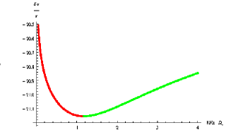
Figure 2: Figure shows the logarithm (to base $10$) of Fractional frequency instability $\frac{\delta\nu}{\nu}$ of a Hydrogen maser in a terrestrial gravitational field as a function of the trap frequency $\Omega_{t}$ expressed in KiloHertz. The major source of the uncertainty in the clock rate in the red part of the curve is the gravitational redshift and in the green part it is the time dilation effect. The optimal choice for the trap frequency occurs at the join of the two parts of the curve, where the fractional instability is $10^{-21}$.

Table 1:        Clock Stability

Clock Type	$\nu_{c}$	Atomic	Gravitational	Limit on
		Mass	Field	Stability
Aluminium	$10^{15}H_{z}$	27	Terrestrial	$10^{-22}$
Aluminium	$10^{15}H_{z}$	27	White Dwarf	$10^{-18}$
Aluminium	$10^{15}H_{z}$	27	Neutron Star	$10^{-14}$
Hydrogen Maser	$10^{9}H_{z}$	1	Terrestrial	$10^{-21}$
Hydrogen Maser	$10^{9}H_{z}$	1	White Dwarf	$10^{-17}$
Hydrogen Maser	$10^{9}H_{z}$	1	Neutron Star	$10^{-13}$
Electron Spin	$10^{13}H_{z}$	1/1836	Terrestrial	$10^{-19}$
Precession
Electron Spin	$10^{13}H_{z}$	1/1836	White Dwarf	$10^{-15}$
Precession
Electron Spin	$10^{13}H_{z}$	1/1836	Neutron Star	$10^{-11}$
Precession
Neutron Spin	$10^{10}H_{z}$	1	Terrestrial	$10^{-21}$
Precession
Neutron Spin	$10^{10}H_{z}$	1	White Dwarf	$10^{-17}$
Precession
Neutron Spin	$10^{10}H_{z}$	1	Neutron Star	$10^{-13}$
Precession				$10^{-13}$

I Acknowledgement

It is a pleasure to thank John Barrow, Miguel Campiglia, Brükner Caslav, Fabio Costa, Nico Giulini, Bei-Lok Hu, H. S. Mani, Igor Pikovski, Hema Ramachandran, Sadiq Rangwala, R. Sorkin, A. M. Srivastava and Magdalena Zych for discussions.

References

- Sobel (2007) D. Sobel, Longitude: The True Story of a Lone Genius Who Solved the Greatest Scientific Problem of His Time (Walker and Company; Reprint edition (October 30, 2007), 2007).
- Ramsey (1983) N. F. Ramsey, Journal of Research of the National Bureau of Standards 88(5), 301 (1983).
- Winkler and Van Flandern (1977) G. M. R. Winkler and T. C. Van Flandern, The Astronomical Journal 82, 84 (1977).
- Lorimer and Kramer (2005) D. R. Lorimer and M. Kramer, Handbook of Pulsar Astronomy (Cambridge University Press, 2005).
- Thomson and Tait (1879) W. Thomson and P. G. Tait, Treatise on Natural Philosophy (Cambridge University Press, 1879).
- Kusch et al. (1940) P. Kusch, S. Millman, and I. I. Rabi, Phys. Rev. 57, 765 (1940), URL http://link.aps.org/doi/10.1103/PhysRev.57.765.
- Chou et al. (2010) C. Chou, D. Hume, T. Rosenbland, and D. Wineland, Science 329, 1630 (2010).
- Hinkley et al. (2013) N. Hinkley, J. A. Sherman, N. B. Phillips, M. Schioppo, N. D. Lemke, K. Beloy, M. Pizzocaro, C. W. Oates, and A. D. Ludlow, Science 341, 1215 (2013).
- Salecker and Wigner (1958) H. Salecker and E. P. Wigner, Phys. Rev. 109, 571 (1958), URL http://link.aps.org/doi/10.1103/PhysRev.109.571.
- Wigner (1957) E. P. Wigner, Rev. Mod. Phys. 29, 255 (1957), URL http://link.aps.org/doi/10.1103/RevModPhys.29.255.
- Barrow (1996) J. D. Barrow, Phys. Rev. D 54, 6563 (1996), URL http://link.aps.org/doi/10.1103/PhysRevD.54.6563.
- Dicke (1953) R. H. Dicke, Phys. Rev. 89, 472 (1953), URL http://link.aps.org/doi/10.1103/PhysRev.89.472.
- Cohen-Tannoudji and Guéry-Odelin (2011) C. Cohen-Tannoudji and D. Guéry-Odelin, Advances in Atomic Physics:An Overview (World Scientific, 2011).
- Schilpp (1970) P. Schilpp, Albert Einstein: Philosopher-scientist (Open Court Publishing Co, US, 1970).
- Campbell et al. (2012) C. J. Campbell, A. G. Radnaev, A. Kuzmich, V. A. Dzuba, V. V. Flambaum, and A. Derevianko, Phys. Rev. Lett. 108, 120802 (2012), URL http://link.aps.org/doi/10.1103/PhysRevLett.108.120802.
- Mössbauer (1958) R. L. Mössbauer, Zeitschrift fur Physik 151, 124 (1958).
- Mukhi (2011) S. Mukhi, Classical and Quantum Gravity 28(15), 153001 (2011).
- Rovelli (2011) C. Rovelli, Classical and Quantum Gravity 28(15), 153002 (2011).
- Sorkin (2009) R. D. Sorkin, J.Phys.Conf.Ser 174, 012018 (2009), URL arXiv:0910.0673.
- Zych et al. (2011) M. Zych, F. Costa, I. Pikovski, and C. Brukner, Nat Commun 2 (2011), URL http://dx.doi.org/10.1038/ncomms1498.
- Pikovski et al. (2013) I. Pikovski, M. Zych, F. Costa, , and C. Brukner (2013), URL http://arxiv.org/abs/1311.1095.
- Sinha and Samuel (2011) S. Sinha and J. Samuel, Classical and Quantum Gravity 28(14), 145018 (2011).
- Sinha (1997) S. Sinha, Physics Letters A 228, 1 (1997).