Revealing the role of electron correlation in sequential double ionization

Abstract

The experimental observations of sequential double ionization (SDI) of Ar [A. N. Pfeiffer et al., Nature Phys. 7, 428 (2011)], such as the four-peak momentum distribution and the ionization time of the first and second electrons, are investigated and reproduced with a quantum model by including and excluding the $e$-$e$ correlation effect. Based on the comparison of experiment and simulation, the role of $e$-$e$ correlation in SDI is discussed. It is shown that the inclusion of $e$-$e$ correlation is necessary to reproduce the momentum distribution of electrons.

Tunneling ionization of atoms, molecules and semiconductors exposed to strong laser fields is one of the most fundamental quantum processes and has been of significant interest over the past several decades review . Theories PPT ; ADK have been well established for single electron ionization based on the Keldysh frame Keldysh . By numerically solving the time-dependent Schrödinger equation (TDSE) with single-active-electron (SAE), Tong and Lin also proposed a more accurate formula Tong , which draws up the well-known Ammosov-Delone-Krainov ionization rate ADK to the numerical simulation via an empirical correction factor, thereby predicting the ionization rate quite precisely.

Nevertheless, for double (or multielectron) ionization, the underlying dynamics become more complicated and have not been fully understood so far. It is generally recognized that two electrons can be ionized either in a non-sequential or sequential process review . In the former mechanism, so-called non-sequential double ionization (NSDI), the $e$-$e$ correlation plays an essential role and the NSDI yield is remarkably enhanced compared with the independent-electron ionization theory Walker . In the latter mechanism, so-called sequential double ionization (SDI), two electrons are released independently step by step, therefore the SDI yield can be simulated by using ionization theory based on SAE. Nevertheless, recent experiments SDI_exp ; Keller2 ; Fleischer have doubted the validity of independent-electron approximation in the SDI regime. Specifically, Fleischer et al. Fleischer reported an angular correlation between the first and second ionization steps. In Ref. SDI_exp , Pfeiffer et al. measured the release time of SDI for Ar by using the attoclock technique Attoclock . The measured release time is in good agreement with the prediction of Tong-Lin’s formula for the first electron, but is much earlier than the theoretical prediction for the second electron. Such a finding has attracted significant interests immediately. Zhou et al. Zhou have reproduced the experimental release time with a classical model by including the $e$-$e$ correlation. Later, Wang et al. XuWang argued that the release time can be successfully explained with a similar classical model by properly adopting the soft-core parameter but excluding the $e$-$e$ correlation, which implies that $e$-$e$ correlation is not essential in SDI.

Even though the classical model is robust, which has been demonstrated extensively in previous investigations Wang2 ; Uzer ; Ho ; XLiu , and also provides a straightforward interpretation with electron trajectory analysis Zhou ; XuWang , the physical picture of SDI is still unclear. Actually, to produce the experimental data, a scaling factor is adopted in Zhou ; XuWang to shift the simulation curve. Strictly speaking, the experiment has not been reproduced. Several curial questions remain: Does the $e$-$e$ correlation play an essential role in SDI? What is its influence and how can its effect be observed? Can we find another indicator to identify the $e$-$e$ correlation, except for ionization times and angular correlation Fleischer ; SDI_exp ? To clarify these questions, we investigate SDI of Ar in an elliptically polarized field by using a quantum model. We show that the $e$-$e$ correlation does affect SDI. It leads to that a small part of the electrons ionize in a correlated way. This effect influences the observed ionization time only slightly, but it affects the overall shape of the momentum distributions.

A complete description of a two-electron system in an elliptically polarized field requires to simulate the motion for each electron in at least two dimensions, which is almost impossible at present WBecker . To overcome the enormous computational challenge, the so-called crapola quantum model Crapora was introduced, which has excellently reproduced the “knee” structure of NSDI Walker ; Gillen . In this model, the total wave function is written,

$$\Psi(\mathbf{r}_{1},\mathbf{r}_{2},t)={\psi_{1}}({\mathbf{r}}_{1},t)\psi_{2}(\mathbf{r}_{2},t)+\psi_{2}(\mathbf{r}_{1},t)\psi_{1}(\mathbf{r}_{2},t),$$ (1)

In the high-intensity elliptically polarized field, the electron is quickly removed from the core and the recollision is significantly suppressed. Then we can assume that the overlap between the two electrons is sufficiently small for the exchange term and can be negligible in comparison to the Coulomb repulsion. Thus only the first term needs to be considered. The time evolutions of the first (i.e., outer electron, $\psi_{1}(\mathbf{r}_{1},t)$) and second (i.e., inner electron, $\psi_{2}({\mathbf{r}}_{2},t)$) electrons are described by

$$i\frac{\partial\psi_{n}(\mathbf{r}_{n},t)}{\partial t}=[-\frac{\nabla^{2}}{2}+V_{n}(\mathbf{r}_{n},t)+V_{\rm int}(\mathbf{r}_{n},t)]\psi_{n}(\mathbf{r}_{n},t),$$ (2)

where atomic units (a.u.) are adopted and $\mathbf{r}_{n}$ denotes two-dimensional coordinates $(x_{n},y_{n})$, $n=1,2$ refer to the first and second electrons, V${}_{\rm int}=\mathbf{r}_{n}\cdot~{}{\mathbf{E}}(t)$ and ${\mathbf{E}}(t)=E_{0}\exp(-t^{2}/\tau^{2}/2)[\epsilon/\sqrt{\epsilon^{2}+1}\cos{(\omega~{}t+\phi_{0})}\hat{\mathbf{x}}+1/\sqrt{\epsilon^{2}+1}\sin(\omega~{}t+\phi_{0})\hat{\mathbf{y}}]$ is the driving laser field. $\epsilon$, $\tau$ and $\phi_{0}$ refer to the ellipticity, duration and carrier-envelope phase (CEP), respectively. In the crapola quantum model, the first electron was assumed to move in a static effective potential due to the nucleus and inner electrons, i.e., $V_{1}(\mathbf{r}_{1},t)=-1/\sqrt{\mathbf{r}_{1}^{2}+a_{1}}$. For the second electron, the interaction with the first electron was taken into account. Thus, V₂ includes a static effective potential due to the nucleus plus a time-dependent potential due to the first electron,

$$V_{2}(\mathbf{r}_{2},t)=\frac{-2}{\sqrt{a_{2}+\mathbf{r}_{2}^{2}}}+\int d\mathbf{r}_{1}\frac{\alpha\psi_{1}^{*}(\mathbf{r}_{1},t)\psi_{1}(\mathbf{r}_{1},t)}{\sqrt{\beta+(\mathbf{r}_{1}-\mathbf{r}_{2})^{2}}}.$$ (3)

where $a_{1}$, $a_{2}$ and $\beta$ are the soft-core parameters for the e-ion and $e$-$e$ interactions. The second electron is correlated with the first one through the time-dependent term of Eq. 3. We could include or exclude the $e$-$e$ correlation by setting $\alpha=1$ or 0. In the former case, we adjust the $e$-$e$ correlation strength by changing $\beta$ to identify its influence. Note that in the crapola quantum model, the correlation of the first electron on the second is taken into account while its counteractive, i.e., the time-dependent potential of the second electron on the first electron, is not explicitly included. In order to remedy this seemingly unreasonable treatment, we performed other calculations where the time-dependent potential of the second electron on the first electron is also explicitly taken into account. Thus, the potential for the first electron is

$$V_{1}(\mathbf{r}_{1},t)=\frac{-1}{\sqrt{a_{1}+\mathbf{r}_{1}^{2}}}+\int d\mathbf{r}_{2}\frac{\alpha\psi_{2}^{*}(\mathbf{r}_{2},t)\psi_{2}(\mathbf{r}_{2},t)}{\sqrt{\beta+(\mathbf{r}_{1}-\mathbf{r}_{2})^{2}}}.$$ (4)

We call this method revised correlation model in this work.

We employ the split-operator method MFeit to numerically solve Eq. (2). Like in Ref. XTong , the two-dimensional space of each electron is partitioned into two regions: the outer region A {$|{r_{n}}|>a$} and the inner region B {$|{r_{n}}|<a$} with $a$=100 a.u. In the inner region, the wave function is propagated exactly in the presence of combination of the Coulombic potential and the laser field. In the outer region, the wave function is propagated under the Volkov Hamiltonian analytically and the final momentum spectra of the first electron $C_{1}(\mathbf{p}_{1})$ and the second $C_{2}(\mathbf{p}_{2})$ are obtained from the wave function in this region XTong . The inner and the outer regions are smoothly divided by a splitting techniqueXTong . The ground states of the two electrons are obtained by imaginary-time method. In order to identify how $e$-$e$ correlation affects SDI, calculations were performed by treating the time-dependent potential of $e$-$e$ interaction in different ways as mentioned above, i.e., including (revised correlation model) and excluding (uncorrelated model) it for both electrons, and the crapola model. The data shown below are the results from the uncorrelated and revised correlation model, while the results from the crapola model is shown in the supplemental material for comparison Supplemental .

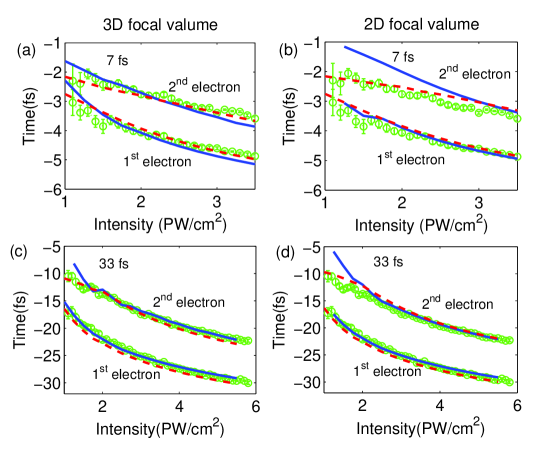
Figure 1: (Color online) Release times of the first and second electrons. (a) and (b) for the 7-fs pulse, (c) and (d) for the 33-fs pulse. The peak of pulse is at time zero. The left and right columns correspond to 3D and 2D focal volumes. Circles with error bars are experimental data SDI_exp . Solid lines show the simulation results using uncorrelated model,i.e., $\alpha=0$, $a_{1}=0.4$, $a_{2}=1.0$. Dashed lines show the simulation result with revised correlation model, i.e., $\alpha=1$, $\beta=4$, $a_{1}=0.18$, $a_{2}=1.04$.

Figure 1 shows the simulated ionization times of the first and second electrons for the 7-fs and 33-fs pulses. The central wavelengths of the 7-fs and 33-fs pulses are 740 nm and 780 nm and the ellipticities are 0.78 and 0.77, respectively. For the 7-fs pulse, four CEP values, 0, $\pi$ and $\pm\pi/2$, are adopted and the final simulation results are averaged over the CEP. For a comparison with experimental data, the intensity profile of the laser focus, the density distribution of the atoms in the gas jet, and the geometrical overlap of the focus and the gas jet need to be considered. Because of uncertainties of these parameters in experiment SDI_exp , a 3D focal volume averaging (assumption of constant gas density across the entire 3-dimensional Gaussian beam focal ) and a 2D focal volume averaging (assumption of constant gas density only at the waist of the beam and zero gas density otherwise, indicating a gas jet small compared to the Rayleigh range of the laser focus) are tested here. We first analyze the result for the 3D focal volume averaging. As shown in Fig. 1(a), the simulated ionization time agrees well with the experimental data for both electrons, regardless of the $e$-$e$ correlation being excluded (solid lines) or included (dashed lines). For the 2D focal volume averaging, as shown in Fig. 1(b), both calculations also agree very well with the experimental data for the first electron. For the second electron, the calculations with uncorrelated model agree with the experimental data at the high laser intensity range while deviates slightly at the low laser intensity range. The calculations with revised correlation model agree better with the experimental data at low intensity.

Figure 1(c) and (d) show the simulation results for the 33-fs pulse by assuming a 3D and 2D focal configuration, respectively. One can see that the $e$-$e$ correlation indeed influences the ionization time, but the influence is slight. Additionally, the absolute values of the ionization times depend also on the details of the focal geometry, which is unknown in experiment. The ionization times simulated by uncorrelated model, revised correlation model and crapola model (see Fig. S2 in Supplemental ) all can explain the experiment if accounting for the uncertainties in experiment. Thus, it is difficult to judge the role of $e$-$e$ correlation in SDI based the ionization time. These ionization times read in the experiments and our calculations are integral signals, which have erased the details in SDI, obstructing our way on revealing the role of $e$-$e$ correlation in SDI. Therefore, another indicator which keeps more details of the ionization process and robust against uncertainties in the focal volume averaging, is needed to identify the role of $e$-$e$ correlation.

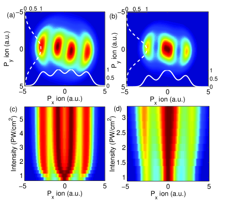
Figure 2: (Color online) Two-dimensional momentum distribution for 33-fs pulse at high [(a): 3 PW/cm²] and low [(b): 1 PW/cm²] intensities. The solid and dashed lines show the projection onto the x and y axis. (c) and (d): Momentum distribution of Ar²⁺ ion along the x axis as a function of laser intensity for the 33-fs and 7-fs pulses. Electron correlation is taken into account and 3D focal volume averaging is applied.

Figure 2(a) and (b) show the two-dimensional momentum distribution of Ar²⁺ for 33-fs pulse at 3 PW/cm² and 1 PW/cm², respectively. Here the $e$-$e$ correlation is taken into account by using the revised correlation model and 3D focal volume configure is considered. By projecting onto the major axis of the ellipse (y axis), the momentum distribution is close to Gaussian, whereas along the minor axis (x axis), it displays 3 peaks at low intensity and 4 peaks at high intensity. The outer two peaks correspond to electrons that are emitted into parallel direction and the inner peaks correspond to antiparallel electron emission SDI_exp ; Maharjan . Figure 2(c) shows the momentum distribution along the minor axis as a function of laser intensity. As shown in this figure, the inner band gradually expands with increasing the intensity and bifurcates into two branches from 1.5 PW/cm². While for the 7-fs pulse, as shown in Fig. 2(d), the inner band also expands with increasing the intensity but does not bifurcate over the intensity range considered in this work. All these features agree well with the experiment SDI_exp . Simulations are also performed by using the uncorrelated model and crapola model. The ion momentum distributions do not display remarkable difference except that the depth of valley between the inner and outer peaks change slightly (see Figs. S3 and S4 in Supplemental ).

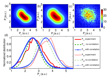
Figure 3: (Color online) Correlation spectrum of radial momentum P_r1 and P_r2 for the 7-fs pulse with peak intensity 3 PW/cm². Uncorrelated model and revised correlation model are used in (a) and (b). (c) experimental correlation spectrum. (d) reduced spectrum of P_r1 and P_r2. Here, the 3D focal volume averaging is applied.

To get a deeper insight into the role of $e$-$e$ correlation, we investigate the correlation spectrum of the radial momentum, which is defined as P${}_{r}=\sqrt{[(\epsilon^{2}+1)/\epsilon^{2}]P_{x}^{2}+(\epsilon^{2}+1)P_{y}^{2}}$, and P_r1 and P_r2 are the radial momenta of the first and the second electrons, respectively. Figures 3(a) and (b) show the simulation results by using the uncorrelated model and the revised correlation model for the 7-fs pulse. Figure 3(c) presents the correlation spectrum observed in the experiment. The difference between Figs. 3(a) and (b) is remarkable. The distribution including $e$-$e$ correlation is fatter than that excluding $e$-$e$ correlation. The result including $e$-$e$ correlation agrees better with the experimental observations. This feature can be more clearly seen in the reduced spectra, which are respectively obtained from the momentum spectra of the first electron $C_{1}(\mathbf{p}_{1})$ and the second electron $C_{2}(\mathbf{p}_{2})$. As shown in Fig. 3(d), for both electrons, the widths of the spectra excluding $e$-$e$ correlation are narrower than the experimental data. While for the spectra including $e$-$e$ correlation, the widths are in agreement with the experimental data. In order to further confirm that the broadening of the reduced spectra originates from the $e$-$e$ correlation, we performed other calculations where the strength of $e$-$e$ correlation is enhanced by decreasing the soft-parameter $\beta$. As shown in the supplementary material Supplemental , the reduced spectra become wider for both electrons for a smaller value of $\beta$. Note that a fat radial momentum distribution is also obtained by the crapola model Supplemental . These results indicate that SDI indeed is influenced by $e$-$e$ correlation and this influence leaves imprint on the electron momentum spectra.

As shown in Figs. 3(a) and 3(b), the peaks of the momentum spectra do not change dramatically when $e$-$e$ correlation is excluded or included. Therefore the mean value of radial momentum is not dramatically influenced by $e$-$e$ correlation. In the attoclock experiment SDI_exp , the ionization time is extracted from the radial momenta. Therefore, the influence of the $e$-$e$ correlation on the averaged ionization time is not very effective. Similar remarks also can be observed for the 33-fs pulse. This feature also explains the puzzle why the ionization time can be reproduced with the classical model either including or excluding the $e$-$e$ correlation Zhou ; XuWang .

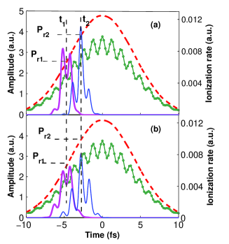
Figure 4: (Color online) Ionization rate of the first (bold magenta lines) and second (thin blue lines) electrons as a function of time for the 7-fs pulse with peak intensity of 3 PW/cm². Uncorrelated model and revised correlation model are adopted in (a) and (b). The solid lines with dots and the dashed lines represent the vector potential of the laser field and the radial momentum, respectively

The origin of the broadening of the reduced momentum spectra is related to the time intervals when the first and the second ionizations occur. Figure 4(a) shows the ionization rate as a function of time at 3 PW/cm² for the 7-fs pulse. The bold and thin solid lines correspond to the first and second electrons without $e$-$e$ correlation. Because the laser intensity is much higher than the saturation intensity, the ionization is confined in a single cycle around t₁ and t₂ at the ascending part of the pulse, respectively. After ionization, the electrons are accelerated by the laser field and finally released with a momentum of P_r1 and P_r2 as shown in Fig. 4(a). But because of no correlation, the second electron is not freed when $t<t_{1}$ and the first ionization process is already finished when $t\geq t_{2}$. In contrast, when the $e$-$e$ correlation is accounted for [Fig. 4(b)], the centra of the ionization time ($t_{1}$ and $t_{2}$) for both electrons almost do not change. This is consistent with the above results that the ionization time is not effectively influenced by the $e$-$e$ correlation. However, as shown in Fig. 4(b), when $t<t_{1}$, small percentage of the second electron starts to be released and also small percentage of the first electron is released at $t\geq t_{2}$. Consequently, the ionization windows of the first and second ionization processes become broader than those excluding the $e$-$e$ correlation. The long ionization window broadens the width of the momentum distribution. Moreover, because the first electron quickly moves away after ionization, its correlation with the second electron drops quickly. Only a small percentage of the first and second electrons can be ionized in a correlated way. By increasing the $e$-$e$ correlation, larger percentage of the electrons can be ionized in a correlated way and the momentum spectra will be further broadened as shown in the supplementary material Supplemental . Therefore, the width of the momentum spectrum, which is closely related to the ionization window, exhibits the faint details of $e$-$e$ correlation in SDI.

In conclusion, SDI of Ar subjected to elliptically polarized pulses is investigated using quantum models. It is shown that the $e$-$e$ correlation indeed slightly shifts the ionization time, but its influence is not crucial to explain the experiment SDI_exp . Moreover, uncertainties in the focal volume averaging also influence the apparent ionization times. It is difficult to decisively reveal the role of $e$-$e$ correlations based on the ionization timing data alone. However, our simulations show that the $e$-$e$ correlation broadens the time windows for the first and second ionizations. Though this effect could not be distinguished in the ionization time of the second electron, it affects the momentum distribution. The signature of $e$-$e$ correlation can be identified in the width of the electron momentum distribution. By comparing with the experiment SDI_exp , the width of the electron momentum distribution for 7-fs pulse agrees well with the simulation including fair $e$-$e$ correlation, which indeed indicates the exist of $e$-$e$ correlation in SDI. The subtle features of momentum distribution require further experimental measurements with low noise and high accuracy.

References

- (1) See recent reviews, V. S. Popov, Phys. Uspekhi 47, 855 (2004); W. Becker, X. J. Liu, P. J. Ho, J. H. Eberly, Rev. Mod. Phys. 84, 1011 (2012).
- (2) M. V. Ammosov, N. B. Delone and V. P. Krainov, Sov. Phys. JETP 64, 1191 (1986).
- (3) A. M. Perelomov, V. S. Popov, M. V. Terentev, Sov. Phys. JETP 23, 924 (1966).
- (4) L. V. Keldyshi, Sov. Phys. JETP 20, 1307 (1965).
- (5) X. M. Tong, C. D. Lin, J. Phys. B 38, 2593 (2005).
- (6) B. Walker, et al., Phys. Rev. Lett. 73, 1227 (1994).
- (7) A. N. Pfeiffer, C. Cirelli, M. Smolarski, R. Dorner, U. Keller, Nature Phys. 7, 428 (2011).
- (8) A. N. Pfeiffer, et al., New. J. Phys. 13, 093008 (2011).
- (9) A. Fleischer, et al., Phys. Rev. Lett. 107, 113003 (2011).
- (10) P. Eckle, et al., Nature Phys. 4, 565 (2008); P. Eckle, et al., Science 322, 1525 (2008).
- (11) Y. M. Zhou, et al., Phys. Rev. Lett. 109, 053004 (2012); ibid., Phys. Rev. A 86, 043427 (2012).
- (12) X. Wang, J. Tian, A. N. Pfeiffre, C. Cirelli, U. Keller, J. H. Eberly, arXiv:1208.1516; X. Wang, J. H. Eberly, J. Chem. Phys. 137, 22A542 (2012); J. H. Eberly, Invited talk on the Workshop on Super Intense Laser-Atom Physics, Spe. 2012, Suzhou, China.
- (13) X. Wang, J. H. Eberly, Phys. Rev. Lett. 103, 103007 (2009).
- (14) F. Mauger, C. Chandre, T. Uzer, Phys. Rev. Lett. 105, 083002 (2010); ibid., 104, 043005 (2010).
- (15) P. J. Ho, et al., Phys. Rev. Lett. 94, 093002 (2005); ibid., 97, 083001 (2006); S. L. Haan, et al., Phys. Rev. Lett. 97, 103008 (2006).
- (16) W. Quan, et al., Phys. Rev. Lett. 103, 093001 (2009); H. Liu, et al., Phys. Rev. Lett. 109, 093001 (2012).
- (17) W. Becker, H. Rottke, Contemp. Phys. 49, 199 (2008).
- (18) J. B. Watson, et al., Phys. Rev. Lett. 78, 1884 (1997).
- (19) G. D. Gillen, M. A. Walker, L. D. Van Woerkom, Phys. Rev. A 64, 043413 (2001). Note that the “knee” structure of Mg in circularly polarized field reported in this work can be simulated by using the crapola model.
- (20) M. Feit, J. Fleck, Jr., and A. Steiger, J. Comput. Phys. 47, 412 (1982).
- (21) X. M. Tong, K. Hino, and N. Toshima, Phys. Rev. A 74, 031405(R) (2006)
- (22) P. Q. Wang, A. Max Sayler, K. D. Garnes, B. D. Esry, I. Ben-Itzhak, Opt. Lett. 30, 664 (2005)
- (23) See the supplementary material.
- (24) C. M. Maharjan, et al., Phys. Rev. A 72, 041403(R) (2005).