Optimal Control with Noisy Time

Abstract

This paper examines stochastic optimal control problems in which the state is perfectly known, but the controller’s measure of time is a stochastic process derived from a strictly increasing Lévy process. We provide dynamic programming results for continuous-time finite-horizon control and specialize these results to solve a noisy-time variant of the linear quadratic regulator problem and a portfolio optimization problem with random trade activity rates. For the linear quadratic case, the optimal controller is linear and can be computed from a generalization of the classical Riccati differential equation.

I Introduction

Effective feedback control often requires accurate timekeeping. For example, finite-horizon optimal control problems generally result in policies that are time-varying functions of the state. However, chronometry is imperfect and thus feedback laws are inevitably applied at incorrect times. Little appears to be known about the consequences of imperfect timing on control [1, 2, 3]. This paper addresses optimal control with temporal uncertainty.

A stochastic process can be time-changed by replacing its time index by a monotonically increasing stochastic process [4]. Time-changed stochastic processes arise in finance, since changing the time index to a measure of economically relevant events, such as trades, can improve modeling [5, 6, 7]. This new time index is, however, stochastic with respect to “calendar” time.

We suspect that similar notions of stochastic time changing may facilitate the study of time estimation and movement control in the nervous system. Biological timing is subject to noise and environmental perturbation [8]. Furthermore, humans rationally exploit the statistics of their temporal noise during simple timed movements, such as button pushing [9] and pointing [10]. To analyze more complex movements, a theory of feedback control that compensates for temporal noise seems desirable.

Within control, the most closely related work to the present paper deals with analysis and synthesis of systems with uncertain sampling times. The study of uncertain sampling times has a long history in control [11], and is often motivated by problems of clock jitter [12, 13] or network delays [14]. In these works, control inputs are sampled at known times and held over unknown intervals. To derive the dynamic programming principle in this paper, system behavior is analyzed for control inputs held over random intervals, bearing some similarity to optimal control with random sampling [15]. Fundamentally, however, studies of sampling uncertainty assumes that an accurate clock can measure the sample times; the present work relaxes this assumption.

Other aspects of imperfect timing have been addressed in control research to a more limited extent. For example, the importance of synchronizing clocks in distributed systems seems clear [16, 17], but more work is needed to understand the the implications of asynchronous clock behavior on common control issues, such as stability [18] and optimal performance [19].

This paper focuses on continuous-time stochastic optimal control with perfect state information, but a stochastically time-changed control process. Dynamic programming principles for general nonlinear stochastic control problems are derived, based on extensions of the classical Hamilton-Jacobi-Bellman equation. The results apply to a wide class of stochastic time changes given by strictly increasing Lévy processes. The dynamic programming principles are then specialized to give explicit solutions to time-changed versions of the finite-horizon linear quadratic regulator and a portfolio optimization problem.

Section II defines the notation used in the paper, states the necessary facts about Lévy, and defines the class of noisy clock models used. The main results on time-changed diffusions and optimal control are given in Section III. The results are proved in Sections IV with supplementary arguments given in the appendices. Sections V and VI discuss future work and conclusions, respectively.

II Preliminaries

After establishing notation and reviewing Lévy processes, this section culminates in the construction of Lévy-process-based clock models upon which the remainder of the theory of this paper is built.

II-A Notation

The norm symbol, $\|\cdot\|$, is used to denote the Euclidean norm for vectors and the Frobenius norm for matrices.

For a set $S$, its closure is denoted by $\overline{S}$.

The spectrum of matrix $A$ is denoted by $\mathrm{spec}(A)$.

The Kronecker product is denoted by $\otimes$, while the Kronecker sum is denoted by $\oplus$:

$$A\oplus B=A\otimes I+I\otimes B.$$

The vectorization operation of stacking the columns of a matrix is denoted by $\mathrm{vec}$.

A function $h:\mathbb{R}\times\mathbb{R}^{n}\to\mathbb{R}$ is in $\mathcal{C}^{1,2}$ if $h(s,x)$ is continuously differentiable in $s$, twice continuously differentiable in $x$. The function $h$ is said to satisfy a polynomial growth condition, if in addition, there are constants $K$ and $q$ such that

$$|h(s,x)|,\>\left|\frac{\partial h(s,x)}{\partial s}\right|,\>\left|\frac{\partial h(s,x)}{\partial x_{i}}\right|,\>\left|\frac{\partial^{2}h(s,x)}{\partial x_{i}\partial x_{j}}\right|\leq K\left(1+\|x\|^{q}\right),$$

for $i,j=1,\ldots n$, and all $x\in\mathbb{R}^{n}$. In this case, $h\in\mathcal{C}_{p}^{1,2}$ is written.

Stochastic processes will be denoted as $\zeta_{t}$, $X_{s}$, etc., with time indices as subscripts. Occasionally, processes with nested subscripts will be written with parentheses, e.g. $\zeta_{\tau_{s}}=\zeta(\tau_{s})$. Similarly, the elements of a stochastic vector will be denoted as $X_{1}(s)$.

Functions that are right-continuous with left-limits will be called càdlàg, while functions that are left-continuous with right-limits will be called càglàd.

II-B Background on Lévy Processes

Basic notions from Lévy processes required to define the general class of clock models are now reviewed. The definitions and results can be found in [20].

A real-valued stochastic process $Z_{s}$ is called a Lévy process if

• $Z_{0}=0$ almost surely (a.s.).

• $Z_{s}$ has independent, stationary increments: If $0\leq r\leq s$, then $Z_{r}$ and $Z_{s}-Z_{r}$ are independent and $Z_{s}-Z_{r}$ has the same distribution as $Z_{s-r}$.

• $Z_{s}$ is stochastically continuous: For all $a>0$ and all $r\geq 0$, $\lim_{r\to s}\mathbb{P}(|Z_{s}-Z_{r}|>a)=0$.

It will be assumed that Lévy processes in this paper are right-continuous with left-sided limits, i.e. they are càdlàg. No generality is lost since, for every Lévy process, $Z_{t}$, there is a càdlàg Lévy process, $\tilde{Z}_{t}$, such that $Z_{t}=\tilde{Z}_{t}$ for almost all $t$.

Some of the more technical arguments rely on the notion of Poisson random measures, which will now be defined. Let $\mathcal{B}$ be the Borel subsets of $\mathbb{R}$ and let $(\Omega,\Sigma,\mathbb{P})$ be a probability space. A Poisson random measure is a function $N:[0,\infty)\times\mathcal{B}\times\Omega\to\mathbb{N}\cup\{\infty\}$, such that

• For all $s\geq 0$ and $\omega\in\Omega$, $N(s,\cdot,\omega)$ is a measure.

• For all disjoint Borel subsets $A,B\in\mathcal{B}$ such that $0\notin\overline{A}$ and $0\notin\overline{B}$, $N(\cdot,A,\cdot)$ and $N(\cdot,B,\cdot)$ are independent Poisson processes.

Typically, the $\omega$ argument will be dropped, and it will be implicitly understood that $N(s,A)$ denotes a measure-valued stochastic process.

The following relationship between Lévy processes and Poisson random measures will be used in several arguments. For a Lévy process, $Z_{s}$, with jumps denoted by $\Delta Z_{s}$, there is a Poisson random measure that counts the number of jumps into each Borel set $A$ with $0\notin\overline{A}$:

$$N(s,A)=\left|\{\Delta Z_{r}\in A:0\leq r\leq s\}\right|.$$

Subordinators. A monotonically increasing Lévy process, $\tau_{s}$, is called a subordinator. The following properties of subordinators will be used throughout the paper.

• Laplace Exponent: There is function, $\psi$, called the Laplace exponent, defined by

  $$\psi(z)=bz+\int_{0}^{\infty}\left(1-e^{-zt}\right)\lambda(dt),$$ (1)

  such that

  $$\mathbb{E}\left[e^{-z\tau_{s}}\right]=e^{-s\psi(z)}\qquad\textrm{for all}\qquad z\geq 0.$$ (2)

  Here $b\geq 0$ and the measure satisfies $\int_{0}^{\infty}\min\{t,1\}\lambda(dt)<\infty$. The measure $\lambda$ is called a Lévy measure. The pair $(b,\lambda)$ is called the characteristics of $\tau_{s}$.

• Lévy-Itô Decomposition: There is a Poisson random measure $N$ such that

  $$\tau_{s}=bs+\int_{0}^{\infty}tN(s,dt).$$

  Furthermore, if $A\subset(0,\infty)$ is a Borel set such that $0\notin\overline{A}$, then $\mathbb{E}[N(1,A)]=\lambda(A)$.

The function, $\psi$, is called the Laplace exponent because (2) is the Laplace transform of the distribution of $\tau_{s}$.

For control problems, simpler formulas will often result from replacing $\psi$ with the function $\beta(z)=-\psi(-z)$. Note then, that $\beta$ has the form

$$\beta(z)=bz+\int_{0}^{\infty}\left(e^{zt}-1\right)\lambda(dt).$$ (3)

Define $r_{\max}$ by

$$r_{\max}=\sup\left\{r:\int_{1}^{\infty}e^{rt}\lambda(dt)\right\}$$

and define the domain of $\beta$ as

$$\mathrm{dom}(\beta)=\{z\in\mathbb{C}:\mathrm{Re}\>z<r_{\max}\}.$$

Note that $\int_{1}^{\infty}\lambda(dt)<\infty$ implies that $r_{\max}\in[0,\infty]$.

The function $\beta$ is used to construct optimal solutions for the linear quadratic problem, as well as the portfolio problem below. The main properties are given in the following lemma, which is proved in Appendix B.

Lemma 1

For all $z\in\mathrm{dom}(\beta)$, the function $\beta$ is analytic at $z$, and

$$\mathbb{E}\left[e^{z\tau_{s}}\right]=e^{s\beta(z)}.$$ (4)

Furthermore, if $A$ is a square matrix with $\mathrm{spec}(A)\subset\mathrm{dom}\beta$, then

$$\beta(A)=bA+\int_{0}^{\infty}\left(e^{At}-I\right)\lambda(dt)$$ (5)

is well defined and

$$\mathbb{E}\left[e^{A\tau_{s}}\right]=e^{s\beta(A)}.$$ (6)

Since $\beta$ is analytic, several methods exist for numerically computing the matrices $\beta(A)$ [21]. In some special cases, as discussed below, $\beta(A)$ may be computed using well-known matrix computation methods.

Example 1

The simplest non-trivial subordinator is the Poisson process $N_{t}$, which is characterized by

$$\mathbb{P}(N_{t}=k)=e^{-\gamma t}\frac{(\gamma t)^{k}}{k!},$$

where $\gamma>0$ is called the rate constant. Its Laplace exponent is given by $\psi(z)=\gamma-\gamma e^{-z}$, which is found by computing the expected value directly. The characteristics are $(0,\gamma\delta(t-1))$. In this case, $\mathrm{dom}(\beta)=\mathbb{C}$, and $\beta(A)=\gamma e^{A}-\gamma I$, which can be computed from the matrix exponential.

Example 2

The gamma subordinator, which is often used to model “business time” in finance [22, 23], has increments distributed as gamma random variables. It has Laplace exponent $\psi(z)=\delta\log(1+z/\gamma)$ with characteristics $b=0$ and $\lambda(dt)=\delta e^{-\gamma t}t^{-1}dt$. Thus $\beta(z)=-\delta\log(1-z/\gamma)$, $\mathrm{dom}(\beta)=\{z\in\mathbb{C}:\mathrm{Re}\>z<\gamma\}$, and matrix function $\beta(A)=-\delta\log\left(I-\gamma^{-1}A\right)$ may be computed from the matrix logarithm.

Why Lévy Processes? In the next subsection, the clock model in this paper will be constructed from a subordinator $\tau_{s}$. The motivation for using Lévy processes will be explained. Consider a continuous-time noisy clock, $c_{s}$ which is sampled with period $\delta$. A natural model might take the form

$$c_{\delta(k+1)}=c_{\delta k}+\delta+n(k,\delta),$$ (7)

where $n(j,\delta)$ are random variables. In this case, the clock increments consist of a deterministic step of magnitude $\delta$ plus a random term.

If $c_{s}$ is a Lévy process, then by definition, all of the increments $c_{\delta(k+1)}-c_{\delta k}$ are independent and identically distributed. Thus, the decomposition in (7) holds with $n(k,\delta)=c_{\delta(k+1)}-c_{\delta k}-\delta$. If $c_{s}$ were not a Lévy process, then (7) may hold for some particular $\delta$, but there might be another period, $\delta^{\prime}<\delta$, for which the decomposition fails. The Lévy process assumption will guarantee that the clocks are well-behaved when taking continuous time limits (i.e. $\delta\downarrow 0$).

II-C Clock Models

Throughout the paper, $t$ will denote the time index of the plant dynamics, while $s$ will denote the value of clock available to the controller. Often, $t$ and $s$ will be called plant time and controller time, respectively. The interpretation of $s$ and $t$ varies depending on context. In biological motor control, $t$ would denote real time, since the limbs obey Newtonian mechanics with respect to real-time, while $s$ would denote the internal representation of time. For the portfolio problem studied in Subsection III-B, an opposite interpretation holds. Here, the controller (an investor) can accurately measure calendar time, but price dynamics are simpler with respect a different index, “business time”, which represents the progression of economic events [6, 7, 5]. Thus, $s$ would denote calendar time, while $t$ would denote business time, which might not be observable.

The relationship between $s$ and $t$ will be described stochastically. Let $\tau_{s}$ be a strictly increasing subordinator. In other words, if $s<s^{\prime}$ then $\tau_{s}<\tau_{s^{\prime}}$ a.s. (Note that any subordinator can be made to be strictly increasing by adding a drift term $bs$ with $b>0$.) The process $\tau_{s}$ will have the interpretation of being the amount of plant time that has passed when the controller has measured $s$ units of time. The process $\zeta_{t}$ will be an inverse process that describes how much time the controller measures over $t$ units of plant time. Formally, $\zeta_{t}$ is defined by

$$\zeta_{t}=\inf\{\sigma:\tau_{\sigma}\geq t\}.$$ (8)

Note that $\zeta(\tau_{s})=s$ a.s. Indeed, $\zeta(\tau_{s})=\inf\{\sigma:\tau_{\sigma}=\tau_{s}\}$, by definition. Since $\tau_{s}$ is right continuous and strictly increasing, a.s., it follows that $\zeta_{\tau_{s}}=s$, a.s.

Example 3

The case of no temporal uncertainty corresponds to $\tau_{s}=s$ and $\zeta_{t}=t$. The Laplace exponent of $\tau_{s}$ is computed directly as $\psi(z)=z$ and the characteristics are $(1,0)$. Here $\mathrm{dom}(\beta)=\mathbb{C}$.

Example 4

A more interesting temporal noise model, also used as a “business time” model [24], is the inverse Gaussian subordinator. Fix $\gamma>0$ and $\delta>0$. Let $C_{t}=\gamma t+W_{t}$, where $W_{t}$ is a standard unit Brownian motion. The inverse Gaussian subordinator is given by

$$\tau_{s}=\inf\{t:C_{t}=\delta s\},$$

with Laplace exponent $\psi(z)=\delta(\sqrt{\gamma^{2}+2z}-\gamma)$. Here $b=0$ and $\lambda$ is given by

$$\lambda(dt)=\frac{\delta}{\sqrt{2}\Gamma(1/2)}e^{-\frac{1}{2}\gamma^{2}t}t^{-\frac{3}{2}}dt,$$

where $\Gamma$ is the gamma function. Here, $\mathrm{dom}(\beta)$ corresponds to $\mathrm{Re}\>z<\gamma^{2}/2$ and $\beta(A)=\delta\left(\gamma I-\sqrt{\gamma^{2}I-2A}\right)$, which can be computed from the matrix square root. It can be shown that the inverse process is given by

$$\zeta_{t}=\sup\left\{\delta^{-1}C_{\sigma}:0\leq\sigma\leq t\right\}.$$

See Figure 1.

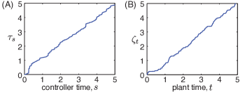
Figure 1: (A). The inverse Gaussian subordinator, $\tau_{s}$, with $\gamma=\delta=2$. The process was simulated by generating independent inverse Gaussians using the method from [25]. (B) The inverse process, $\zeta_{t}$. Note that the graph of $\zeta_{t}$ can be found from the graph of $\tau_{s}$ by simply switching the axes.

In the preceding example, the process $\tau_{s}$ has jumps, but the inverse, $\zeta_{t}$, is continuous. The next proposition generalizes this observation for any strictly increasing subordinator, $\tau_{s}$.

Proposition 1

The process $\zeta_{t}$ is continuous almost surely.

Proof:

Fix $\epsilon>0$ and $t\geq 0$. Set $s=\zeta_{t}$. Strict monotonicity of $\tau_{s}$ implies that $[\tau_{\max\{s-\epsilon,0\}},\tau_{s+\epsilon}]$ is a nonempty interval, a.s. The inverse property of $\zeta_{t}$ implies (almost surely) that $t\in[\tau_{\max\{s-\epsilon,0\}},\tau_{s+\epsilon}]$ and $\zeta_{t^{\prime}}\in[\max\{s-\epsilon,0\},s+\epsilon]$ for all $t^{\prime}\in[\tau_{\max\{s-\epsilon,0\}},\tau_{s+\epsilon}]$.      

III Main Results

This section presents the main results of the paper. First, given an Itô process, $Y_{t}$, a representation of the time-changed process $X_{s}=Y(\tau_{s})$ as a semimartingale with respect to controller time, $s$, is derived. This representation is then used to derive a general dynamic programming principle for control problems with noisy clocks. As an example, the dynamic programming principle is used to solve a simple portfolio optimization problem under random trade activity rates. Finally, the dynamic programming method is used to solve a noisy-time variant of the linear quadratic regulator problem. All proofs are given in Section IV.

III-A Time-Changed Stochastic Processes

This section gives a basic representation theorem for time-changed stochastic processes that will be vital for dynamic programming proofs. The theorem is proved in Subsection IV-A.

Let $W_{t}$ be a Brownian motion with $\mathbb{E}[W_{t}W_{t}^{\mathsf{T}}]=tI$. Let $Y$ be a stochastic process defined by

$$dY_{t}=F_{t}dt+G_{t}dW_{t},$$ (9)

where $F_{t}$ and $G_{t}$ are $\mathcal{F}_{t}^{W}$ predictable processes, where $(\mathcal{F}_{t}^{W})_{t\geq 0}$ is the $\sigma$-algebra generated by $W_{t}$. Furthermore, assume that $F_{t}$ and $G_{t}$ are left-continuous with right-sided limits.

Let $\mathcal{F}^{\tau,W}=(\mathcal{F}_{s}^{\tau,W})_{s\geq 0}$ be the smallest filtration such that for all $r\in[0,s]$ and all $t\in[0,\tau_{s}]$ both $\tau_{r}$ and $W_{t}$ are measurable.

Theorem 1

Let $\tau_{s}$ be a subordinator characterized by $(b,\lambda)$. If the terms of (9) satisfy

• $\int_{0}^{\tau_{S}}\|F_{t}\|dt<\infty$ almost surely and

• $\mathbb{E}\left[\int_{0}^{\tau_{S}}\|G_{t}\|^{2}dt\right]<\infty$,

then the time-changed process $X_{s}=Y(\tau_{s})$ is an $\mathcal{F}^{\tau,W}$ semimartingale given by

$$X_{s}=X_{0}+b\int_{0}^{s}F(\tau_{r^{-}})dr+\sqrt{b}\int_{0}^{s}G(\tau_{r^{-}})d\tilde{W}_{r}+\\ \sum_{0\leq r\leq s}\left(\int_{\tau_{r^{-}}}^{\tau_{r}}F_{t}dt+\int_{\tau_{r^{-}}}^{\tau_{r}}G_{t}dW_{t}\right).$$ (10)

Here $\tilde{W}_{s}$ is an $\mathcal{F}^{\tau,W}$-measurable Brownian motion defined by

$$\sqrt{b}\tilde{W}_{s}=W(\tau_{s})-\sum_{0\leq r\leq s}\left(W(\tau_{r})-W(\tau_{r^{-}})\right),$$

satisfying $b\mathbb{E}[\tilde{W}_{s}\tilde{W}_{s}^{\mathsf{T}}]=bsI$. Furthermore,

1. $b\int_{0}^{s}F_{\tau_{r^{-}}}dr+\sum_{0\leq r\leq s}\int_{\tau_{r^{-}}}^{\tau_{r}}F_{t}dt$ has finite variation, and

2. $\sqrt{b}\int_{0}^{s}G_{\tau_{r^{-}}}d\tilde{W}_{r}+\sum_{0\leq r\leq s}\int_{\tau_{r^{-}}}^{\tau_{r}}G_{t}dW_{t}$ is an $\mathcal{F}^{\tau,W}$ martingale.

III-B Dynamic Programming

This subsection introduces the general control problem studied in this paper. First, the basic notions of controlled time-changed diffusions and admissible systems are defined. Then, the finite-horizon control problem is stated, and the associated dynamic programming verification theorem is stated.

Controlled Time-Changed Diffusions. Consider a controlled diffusion

$$dY_{t}=F(\zeta_{t},Y_{t^{-}},U(\zeta_{t}))dt+G(\zeta_{t},Y_{t^{-}},U(\zeta_{t}))dW_{t},$$ (11)

with state $Y$ and input $U$. Recall that $\zeta_{t}$ is defined in (8) as the inverse process of a subordinator, $\tau_{s}$. Let $X_{s}$ denote the time-changed process, $X_{s}=Y(\tau_{s})$. The processes, $X_{s}$ is thus a time-changed controlled diffusion.

Admissible Systems For $s\geq 0$, let $\mathcal{F}_{s}^{\zeta,X}$ be the $\sigma$-algebra generated by $(s,X_{s})$, and let $\mathcal{F}^{\zeta,X}$ be the associated filtration.

Let $\mathcal{X}\subset\mathbb{R}^{n}$ and $\mathcal{U}\subset\mathbb{R}^{p}$ be a set of states and a set of inputs, respectively. A state and input trajectory ($X_{s},U_{s}$) is called an admissible system if

• $X_{s}\in\mathcal{X}$ for all $s\geq 0$

• $U_{s}$ is a càglàd, $\mathcal{F}^{\zeta,X}$-adapted process such that $U_{s}\in\mathcal{U}$ for all $s\geq 0$.

Note that the requirement that $U_{s}$ is càglàd and $\mathcal{F}^{\zeta,X}$-adapted implies that $U(\zeta_{t})$ may depend on the “noisy clock” process, $\zeta_{t}$, as well as $X_{r}$, with $r<\zeta_{t}$. If $\zeta_{t}\neq t$, then $U(\zeta_{t})$ cannot directly measure $t$.

Problem 1

The time-changed optimal control problem over time horizon $[0,S]$ is to find a policy $U_{s}$ that solves

$$\min_{U}\mathbb{E}\left[\int_{0}^{S}c(s,X_{s},U_{s})ds+\Psi(X_{S})\right],$$

where the minimum is taken over all admissible systems $(X_{s},U_{s})$.

Given a policy, $U$, and $(s,x)\in[0,S]\times\mathbb{R}^{n}$, the cost-to-go function $J(s,x;U)$, is defined by

$$J(s,x;U)=\mathbb{E}\left[\int_{s}^{S}c(s,X_{r},U_{r})dr+\Psi(X_{S})\>\vline\>X_{s}=x\right].$$

Note, then, that the optimal control problem can be equivalently cast as minimizing $J(0,x;U)$ over all admissible systems.

Backward Evolution Operator. As in standard continuous-time optimal control, the backward evolution operator,

$$\mathcal{A}^{u}h(s,x)=\\ \lim_{\sigma\downarrow 0}\frac{1}{\sigma}\left(\mathbb{E}\left[h(s+\sigma,X_{s+\sigma})|X_{s}=x,\>U_{r}=u\right]-h(x)\right),$$ (12)

is used to formulate the dynamic programming equations.

To calculate an explicit form for $\mathcal{A}^{u}$, an auxiliary stochastic process is introduced. For $(s,x,u)\in[0,S)\times\mathcal{X}\times\mathcal{U}$, define $Y_{st}^{xu}$ by

$$Y_{st}^{xu}=x+\int_{0}^{t}F(s,Y_{sr}^{xu},u)dr+\int_{0}^{t}G(s,Y_{sr}^{xu},u)d\hat{W}_{r},$$ (13)

where $\hat{W}_{r}$ is a unit Brownian motion independent of $W_{t}$ and $\tau_{s}$.

Now the domain of $\mathcal{A}^{u}$ is defined. Let $\mathcal{D}$ be the set of $h\in\mathcal{C}_{p}^{1,2}$ such that there exist $K$ and $q$ satisfying

$$\int_{0}^{\infty}\left|\mathbb{E}_{\hat{W}}\left[h(s,Y_{st}^{xu})\right]-h(s,x)\right|\lambda(dt)<K(1+\|x\|^{q}+\|u\|^{q})$$ (14)

for all $(s,x,u)\in[0,S)\times\mathcal{X}\times\mathcal{U}$.

It will be shown in Subsection IV-B that for $h\in\mathcal{D}$, the backward evolution operator for $X_{s}$ is given by

$$\mathcal{A}^{u}h(s,x)=\frac{\partial h(s,x)}{\partial s}+b\frac{\partial h(s,x)}{\partial x}F(s,x,u)\\ +\frac{1}{2}b\mathrm{Tr}\left(G(s,x,u)^{\mathsf{T}}\frac{\partial^{2}h(s,x)}{\partial x^{2}}G(s,x,u)\right)\\ +\int_{0}^{\infty}(\mathbb{E}_{\hat{W}}[h(s,Y_{st}^{xu})]-h(s,x))\lambda(dt).$$ (15)

Remark 1

When the dynamics are time-homogeneous, i.e. $F(s,y,u)=F(y,u)$ and $G(s,y,u)=G(y,u)$, and the policy is Markov, $U_{s}=U(X_{s^{-}})$, the expression for $\mathcal{A}^{u}$ in (15) is a special case of Phillips’ Theorem [20, 26]. In this case, the formula can be derived using techniques from semigroup theory [26]. The derivation in this paper is instead based on Itô calculus.

Finite Horizon Verification. The following result is a dynamic programming verification theorem for Problem 1. The theorem is proved in Subsection IV-B by reducing it to a special case of finite-horizon dynamic programming for controlled Markov processes [27].

Theorem 2

Assume that there is a function $V\in\mathcal{D}$ that satisfies:

$$\inf_{u}\left[c(s,x,u)+\mathcal{A}^{u}V(s,x)\right] =0,$$ (16)

$$V(S,x) =\Psi(x),$$ (17)

where (16) holds for all $(s,x,u)\in[0,S)\times\mathcal{X}\times\mathcal{U}$ and (17) holds for all $x\in\mathcal{X}$.

Then $V(s,x)\leq J(s,x;U)$ for every feasible policy, $U$.

Furthermore, if a policy $U^{*}_{r}$ and associated state process $X_{r}^{*}$, with $X_{s}^{*}=x$, satisfy

$$U_{r}^{*}\in\operatorname*{arg\,min}_{u}\left[c(r,X_{r}^{*},u)+\mathcal{A}^{u}V(r,X_{r}^{*})\right],$$

for almost all $(r,\omega)\in[s,S]\times\Omega$, then $V(s,x)=J(s,x;U^{*})$. In other words, $U^{*}_{s}$ is optimal.

Example 5

Consider the problem of maximizing $\mathbb{E}\left[X_{S}^{\eta}\right]$, with $\eta\in(0,1)$ subject to the time-changed dynamics

$$dY_{t} =U(\zeta_{t})Y_{t}(\mu_{1}dt+\sigma_{1}dW_{1}(t))$$

$$\quad\quad+(1-U(\zeta_{t}))Y_{t}(\mu_{2}dt+\sigma_{2}dW_{2}(t))$$

$$X_{s} =Y(\tau_{s}),$$

where $W_{1}(t)$ and $W_{2}(t)$ are independent Brownian motions. The problem can be interpreted as allocating wealth between stocks modeled by time-changed geometric Brownian motions: $Z_{i}(s)=R_{i}(\tau_{s})$, where $dR_{i}(t)=R_{i}(t)(\mu_{i}dt+\sigma_{i}dW_{i}(t))$.

Let $u^{*}$ be the optimal solution and $\rho^{*}$ be the optimal value of the following quadratic maximization problem:

$$\max_{u}\bigg{[}\frac{1}{2}\eta(\eta-1)\left((u\sigma_{1})^{2}+((1-u)\sigma_{2})^{2}\right)\\ +\eta\left(u\mu_{1}+(1-u)\mu_{2}\right)\bigg{]}.$$

If $\rho^{*}\in\mathrm{dom}(\beta)$, it can be verified by elementary stochastic calculus that $V(s,x)$ given by

$$V(s,x)=e^{\beta(\rho^{*})(S-s)}x^{\eta}$$

satisfies the dynamic programming equations, (16) and (17), with $\mathcal{X}\times\mathcal{U}=[0,\infty)\times\mathbb{R}$ and $\max$ replacing $\min$. The corresponding optimal input is $U_{s}^{*}=u^{*}$.

III-C Linear Quadratic Regulators

In this section, Theorem 2 is specialized to linear systems with quadratic cost. The result (with no Brownian forcing) was originally presented in [3], using a proof technique specialized for linear systems.

Problem 2

Consider linear dynamics

$$dY_{t}=(AY_{t}+BU(\zeta_{t}))dt+MdW_{t},$$ (18)

subject to the time change $X_{s}=Y(\tau_{s})$. Here $\mathcal{X}=\mathbb{R}^{n}$ and $\mathcal{U}=\mathbb{R}^{p}$.

The time-changed linear quadratic regulator problem over time horizon $[0,S]$ is to find a policy $U_{s}$ that solves

$$\min_{U}\mathbb{E}\left[\int_{0}^{S}\left(X_{s}^{\mathsf{T}}QX_{s}+U_{s}^{\mathsf{T}}RU_{s}\right)ds+X_{S}^{\mathsf{T}}\Phi X_{S}\right],$$

over all càglàd, $\mathcal{F}^{\zeta,X}$-adapted policies. Here $Q$ and $\Phi$ are positive semidefinite, while $R$ is positive definite.

The following lemma introduces the mappings used to construct the optimal solution for the time-changed linear quadratic regulator problem. The lemma is proved in Appendix C by showing that each mapping may be computed from $\beta(\tilde{A})$ for an appropriately defined matrix $\tilde{A}$.

Lemma 2

Let $P$ be an $n\times n$ matrix. If $\{0\}\cup\mathrm{spec}(2A)\subset\mathrm{dom}(\beta)$, then the following linear mappings are well defined:

$$F(P) =b(A^{\mathsf{T}}P+PA)+\int_{0}^{\infty}\left(e^{A^{\mathsf{T}}t}Pe^{At}-P\right)\lambda(dt)$$

$$G(P) =bP+\int_{0}^{\infty}e^{A^{\mathsf{T}}t}P\int_{0}^{t}e^{Ar}dr\lambda(dt)$$

$$H(P) =\int_{0}^{\infty}\int_{0}^{t}e^{A^{\mathsf{T}}r}drP\int_{0}^{t}e^{A\rho}d\rho\lambda(dt)$$

$$g(P) =\mathrm{Tr}\left(P\left(bMM^{\mathsf{T}}+\int_{0}^{\infty}\int_{0}^{t}e^{Ar}MM^{\mathsf{T}}e^{A^{\mathsf{T}}r}dr\lambda(dt)\right)\right).$$

Furthermore, $F$, $G$, and $H$ satisfy

$$\mathbb{E}\left[e^{A^{\mathsf{T}}\tau_{s}}Pe^{A\tau_{s}}\right] =P+sF(P)+O(s^{2})$$

$$\mathbb{E}\left[e^{A^{\mathsf{T}}\tau_{s}}P\int_{0}^{\tau_{s}}e^{Ar}dr\right] =sG(P)+O(s^{2})$$

$$\mathbb{E}\left[\int_{0}^{\tau_{s}}e^{A^{\mathsf{T}}r}drP\int_{0}^{\tau_{s}}e^{A\rho}d\rho\right] =sH(P)+O(s^{2}).$$

Remark 2

The descriptions of $F$, $G$, and $H$ in terms of expectations are not required for the proof below. They are given to demonstrate that the formulas in terms of $(b,\lambda)$ coincide with the formulas from [3].

Example 6

With no temporal noise, the mappings reduce to

$$\begin{array}[]{rclrcl}F(P)=A^{\mathsf{T}}P+YP,&G(P)=P,\\ H(P)=0,&g(P)=\mathrm{Tr}(PMM^{\mathsf{T}}).\end{array}$$ (19)

Furthermore, since $\beta(z)=z$ is analytic everywhere, these formulas are true for any state matrix, $A$.

Example 7

Consider an arbitrary strictly increasing subordinator with Laplace exponent $\psi$. Let $A=\mu$ where $\mu$ is a real, non-zero scalar with $2\mu\in\mathrm{dom}(\beta)$. Let $M$ be a scalar. Combining (2) with the formula $\int_{0}^{t}e^{\mu\sigma}d\sigma=\mu^{-1}(e^{\mu t}-1)$ shows that

$$F(P) =\beta(2\mu)P$$

$$G(P) =\mu^{-1}(\beta(2\mu)-\beta(\mu))P$$

$$H(P) =\mu^{-2}(\beta(2\mu)-2\beta(\mu))P$$

$$g(P) =\frac{1}{2}\mu^{-1}\beta(2\mu)M^{2}P.$$

Theorem 3

Say that $\{0\}\cup\mathrm{spec}(2A)\subset\mathrm{dom}(\beta)$. Define the function $V(s,x)=x^{\mathsf{T}}P_{s}x+h_{s}$ by the backward differential equations

$$-\frac{d}{ds}P_{s} =Q+F(P_{s})-G(P_{s})B(R+B^{\mathsf{T}}H(P_{s})B)^{-1}B^{\mathsf{T}}G(P_{s})^{\mathsf{T}}$$

$$-\frac{d}{ds}h_{s} =g(P_{s}),$$

with final conditions $P_{S}=\Phi$ and $h_{S}=0$. The function $V(s,x)$ satisfies dynamic programming equations, (16) and (17), and the optimal policy is given by

$$U_{s} =K_{s}X_{s^{-}}$$

$$K_{s} =-(R+B^{\mathsf{T}}H(P_{s})B)^{-1}B^{\mathsf{T}}G(P_{s})^{\mathsf{T}}.$$

A straightforward variation on the proof of Theorem 3 shows that for any linear policy, $U_{s}=L_{s}X_{s^{-}}$, the cost-to-go is given by

$$J(s,x;U)=x^{\mathsf{T}}Z_{s}x+p_{s},$$

where $Z_{s}$ and $k_{s}$ satisfy the backward differential equations

$$-\frac{d}{ds}Z_{s} =Q+F(Z_{s})+L_{s}^{\mathsf{T}}B^{\mathsf{T}}G(Z_{s})^{\mathsf{T}}+G(Z_{s})BL_{s}$$

$$+L_{s}^{\mathsf{T}}(R+B^{\mathsf{T}}H(Z_{s})B)L_{s}$$

$$-\frac{d}{ds}p_{s} =g(Z_{s}).$$

In the following example, these formulas are used in order to compare the performance of the policy from Theorem 3 with the policy $U_{s}=L_{s}X_{s^{-}}$, where $L_{s}$ is the standard LQR gain, not compensating for temporal noise.

Example 8

Consider the system defined by the state matrices

$$A=\begin{bmatrix}0.75&1\\ 0&0.75\end{bmatrix},\qquad B=\begin{bmatrix}0\\ 1\end{bmatrix},\qquad M=0,$$

with cost matrices given by

$$R=0.5,\qquad Q=0,\qquad\Phi=\begin{bmatrix}1&0\\ 0&0\end{bmatrix}.$$

Let $\tau_{s}$ be the inverse Gaussian subordinator with $\gamma=\delta=2$. The condition, $\mathrm{spec}(2A)\subset\mathrm{dom}(\beta)$, is satisfied since $2\cdot 0.75=1.5<\gamma^{2}/2=2$. Figure 2 compares the optimal policy with the standard LQR policy.

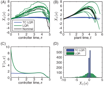
Figure 2: (A) Plots of $X_{1}(s)$ under the optimal policy and the LQR policy for $10$ realizations of $\tau_{s}$. The initial condition is $x=[0,1]^{\mathsf{T}}$. (B) The same plots under time variable $t$. The black line shows the LQR trajectory with no temporal noise. In the case of no temporal noise, the classical LQR uses high gains near $t=0$ to produces high-speed trajectories such that $Y_{1}$ approaches $0$ at final time. In this case, timing errors lead to wide variation in the final position. The optimal policy reduces the speed of the trajectory near $s=0$ order to minimize the effects of temporal noise. (C) The optimal cost $V(s,x)$ and $J(s,x;U)$ for the LQR policy are plotted for $x=[0,1]^{\mathsf{T}}$. As expected, $V(s,x)\leq J(s,x;U)$. Furthermore, as the time-horizon increases, the LQR policy depends strongly on timing information, and so temporal noise leads to higher cost as $s$ goes to $0$. (D) A histogram of the final positions, $X_{1}(S)$, for $1000$ realizations of $\tau_{s}$. The optimal controller leads to $X_{1}(S)$ being tightly distributed around $0$, while the LQR controller gives a wide spread of $X_{1}(S)$ values. The errors in the final position lead to increased cost for the LQR controller.

IV Proofs of Main Results

IV-A Proof of Theorem 1

From the definition of $X_{s}$,

$$X_{s}=X_{0}+\int_{0}^{\tau_{s}}F_{t}dt+\int_{0}^{\tau_{s}}G_{t}dW_{t}.$$ (20)

Thus, provided that (10) holds, claims 1) and 2) imply that $X_{s}$ must be an $\mathcal{F}^{\tau,W}$ semimartingale. The claims are proved as follows.

$$\mathrm{Var}\left(\int_{0}^{\tau_{s}}F_{t}dt\right)\leq\int_{0}^{\tau_{s}}\|F_{t}\|dt<\infty\textrm{ almost surely.}$$

Therefore 1) holds.

To prove 2), note that for $0\leq r\leq s$ we have

$$\mathbb{E}\left[\int_{0}^{\tau_{s}}G_{t}dW_{t}\>\vline\>\mathcal{F}^{\tau,W}_{r}\right] =\int_{0}^{\tau_{r}}G_{t}dW_{t}+\mathbb{E}\left[\int_{\tau_{r}}^{\tau_{s}}G_{t}dW_{t}\>\vline\>\mathcal{F}^{\tau,W}_{r}\right]$$

$$=\int_{0}^{\tau_{r}}G_{t}dW_{t}.$$

Furthermore,

$$\mathbb{E}\left[\left\|\int_{0}^{\tau_{s}}G_{t}dW_{t}\right\|\right]^{2}\leq\mathbb{E}\left[\left\|\int_{0}^{\tau_{s}}G_{t}dW_{t}\right\|^{2}\right]<\infty,$$ (21)

where the inequality follows from Jensen’s inequality. Thus 2) holds.

Now (10) must be proved. For more compact notation, define the processes $H_{t}$ and $Z_{t}$ as

$$H_{t}=\begin{bmatrix}F_{t}&G_{t}\end{bmatrix}\qquad Z_{t}=\begin{bmatrix}t\\ W_{t}\end{bmatrix}$$

so that $X_{s}$ may be written as

$$X_{s}=\int_{0}^{\tau_{s}}H_{t}dZ_{t}.$$

Note that $Z(\tau_{s})=[\tau_{s},W(\tau_{s})^{\mathsf{T}}]^{\mathsf{T}}$. Since $\tau_{s}$ is a subordinator, $W(\tau_{s})$ is a Lévy process on $\mathbb{R}^{d}$, with Lévy symbol

$$\eta_{W_{\tau}}(z)=-\frac{1}{2}bz^{\mathsf{T}}z+\int_{\mathbb{R}^{d}}(e^{iz^{\mathsf{T}}x}-1)\mu_{W,\tau}(dt),$$

for some Lévy measure $\mu_{W,\tau}$. (See Theorem 1.3.25 and Theorem 1.3.33, respectively, in [20].) Thus, the continuous part of $W(\tau_{s})$ is a Brownian motion with $\mathbb{E}\left[W(\tau_{s})W(\tau_{s})^{\mathsf{T}}\right]=bI$.

Define the $\tilde{Z}_{s}$ by removing the jumps from $Z(\tau_{s})$.

$$\tilde{Z}_{s}=Z(\tau_{s})-\sum_{0\leq r\leq s}\left(Z(\tau_{r})-Z(\tau_{r}^{-})\right).$$

It follows that $\tilde{Z}_{s}=[bs,\sqrt{b}\tilde{W}_{s}^{\mathsf{T}}]^{\mathsf{T}}$, where $\tilde{W}_{s}$ is the Brownian motion from the theorem statement. Thus, (10) can be equivalently written as

$$X_{s}=\int_{0}^{s}H(\tau_{r^{-}})d\tilde{Z}_{s}+\sum_{0\leq r\leq s}\int_{\tau_{r^{-}}}^{\tau_{r}}H_{s}dZ_{t}$$ (22)

Now (22) will be evaluated. If $b=0$, then $\tilde{Z}_{s}=0$ and $\tau_{s}=\sum_{0\leq r\leq s}\tau_{r}-\tau_{r^{-}}$. Thus,

$$X_{s}=\sum_{0\leq r\leq s}\int_{\tau_{r^{-}}}^{\tau_{r}}H_{s}dZ_{t},$$

so, in this case, (10) holds.

Now assume $b>0$. The cases when $\tau_{s}$ has finite rate ($\lambda((0,\infty))<\infty$) and infinite rate ($\lambda((0,\infty))=\infty$) will be treated separately.

Finite Rate. Let $r_{0}=0$ and let $r_{1},r_{2},\ldots$ be the jump times of $\tau_{s}$. With probability $1$, there exist a finite (random) integer $L$ such that $L$ jumps occur over $[0,s]$. Note that (22) may be expanded as

$$X_{s} =\int_{\tau(r_{L})}^{\tau_{s}}H_{t}dZ_{t}$$ (23)

$$+\sum_{k=0}^{L-1}\left[\int_{\tau(r_{k})}^{\tau(r_{k+1}^{-})}H_{t}dZ_{t}+\int_{\tau(r_{k+1}^{-})}^{\tau(r_{k+1})}H_{t}dZ_{t}\right]$$

Let $s_{0}^{n}\leq s_{1}^{n}\leq\cdots\leq s_{K_{n}}^{n}$ be a sequence of partitions such that

$$\begin{array}[]{lc}\lim_{n\to\infty}s_{K_{n}}^{n}=\infty&a.s.\\ \lim_{n\to\infty}\sup\{|s_{k+1}^{n}-s_{k}^{n}|:k=0,\ldots,K_{n}-1\}=0&a.s.\\ \{r_{i}:r_{i}\leq s_{K_{n}}^{n}\}\subset\{s_{0}^{n},\ldots,s_{K_{n}}^{n}\}.\end{array}$$

The last condition ensures that the jump times are contained in the partition.

Note that between jumps (i.e. $s\in[r_{k},r_{k+1})$), $\tau_{s}=bs+\tau^{d}(r_{k})$, where $\tau^{d}_{s}$ is the discontinuous part of $\tau_{s}$. Since $b>0$ follows that the sequence $\tau(s_{0}^{n}),\tau(s_{1}^{n}),\ldots$, satisfies the following properties, almost surely:

$$\begin{array}[]{l}\lim_{n\to\infty}\tau(s_{K_{n}}^{n})=\infty\\ \lim_{n\to\infty}\sup\{|\tau(s_{i+1}^{n})-\tau(s_{i}^{n})|:\exists k\>\>s.t.\>\>r_{k}\leq s_{i}^{n}<r_{k+1}\}=0\end{array}$$

Using a standard argument from stochastic integration (see Theorem II.21 of [28]), the integral from $\tau(r_{k})$ to $\tau(r_{k+1}^{-})$ may be evaluated as

$$\int_{\tau(r_{k})}^{\tau(r_{k+1}^{-})}H_{s}dZ_{t}$$

$$=\lim_{n\to\infty}\sum_{r_{k}\leq s_{i}^{n}<r_{k+1}}H(\tau(s_{i}^{n}))\left(Z(\tau(s_{i+1}))-Z(\tau(s_{i}))\right)$$

$$=\lim_{n\to\infty}\sum_{r_{k}\leq s_{i}^{n}<r_{k+1}}H(\tau(s_{i}^{n}))\left(\tilde{Z}(s_{i+1})-\tilde{Z}(s_{i})\right)$$

$$=\int_{r_{k}}^{r_{k+1}}H(\tau_{s^{-}})d\tilde{Z}_{s}.$$ (24)

The second equality uses the fact that no jumps occur over $(r_{k},r_{k+1})$. The result now follows by combining (23) and (24).

Infinite Rate. Let $\epsilon_{n}>0$ be a sequence decreasing to $0$, at a rate to be specified later. Define $\tau_{s}^{n}$ to be the process by removing all jumps of size at most $\epsilon_{n}$ from $\tau_{s}$:

$$\tau_{s}^{n}=bs+\int_{\epsilon_{n}}^{\infty}tN(s,dt).$$ (25)

Let $r_{0}^{n}=0$, and let $r_{1}^{n},r_{2}^{n},\ldots$ be the jump times of $\tau^{n}_{s}$. Let $L_{s}^{n}=\sup\{k:r_{k}^{n}\leq s\}$. With probability $1$, $L_{s}^{n}<\infty$. If $\epsilon_{n}$ are chosen as in Lemma 3 from Appendix A, then $X_{s}$ may be computed as a limit

$$X_{s}=\lim_{n\to\infty}\left[\int_{\tau(r_{L_{s}^{n}}^{n})}^{\tau_{s}}H_{t}dZ_{t}\right.$$ (26)

$$+\sum_{k=0}^{L_{s}^{n}-1}H(\tau(r_{k}^{n}))\left(Z(\tau(r_{k+1}^{n-}))-Z(\tau(r_{k}^{n}))\right)$$

$$\left.+\sum_{k=0}^{L_{s}^{n}-1}\int_{\tau(r_{k+1}^{n-})}^{\tau(r_{k+1}^{n})}H_{t}dZ_{t}\right].$$

Note that $Z(\tau(r_{k+1}^{n-}))-Z(\tau(r_{k}^{n}))$ may be expressed as

$$Z(\tau(r_{k+1}^{n-}))-Z(\tau(r_{k}^{n}))$$

$$=\tilde{Z}(r_{k+1}^{n})-\tilde{Z}(r_{k}^{n})+\sum_{\begin{subarray}{c}r_{k}^{n}<r\leq r_{k+1}^{n}\\ \Delta\tau_{r}\leq\epsilon_{n}\end{subarray}}\left(Z(\tau_{r})-Z(\tau_{r^{-}})\right).$$

Note that the terms in the summation all vanish as $\epsilon_{n}\to 0$. Furthermore, $r_{L_{s}^{n}}^{n}\uparrow s$, almost surely. Thus, (26) can be expressed as

$$X_{s} =\lim_{n\to\infty}\left[\sum_{k=0}^{L_{s}^{n}-1}H(\tau(r_{k}^{n}))\left(\tilde{Z}(r_{k+1})-\tilde{Z}(r_{k})\right)\right.$$

$$\left.+\sum_{k=0}^{L_{s}^{n}-1}\int_{\tau(r_{k+1}^{n-})}^{\tau(r_{k+1}^{n})}H_{t}dZ_{t}\right],$$

and the result now follows using Theorem II.21 of [28]. ∎

IV-B Proof of Theorem 2

Theorem 2 is a special case of finite-horizon dynamic programming for controlled Markov processes (Theorem III.8.1 of [27]), provided that the following two conditions hold for all $h\in\mathcal{D}$:

1. The backward evolution operator, defined in (12) is given by the formula in (15).

2. If

   $$\mathbb{E}\left[|h(S,X_{S})|\>|\>X_{s}=x\right]<\infty$$

   and

   $$\mathbb{E}\left[\int_{s}^{S}\left|\mathcal{A}^{U_{r}}h(r,X_{r})\right|dr\>\vline\>X_{s}=x\right]<\infty,$$

   then the Dynkin formula holds:

   $$\mathbb{E}\left[h(S,X_{S})\>\vline\>X_{s}=x\right]-h(s,x)\\ =\mathbb{E}\left[\int_{s}^{S}\mathcal{A}^{U_{r}}h(r,X_{r})dr\>\vline\>X_{s}=x\right].$$ (27)

First, using Theorem 1, a more explicit formula for $X_{s}$ is derived, and then using Itô’s formula for semimartingales, a formula for $h(s,X_{s})$ is given. Using the formula for $h(s,X_{s})$, equations (12) and (27) are then proved.

Note that $Y(\tau_{r^{-}})=X_{r^{-}}$ and for all $t\in[\tau_{r^{-}},\tau_{r}]$, $\zeta_{t}=r$. Therefore

$$F(\zeta(\tau_{r^{-}}),Y_{\tau_{r^{-}}},U(\zeta(\tau_{r^{-}})))=F(r,X_{r^{-}},U_{r})$$

$$F(\zeta_{t},Y_{t},U(\zeta_{t}))=F(r,Y_{t},U_{r})\qquad\textrm{for all}\qquad t\in[\tau_{r^{-}},\tau_{r}].$$

The expressions for $G$ are similar. Thus, Theorem 1 implies that $X_{s}$ is given by

$$X_{s}=X_{0}+b\int_{0}^{s}F(r,X_{r^{-}},U_{r})dr+\sqrt{b}\int_{0}^{s}G(r,X_{r^{-}},U_{r})d\tilde{W}_{r}\\ +\sum_{0\leq r\leq s}\left(\int_{\tau_{r^{-}}}^{\tau_{r}}F(r,Y_{t},U_{r})dt+\int_{\tau_{r^{-}}}^{\tau_{r}}G(r,Y_{t},U_{r})dW_{t}\right).$$ (28)

Now a formula for $h(s,X_{s})$ will be derived. Note that for any càglàd, $\mathcal{F}^{\tau,W}$-adapted process, $Z_{s}$, the stochastic integral with respect to $X_{s}$ is given by

$$\int_{0}^{s}Z_{r}dX_{r}=\int_{0}^{s}Z_{r}bF(r,X_{r^{-}},U_{r})dr\\ +\int_{0}^{s}Z_{r}\sqrt{b}G(r,X_{r^{-}},U_{r})dW_{r}+\sum_{0\leq r\leq s}Z_{r}(X_{r}-X_{r^{-}}).$$

Furthermore, the continuous part of the quadratic variation is given by

$$[X,X]_{s}^{c}=\int_{0}^{s}\frac{1}{2}bG(r,X_{r^{-}},U_{r})G(r,X_{r^{-}},U_{r})^{\mathsf{T}}dr.$$

Thus Itô’s formula for semimartingales (see [28]) implies that $h(s,X_{s})$ is given by

$$h(s,X_{s})=h(0,X_{0})\\ +\int_{0}^{s}\left(\frac{\partial h(r,X_{r^{-}})}{\partial r}+b\frac{\partial h(r,X_{r^{-}})}{\partial x}F(r,X_{r^{-}},U_{r})\right)dr\\ +\int_{0}^{s}\frac{1}{2}b\mathrm{Tr}\left(G(r,X_{r^{-}},U_{r})^{\mathsf{T}}\frac{\partial^{2}h(r,X_{r^{-}})}{\partial x^{2}}G(r,X_{r^{-}},U_{r})\right)dr\\ +\int_{0}^{s}\sqrt{b}\frac{\partial h(r,X_{r^{-}})}{\partial x}G(r,X_{r^{-}},U_{r})d\tilde{W}_{r}\\ +\sum_{0\leq r\leq s}\left(h(r,X_{r})-h(r,X_{r^{-}})\right).$$ (29)

Now (12) will be derived from (29). Assume that $X_{s}=x$ and $U_{r}=u$ for $r\in[s,s+h]$. Then (29) implies that

$$\mathbb{E}[h(s+h,X_{s+h})]=h(s,x)\\ +\mathbb{E}\left[\int_{s}^{s+h}\left(\frac{\partial h(r,X_{r^{-}})}{\partial r}+b\frac{\partial h(r,X_{r^{-}})}{\partial x}F(r,X_{r^{-}},u)\right)dr\right]\\ +\mathbb{E}\left[\frac{1}{2}b\mathrm{Tr}\left(G(r,X_{r^{-}},u)^{\mathsf{T}}\frac{\partial^{2}h(r,X_{r^{-}})}{\partial x^{2}}G(r,X_{r^{-}},u)\right)dr\right]\\ +\mathbb{E}\left[\sum_{s<r\leq s+h}\left(h(r,X_{r})-h(r,X_{r^{-}})\right)\right].$$ (30)

If $r>s$, the Brownian motions $W_{t}$ for $t\in[\tau_{r^{-}},\tau_{r}]$ and $\hat{W}_{t}$ for $t\in[0,\Delta\tau_{r}]$ are identically distributed and independent of $\mathcal{F}_{s}^{\tau,W}$. Therefore, using (13), and given that $X_{s}=x$ and $U_{r}=u$, the expectations of the jump terms may be written as

$$\mathbb{E}\left[h(r,X_{r})-h(r,X_{r^{-}})\right]=$$

$$\mathbb{E}\left[\mathbb{E}_{\hat{W}}\left[h\left(r,Y_{r,\Delta\tau_{r}}^{X_{r^{-}}u}\right)\right]-h(r,X_{r^{-}})\right].$$

Thus, the term at the bottom of (30) may be evaluated as a Poisson integral:

$$\mathbb{E}\left[\sum_{s<r\leq s+h}\left(h(r,X_{r})-h(r,X_{r^{-}})\right)\right]$$

$$=\mathbb{E}\left[\int_{s}^{s+h}\int_{0}^{\infty}\left(\mathbb{E}_{\hat{W}}\left[h\left(r,Y_{rt}^{X_{r^{-}}u}\right)\right]-h(r,X_{r^{-}})\right)N(dr,dt)\right]$$

$$=\mathbb{E}_{W}\left[\int_{s}^{s+h}\int_{0}^{\infty}\left(\mathbb{E}_{\hat{W}}\left[h\left(r,Y_{rt}^{X_{r^{-}}u}\right)\right]-h(r,X_{r^{-}})\right)\lambda(dt)dr\right]$$

where the second is equation is justified by Fubini’s theorem and (14).

By evaluating the limit on the right side of (12), the formula in (15) is recovered.

Turning to (27), since $X_{s}$ is $\mathcal{F}_{s}^{\tau,W}$ measurable, it suffices to prove that

$$\mathbb{E}\left[h(S,X_{S})-h(s,X_{s})-\int_{s}^{S}\mathcal{A}^{U_{s}}h(r,X_{r})dr\>\vline\>\mathcal{F}_{s}^{\tau,W}\right]=0.$$

Since $X_{r}(\omega)=X_{r^{-}}(\omega)$ for almost all $(r,\omega)\in[s,S]\times\Omega$, it follows that

$$\mathbb{E}\left[\int_{s}^{S}\mathcal{A}^{U_{s}}h(r,X_{r})dr\>\vline\>\mathcal{F}_{s}^{\tau,W}\right]=$$

$$\mathbb{E}\left[\int_{s}^{S}\mathcal{A}^{U_{s}}h(r,X_{r^{-}})dr\>\vline\>\mathcal{F}_{s}^{\tau,W}\right].$$

Combining (15) and (29) and, for brevity, omitting $\mathcal{F}_{s}^{\tau,W}$ from the expectations, implies that

$$\mathbb{E}\left[h(S,X_{S})-h(s,X_{s})-\int_{s}^{S}\mathcal{A}^{U_{r}}h(r,X_{r^{-}})dr\right]=\\ \mathbb{E}\left[\sum_{s<r\leq S}\left(h(r,X_{r})-h(r,X_{r^{-}})\right)\right]-\\ \mathbb{E}\left[\int_{s}^{S}\int_{0}^{\infty}\left(\mathbb{E}_{\hat{W}}[h(r,Y_{t}^{X_{r^{-}}U_{r}})]-h(r,X_{r^{-}})\right)\lambda(dt)dr\right],$$ (31)

As in the proof of (12), the two terms at the bottom of (31) are equal in expectation. Thus (27) holds and the proof is complete. ∎

IV-C Proof of Theorem 3

Assume $V(s,x)=x^{\mathsf{T}}P_{s}x+h_{s}$. Applying the backward evolution operator corresponding to (18) to $V(s,x)$ results in

$$\mathcal{A}^{u}V(s,x)=x^{\mathsf{T}}\dot{P}_{s}x+\dot{h}_{s}+bx^{\mathsf{T}}(A^{\mathsf{T}}P_{s}+P_{s}A)x+2bx^{\mathsf{T}}P_{s}Bu$$ (32)

$$+b\mathrm{Tr}\left(P_{s}MM^{\mathsf{T}}\right)+\int_{0}^{\infty}\left(\mathbb{E}_{\hat{W}}\left[{Y_{t}^{xu}}^{\mathsf{T}}P_{s}Y_{t}^{xu}\right]-x^{\mathsf{T}}P_{s}x\right)\lambda(dt).$$

Note that $\mathbb{E}_{\hat{W}}\left[Y_{t}^{xu}{Y_{t}^{xu}}^{\mathsf{T}}\right]$ may be evaluated at

$$\mathbb{E}_{\hat{W}}\left[Y_{t}^{xu}{Y_{t}^{xu}}^{\mathsf{T}}\right]=y_{t}^{xu}{y_{t}^{xu}}^{\mathsf{T}}+\Sigma_{t},$$

where $y_{t}^{xu}$ is the mean of $Y_{t}^{xu}$ and $\Sigma_{t}$ is the covariance. A standard argument in linear stochastic differential equations shows that the mean and covariance are given by

$$y_{t}^{xu} =e^{At}x+\int_{0}^{t}e^{Ar}drBu,$$

$$\Sigma_{t} =\int_{0}^{t}e^{Ar}MM^{\mathsf{T}}e^{A^{\mathsf{T}}r}dr.$$

Thus, the integral in (32) may be written as

$$\int_{0}^{\infty}\left(\mathbb{E}_{\hat{W}}\left[{Y_{t}^{xu}}^{\mathsf{T}}P_{s}Y_{t}^{xu}\right]-x^{\mathsf{T}}P_{s}x\right)\lambda(dt)=$$ (33)

$$\int_{0}^{\infty}\begin{bmatrix}x\\ u\end{bmatrix}^{\mathsf{T}}\begin{bmatrix}\hat{F}(t,P_{s})&\hat{G}(t,P_{s})B\\ B^{\mathsf{T}}\hat{G}(t,P_{s})^{\mathsf{T}}&B^{\mathsf{T}}\hat{H}(t,P_{s})B\end{bmatrix}\begin{bmatrix}x\\ u\end{bmatrix}\lambda(dt)$$

$$+\int_{0}^{\infty}\int_{0}^{t}\mathrm{Tr}\left(P_{s}e^{Ar}MM^{\mathsf{T}}e^{A^{\mathsf{T}}r}\right)dr\lambda(dt),$$

where the matrices $\hat{F}$, $\hat{G}$, and $\hat{H}$ are defined by

$$\hat{F}(t,P) =e^{A^{\mathsf{T}}t}Pe^{At}-P,$$

$$\ \hat{G}(t,P) =e^{A^{\mathsf{T}}t}P\int_{0}^{t}e^{A\rho}d\rho,$$

$$\hat{H}(t,P) =\int_{0}^{t}e^{A^{\mathsf{T}}r}drP\int_{0}^{t}e^{A\rho}d\rho.$$

Combining (32) and (33), and using the linear operators from Lemma 2 gives

$$\mathcal{A}^{u}V(s,x)=\begin{bmatrix}x\\ u\end{bmatrix}^{\mathsf{T}}\begin{bmatrix}\dot{P}_{s}+F(P_{s})&G(P_{s})B\\ B^{\mathsf{T}}G(P_{s})&B^{\mathsf{T}}H(P_{s})B\end{bmatrix}\begin{bmatrix}x\\ u\end{bmatrix}+\dot{h}_{s}+g(P_{s}).$$

Therefore, adding the cost gives

$$x^{\mathsf{T}}Qx+u^{\mathsf{T}}Ru+\mathcal{A}^{u}V(s,x)=\dot{h}_{s}+g(P_{s})$$

$$+\begin{bmatrix}x\\ u\end{bmatrix}^{\mathsf{T}}\begin{bmatrix}Q+\dot{P}_{s}+F(P_{s})&G(P_{s})B\\ B^{\mathsf{T}}G(P_{s})&R+B^{\mathsf{T}}H(P_{s})B\end{bmatrix}\begin{bmatrix}x\\ u\end{bmatrix}.$$

The result now follows from quadratic minimization. ∎

V Discussion

The work in this paper lays a theoretical foundation for future research on biological motor control [29, 30], finance [31], and multi-agent control [32, 33] in context that the controller is uncertain about the time of the plant. To reason about these problems, theoretical extensions will include time estimation from sensory data, optimal control control with different time horizons, and control with multiple noisy clocks.

Time Estimation

This paper focuses on state feedback problems, and the optimal solution from dynamic programming only depends on the value of the current state. For other problems, an explicit estimate of time could be valuable. In option pricing, inferences about the “business time” can be used to estimate the volatility of stock prices [34]. To perceive time, humans appear to integrate sensory cues about the passage of time in a Bayesian manner [35]; humans also appear to incorporate sensory information about the timing of events to improve state estimation [36].

In order to obtain a well-posed estimation problem, plant time ($\tau_{s}$) can be modeled as an unmeasured state. Particle filtering techniques to estimate $\tau_{s}$ are currently being developed.

In dance and music performance, movements are coordinated with an estimate of time. The work in this paper will be combined with filtering methods to model experimental data on timed movements.

Variations on the Horizon

This paper studies a controller horizon $[0,S]$, which is an interval of time with respect to the clock measured by the controller. For portfolio optimization, in which the controller measures calendar time, such a horizon is sensible. In human movements, however, different tasks call for different time horizons. When reaching to an object, a natural horizon would be the stopping time describing when the object is touched. For rhythmic movements coordinated with external stimuli such as a metronome, a horizon over real time might be sensible.

Multiple Clocks

In this paper, it is assumed that the plant dynamics evolve according to one clock, while the controller can measure a different clock. If the plant consists of numerous subsystems, then each could potentially evolve according to a different clock. This scenario arises in portfolio problems, in which the goal is to allocate wealth between a bank process which accrues interest at known, fixed rate and a stock process that evolves in a variable rate market [22]. Here, the bank process may be interpreted as evolving with respect to a perfect clock, while the stock process may be viewed as evolving with respect to a noisy clock. In engineering applications, such as mobile sensor networks, multiple autonomous agents with their own clocks solve cooperative control problems. Currently, problems arising from drift between clocks are mitigated by using expensive clocks and time synchronization protocols. The work in this paper will be extended to reduce the need for precision timing and synchronization.

VI Conclusion

This paper gives basic results on control with uncertainty in time. The technical backbone of the paper is Theorem 1 which expresses the original plant dynamics in terms of the controller’s clock index. Using the new representation, the system becomes a controlled Markov process, and thus existing dynamic programming theory can be applied. Given the dynamic programming equations, time changed versions of linear quadratic control and a nonlinear portfolio problem problem are solved explicitly.

Appendix A A Technical Lemma for Theorem 1

Lemma 3

Let $\tau_{s}$ be an infinite rate subordinator. Let $r_{0}^{n}=0$ and let $r_{1}^{n}\leq r_{2}^{n}\leq\cdots$ be the jump times of $\tau_{s}^{n}$, from (25). There is a sequence $S_{n}\to\infty$ and a sequence $\epsilon_{n}\downarrow 0$ such that the following limits hold, almost surely

$$\lim_{n\to\infty}\sup\{r_{i}^{n}:r_{i}^{n}\leq S_{n}\} =\infty$$ (34)

$$\lim_{n\to\infty}\sup\{\tau_{r_{i}^{n}}:r_{i}^{n}\leq S_{n}\} =\infty$$ (35)

$$\lim_{n\to\infty}\sup\{r_{i+1}^{n}-r_{i}^{n}:r_{i}^{n}\leq S_{n}\} =0$$ (36)

$$\lim_{n\to\infty}\sup\{\tau_{r_{i+1}^{n-}}-\tau_{r_{i}^{n}}:r_{i}^{n}\leq S_{n}\} =0.$$ (37)

Proof:

First it will be shown that for any sequence $S_{n}>0$, a sequence $\epsilon_{n}\downarrow 0$ can be chosen such that (36) and (37) hold. Then it will be shown how to choose $S_{n}$ so that (34) and (35) hold.

Consider (36). Using Borel’s lemma, it is sufficient to prove that for some constant $R>0$, and $\epsilon_{n}$ sufficiently small,

$$\mathbb{P}\left(\sup_{r_{i}^{n}\leq S_{n}}|r_{i+1}^{n}-r_{i}^{n}|\geq\frac{1}{2^{n}}\right)<\frac{R}{2^{n}}.$$ (38)

For ease of notation, the superscripts on $r_{i}^{n}$ and the subscripts on $\epsilon_{n}$ and $S_{n}$ will be dropped.

With probability $1$, $\tau_{s}^{n}$ has only a finite number of jumps over $[0,S]$, so let $K=\max\{i:r_{i}\leq S\}$.

Consider (38). Define the function $g(\epsilon)$ by

$$g(\epsilon)=\int_{\epsilon}^{\infty}\lambda(dt).$$

Note that the differences are $r_{i+1}-r_{i}$ are exponential random variables with rate parameter $g(\epsilon)$. Thus, the event that $r_{i+1}-r_{i}\geq 1/2^{n}$ is a Bernoulli random variable with probability $p(\epsilon)$ given by

$$p(\epsilon)=\mathbb{P}\left(r_{i+1}-r_{i}\geq\frac{1}{2^{n}}\right)=g(\epsilon)\int_{1/2^{n}}^{\infty}e^{-g(\epsilon)x}dx=e^{-g(\epsilon)/2^{n}}.$$

Let $J$ be the geometric random variable defined by

$$J=\min\left\{i:r_{i+1}-r_{i}\geq\frac{1}{2^{n}}\right\}$$

Then the probability of $J$ is given by

$$\mathbb{P}(J=k)=(1-p(\epsilon))^{k}p(\epsilon).$$

Using the definition of $K$ and $J$, the probability in (38) may be written as

$$\mathbb{P}\left(\sup_{r_{i}\leq S}|r_{i+1}-r_{i}|\geq\frac{1}{2^{n}}\right)=\mathbb{P}(J\leq K).$$

Furthermore, given any constant $M>0$,

$$\mathbb{P}(J\leq K)\leq\mathbb{P}(J\leq M)+\mathbb{P}(M\leq K).$$ (39)

Thus, (38) may be bounded by bounding the terms on the right of (39) separately.

Now $\mathbb{P}(M\leq K)$ will be bounded. Note that $K$ is a Poisson random variable with parameter $Sg(\epsilon)$. Markov’s inequality thus shows that

$$\mathbb{P}(M\leq K)\leq\frac{1}{M}\mathbb{E}[K]=\frac{Sg(\epsilon)}{M}$$ (40)

The term $\mathbb{P}(J\leq M)$ can be computed exactly as

$$\mathbb{P}(J\leq M)=p(\epsilon)\sum_{k=0}^{M}(1-p(\epsilon))^{k}=1-(1-p(\epsilon))^{M+1}.$$

Thus, (38) will hold if $M$ can be chosen such that

$$Sg(\epsilon)/M<1/2^{n}\quad\textrm{and}\quad 1-(1-p(\epsilon))^{M+1}<1/2^{n}.$$ (41)

Rearranging terms, (41) is equivalent to

$$2^{n}Sg(\epsilon)<M<\frac{\log\left(1-\frac{1}{2^{n}}\right)}{\log(1-p(\epsilon))}-1.$$

Therefore, a suitable constant $M$ exists if

$$\left(2^{n}Sg(\epsilon)+1\right)\log(1-p(\epsilon))>\log\left(1-\frac{1}{2^{n}}\right).$$ (42)

It will be shown that (42) holds provided that $\epsilon$ is sufficiently small. Since $\tau_{s}$ has infinite rate, $\lim_{\epsilon\to 0}g(\epsilon)=\infty$. Thus, the limit of the left side of (42) may be evaluated by L’Hôspital’s rule:

$$\lim_{\epsilon\to 0}\left(2^{n}Sg(\epsilon)+1\right)\log(1-p(\epsilon)) =\lim_{g\to\infty}\frac{\log(1-e^{-g/2^{n}})}{\left(2^{n}Sg+1\right)^{-1}}$$

$$=\lim_{g\to\infty}\frac{\frac{e^{-g/2^{n}}/2^{n}}{1-e^{-g/2^{n}}}}{-2^{n}S\left(2^{n}Sg+1\right)^{-2}}$$

$$=-\frac{1}{4^{n}S}\lim_{g\to\infty}\frac{\left(2^{n}Sg+1\right)^{2}}{e^{g/2^{n}}-1}$$

$$=0.$$

Thus, when $\epsilon$ is sufficiently small, (38) must hold.

Now consider (37). Note that $\tau_{r_{i+1}^{n-}}-\tau_{r_{i}^{n}}$ can be expressed as

$$\tau_{r_{i+1}^{n-}}-\tau_{r_{i}^{n}}=b(r_{i+1}^{n}-r_{i}^{n})+\sum_{\begin{subarray}{c}r_{i}^{n}<u\leq r_{i+1}^{n}\\ \Delta\tau_{u}\leq\epsilon_{n}\end{subarray}}\Delta\tau_{u}$$

Thus

$$\sup_{r_{i}^{n}\leq S_{n}}|\tau_{r_{i+1}^{n-}}-\tau_{r_{i}^{n}}|\leq b\sup_{r_{i}^{n}\leq S_{n}}|r_{i+1}^{n}-r_{i}^{n}|+\sup_{r_{i}\leq S_{n}}\sum_{\begin{subarray}{c}r_{i}^{n}<u\leq r_{i+1}^{n}\\ \Delta\tau_{u}\leq\epsilon_{n}\end{subarray}}\Delta\tau_{u}$$

It has already been shown that the first term on the right converges to $0$ almost surely. Thus to prove (37), it suffices to prove that

$$\lim_{n\to\infty}\sup_{r_{i}^{n}\leq S_{n}}\sum_{\begin{subarray}{c}r_{i}^{n}<u\leq r_{i+1}^{n}\\ \Delta\tau_{u}\leq\epsilon_{n}\end{subarray}}\Delta\tau_{u}=0,$$ (43)

almost surely, when $\epsilon_{n}\downarrow 0$ sufficiently quickly. Again, by Borel’s lemma, (43) will follow if $\epsilon_{n}$ is chosen such that

$$\mathbb{P}\left(\sup_{r_{i}^{n}\leq S_{n}}\sum_{\begin{subarray}{c}r_{i}^{n}<u\leq r_{i+1}^{n}\\ \Delta\tau_{u}\leq\epsilon_{n}\end{subarray}}\Delta\tau_{u}\geq\frac{1}{2^{n}}\right)<\frac{R}{2^{n}},$$ (44)

for some $R>0$.

As before, suppress the superscripts on $r_{i}^{n}$ and the subscripts on $\epsilon_{n}$ and $S_{n}$. Recall that $r_{i+1}-r_{i}$ are exponential random variables with rate parameter $g(\epsilon)$. Furthermore, the jump times of $\tau_{s}^{n}$ are independent of the small-jumps process

$$\tau_{s}-\tau_{s}^{n}=\sum_{\begin{subarray}{c}0\leq r\leq s\\ \Delta\tau_{r}\leq\epsilon\end{subarray}}\Delta\tau_{r}.$$

Define $h(\epsilon)$ by

$$h(\epsilon)=\int_{0}^{\epsilon}t\lambda(dt).$$

Let $q(\epsilon)$ be the probability that $\sum_{\begin{subarray}{c}r_{i}^{n}<u\leq r_{i+1}^{n}\\ \Delta\tau_{u}\leq\epsilon_{n}\end{subarray}}\Delta\tau_{u}\geq\frac{1}{2^{n}}$. Define $\hat{q}(\epsilon)$ as the upper bound on $q(\epsilon)$ given by Markov’s inequality:

$$q(\epsilon)=\mathbb{P}\left(\sum_{\begin{subarray}{c}r_{i}^{n}<u\leq r_{i+1}^{n}\\ \Delta\tau_{u}\leq\epsilon_{n}\end{subarray}}\Delta\tau_{u}\geq\frac{1}{2^{n}}\right)\leq$$ (45)

$$2^{n}\mathbb{E}\left[\sum_{\begin{subarray}{c}r_{i}^{n}<u\leq r_{i+1}^{n}\\ \Delta\tau_{u}\leq\epsilon_{n}\end{subarray}}\Delta\tau_{u}\right]=2^{n}\mathbb{E}\left[\int_{r_{i}}^{r_{i+1}}\int_{0}^{\epsilon}tN(dr,dt)\right]=\frac{2^{n}h(\epsilon)}{g(\epsilon)}.$$

As in the proof of (38), the bound in (44) will be recast as a more tractable inequality.

Let $L$ be the geometric random variable defined by

$$L=\min\left\{i:\sum_{\begin{subarray}{c}r_{i}<u\leq r_{i+1}\\ \Delta\tau_{u}\leq\epsilon\end{subarray}}\Delta\tau_{u}\geq\frac{1}{2^{n}}\right\}.$$

So $L$ has probability given by $\mathbb{P}(L=k)=(1-q(\epsilon))^{k}q(\epsilon)$. As in the proof of (38), for any constant $M>0$,

$$\mathbb{P}\left(\sup_{r_{i}\leq S}\sum_{\begin{subarray}{c}r_{i}<u\leq r_{i+1}\\ \Delta\tau_{u}\leq\epsilon\end{subarray}}\Delta\tau_{u}\geq\frac{1}{2^{n}}\right)=$$

$$\mathbb{P}(L\leq K)\leq\mathbb{P}(L\leq M)+\mathbb{P}(M\leq K).$$

The first term on the right can be bounded as

$$\mathbb{P}(L\leq M)=1-(1-q(\epsilon))^{M+1}\leq 1-(1-\hat{q}(\epsilon))^{M+1}.$$

Furthermore, as in the proof of (38), if

$$\left(2^{n}Sg(\epsilon)+1\right)\log(1-\hat{q}(\epsilon))<\log\left(1-\frac{1}{2^{n}}\right),$$ (46)

the constant $M$ can be chosen such that

$$\mathbb{P}(L\leq M)+\mathbb{P}(M\leq K)\leq\frac{2}{2^{n}}.$$

Thus, if (46) holds, then so does (44). Note that $\hat{q}(\epsilon)\to 0$ as $\epsilon\to 0$, and thus $\log(1-\hat{q}(\epsilon))\to 0$ as well. Thus, for $\eqref{qBound}$ to hold for sufficiently small $\epsilon$, it suffices to show that $g(\epsilon)\log(1-\hat{q}(\epsilon))\to 0$ as $\epsilon\to 0$.

Using the power series expansion of $\log(1-\hat{q}(\epsilon))$ implies that

$$|g(\epsilon)\log(1-\hat{q}(\epsilon))|=g(\epsilon)\sum_{k=1}^{\infty}\frac{\hat{q}(\epsilon)^{k}}{k}=g(\epsilon)\sum_{k=1}^{\infty}\frac{2^{nk}h(\epsilon)^{k}}{g(\epsilon)^{k}k}$$

$$=2^{n}h(\epsilon)\sum_{k=0}^{\infty}\frac{\hat{q}(\epsilon)^{k}}{k+1}\leq 2^{n}h(\epsilon)\sum_{k=0}^{\infty}\hat{q}(\epsilon)^{k}=\frac{2^{n}h(\epsilon)}{1-\hat{q}(\epsilon)}.$$

Now $\lim_{\epsilon\to 0}h(\epsilon)=0$ implies that $\lim_{\epsilon\to 0}g(\epsilon)\log(1-\hat{q}(\epsilon))=0$. Therefore (46) holds for sufficiently small $\epsilon$ and the proof is complete.

Now (34) and (35) will be proved. As long as $S_{n}\to\infty$, the limit in (34) is immediate from (36) since

$$S_{n}-\sup\{r_{i}^{n}:r_{i}^{n}\leq S_{n}\}\leq\sup\{r_{i+1}^{n}-r_{i}^{n}:r_{i}^{n}\leq S_{n}\}.$$

Now (35) will be proved. If $b>0$, then (35) follows for any sequence with $S_{n}\to\infty$. Thus, assume that $b=0$. Let $K_{n}=\max\{i:r_{i}^{n}\leq S_{n}\}$ and assume that $\epsilon_{n-1}$ is fixed. The sequence in (35) may be lower-bounded as

$$\sup\{\tau_{r_{i}^{n}}^{n}:r_{i}^{n}\leq S_{n}\}=\tau_{r_{K_{n}}^{n}}\geq\tau_{r_{K_{n}}^{n}}^{n}=\tau_{S_{n}}^{n}$$

$$\geq\tau_{S_{n}}^{n-1}\geq\epsilon_{n-1}N(S_{n},(\epsilon_{n-1},\infty)).$$

The random measure term on the right is a Poisson process with rate $g(\epsilon_{n-1})$. Thus

$$\mathbb{P}\left(\sup\{\tau_{r_{i}^{n}}^{n}:r_{i}^{n}\leq S_{n}\}<n\right)\leq\mathbb{P}\left(\epsilon_{n-1}N(S_{n},(\epsilon_{n-1},\infty))<n\right)$$

Therefore, Borel’s lemma implies that it is sufficient to prove

$$\mathbb{P}\left(\epsilon_{n-1}N(S_{n},(\epsilon_{n-1},\infty))<n\right)<\frac{1}{2^{n}}.$$ (47)

The probability may be computed explicitly as

$$\mathbb{P}\left(\epsilon_{n-1}N(S_{n},(\epsilon_{n-1},\infty))<n\right)=$$

$$e^{-S_{n}g(\epsilon_{n-1})}\sum_{0\leq k<\frac{n}{\epsilon_{n-1}}}\frac{(S_{n}g(\epsilon_{n-1}))^{k}}{k}.$$

So, for fixed $\epsilon_{n-1}$, $S_{n}$ may be chosen sufficiently large so that (47) holds, and the proof is complete.      

Appendix B Proof of Lemma 1

First note that $\beta$ is analytic at $z$ if $\int_{0}^{\infty}(e^{zt}-1)\lambda(dt)$ is. Furthermore, by the Lévy-Itô decomposition,

$$\mathbb{E}[e^{z\tau_{s}}]=e^{zbs}\mathbb{E}\left[\exp\left(z\int_{0}^{\infty}tN(s,dt)\right)\right].$$

Thus, it suffices to prove the theorem for the case that $b=0$.

Consider $z\in\mathrm{dom}(\beta)$, and let $r=\mathrm{Re}\>z$. It will be shown that $\beta$ is analytic at $z$. Take any $\hat{r}\in(r,r_{\max})$ and any $y\in\mathbb{C}$ such that $|y-z|<\hat{r}-r$. Provided that the sum of integrals below converges absolutely, $\beta(y)$ can be derived from the power series expansion around $z$:

$$\int_{0}^{\infty}\left(e^{zt}-1\right)\lambda(dt)+\sum_{k=1}^{\infty}\frac{1}{k!}(y-z)^{k}\int_{0}^{\infty}t^{k}e^{zt}\lambda(dt)$$

$$=\int_{0}^{\infty}\left(e^{zt}-1\right)\lambda(dt)+\int_{0}^{\infty}\left(e^{(y-z)t}-1\right)e^{zt}\lambda(dt)$$

$$=\beta(y).$$ (48)

Note that the form of the derivatives is immediate from the series expansion.

For absolute convergence, note that

$$\int_{0}^{\infty}\left|e^{zt}-1\right|\lambda(dt)+\sum_{k=1}^{\infty}\frac{1}{k!}|y-z|^{k}\int_{0}^{\infty}\left|t^{k}e^{zt}\right|\lambda(dt)=$$ (49)

$$\int_{0}^{\infty}\left|e^{zt}-1\right|\lambda(dt)+\sum_{k=1}^{\infty}\frac{1}{k!}|y-z|^{k}\int_{0}^{\infty}t^{k}e^{rt}\lambda(dt).$$

The first term on the right is seen to be finite as follows. If $t\in[0,1]$, then

$$\left|e^{zt}-1\right|=\left|\sum_{k=1}^{\infty}\frac{(zt)^{k}}{k!}\right|\leq t\sum_{k=1}^{\infty}\frac{|z|^{k}}{k!}=t\left(e^{|z|}-1\right).$$

On the other hand, the triangle inequality implies that

$$\left|e^{zt}-1\right|\leq\left|e^{zt}\right|+1=e^{rt}+1.$$

Therefore, the first integral on the right of (49) is bounded as

$$\int_{0}^{\infty}\left|e^{zt}-1\right|\lambda(dt)$$ (50)

$$\leq\left(e^{|z|}-1\right)\int_{0}^{1}t\lambda(dt)+\int_{1}^{\infty}\left(e^{rt}+1\right)\lambda(dt)<\infty,$$

where the last inequality follows since $r<r_{\max}$.

Now the integral in the sum on the right of (49) will be bounded. First note that the integrand is bounded as

$$t^{k}e^{rt}=t^{k}e^{-(\hat{r}-r)t}e^{\hat{r}t}\leq\left(\frac{k}{e(\hat{r}-r)}\right)^{k}e^{\hat{r}t},$$ (51)

where the inequality follows from maximizing $te^{-(\hat{r}-r)t}$. Thus, the integral is bounded as

$$\int_{0}^{\infty}t^{k}e^{rt}\lambda(dt)\leq e^{r}\int_{0}^{1}t\lambda(dt)+\left(\frac{k}{e(\hat{r}-r)}\right)^{k}\int_{1}^{\infty}e^{\hat{r}t}\lambda(dt)$$ (52)

Thus, to prove that the sum on the right of (49) converges, it suffices to prove that

$$\sum_{k=1}^{\infty}\frac{|y-z|^{k}}{k!}\left(\frac{k}{e(\hat{r}-r)}\right)^{k}<\infty$$

Now, the Stirling approximation bound, $k!\geq\sqrt{2\pi k}\left(\frac{k}{e}\right)^{k}$, shows that

$$\frac{1}{k!}\left(\frac{k}{e(\hat{r}-r)}\right)^{k}\leq\frac{1}{\sqrt{2\pi k}(\hat{r}-r)^{k}}\leq\frac{1}{(\hat{r}-r)^{k}}.$$

Since $|y-z|<\hat{r}-r$, the bound follows as

$$\sum_{k=1}^{\infty}\frac{|y-z|^{k}}{k!}\left(\frac{k}{e(\hat{r}-r)}\right)^{k}\leq\sum_{k=1}^{\infty}\left(\frac{|y-z|}{\hat{r}-r}\right)^{k}<\infty.$$

Thus, the power series expansion, (48) holds, and $\beta$ is analytic at $z$.

Now (4) will be proved. The proof is similar to the proof of Theorem 2.3.8 in [20].

First, the function $t$ will be approximated by step functions over $(0,\infty)$. The construction is similar to the approach in the proof of Theorem 1.17 in [37]. Consider a sequence $\gamma_{n}\downarrow 0$ at a rate to be specified later. Let $k_{n}(t)$ be the unique integer such that $k\gamma_{n}\leq t<(k+1)\gamma_{n}$. Define the function $\varphi_{n}(t)$ by

$$\varphi_{n}(t)=\left\{\begin{matrix}k_{n}(t)\gamma_{n}&\qquad t\in(0,n)\\ n&\qquad t\geq n.\end{matrix}\right.$$

Then $\varphi_{n}(t)$ is a simple function such that $\varphi_{n}(t)=0$ for $t\in(0,\gamma_{n})$, $t-\gamma_{n}<\varphi_{n}(t)\leq t$ for $t\in[\gamma_{n},n]$, and $\varphi_{n}(t)\leq t$ for $t>0$. The formula, (4), is a consequence of the following chain of equalities

$$\mathbb{E}\left[\exp\left(z\int_{0}^{\infty}tN(s,dt)\right)\right]$$

$$=\lim_{n\to\infty}\mathbb{E}\left[\exp\left(z\int_{0}^{\infty}\varphi_{n}(t)N(s,dt)\right)\right]$$ (53)

$$=\lim_{n\to\infty}\exp\left(s\int_{0}^{\infty}\left(e^{z\varphi_{n}(t)}-1\right)\lambda(dt)\right)$$ (54)

$$=\exp\left(s\int_{0}^{\infty}\left(e^{zt}-1\right)\lambda(dt)\right).$$ (55)

The first equation is the most challenging, and will be handled last. To prove (54), note that $z\varphi_{n}(t)$ is a simple function. Thus, there are constants $c_{i}\in\mathbb{C}$ and disjoint $\lambda$-measurable sets, $A_{i}$, such that

$$z\varphi_{n}(t)=\sum_{i=1}^{q}c_{i}\mathbf{1}_{A_{i}}(t).$$

Since $\varphi_{n}(t)=0$ over $(0,\gamma_{n})$, it follows that $0$ is not in the closure of any $A_{i}$. Thus, the integral on the right of (53) may be written as

$$\int_{0}^{\infty}z\varphi_{n}(t)N(s,dt)=\sum_{i=1}^{q}c_{i}N(s,A_{i}),$$

where $N(s,A_{i})$ are independent Poisson processes with rate $\lambda(A_{i})$. Thus, the expectation on the right of (53) may be calculated as

$$\mathbb{E}\left[\exp\left(z\int_{0}^{\infty}\varphi_{n}(t)N(s,dt)\right)\right]$$

$$=\prod_{i=1}^{q}\mathbb{E}\left[\exp(c_{i}N(s,A_{i}))\right]$$

$$=\prod_{i=1}^{q}\exp(-s\lambda(A_{i}))\sum_{k=0}^{\infty}\frac{(s\lambda(A_{i}))^{k}}{k!}e^{c_{i}k}$$

$$=\prod_{i=1}^{q}\exp\left(s\lambda(A_{i})\left(e^{c_{i}}-1\right)\right)$$

$$=\exp\left(s\sum_{i=1}^{q}\left(e^{c_{i}}-1\right)\lambda(A_{i})\right)$$

$$=\exp\left(s\int_{0}^{\infty}\left(e^{z\varphi_{n}(t)}-1\right)\lambda(dt)\right).$$

Thus, (54) holds.

To prove (55), note that (50) implies that $\left|e^{z\varphi_{n}(t)}-1\right|$ is bounded above by a function with a finite integral. Thus, Lebesgue’s dominated convergence theorem implies that

$$\lim_{n\to\infty}\int_{0}^{\infty}\left(e^{z\varphi_{n}(t)}-1\right)\lambda(dt)=\int_{0}^{\infty}\left(e^{zt}-1\right)\lambda(dt)$$

and so (55) holds.

Finally, (53) must be proved. First, it will be shown that

$$\lim_{n\to\infty}\int_{0}^{\infty}\varphi_{n}(t)N(s,dt)=\int_{0}^{t}tN(s,dt),\qquad a.s.$$ (56)

Then, dominated convergence will be applied.

Assume that $\gamma_{n-1}$ is fixed. The difference of the right and left of (56) may be bounded as

$$0\leq\int_{0}^{\infty}(t-\varphi_{n}(t))N(s,dt)\leq$$ (57)

$$\int_{0}^{\gamma_{n-1}}tN(s,dt)+\gamma_{n}\int_{\gamma_{n-1}}^{n}N(s,dt)+\int_{n}^{\infty}(t-n)N(s,dt).$$

To bound the first term on the right of (57), note that

$$\int_{0}^{\gamma_{1}}tN(s,dt)=\sum_{i=1}^{\infty}\int_{\gamma_{i+1}}^{\gamma_{i}}tN(s,dt)<\infty,\qquad\textrm{almost surely}.$$

Thus, the the first term on the right of (57) may be expressed as the tail sum:

$$\int_{0}^{\gamma_{n-1}}tN(s,dt)=\sum_{i=n-1}^{\infty}\int_{\gamma_{i+1}}^{\gamma_{i}}tN(s,dt)$$

which converges to $0$ almost surely, provided that $\gamma_{n}\downarrow 0$ sufficiently quickly. (See [20].)

Now consider the second term on the right of (57). For fixed $\gamma_{n-1}$, the next term $\gamma_{n}$ may be chosen sufficiently small to give the following probability bound:

$$\mathbb{P}\left(\gamma_{n}\int_{\gamma_{n-1}}^{n}N(s,dt)\geq 2^{-n}\right)=$$

$$e^{-s\lambda([\gamma_{n-1},n))}\sum_{k\geq\frac{1}{\gamma_{n}2^{n}}}\frac{(s\lambda([\gamma_{n-1},n)))^{k}}{k!}<\frac{1}{2^{n}}.$$

Thus, by Borel’s lemma, the second term converges to $0$ almost surely.

The last term on the right of (57) is $0$ if $\tau_{s}<n$, which holds for sufficiently large $n$ almost surely. Thus (56) holds.

Now it will be shown that Lebesgue’s dominated convergence applies to (53). Note that the function on the right has magnitude given by

$$\left|\exp\left(z\int_{0}^{\infty}\varphi_{n}(t)N(s,dt)\right)\right| =\exp\left(r\int_{0}^{\infty}\varphi_{n}(t)N(s,dt)\right).$$

Thus, it suffices to show that the term on the right has finite expectation. If $r\leq 0$, then the term is bounded above by $1$ and so finiteness is immediate. So, consider the case that $r>0$. Here the magnitude is bounded above by

$$\exp\left(r\int_{0}^{\infty}tN(s,dt)\right)=\exp(r\tau_{s}).$$

The expectation of this term may be evaluated, as long as the following equalities can be proved:

$$\mathbb{E}\left[\exp\left(r\tau_{s}\right)\right] =\mathbb{E}\left[\sum_{k=0}^{\infty}\frac{(r\tau_{s})^{k}}{k!}\right]$$

$$=\sum_{k=0}^{\infty}\frac{r^{k}}{k!}\mathbb{E}\left[\tau_{s}^{k}\right]$$ (58)

$$=1+s\sum_{k=1}^{\infty}\frac{r^{k}}{k!}\int_{0}^{\infty}t^{k}\lambda(dt)$$ (59)

$$=1+s\int_{0}^{\infty}\left(e^{rt}-1\right)\lambda(dt)$$ (60)

$$<\infty$$

The inequality follows since $r<r_{\max}$, while the first equality is just the definition of the exponential function. Note that $0<r\in\mathrm{dom}(\beta)$ implies that $0\in\mathrm{dom}(\beta)$. Thus, $\beta$ is analytic at $0$, and the argument above implies that the integrals on the right of (59) are finite. Therefore, (60) follows from non-negativity and Fubini’s theorem. Furthermore, provided that (59) holds, (58) will hold by Fubini’s theorem.

Now, the only remaining equality, (59), will be shown. Recall the definition of $\tau_{s}^{n}$ from (25), and recall that in this case, $b=0$. By construction $\tau_{s}^{n}\uparrow\tau_{s}$ almost surely. Using Lebesgue’s dominated convergence theorem and then Theorem 2.3.8 of [20], the following equalities hold for $k\geq 1$:

$$\mathbb{E}\left[\tau_{s}^{k}\right]=\lim_{n\to\infty}\mathbb{E}\left[(\tau_{s}^{n})^{k}\right]=s\lim_{n\to\infty}\int_{\epsilon_{n}}^{\infty}t^{k}\lambda(dt)=s\int_{0}^{\infty}t^{k}\lambda(dt).$$

Thus, (59) has been shown, and so (4) holds.

For the matrix case, the following generalization of (4) is helpful:

$$\mathbb{E}\left[\tau_{s}^{k}e^{z\tau_{s}}\right]=\frac{\partial^{k}}{\partial z^{k}}e^{s\beta(z)}.$$ (61)

It is proved using Cauchy’s integral formula:

$$\mathbb{E}\left[\tau_{s}^{k}e^{z\tau_{s}}\right] =\mathbb{E}\left[\frac{k!}{2\pi i}\oint_{C}\frac{e^{y\tau_{s}}}{(y-z)^{k+1}}dy\right]$$

$$=\frac{k!}{2\pi i}\oint_{C}\frac{\mathbb{E}\left[e^{y\tau_{s}}\right]}{(y-z)^{k+1}}dy$$

$$=\frac{k!}{2\pi i}\oint_{C}\frac{e^{s\beta(y)}}{(y-z)^{k+1}}dy$$

$$=\frac{\partial^{k}}{\partial z^{k}}e^{s\beta(z)}.$$

The only equality requiring justification is the second, which follows from Fubini’s theorem provided that $\mathrm{Re}\>y<\hat{r}$ for all $y$ on the contour.

Now the definition of $\beta$ and (4) will be extended to matrices. For full generality, the $b$ term will be included. Consider a Jordan decomposition, $A=V^{-1}JV$, and let $J_{i}$ be an $m\times m$ Jordan block corresponding to eigenvalue $\rho$. For $J_{i}$, (5) may be evaluated as

$$\beta(J_{i})=bJ_{i}+\int_{0}^{\infty}\left(e^{\rho t}\begin{bmatrix}1&t&\cdots&\frac{t^{m-1}}{(m-1)!}\\ &\ddots&\ddots&\vdots\\ &&1&t\\ &&&1\end{bmatrix}-I\right)\lambda(dt).$$

Since $\rho\in\mathrm{spec}(A)\subset\mathrm{dom}(\beta)$, it follows that the integral converges for all entries. Therefore, $\beta(A)$ may be computed as

$$\beta(A)=bA+\int_{0}^{\infty}\left(e^{At}-I\right)\lambda(dt)=$$

$$V^{-1}\left(bJ+\int_{0}^{\infty}\left(e^{Jt}-I\right)\lambda(dt)\right)V=V^{-1}\beta(J)V.$$

The proof of (4) generalizes in a straightforward manner when $z$ is replaced by the Jordan block, $J_{i}$. Again, assume that $b=0$. The following equalities must be shown

$$\mathbb{E}\left[e^{J_{i}\tau_{s}}\right] =\lim_{n\to\infty}\mathbb{E}\left[\exp\left(J_{i}\int_{0}^{\infty}\varphi_{n}(t)N(s,dt)\right)\right]$$ (62)

$$=\lim_{n\to\infty}\exp\left(s\int_{0}^{\infty}\left(e^{J_{i}\varphi_{n}(t)}-I\right)\lambda(dt)\right)$$ (63)

$$=e^{s\beta(J_{i})}.$$ (64)

If (62)-(64) hold, then then $\mathbb{E}[e^{A\tau_{s}}]=V^{-1}\mathbb{E}[e^{J\tau_{s}}]V=V^{-1}e^{s\beta(J)}V=e^{s\beta(A)}$.

The second equality, (63), holds by formally following the steps in the derivation of (54). The first and third equalities will hold as long as the off-diagonal terms may be bounded in order to apply Lebesgue’s dominated convergence theorem.

Consider (62). Let $r=\mathrm{Re}\>\rho$ and let $k$ be a positive integer. If $r\geq 0$ note that

$$\left|\left(\int_{0}^{\infty}\varphi_{n}(t)N(s,dt)\right)^{k}\exp\left(\rho\int_{0}^{\infty}\varphi_{n}(t)N(s,dt)\right)\right|\leq$$

$$\left(\int_{0}^{\infty}tN(s,dt)\right)^{k}\exp\left(r\int_{0}^{\infty}tN(s,dt)\right),$$

while if $r<0$, the left is bounded by a constant, as in (51). In either case, the upper bound has finite expectation, according to (61). Thus, the (62) must hold.

Now the third equality, (64), will be proved. Note that

$$\left|\varphi_{n}(t)^{k}e^{\rho\varphi_{n}(t)}\right|\leq t^{k}e^{rt}K,$$

where $K\geq\max\{e^{-r\gamma_{n}},1\}$. The upper bound has a finite $\lambda$-integral for $k\geq 1$ because of (52). Thus (64) holds, and the proof is complete. ∎

Appendix C Proof of Lemma 2

Define the matrix $Z$ by

$$Z=\begin{bmatrix}I\\ 0\end{bmatrix}P\begin{bmatrix}I&0\end{bmatrix}$$

and define the matrix $\tilde{A}$ by

$$\tilde{A}=\begin{bmatrix}A&I\\ 0&0\end{bmatrix}.$$

Note that $e^{\tilde{A}t}$ is given by

$$e^{\tilde{A}t}=\begin{bmatrix}e^{At}&\int_{0}^{t}e^{Ar}dr\\ 0&I\end{bmatrix}.$$

Thus, the matrix-valued mappings may be written as

$$\begin{bmatrix}F(P)&G(P)\\ G(P)^{\mathsf{T}}&H(P)\end{bmatrix}=$$

$$b\left(\tilde{A}^{\mathsf{T}}Z+Z\tilde{A}\right)+\int_{0}^{\infty}\left(e^{\tilde{A}^{\mathsf{T}}t}Ze^{\tilde{A}t}-Z\right)\lambda(dt)$$

Since $e^{\tilde{A}^{\mathsf{T}}t}\otimes e^{\tilde{A}^{\mathsf{T}}t}=e^{\tilde{A}^{\mathsf{T}}\oplus\tilde{A}^{\mathsf{T}}t}$, the equation may be vectorized as

$$\mathrm{vec}\left(\begin{bmatrix}F(P)&G(P)\\ G(P)^{\mathsf{T}}&H(P)\end{bmatrix}\right)$$

$$=\left(b\tilde{A}^{\mathsf{T}}\oplus\tilde{A}^{\mathsf{T}}+\int_{0}^{\infty}\left(e^{\tilde{A}^{\mathsf{T}}\oplus\tilde{A}^{\mathsf{T}}t}-I\right)\lambda(dt)\right)\mathrm{vec}(Z)$$

$$=\beta(\tilde{A}^{\mathsf{T}}\oplus\tilde{A}^{\mathsf{T}})\mathrm{vec}(Z).$$

Thus according to Lemma 1, $F$, $G$, and $H$ are well defined, as long as $\mathrm{spec}(\tilde{A}^{\mathsf{T}}\oplus\tilde{A}^{\mathsf{T}})\subset\mathrm{dom}(\beta)$. By construction, the spectrum is given by

$$\mathrm{spec}(\tilde{A}^{\mathsf{T}}\oplus\tilde{A}^{\mathsf{T}}) =\mathrm{spec}(\tilde{A}^{\mathsf{T}})+\mathrm{spec}(\tilde{A}^{\mathsf{T}})$$

$$=\{0\}\cup\mathrm{spec}(A)\cup(\mathrm{spec}(A)+\mathrm{spec}(A)).$$

Let $r=\max\{\mathrm{Re}\>\mu:\mu\in\mathrm{spec}(A)\}$. If $r\leq 0$, then the maximum real part of any eigenvalue of $\tilde{A}^{\mathsf{T}}\oplus\tilde{A}^{\mathsf{T}}$ is $0$. If $r>0$, then the corresponding maximum real part must be $2r$. Since $\{0\}\cup\mathrm{spec}(2A)\subset\mathrm{dom}(\beta)$, it follows that $\mathrm{spec}(\tilde{A}^{\mathsf{T}}\oplus\tilde{A}^{\mathsf{T}})\subset\mathrm{dom}(\beta)$, and so the mappings are defined.

Furthermore, the relevant expectations may be vectorized and evaluated using (6):

$$\mathrm{vec}\left(\mathbb{E}\left[e^{\tilde{A}^{\mathsf{T}}\tau_{s}}Ze^{\tilde{A}^{\mathsf{T}}\tau_{s}}\right]\right)$$

$$=\mathbb{E}\left[e^{\tilde{A}^{\mathsf{T}}\oplus\tilde{A}^{\mathsf{T}}\tau_{s}}\right]\mathrm{vec}(Z)$$

$$=\mathrm{vec}(Z)+s\beta(\tilde{A}^{\mathsf{T}}\oplus\tilde{A}^{\mathsf{T}})\mathrm{vec}(Z)+O(s^{2}).$$

The proof for $g$ is similar, noting that

$$\mathrm{vec}\left(\int_{0}^{t}e^{At}MM^{\mathsf{T}}e^{A^{\mathsf{T}}t}dt\right)=\begin{bmatrix}I&0\end{bmatrix}\left(e^{\hat{A}t}-I\right)\begin{bmatrix}0\\ I\end{bmatrix}\mathrm{vec}(MM^{\mathsf{T}}),$$

where

$$\hat{A}=\begin{bmatrix}A\oplus A&I\\ 0&0\end{bmatrix}.$$

∎

References

• [1] S. M. LaValle and M. B. Egerstedt, “On time: Clocks, chronometers, and open-loop control,” in IEEE Conference on Decision and Control, 2007.
• [2] S. G. Carver, E. S. Fortune, and N. J. Cowan, “State-estimation and cooperative control with uncertain time,” in American Control Conference, 2013.
• [3] A. Lamperski and N. J. Cowan, “Time-changed linear quadratic regulators,” in European Control Conference, 2013.
• [4] A. E. D. Veraart and M. Winkel, “Time change,” in Encyclopedia of Quantitative Finance.   Wiley, 2010, vol. 4, pp. 1812–1816.
• [5] P. K. Clark, “A subordinated stochastic process model with finite variance for speculative prices,” Econometrica, vol. 41, pp. 135–155, 1973.
• [6] T. Ané and H. Geman, “Order flow, transaction clock, and normality of asset returns,” The Journal of Finance, vol. 55, no. 5, pp. 2259–2284, 2000.
• [7] P. Carr and L. Wu, “Time-changed Lévy processes and option pricing,” Journal of Financial Economics, vol. 71, pp. 113–141, 2004.
• [8] D. M. Eagleman, “Human time perception and its illusions,” Current Opinion in Neurobiology, vol. 18, no. 2, 2008.
• [9] M. Jazayeri and M. N. Shadlen, “Temporal context calibrates interval timing,” Nature Neuroscience, vol. 13, no. 8, 2010.
• [10] T. E. Hudson, L. T. Maloney, and M. S. Landy, “Optimal compensation for temporal uncertainty in movement planning,” PLoS Computational Biology, vol. 4, no. 7, 2008.
• [11] H. J. Kushner and L. Tobias, “On the stability of randomly sampled systems,” IEEE Transactions on Automatic Control, vol. 14, no. 4, pp. 319–324, 1969.
• [12] B. Wittenmark, J. Nilsson, and M. Törngren, “Timing problems in real-time control systems,” in American Control Conference, 1995.
• [13] J. Skaf and S. Boyd, “Analysis and synthesis of state-feedback controllers with timing jitter,” IEEE Transactions on Automatic Control, vol. 54, no. 3, pp. 652–657, 2009.
• [14] J. P. Hespanha, P. Naghshtabrizi, and Y. Xu, “A survey of recent results in networked control systems,” Proceedings of the IEEE, vol. 95, no. 1, pp. 138–162, 2007.
• [15] M. Adès, P. E. Caines, and R. P. Malhamè, “Stochastic optimal control under poisson-distributed observations,” IEEE Transactions on Automatic Control, vol. 45, no. 1, pp. 3–13, 2000.
• [16] N. M. Freris and P. R. Kumar, “Fundamental limits on synchronization of affine clocks in networks,” in IEEE Conference on Decision and Control, 2007.
• [17] O. Simeone, U. Spagnolini, Y. Bar-Ness, and S. H. Strogatz, “Distributed synchronization in wireless networks,” IEEE Signal Processing Magazine, vol. 25, no. 5, pp. 81–97, 2008.
• [18] C. Lorand and P. H. Bauer, “Stability analysis of closed-loop discrete-time systems with clock frequency drifts,” in American Control Conference, 2003.
• [19] R. Singh and V. Gupta, “On LQR control with asynchronous clocks,” in IEEE Conference on Decision and Control and European Control Conference, 2011.
• [20] D. Applebaum, Lévy Processes and Stochastic Calculus.   Cambridge University Press, 2004.
• [21] N. J. Higham, Functions of Matrices: Theory and Computation.   SIAM, 2008.
• [22] J. Cvitanić, V. Polimenis, and F. Zapatero, “Optimal portfolio allocation with higher moments,” Annals of Finance, vol. 4, pp. 1–28, 2008.
• [23] D. B. Madan, P. P. Carr, and E. C. Chang, “The variance gamma process and option pricing,” European Finance Review, vol. 2, pp. 79–105, 1998.
• [24] O. E. Barndorff-Nielsen, “Processes of normal inverse Gaussian type,” Finance and Stochastics, vol. 2, pp. 41–68, 1998.
• [25] J. R. Michael, W. R. Schucany, and R. W. Haas, “Generating random variates using transformations with multiple roots,” The American Statistician, vol. 30, no. 2, pp. 88–90, 1976.
• [26] K. Sato, Lévy Processes and Infinitely Divisible Distributions.   Cambridge University Press, 1999.
• [27] W. H. Fleming and H. M. Soner, Controlled Markov Processes and Viscosity Solutions, 2nd ed.   Springer, 2006.
• [28] P. E. Protter, Stochastic Integration and Differential Equations, 2nd ed.   Springer, 2004.
• [29] E. Todorov and M. I. Jordan, “Optimal feedback control as a theory of motor coordination,” Nature Neuroscience, vol. 5, no. 11, 2002.
• [30] C. Harris and D. Wolpert, “Signal-dependent noise determines motor planning,” Nature, vol. 394, no. 6695, pp. 780–784, 1998.
• [31] L. C. G. Rogers, Optimal Investment.   Springer, 2013.
• [32] A. Jadbabaie, J. Lin, and A. S. Morse, “Coordination of groups of mobile autonomous agents using nearest neighbor rules,” IEEE Transactions on Automatic Control, vol. 48, pp. 988–1001, 2003.
• [33] R. Olfati-Saber and R. M. Murray, “Consensus problems in networks of agents with switching topology and time-delays,” IEEE Transactions on Automatic Control, vol. 49, pp. 1520–1533, 2004.
• [34] H. Geman, D. B. Madan, and M. Yor, “Stochastic volatility, jumps and hidden time changes,” Finance and Stochastics, vol. 6, pp. 63–90, 2002.
• [35] Z. Shi, R. M. Church, and W. H. Meck, “Bayesian optimization of time perception,” Trends in Cognitive Sciences, vol. 17, no. 11, pp. 556–564, 2013.
• [36] M. M. Ankaralı, H. T. Ṣen, A. De, A. M. Okamura, and N. J. Cowan, “Haptic feedback enhances rhythmic motor control performance by reducing variability, not convergence time,” Journal of Neurophysiology, 2014, in press.
• [37] W. Rudin, Real and Complex Analysis.   WCB/McGraw-Hill, 1987.