Sparse Recovery with Very Sparse Compressed Counting

Abstract

Compressed sensing (sparse signal recovery) often encounters nonnegative data (e.g., images). Recently [11] developed the methodology of using (dense) Compressed Counting for recovering nonnegative $K$-sparse signals. In this paper, we adopt very sparse Compressed Counting for nonnegative signal recovery. Our design matrix is sampled from a maximally-skewed $\alpha$-stable distribution ($0<\alpha<1$), and we sparsify the design matrix so that on average $(1-\gamma)$-fraction of the entries become zero. The idea is related to very sparse stable random projections [9, 6], the prior work for estimating summary statistics of the data.

In our theoretical analysis, we show that, when $\alpha\rightarrow 0$, it suffices to use $M=\frac{K}{1-e^{-\gamma K}}\log N/\delta$ measurements, so that with probability $1-\delta$, all coordinates can be recovered within $\epsilon$ additive precision, in one scan of the coordinates. If $\gamma=1$ (i.e., dense design), then $M=K\log N/\delta$. If $\gamma=1/K$ or $2/K$ (i.e., very sparse design), then $M=1.58K\log N/\delta$ or $M=1.16K\log N/\delta$. This means the design matrix can be indeed very sparse at only a minor inflation of the sample complexity.

Interestingly, as $\alpha\rightarrow 1$, the required number of measurements is essentially $M=eK\log N/\delta$ provided $\gamma=1/K$. It turns out that this complexity $eK\log N/\delta$ (at $\gamma=1/K$) is a general worst-case bound.

1 Introduction

In a recent paper [11], we developed a new framework for compressed sensing (sparse signal recovery) [4, 2], by focusing on nonnegative sparse signals, i.e., $\mathbf{x}\in\mathbb{R}^{N}$ and $x_{i}\geq 0,\forall\ i$. Note that real-world signals are often nonnegative. The technique was based on Compressed Counting (CC) [8, 7, 10]. In that framework, entries of the (dense) design matrix are sampled i.i.d. from an $\alpha$-stable maximally-skewed distribution. In this paper, we integrate the idea of very sparse stable random projections [9, 6] into the procedure, to develop very sparse compressed counting for compressed sensing.

In this paper, our procedure for compressed sensing first collects $M$ non-adaptive linear measurements

$$y_{j}=\sum_{i=1}^{N}x_{i}\left[s_{ij}r_{ij}\right],\hskip 36.135ptj=1,2,...,M$$ (1)

Here, $s_{ij}$ is the $(i,j)$-th entry of the design matrix with $s_{ij}\sim S(\alpha,1,1)$ i.i.d, where $S(\alpha,1,1)$ denotes an $\alpha$-stable maximally-skewed (i.e., skewness = 1) distribution with unit scale. Instead of using a dense design matrix, we randomly sparsify $(1-\gamma)$-fraction of the entries of the design matrix to be zero, i.e.,

$$r_{ij}=\left\{\begin{array}[]{ll}1&\text{ with prob. }\gamma\\ 0&\text{ with prob. }1-\gamma\end{array}\right.\ \ \ i.i.d.$$ (4)

And any $s_{ij}$ and $r_{ij}$ are also independent.

In the decoding phase, our proposed estimator of the $i$-th coordinate $x_{i}$ is simply

$$\hat{x}_{i,min,\gamma}=\min_{j\in T_{i}}\frac{y_{j}}{s_{ij}r_{ij}}$$ (5)

where $T_{i}$ is the set of nonzero entries in the $i$-th row of the design matrix, i.e.,

$$T_{i}=\{j,\ 1\leq j\leq M,\ r_{ij}=1\}$$ (6)

Note that the size of the set $|T_{i}|\sim Binomial(M,\gamma)$.

To analyze the sample complexity (i.e., the required number of measurements), we need to study the following error probability

$$\mathbf{Pr}\left(\hat{x}_{i,min,\gamma}>x_{i}+\epsilon\right)$$ (7)

from which we can derive the sample complexity by using the following inequality

$$N\mathbf{Pr}\left(\hat{x}_{i,min,\gamma}>x_{i}+\epsilon\right)\leq\delta$$ (8)

so that any $x_{i}$ can be estimated within $(x_{i},\ \ x_{i}+\epsilon)$ with a probability (at least) $1-\delta$.

Main Result 1: As $\alpha\rightarrow 0+$, the required number of measurements is

$$M=\frac{1}{-\log\left[1-\frac{1}{K+1}\left(1-(1-\gamma)^{K+1}\right)\right]}\log N/\delta$$ (9)

which can essentially be written as

$$M=\frac{K}{1-e^{-\gamma K}}\log N/\delta$$ (10)

If $\gamma=1/K$, then the required $M$ is about $1.58K\log N/\delta$. If $\gamma=2/K$, then $M$ is about $1.16K\log N/\delta$. In other words, we can use a very sparse design matrix and the required number of measurements will only be inflated slightly, if we choose to use a small $\alpha$.

Indeed, using $\alpha\rightarrow 0+$ achieves the smallest complexity. However, there will be a numerical issue if $\alpha$ is too small. To see this, consider the approximate mechanism for generating $S(\alpha,1,1)$ by using $1/U^{1/\alpha}$, where $U\sim unif(0,1)$. If $\alpha=0.05$, then we have to compute $(1/U)^{20}$, which may potentially create numerical problems. In our Matlab simulations, we do not notice obvious numerical issues with $\alpha=0.05$ (or even smaller). However, if a device (e.g., camera or other hand-held device) has a limited precision and/or memory, then we expect that we must use a larger $\alpha$, away from 0.

Main Result 2:   If $x_{i}>\epsilon$ whenever $x_{i}>0$, then as $\alpha\rightarrow 1-$, the required number of measurements is

$$M=\frac{1}{-\log\left(1-\frac{1}{K+1}\left(1-\frac{1}{K+1}\right)^{K}\right)}\log N/\delta,\hskip 36.135pt\text{with }\ \gamma=\frac{1}{K+1}$$ (11)

This complexity bound can essentially be written as

$$M=eK\log N/\delta,\hskip 36.135pt\text{with }\ \gamma=\frac{1}{K}$$ (12)

Interestingly, this result $eK\log N/\delta$ (with $\gamma=1/K$) is the general worse-case bound.

2 A Simulation Study

We consider two types of signals. To generate “binary signal”, we randomly select $K$ (out of $N$) coordinates to be 1. For “non-binary signal”, we assign the values of $K$ randomly selected nonzero coordinates according to $|N(0,5^{2})|$. The number of measurements is determined by

$$M=\nu K\log N/\delta$$ (13)

where $N\in\{10000,100000\}$, $\delta=0.01$ and $\nu\in\{1.2,1.6,2\}$. We report the normalized recovery errors:

$$\text{Normalized Error}=\sqrt{\frac{\sum_{i=1}^{N}(x_{i}-\text{estimated }x_{i})^{2}}{\sum_{i=1}^{N}x_{i}^{2}}}$$ (14)

We experiment with all possible values of $1/\gamma\in\{1,2,3,...,K\}$, although we only plot a few selected $\gamma$ values in Figures 1 to 4. For each combination $(\gamma,N,\nu)$, we conduct 100 simulations and report the median errors. The results confirm our theoretical analysis. When $\nu$ is small (i.e., less measurements), we need to choose a small $\alpha$ in order to achieve perfect recovery. When $\nu$ is large (i.e., more measurements), we can use a larger $\alpha$. Also, the simulations confirm that, in general, we can choose a very sparse design.

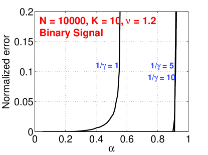
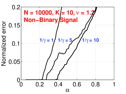
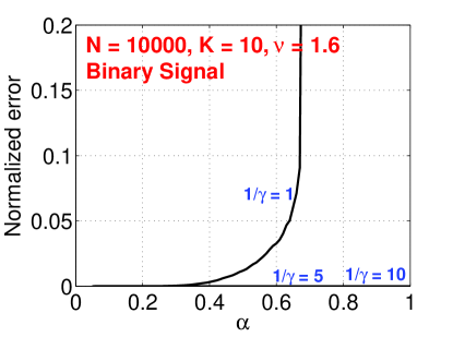
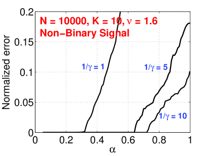
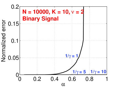
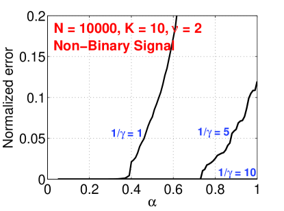
Figure 1: Normalized estimation errors (14) with $N=10000$ and $K=10$.

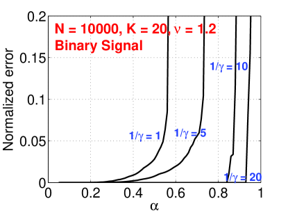
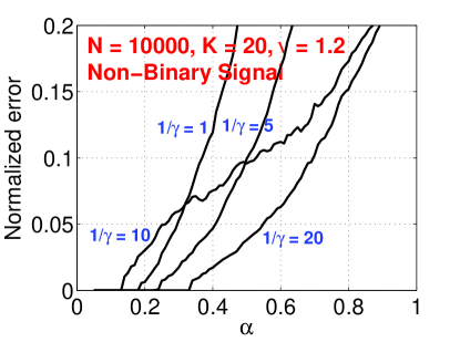
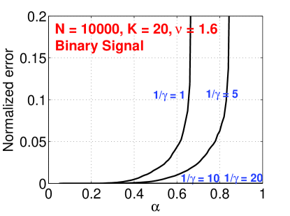
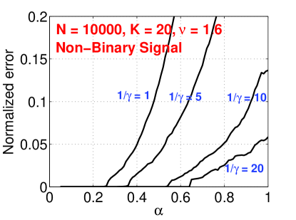
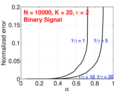
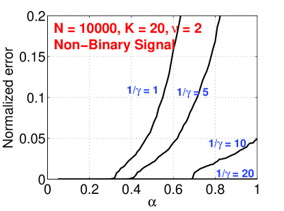
Figure 2: Normalized estimation errors (14) with $N=10000$ and $K=20$.

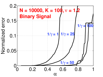
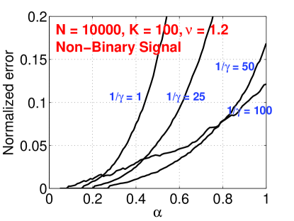
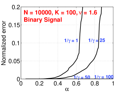
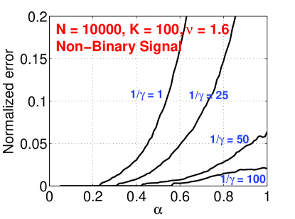
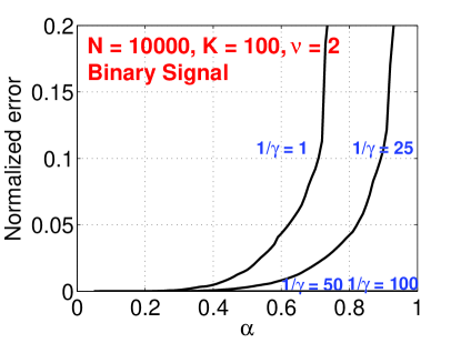
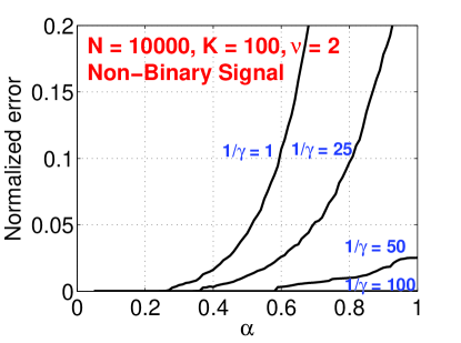
Figure 3: Normalized estimation errors (14) with $N=10000$ and $K=100$.

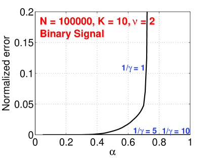
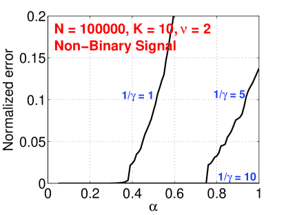
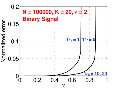
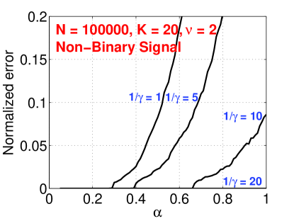
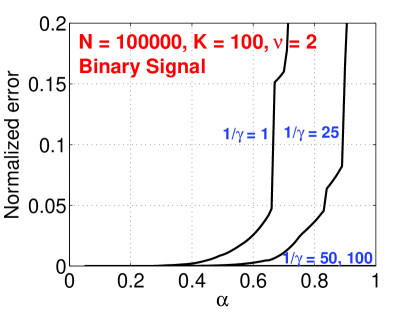
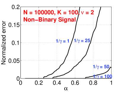
Figure 4: Normalized estimation errors (14) with $N=100000$ and $\nu=2$.

3 Analysis

Recall, we collect our measurements as

$$y_{j}=\sum_{i=1}^{N}x_{i}s_{ij}r_{ij},\ \ \ j=1,2,...,M$$ (15)

where $s_{ij}\sim S(\alpha,1,1)$ i.i.d. and

$$r_{ij}=\left\{\begin{array}[]{ll}1&\text{ with prob. }\gamma\\ 0&\text{ with prob. }1-\gamma\end{array}\right.\ \ \ i.i.d.$$ (18)

And any $s_{ij}$ and $r_{ij}$ are also independent. Our proposed estimator is simply

$$\hat{x}_{i,min,\gamma}=\min_{j\in T_{i}}\frac{y_{j}}{s_{ij}r_{ij}}$$ (19)

where $T_{i}$ is the set of nonzero entries in the $i$-th row of $S$, i.e.,

$$T_{i}=\{j,\ 1\leq j\leq M,\ r_{ij}=1\}$$ (20)

Conditional on $r_{ij}=1$,

$$\left.\frac{y_{j}}{s_{ij}r_{ij}}\right|r_{ij}=1=\frac{\sum_{t=1}^{N}x_{t}s_{tj}r_{tj}}{s_{ij}}=x_{i}+\frac{\sum_{t\neq i}^{N}x_{t}s_{tj}r_{tj}}{s_{ij}}=x_{i}+\left(\eta_{ij}\right)^{1/\alpha}\frac{S_{2}}{S_{1}}$$ (21)

where $S_{1},S_{2}\sim S(\alpha,1,1)$, i.i.d., and

$$\eta_{ij}=\sum_{t\neq i}^{N}\left(x_{t}r_{tj}\right)^{\alpha}=\sum_{t\neq i}^{N}x_{t}^{\alpha}r_{tj}$$ (22)

Note that

$$E(\eta_{ij})=\gamma\sum_{t\neq i}^{N}x_{tj}^{\alpha}\leq\gamma\sum_{t=1}^{N}x_{tj}^{\alpha},\hskip 21.68121pt\lim_{\alpha\rightarrow 0+}E(\eta_{ij})\leq\gamma K$$ (23)

When the signals are binary, i.e., $x_{i}\in\{0,\ 1\}$, we have

$$\eta_{ij}\sim\left\{\begin{array}[]{ll}Binomial(K,\ \gamma)&\text{ if }\ \ x_{i}=0\\ Binomial(K-1,\ \gamma)&\text{ if }\ \ x_{i}=1\end{array}\right.$$ (26)

The key in our theoretical analysis is the distribution of the ratio of two independent stable random variables. Here, we consider $S_{1},S_{2}\sim S(\alpha,1,1)$, i.i.d., and define

$$F_{\alpha}(t)=\mathbf{Pr}\left(\left({S_{2}}/{S_{1}}\right)^{\alpha/(1-\alpha)}\leq t\right),\hskip 14.45377ptt\geq 0$$ (27)

There is a standard procedure to sample from $S(\alpha,1,1)$ [3]. We first generate an exponential random variable with mean 1, $w\sim\exp(1)$, and a uniform random variable $u\sim unif\left(0,\pi\right)$, and then compute

$$\frac{\sin\left(\alpha u\right)}{\left[\sin u\cos\left(\alpha\pi/2\right)\right]^{\frac{1}{\alpha}}}\left[\frac{\sin\left(u-\alpha u\right)}{w}\right]^{\frac{1-\alpha}{\alpha}}\sim S(\alpha,1,1)$$ (28)

Lemma 1

[11] For any $t\geq 0$, $S_{1},S_{2}\sim S(\alpha,1,1)$, i.i.d.,

$$F_{\alpha}(t)=\mathbf{Pr}\left(\left({S_{2}}/{S_{1}}\right)^{\alpha/(1-\alpha)}\leq t\right)=\frac{1}{\pi^{2}}\int_{0}^{\pi}\int_{0}^{\pi}\frac{1}{1+Q_{\alpha}/t}du_{1}du_{2}$$ (29)

where

$$Q_{\alpha}=\left[\frac{\sin\left(\alpha u_{2}\right)}{\sin\left(\alpha u_{1}\right)}\right]^{\alpha/(1-\alpha)}\left[\frac{\sin u_{1}}{\sin u_{2}}\right]^{\frac{1}{1-\alpha}}\frac{\sin\left(u_{2}-\alpha u_{2}\right)}{\sin\left(u_{1}-\alpha u_{1}\right)}$$ (30)

In particular,

$$\lim_{\alpha\rightarrow 0+}F_{\alpha}(t)=\frac{1}{1+1/t},\hskip 36.135ptF_{0.5}(t)=\frac{2}{\pi}\tan^{-1}\sqrt{t}\hskip 36.135pt\hfill\Box$$ (31)

3.1 Error Probability

The following Lemma derives the general formula (32) for the error probability in terms of an expectation, which in general does not have a close-form solution. Nevertheless, when $\alpha=0+$ and $\alpha=0.5$, we can derive two convenient upper bounds, (34) and (36), respectively, which however are not tight.

Lemma 2

$$\mathbf{Pr}\left(\hat{x}_{i,min,\gamma}>x_{i}+\epsilon\right)= \left[1-\gamma E\left\{F_{\alpha}\left(\left(\frac{\epsilon^{\alpha}}{\eta_{ij}}\right)^{1/(1-\alpha)}\right)\right\}\right]^{M}$$ (32)

When $\alpha\rightarrow 0+$, we have

$$\mathbf{Pr}\left(\hat{x}_{i,min,\gamma}>x_{i}+\epsilon\right)\leq \left[1-\frac{1}{1/\gamma+K-1+1_{x_{i}=0}}\right]^{M}$$ (33)

$$\leq \left[1-\frac{1}{1/\gamma+K}\right]^{M}$$ (34)

When $\alpha=0.5$, we have

$$\mathbf{Pr}\left(\hat{x}_{i,min,\gamma}>x_{i}+\epsilon\right)\leq \left[1-\gamma\frac{2}{\pi}\tan^{-1}\left(\frac{\sqrt{\epsilon}}{\gamma\sum_{t\neq i}^{N}x_{t}^{1/2}}\right)\right]^{M}$$ (35)

$$\leq \left[1-\gamma\frac{2}{\pi}\tan^{-1}\left(\frac{\sqrt{\epsilon}}{\gamma\sum_{t=1}^{N}x_{t}^{1/2}}\right)\right]^{M}$$ (36)

Proof:      See Appendix A.$\hfill\Box$

It turns out, when $\alpha=0+$, we can precisely evaluate the expectation (32) and derive an accurate complexity bound (37) in Lemma 3.

Lemma 3

As $\alpha\rightarrow 0+$, we have

$$\mathbf{Pr}\left(\hat{x}_{i,min,\gamma}>x_{i}+\epsilon\right)= \left[1-\frac{1}{K+1_{x_{i}=0}}\left(1-(1-\gamma)^{K+1_{x_{i}=0}}\right)\right]^{M}$$ (37)

$$\leq \left[1-\frac{1}{K+1}\left(1-(1-\gamma)^{K+1}\right)\right]^{M}$$ (38)

$$\leq \left[1-\frac{1}{1/\gamma+K}\right]^{M}$$ (39)

Proof:      See Appendix B.$\hfill\Box$

3.2 Sample Complexity when $\alpha\rightarrow 0+$

Based on the precise error probability (37) in Lemma 3, we can derive the sample complexity bound from

$$(N-K)\left[1-\frac{1}{K+1}\left(1-(1-\gamma)^{K+1}\right)\right]^{M}+K\left[1-\frac{1}{K}\left(1-(1-\gamma)^{K}\right)\right]^{M}\leq\delta$$ (40)

Because $\left[1-\frac{1}{K}\left(1-(1-\gamma)^{K}\right)\right]^{M}\leq\left[1-\frac{1}{K+1}\left(1-(1-\gamma)^{K+1}\right)\right]^{M}$, it suffices to let

$$N\left[1-\frac{1}{K+1}\left(1-(1-\gamma)^{K+1}\right)\right]^{M}\leq\delta$$

This immediately leads to the sample complexity result for $\alpha\rightarrow 0+$ in Theorem 1.

Theorem 1

As $\alpha\rightarrow 0+$, the required number of measurements is

$$M=\frac{1}{-\log\left[1-\frac{1}{K+1}\left(1-(1-\gamma)^{K+1}\right)\right]}\log N/\delta$$ (41)

$\hfill\Box$

Remark:   The required number of measurements (41) can essentially be written as

$$M=\frac{K}{1-e^{-\gamma K}}\log N/\delta$$ (42)

The difference between (41) and (42) is very small even when $K$ is small, as shown in Figure 5. Let $\lambda=\gamma K$. If $\lambda=1$ (i.e., $\gamma=1/K$), then the required $M$ is about $1.58K\log N/\delta$. If $\lambda=2$ (i.e., $\gamma=2/K$), then $M$ is about $1.16K\log N/\delta$. In other words, we can use a very sparse design matrix and the required number of measurements is only inflated slightly.

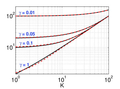
Figure 5: Solid curves: $\frac{1}{-\log\left[1-\frac{1}{K+1}\left(1-(1-\gamma)^{K+1}\right)\right]}$. Dashed curves: $\frac{K}{1-e^{-\gamma K}}$. The difference between (41) and (42) is very small even for small $K$. For large $K$, both terms approach $K$.

3.3 Worst-Case Sample Complexity

Theorem 2

If we choose $\gamma=\frac{1}{K+1}$, then it suffices to choose the number of measurements by

$$M=\frac{1}{-\log\left[1-\frac{1}{K+1}\left(1-\frac{1}{K+1}\right)^{K}\right]}\log N/\delta$$ (43)

Proof:   See Appendix C.$\hfill\Box$

Remark:   The worst-case complexity (43) can essentially be written as

$$M=eK\log N/\delta,\hskip 21.68121pt\text{ if }\gamma=1/K$$ (44)

where $e=2.7183...$ The previous analysis of sample complexity for $\alpha\rightarrow 0+$ says that if $\gamma=1/K$, it suffices to let $M=1.58K\log N/\delta$, and if $\gamma=2/K$, it suffices to let $M=1.15K\log N/\delta$. This means that the worst-case analysis is quite conservative and the choice $\gamma=1/K$ is not optimal for general $\alpha\in(0,1)$.

Interestingly, it turns out that the worst-case sample complexity is attained when $\alpha\rightarrow 1-$.

3.4 Sample Complexity when $\alpha=1-$

Theorem 3

For a $K$-sparse signal whose nonzero coordinates are larger than $\epsilon$, i.e., $x_{i}>\epsilon$ if $x_{i}>0$. If we choose $\gamma=\frac{1}{K+1}$, as $\alpha\rightarrow 1-$, it suffices to choose the number of measurements by

$$M=\frac{1}{-\log\left(1-\frac{1}{K+1}\left(1-\frac{1}{K+1}\right)^{K}\right)}\log N/\delta$$ (45)

Proof:      The proof can be directly inferred from the proof of Theorem 2 at $\alpha=1-$.$\hfill\Box$

Remark:      Note that, if the assumption $x_{i}>\epsilon$ whenever $x_{i}>0$ does not hold, then the required number of measurements will be smaller.

3.5 Sample Complexity Analysis for Binary Signals

As this point, we know the precise sample complexities for $\alpha=0+$ and $\alpha=1-$. And we also know the worst-case complexity. Nevertheless, it would be still interesting to study how the complexity varies as $\alpha$ changes between 0 and 1. While a precise analysis is difficult, we can perform an accurate analysis at least for binary signals, i.e., $x_{i}\in\{0,1\}$. For convenience, we first re-write the general error probability as

$$\mathbf{Pr}\left(\hat{x}_{i,min,\gamma}>x_{i}+\epsilon\right)=\left[1-\frac{1}{K}\left(\gamma K\right)E\left\{F_{\alpha}\left(\left(\frac{\epsilon^{\alpha}}{\eta_{ij}}\right)^{1/(1-\alpha)}\right)\right\}\right]^{M}$$ (46)

For binary signals, we have $\eta_{ij}\sim Binomial(K-1+1_{x_{i}=0},\gamma)$. Thus, if $x_{i}=0$, then

$$H=H(\gamma,K;\epsilon,\alpha)\overset{\bigtriangleup}{=} (\gamma K)E\left\{F_{\alpha}\left(\left(\frac{\epsilon^{\alpha}}{\eta_{ij}}\right)^{1/(1-\alpha)}\right)\right\}$$

$$= (\gamma K)\sum_{k=0}^{K}F_{\alpha}\left(\left(\frac{\epsilon^{\alpha}}{k}\right)^{1/(1-\alpha)}\right)\binom{K}{k}\gamma^{k}(1-\gamma)^{K-k}$$ (47)

The required number of measurements can be written as $\frac{1}{-\log\left(1-H/K\right)}\log N/\delta$, or essentially $\frac{K}{H}\log N/\delta$. We can compute $H(\gamma,K;\epsilon,\alpha)$ for given $\gamma$, $K$, $\epsilon$, and $\alpha$, at least by simulations.

4 Poisson Approximation for Complexity Analysis with Binary Signals

Again, the purpose is to study more precisely how the sample complexity varies with $\alpha\in(0,1)$, at least for binary signals. In this case, when $x_{i}=0$, we have $\eta_{ij}\sim Binomail(K,\gamma)$. Elementary statistics tells us that we can well approximate this binomial with a Poisson distribution with parameter $\lambda=\gamma K$ especially when $K$ is not small. Using the Poisson approximation, we can replace $H(\gamma,K;\epsilon,\alpha)$ in (47) by $h(\lambda;\epsilon,\alpha)$ and re-write the error probability as

$$\mathbf{Pr}\left(\hat{x}_{i,min,\gamma}>x_{i}+\epsilon\right)= \left[1-\frac{1}{K}h(\lambda;\epsilon,\alpha)\right]^{M}$$ (48)

where

$$h(\lambda;\epsilon,\alpha)= \lambda\sum_{k=0}^{\infty}F_{\alpha}\left(\left(\frac{\epsilon^{\alpha}}{k}\right)^{1/(1-\alpha)}\right)\frac{e^{-\lambda}\lambda^{k}}{k!}$$

$$= \lambda e^{-\lambda}+\lambda e^{-\lambda}\sum_{k=1}^{\infty}F_{\alpha}\left(\left(\frac{\epsilon^{\alpha}}{k}\right)^{1/(1-\alpha)}\right)\frac{\lambda^{k}}{k!}$$ (49)

which can be computed numerically for any given $\lambda$ and $\epsilon$.

The required number of measurements can be computed from

$$N\left[1-\frac{1}{K}h(\lambda;\epsilon,\alpha)\right]^{M}=\delta\Longleftrightarrow M=\frac{\log N/\delta}{-\log\left[1-\frac{1}{K}h(\lambda;\epsilon,\alpha)\right]}$$ (50)

for which it suffices to choose $M$ such that

$$M=\frac{K}{h(\lambda;\epsilon,\alpha)}\log N/\delta$$ (51)

Therefore, we hope $h(\lambda;\epsilon,\alpha)$ should be as large as possible.

4.1 Analysis for $\alpha=0.5$

Before we demonstrate the results via Poisson approximation for general $0<\alpha<1$, we would like to illustrate the analysis particularly for $\alpha=0.5$, which is a case readers can more easily verify.

Recall when $\alpha=0.5$, the error probability can be written as

$$\mathbf{Pr}\left(\hat{x}_{i,min,\gamma}>x_{i}+\epsilon\right)=\left[1-\frac{1}{K}\left(\gamma K\right)E\left\{\frac{2}{\pi}\tan^{-1}\left(\left(\frac{\sqrt{\epsilon}}{\eta_{ij}}\right)\right)\right\}\right]^{M}=\left[1-\frac{1}{K}H(\gamma,K;\epsilon,0.5)\right]^{M}$$

where

$$H(\gamma,K;\epsilon,0.5)=(\gamma K)\frac{2}{\pi}\sum_{k=0}^{K}\tan^{-1}\left(\frac{\sqrt{\epsilon}}{k}\right)\binom{K}{k}\gamma^{k}(1-\gamma)^{K-k}$$ (52)

From Lemma 2, in particular (36), we know there is a convenient lower bound of $H$:

$$H(\gamma,K;\epsilon,0.5)\geq H^{lower}(\gamma,K;\epsilon,0.5)=(\gamma K)\left\{\frac{2}{\pi}\tan^{-1}\left(\frac{\sqrt{\epsilon}}{\gamma K}\right)\right\}=\lambda\frac{2}{\pi}\tan^{-1}\left(\frac{\sqrt{\epsilon}}{\lambda}\right)$$ (53)

We will compare the precise $H(\gamma,K;\epsilon,0.5)$ with its lower bound $H^{lower}(\gamma,K;\epsilon,0.5)$, along with the Poisson approximation:

$$H(\gamma,K;\epsilon,0.5)\approx h(\lambda;\epsilon,0.5)=\lambda e^{-\lambda}\frac{2}{\pi}\sum_{k=0}^{\infty}\tan^{-1}\left(\frac{\sqrt{\epsilon}}{k}\right)\frac{\lambda^{k}}{k!}$$ (54)

Figure 6 confirms that the Poisson approximation is very accurate unless $K$ is very small, while the lower bound is conservative especially when $\gamma$ is around the optimal value. For small $\epsilon$, the optimal $\gamma$ is around $1/K$, which is consistent with the general worst-case complexity result.

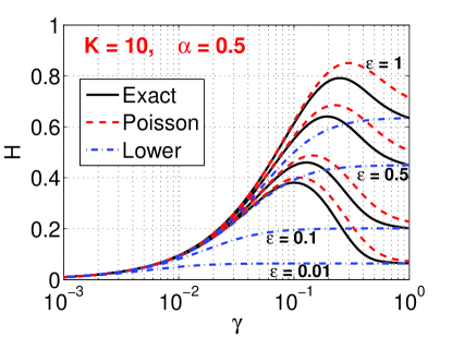
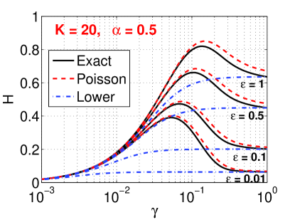
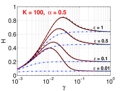
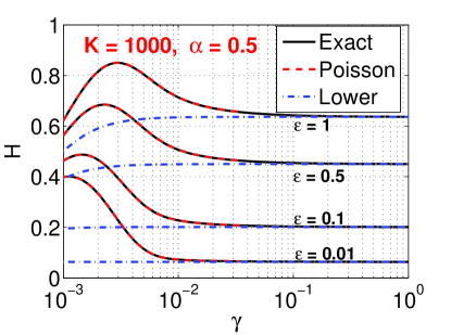
Figure 6: $H(\gamma,K;\epsilon,0.5)$ at four different values of $\epsilon\in\{0.01,0.1,0.5,1\}$. The exact $H$ and its Poisson approximation $h(\lambda;\epsilon,0.5)$ match very well unless $K$ is very small. The lower bound of $H$ is conservative, especially when $\gamma$ is around the optimal value. For small $\epsilon$, the optimal $\gamma$ is around $1/K$.

4.2 Poisson Approximation for General $0<\alpha<1$

Once we are convinced that the Poisson approximation is reliable at least for $\alpha=0.5$, we can use this tool to study for general $\alpha\in(0,1)$. Again, assume the Poisson approximation, we have

$$\mathbf{Pr}\left(\hat{x}_{i,min,\gamma}>x_{i}+\epsilon\right)= \left[1-\frac{1}{K}h(\lambda;\epsilon,\alpha)\right]^{M}$$

where

$$h(\lambda;\epsilon,\alpha)=\lambda e^{-\lambda}+\lambda e^{-\lambda}\sum_{k=1}^{\infty}F_{\alpha}\left(\left(\frac{\epsilon^{\alpha}}{k}\right)^{1/(1-\alpha)}\right)\frac{\lambda^{k}}{k!}$$

The required number of measurements can be computed from $M=\frac{K}{h(\lambda;\epsilon,\alpha)}\log N/\delta$.

As shown in Figure 7, at fixed $\epsilon$ and $\lambda$, the optimal (highest) $h$ is larger when $\alpha$ is smaller. The optimal $h$ occurs at larger $\lambda$ when $\alpha$ is closer to zero and at smaller $\lambda$ when $\alpha$ is closer to 1.

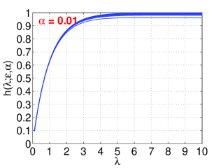
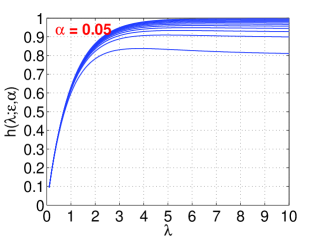
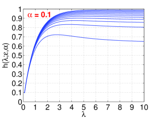
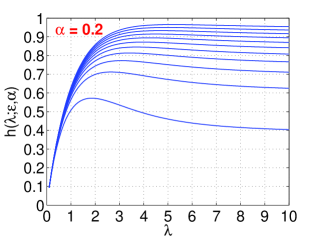
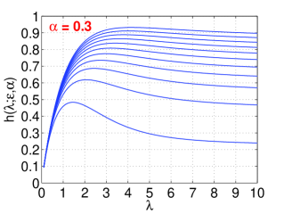
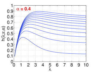
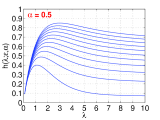
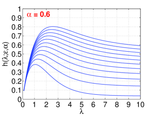
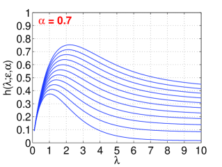
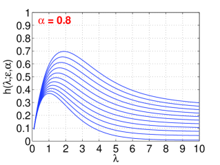
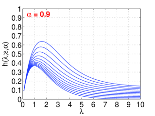
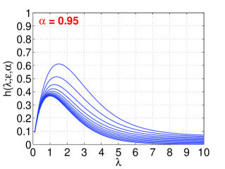
Figure 7: $h(\lambda;\epsilon,\alpha)$ as defined in (49) for selected $\alpha$ values ranging from $0.01$ to $0.95$. In each panel, each curve corresponds to an $\epsilon$ value, where $\epsilon\in\{0.01,0.1,0.2,0.3,0.4,0.5,0.6,0.7,0.8,0.9,1\}$ (from bottom to top). In each panel, the curve for $\epsilon=0.01$ is the lowest and the curve for $\epsilon=1$ is the highest.

Figure 8 plots the optimal (smallest) $1/h(\lambda;\epsilon,\alpha)$ values (left panel) and the optimal $\lambda$ values (right panel) which achieve the optimal $h$.

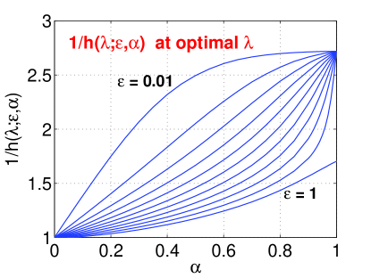
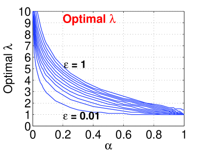
Figure 8: Left Panel: $1/h(\lambda;\epsilon,\alpha)$ at the optimal $\lambda$ values. Right Panel: the optimal $\lambda$ values.

Figure 9 plots $1/h(\lambda;\epsilon,\alpha)$ for fixed $\lambda=1$ (left panel) and $\lambda=2$ (right panel), together with the optimal $1/h(\lambda;\epsilon,\alpha)$ values (dashed curves).

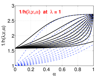
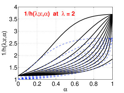
Figure 9: $1/h(\lambda;\epsilon,\alpha)$ at the fixed $\lambda=1$ (left panel) and $\lambda=2$ (right panel). The dashed curves correspond to $1/h(\lambda;\epsilon,\alpha)$ at the optimal $\lambda$ values.

4.3 Poisson Approximation for $\alpha\rightarrow 1-$

We now examine $h(\lambda;\epsilon,\alpha)$ closely at $\alpha=1-$, i.e., $\frac{1}{1-\alpha}\rightarrow\infty$.

$$h(\lambda;\epsilon,\alpha)=\lambda e^{-\lambda}+\lambda e^{-\lambda}\sum_{k=1}^{\infty}F_{\alpha}\left(\left(\frac{\epsilon^{\alpha}}{k}\right)^{1/(1-\alpha)}\right)\frac{\lambda^{k}}{k!}$$

Interestingly, when $\epsilon=1$, only $k=0$ and $k=1$ will be useful, because otherwise $\left(\frac{\epsilon^{\alpha}}{k}\right)^{1/(1-\alpha)}\rightarrow\infty$ as $\Delta=1-\alpha\rightarrow 0$. When $\epsilon<1$, then only $k=0$ is useful. Thus, we can write

$$h(\lambda;\epsilon<1,\alpha=1-)=\lambda e^{-\lambda}$$ (55)

$$h(\lambda;\epsilon=1,\alpha=1-)=\lambda e^{-\lambda}+\lambda^{2}e^{-\lambda}F_{1-}\left(1\right)=\lambda e^{-\lambda}+\lambda^{2}e^{-\lambda}/2$$ (56)

Notes that $F_{1-}(1)=1/2$ due to symmetry.

This mean, the maximum of $h(\lambda;\epsilon<1,\alpha=1-)$ is $e^{-1}$ attained at $\lambda=1$, and the maximum of $h(\lambda;\epsilon=1,\alpha=1-)$ is $e^{-\sqrt{2}}(1+\sqrt{2})=0.5869$, attained at $\lambda=\sqrt{2}$, as confirmed by Figure 10. In other words, it suffices to choose the number of measurements to be

$$M=eK\log N/\delta\hskip 7.22743pt\text{ if }\epsilon<1,\hskip 36.135ptM=1.7038K\log N/\delta\hskip 7.22743pt\text{ if }\epsilon=1$$ (57)

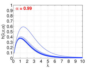
Figure 10: $h(\lambda;\epsilon,\alpha)$ as defined in (49) for $\alpha$ close to 1. As $\alpha\rightarrow 1-$, the maximum of $h(\lambda;\epsilon,\alpha)$ approaches $e^{-1}$ attained at $\lambda=1$, for all $\epsilon<1$. When $\epsilon=1$, the maximum approaches 0.5869, attained at $\lambda=\sqrt{2}$.

5 Conclusion

In this paper, we extend the prior work on Compressed Counting meets Compressed Sensing [11] and very sparse stable random projections [9, 6] to the interesting problem of sparse recovery of nonnegative signals. The design matrix is highly sparse in that on average only $\gamma$-fraction of the entries are nonzero; and we sample the nonzero entries from an $\alpha$-stable maximally-skewed distribution where $\alpha\in(0,1)$. Our theoretical analysis demonstrates that the design matrix can be extremely sparse, e.g., $\gamma=\frac{1}{K}\sim\frac{2}{K}$. In fact, when $\alpha$ is away from 0, it is much more preferable to use a very sparse design.

Appendix A Proof of Lemma 2

$$\mathbf{Pr}\left(\hat{x}_{i,min,\gamma}>x_{i}+\epsilon\right)$$

$$= E\left(\mathbf{Pr}\left(\frac{y_{j}}{s_{ij}}>x_{i}+\epsilon,\ j\in T_{i}|T_{i}\right)\right)$$

$$= E\prod_{j\in T_{i}}\left[\mathbf{Pr}\left(\frac{S_{2}}{S_{1}}>\frac{\epsilon}{\eta_{ij}^{1/\alpha}}\right)\right]$$

$$= E\prod_{j\in T_{i}}\left[1-F_{\alpha}\left(\left(\frac{\epsilon^{\alpha}}{\eta_{ij}}\right)^{1/(1-\alpha)}\right)\right]$$

$$= E\left\{\left[1-E\left\{F_{\alpha}\left(\left(\frac{\epsilon^{\alpha}}{\eta_{ij}}\right)^{1/(1-\alpha)}\right)\right\}\right]^{|T_{i}|}\right\}$$

$$= \left[1-\gamma+\gamma\left\{1-E\left\{F_{\alpha}\left(\left(\frac{\epsilon}{\eta_{ij}}\right)^{\alpha/(1-\alpha)}\right)\right\}\right\}\right]^{M}$$

$$= \left[1-\gamma E\left\{F_{\alpha}\left(\left(\frac{\epsilon^{\alpha}}{\eta_{ij}}\right)^{1/(1-\alpha)}\right)\right\}\right]^{M}$$

When $\alpha=0.5$, we have $F_{\alpha}(t)=\frac{2}{\pi}\tan^{-1}\sqrt{t}$ and hence

$$\mathbf{Pr}\left(\hat{x}_{i,min,\gamma}>x_{i}+\epsilon\right)$$

$$= \left[1-\gamma E\left\{F_{\alpha}\left(\left(\frac{\epsilon^{\alpha}}{\eta_{ij}}\right)^{1/(1-\alpha)}\right)\right\}\right]^{M}$$

$$= \left[1-\gamma E\left\{\frac{2}{\pi}\tan^{-1}\left(\left(\frac{\sqrt{\epsilon}}{\eta_{ij}}\right)\right)\right\}\right]^{M}$$

$$\leq \left[1-\gamma\left\{\frac{2}{\pi}\tan^{-1}\left(\left(\frac{\sqrt{\epsilon}}{E\eta_{ij}}\right)\right)\right\}\right]^{M}\hskip 21.68121pt(\text{Jensen's Inequality})$$

$$\leq \left[1-\gamma\left\{\frac{2}{\pi}\tan^{-1}\left\{\frac{1}{\gamma}\frac{\sqrt{\epsilon}}{\sum_{t\neq i}x_{t}^{1/2}}\right\}\right\}\right]^{M}$$

When $\alpha=0+$, we have $F_{0+}(t)=\frac{1}{1+1/t}$ and hence

$$\mathbf{Pr}\left(\hat{x}_{i,min,\gamma}>x_{i}+\epsilon\right)$$

$$= \lim_{\alpha\rightarrow 0+}\left[1-\gamma E\left\{F_{0+}\left(\frac{1}{\eta_{ij}}\right)\right\}\right]^{M}$$

$$= \lim_{\alpha\rightarrow 0+}\left[1-\gamma E\left\{\left(\frac{1}{1+\eta_{ij}}\right)\right\}\right]^{M}$$

$$\leq \lim_{\alpha\rightarrow 0+}\left[1-\gamma\left\{\left(\frac{1}{1+E\eta_{ij}}\right)\right\}\right]^{M}$$

$$\leq \lim_{\alpha\rightarrow 0+}\left[1-\gamma\frac{1}{1+\gamma K}\right]^{M}$$

$$= \left[1-\frac{1}{1/\gamma+K}\right]^{M}$$

This completes the proof.

Appendix B Proof of Lemma 3

Proof:   When $\alpha=0+$, we have $F_{0+}(t)=\frac{1}{1+1/t}$ and hence

$$\mathbf{Pr}\left(\hat{x}_{i,min,\gamma}>x_{i}+\epsilon\right)=\lim_{\alpha\rightarrow 0+}\left[1-\gamma E\left\{\left(\frac{1}{1+\eta_{ij}}\right)\right\}\right]^{M}$$

Suppose $x_{i}=0$, then as $\alpha\rightarrow 0+$, $\eta_{ij}\sim Binomial(K,\gamma)$, and

$$E\left(\frac{1}{1+\eta_{ij}}\right)$$

$$= \sum_{n=0}^{K}\frac{1}{1+n}\binom{K}{n}\gamma^{n}(1-\gamma)^{K-n}$$

$$= \sum_{n=0}^{K}\frac{1}{1+n}\frac{K!}{n!(K-n)!}\gamma^{n}(1-\gamma)^{K-n}$$

$$= \sum_{n=0}^{K}\frac{K!}{(n+1)!(K-n)!}\gamma^{n}(1-\gamma)^{K-n}$$

$$= \frac{1}{K+1}\frac{1}{\gamma}\sum_{n=0}^{K}\frac{(K+1)!}{(n+1)!((K+1)-(n+1))!}\gamma^{n+1}(1-\gamma)^{(K+1)-(n+1)}$$

$$= \frac{1}{K+1}\frac{1}{\gamma}\sum_{n=1}^{K+1}\frac{(K+1)!}{(n)!((K+1)-(n))!}\gamma^{n}(1-\gamma)^{(K+1)-(n)}$$

$$= \frac{1}{K+1}\frac{1}{\gamma}\left\{\sum_{n=0}^{K+1}\frac{(K+1)!}{(n)!((K+1)-(n))!}\gamma^{n}(1-\gamma)^{(K+1)-(n)}-(1-\gamma)^{K+1}\right\}$$

$$= \frac{1}{K+1}\frac{1}{\gamma}\left\{1-(1-\gamma)^{K+1}\right\}$$

Similarly, suppose $x_{i}>0$, we have

$$E\left(\frac{1}{1+\eta_{ij}}\right)=\frac{1}{K}\frac{1}{\gamma}\left\{1-(1-\gamma)^{K}\right\}$$

Therefore, as $\alpha\rightarrow 0+$, when $x_{i}=0$, we have

$$\mathbf{Pr}\left(\hat{x}_{i,min,\gamma}>x_{i}+\epsilon\right)=\left[1-\frac{1}{K+1}\left(1-(1-\gamma)^{K+1}\right)\right]^{M}$$

and when $x_{i}>0$, we have

$$\mathbf{Pr}\left(\hat{x}_{i,min,\gamma}>x_{i}+\epsilon\right)=\left[1-\frac{1}{K}\left(1-(1-\gamma)^{K}\right)\right]^{M}$$

To conclude the proof, we need to show

$$\left[1-\frac{1}{K+1}\left(1-(1-\gamma)^{K+1}\right)\right]^{M}\leq\left[1-\frac{1}{1/\gamma+K}\right]^{M}$$

$$\Longleftrightarrow \frac{1}{K+1}\left(1-(1-\gamma)^{K+1}\right)\geq\frac{1}{1/\gamma+K}$$

$$\Longleftrightarrow h(\gamma,K)=1/\gamma-(1-\gamma)^{K+1}/\gamma-K(1-\gamma)^{K+1}-1\geq 0$$

Note that $0\leq\gamma\leq 1$, $h(0,K)=h(1,K)=h(\gamma,1)=0$. Furthermore

$$\frac{\partial h(\gamma,K)}{\partial K}= -(1-\gamma)^{K+1}\log(1-\gamma)/\gamma-(1-\gamma)^{K+1}-K(1-\gamma)^{K+1}\log(1-\gamma)$$

$$= -(1-\gamma)^{K+1}\left(\log(1-\gamma)/\gamma+1+K\log(1-\gamma)\right)\geq 0$$

as $\log(1-\gamma)/\gamma<-1$. Thus, $h(\gamma,K)$ is a monotonically increasing function of $K$ and this completes the proof.

Appendix C Proof of Theorem 2

$$\mathbf{Pr}\left(\hat{x}_{i,min,\gamma}>x_{i}+\epsilon\right)= \left[1-\gamma E\left\{F_{\alpha}\left(\left(\frac{\epsilon^{\alpha}}{\eta_{ij}}\right)^{1/(1-\alpha)}\right)\right\}\right]^{M}$$

$$\geq \left[1-\gamma\mathbf{Pr}\left(\eta_{ij}=0\right)\right]^{M}$$

$$= \left[1-\gamma\left(1-\gamma\right)^{K-1+1_{x_{i}=0}}\right]^{M}$$

$$\geq \left[1-\gamma\left(1-\gamma\right)^{K}\right]^{M}$$

The minimum of $\gamma\left(1-\gamma\right)^{K-1+1_{x_{i}=0}}$ is attained at $\gamma=\frac{1}{K+1_{x_{i}=0}}$. If we choose $\gamma^{*}=\frac{1}{K+1}$, then

$$\mathbf{Pr}\left(\hat{x}_{i,min,\gamma}>x_{i}+\epsilon\right)\geq \left[1-\gamma^{*}\left(1-\gamma^{*}\right)^{K}\right]^{M}=\left[1-\frac{1}{K+1}\left(1-\frac{1}{K+1}\right)^{K}\right]^{M}$$

and it suffices to choose $M$ so that

$$M=\frac{1}{-\log\left[1-\frac{1}{K+1}\left(1-\frac{1}{K+1}\right)^{K}\right]}\log N/\delta$$

This completes the proof.

References

[1]
R. Berinde, P. Indyk, and M. Ruzic.
Practical near-optimal sparse recovery in the l1 norm.
In Communication, Control, and Computing, 2008 46th Annual
Allerton Conference on, pages 198 –205, 2008.
[2]
Emmanuel Candès, Justin Romberg, and Terence Tao.
Robust uncertainty principles: exact signal reconstruction from
highly incomplete frequency information.
IEEE Trans. Inform. Theory, 52(2):489–509, 2006.
[3]
John M. Chambers, C. L. Mallows, and B. W. Stuck.
A method for simulating stable random variables.
Journal of the American Statistical Association,
71(354):340–344, 1976.
[4]
David L. Donoho.