Value of information in noncooperative games

Abstract

In some games, additional information hurts a player, e.g., in games with first-mover advantage, the second-mover is hurt by seeing the first-mover’s move. What properties of a game determine whether it has such negative “value of information” for a particular player? Can a game have negative value of information for all players? To answer such questions, we generalize the definition of marginal utility of a good to define the marginal utility of a parameter vector specifying a game. So rather than analyze the global structure of the relationship between a game’s parameter vector and player behavior, as in previous work, we focus on the local structure of that relationship. This allows us to prove that generically, every game can have negative marginal value of information, unless one imposes a priori constraints on allowed changes to the game’s parameter vector. We demonstrate these and related results numerically, and discuss their implications.

1 Introduction

How a player in a noncooperative game behaves typically depends on what information she has both about her physical environment and about the behavior of the other players. Accordingly, the joint behavior of multiple interacting players can depend strongly on the information available to the separate players, both about one another, and about Nature-based random variables. Precisely how the joint behavior of the players depends on this information is determined by the preferences of those players. So in general there is a strong interplay among the information structure connecting a set of players, the preferences of those players, and their behavior.

Previous analyses of this interplay have considered how player behavior changes under global, non-infinitesimal changes to the parameters specifying the underlying game. Here we pursue a different approach, generalizing the concept of “marginal value of a good” from the setting of a single decision-maker in a game against Nature to a multi-player setting. In other words, rather than consider the global structure of the relationship between the game parameters and player behavior, we focus on the local structure of that relationship.

This analysis of the local structure allows us construct general theorems on when there is a change to an information structure that will reduce information available to a player but increase their expected utility. It also allows us to construct extended “Pareto” versions of these theorems, specifying when there is a change to an information structure that will both reduce information available to all players and increase all of their expected utilities.

We illustrate these theoretical results with computer experiments involving the noisy leader-follower game. We also discuss the general implications of these results for well-known issues in the economics of information.

1.1 Value of information

Intuitively, it might seem that a rational decision maker cannot be hurt by additional information. After all, that is the standard interpretation of Blackwell’s famous result that adding noise to an observation by sending it through an additional channel, called garbling, cannot improve expected utility of a Bayesian decision maker in a game against Nature [7]. However games involving multiple players, and/or bounded rational behavior, might violate this intuition.

To investigate the legitimacy of this intuition for general noncooperative games, we first need to formalize what it means to have “additional information”. To begin, consider the simplest case, of a single-player game. We can compare two scenarios: One where the player can observe a relevant state of Nature, and another situation that is identical, except that now she cannot observe that state of Nature. More generally, we can compare a scenario where the player receives a noisy signal about the state of Nature to a scenario that is identical except that the signal she receives is strictly noisier (in a certain sense) than in the first scenario. Indeed, in his seminal paper [7], Blackwell proved that the set of changes to an information channel that can never increase the expected utility of the player are precisely those that are equivalent to sending the signal through an additional channel, and thereby introducing extra noise. So at least in a game against Nature, one can usefully define the “value of information” as the difference in highest expected utility that can be achieved in a low noise scenario (more information) compared to a high noise scenario (less information) [15], and prove important properties about this value of information.

In trying to extend this reasoning from a single player game to a multi-player game two complications arise. First, in a multi-player game there can be multiple equilibria, with different expected utilities from one another. All of those equilibria will change, in different ways, when noise is added to an information channel connecting players in the game. Indeed, even the number of equilibria may change when noise is added to a channel. This means there is no well-defined way to compare equilibrium behavior in a “before” scenario with equilibrium behavior in an “after” scenario in which noise has been added; there is arbitrariness in which pair of equilibria, one from each scenario, we use for the comparison. Note that there is no such ambiguity in a game against Nature. (In addition, this ambiguity does not arise in the Cournot scenarios discussed below if we restrict attention to subgame perfect equilibria.)

A second complication is that in a multi-player game all of the players will react to a change in an information channel, if not directly then indirectly, via the strategic nature of the game. This effect can even result in a negative value of information, in that it means a player would prefer less (i.e., noisier) information. Indeed, such negative value of information can arise even when both the “before” and “after” scenarios have unique (subgame perfect) equilibria, so that there is no ambiguity in choosing which two equilibria to compare.

To illustrate this, consider the Cournot duopoly where two competing manufacturers of a good simultaneously choose a production level. Note that, as far as its equilibrium structure is concerned, this scenario is equivalent to one player — the “leader” — choosing his production level first, but the other player, the “follower”, having no information about the leader’s choice before making her choice. Assuming that both players can produce the good for the same cost and that the demand function is linear, it is well known that in that equilibrium both players get the same profit.

Now change the game by having the follower observe the leader’s move before she moves. So the only change is that the follower now has more information before making her move. In this new game, the leader can choose a higher production level compared to the production level of the simultaneous move game — the monopoly production level — and the follower has to react by choosing a lower production level. Thus, the follower is actually hurt by this change to the game that results in her having more information.

In this example, the leader changes his move to account for the information that (he knows that) the follower will receive. Then, after receiving this information, the follower cannot credibly ignore it, i.e., cannot credibly behave as in the simultaneous move game equilibrium. So this equilibrium of the new game, where the follower is hurt by the extra information, is subgame-perfect. These and several other examples of negative value of information can be found in the game theory literature (see section 1.6 for references).

In this paper we introduce a broad framework that overcomes these two complications which distinguish multi-player games from single-player games. This framework is based on generalizing the concept of the “marginal value of a good”, to a decision-maker in a game against Nature, so that it can apply to multi-player game scenarios. This means that in our approach, the “before” and “after” scenarios traditionally used to define value of information in games against Nature are infinitesimally close to one another. More precisely, we consider how much the expected utility of a player changes per unit change in the amount of information as one infinitesimally changes the conditional distribution specifying the information channel in a game. (This is illustrated in Fig. 1.) Interestingly, such a local picture is widely used in decision theory, i.e. marginal value, but has, to our knowledge not been considered in game theory. Instead, as in the example above, investigations of value of information have been based exclusively on comparing global changes to the information structure, e.g. no vs. full information.

Figure 1: Both the expected utility of player $i$ and the amount of information player $i$ receives depend, in part, on the strategy profile of all the players, $\boldsymbol{\sigma}$. Via the equilibrium concept, that profile in turn depends on the specific conditional distributions $\boldsymbol{\theta}$ in the information channel providing data to player $i$. So a change to $\boldsymbol{\theta}$ results in a coupled change to the expected utility of player $i$, ${\mathbb{E}}_{\boldsymbol{\theta}}[u_{i}]$, and to the amount of information in their channel, $f({\boldsymbol{\theta}})$. The “marginal value of information” to $i$ is how much ${\mathbb{E}}_{\boldsymbol{\theta}}(u_{i})$ changes per unit change in $f(\boldsymbol{\theta})$ if $\boldsymbol{\theta}$ is changed infinitesimally.

In the next subsection we provide a careful motivation for our “marginal value of information” approach. As we discuss in the following subsection, this requires us to choose a cardinal measure of amount of information as well as a way to relate infinitesimal changes in utility to infinitesimal changes in information. Next we discuss the broad benefits of our approach, e.g., as a way to quantify marginal rates of substitution of different kinds of information arising in a game. After this we relate our framework to previous work. We end this section by providing a roadmap to the rest of our paper.

1.2 From consumers making a choice to multi-player games

To motivate our framework, first consider the simple case of a consumer whose preference function depends jointly on the quantities of all the goods they get in a market. Given some current bundle of goods, how should we quantify the value they assign to getting more of good $j$? The usual economic answer is the marginal utility of good $j$ to the consumer, i.e., the derivative of their expected utility with respect to amount of good $j$.

Rather than ask what the marginal value of good $j$ is to the consumer, we might ask what their marginal value is for some linear combination of $j$ and a different good $j^{\prime}$. The natural answer is their “marginal value”, i.e. is the marginal utility of that precise linear combination of goods.

More generally, rather than considering the marginal value to the consumer of a linear combination of the goods, we might want to consider the marginal value to them of some arbitrary, perhaps non-linear function of quantities of each of the goods. What marginal value would they assign to that?

To ground our thinking, consider an example where the function is the total weight of all the goods. What would be the “value of weight”? To answer this question, write the bundle of goods the consumer possesses as $\boldsymbol{\theta}$, i.e. $\theta^{j}$ is the amount of good $j$. Then write the consumer’s expected utility as $V(\boldsymbol{\theta})$, and the weight of the bundle as the function $f(\boldsymbol{\theta})$. We want to relate how the utility changes when the weight of the bundle is changed infinitesimally.

In general, there is no unique such relation since the weight $f$ is a scalar-valued function and thus different changes $\delta\boldsymbol{\theta}$ to the bundle could lead to the same change in the weight of the bundle, even though they might result in different changes to the expected utility. So to answer our question we need to fix the direction of change $\delta\boldsymbol{\theta}$ to the bundle of goods. Once we have done that, then to first-order the utility changes by $\langle\mathtt{grad}V,\delta\boldsymbol{\theta}\rangle$ while the weight is changed by $\langle\mathtt{grad}f,\delta\boldsymbol{\theta}\rangle$.

Accordingly we define the “differential value of $f$ (in the direction $\delta\boldsymbol{\theta}$)” as

$$\frac{\langle\mathtt{grad}V,\delta\boldsymbol{\theta}\rangle}{\langle\mathtt{grad}f,\delta\boldsymbol{\theta}\rangle}$$ (1)

Thus, a change to the bundle has a high differential value of $f$, e.g. of weight, when that change (in the direction $\delta\boldsymbol{\theta}$) results in a large gain in utility for a small change in $f$.

In some situations one might wish to speak of the “value of $f$” without specifying a specific direction of change to the vector-valued argument of $f$. Indeed, all previous quantifications of “value of information” that we know of, both in game theory and in other fields (e.g., analysis of influence diagrams [15, 19]), quantifies value of information without specifying a direction.

We can extend our approach to provide such a “direction-free” quantification of value of information, by choosing the direction $\delta\boldsymbol{\theta}=\mathtt{grad}f$ which results in the largest change of $f$, i.e. steepest ascent. Thus, we can quantify the “differential value of $f$” as

$$\frac{\langle\mathtt{grad}(V),\mathtt{grad}f\rangle}{||\mathtt{grad}f||^{2}}$$ (2)

The measure in (2) says that if a small change in the value of $f$ leads to a big change in expected utility, $f$ is more valuable than if the same change in expected utility required a bigger change in the value of $f$. Furthermore, it expresses the value of information in units of value (of an infinitesimal change to $f$) per unit of $f$. Thus, we follow the conventional terminology where we would typically say that how much the consumer values a change to good $j$ is given by the associated change in utility divided by the amount of change in good $j$. (After all, that tells us change in utility per unit change in the good.)

All of the reasoning above can be carried over from the case of a single consumer to apply to multi-player scenarios. To see how, first note that in the reasoning above, $\boldsymbol{\theta}$ is simply the parameter vector determining the utility of the consumer. In other words, it is the parameter vector specifying the details of a game being played by a decision maker in a game against Nature. So it naturally generalizes to a multi-player game, as the parameter vector specifying the details of such a game.

Next, replace the consumer player in the reasoning above by a particular player in the multi-player game. The key to the reasoning above is that specifying $\boldsymbol{\theta}$ specifies the expected utility of the consumer player. In the case of the consumer, that map from parameter vector to expected utility is direct. In a multi-player game, that direct map becomes an indirect map specified in two stages: First by the equilibrium concept, taking $\boldsymbol{\theta}$ to the mixed strategy profile of all the players, and then from that profile to the expected utility of any particular player. (Cf., Fig. 1.)

As mentioned above though, there is an extra complication in the multi-player case that is absent in the case of the single consumer. Typically multi-player games have multiple equilibria for any $\boldsymbol{\theta}$, and therefore multiple values of $V(\boldsymbol{\theta})$. (In Fig. 1, the map from $\boldsymbol{\theta}$ to the mixed strategy profile is multi-valued in games with multiple players.) However we need to have the mapping from $\boldsymbol{\theta}$ to the expected utility of the players be single-valued to use the reasoning above. This means that we have to be careful when calculating derivatives to specify which precise branch of the set of equilibria we are considering. Having done that, our generalization from the definition of marginal utility for the case of a consumer choosing a bundle of goods to marginal utility for a player in a multi-player game is complete.

1.3 General comments on the marginal value approach

There are several aspects of this general framework that are important to emphasize. First, there is no reason to restrict attention to Nash equilibria (or some appropriate refinement). All that we need is that $\boldsymbol{\theta}$ specifies (a set of) equilibrium expected utilities for all the players. The equilibrium concept can be anything at all.

Second, note that $\boldsymbol{\theta}$, together with the solution concept and choice of an equilibrium branch, specifies the mixed strategy profile of the players, as well as all prior and conditional probabilities. So it specifies the distributions governing the joint distribution over all random variables in the game. Accordingly, it specifies the values of all cardinal functions of that joint distribution. So in particular, however we wish to quantify “amount of information”, so long as it is a function of that joint distribution, it is an indirect function of $\boldsymbol{\theta}$ (for a fixed solution concept and associated choice of a solution branch). This means we can apply our analysis for any such quantification of the amount of information as a function $f(\boldsymbol{\theta})$.

We have to make several choices every time we use our approach. One is that we must choose what parameters of the game to vary. In addition, when analyzing value of information in a particular direction, we have to specify that direction. Taken together these choices fix what economic question we are considering. Similar choices (e.g., of what game parameters to allow to vary) arise, either implicitly or explicitly, in any economic modeling. Furthermore, we must decide what information measures we wish to analyze. (We address this issue in the next subsection.)

Finally, if we wish to analyze value of information we confront an additional, purely formal choice, unique to analyses of marginal values. This is the choice of what coordinate system to use to evaluate the dot products and gradients in Eq. (2). The difficulty is that changing the coordinate system changes the values of both dot products and gradient vectors in general. So different choices of coordinate system would give different marginal values of information. However since the choice of coordinate system is purely a modeling choice, we do not want our conclusions to change if we change how we parametrize the noise level in a communication channel, for example.

To address this problem we need to introduce a metric, as in differential geometry. In different economic scenarios, different choices of metric may be appropriate. In general, they can change our results.

Here, for reasons of space, we concentrate on metric-independent results. Differential value of information at a particular $\boldsymbol{\theta}$ depends on the choice of metric in general. However the differential value of information in a given direction does not depend on the metric (or coordinate system) as explained in section 3. Accordingly, in this paper we restrict attention to differential value of information in a given direction.

1.4 How to quantify information

To use the framework outlined in Sec. 1.2, we must choose a function $f(\boldsymbol{\theta})$ that measures the amount of information in a game with parameter $\boldsymbol{\theta}$. Traditionally, a player’s information is represented in game theory by a signal that the player receives during the game. Thus information is often thought of as an object or commodity. But this general approach does not integrate the important fact that a signal is only informative to the extent that it changes what the player believes about some other aspect of the game. It is the relationship between the value of the signal and that other aspect of the game that determines the “amount of information” in the signal.

More precisely, let $y$, sampled from a distribution $p(y)$, be a payoff-relevant variable whose state player $i$ would like to know before making her move, but which she cannot observe directly. Say that the value $y$ is used to generate a datum/signal $x$, that the player directly observes, via a conditional distribution $p(x\mid y)$ which we typically refer to as an information channel. If for some reason the player ignored $x$, then she would assign the a-priori likelihood $p(y)$ to $y$, even though in fact its a-posteriori likelihood is $p(y\mid x)=\frac{p(y)p(x\mid y)}{\sum_{y^{\prime}}p(y^{\prime})p(x\mid y^{\prime})}$. This change in the likelihoods she would assign to $y$ is a measure of the information that $x$ provides about $y$. Arguably, this change of distribution is the core property of information that is of interest in economic scenarios.

Averaging over observation $x$ and state $y$’s, and working in log space, this change in the likelihood she would assign to the actual $y$ if she ignored $x$ (and so used likelihoods $p(y)$ rather than $p(y\mid x)$) is

$$\sum_{x,y}p(x)p(y\mid x)\ln\bigg{[}\frac{p(y\mid x)}{p(y)}\bigg{]}.$$ (3)

Thus, eq. (3) gives the (average) increase in information that player $i$ has about $y$ due to observing $x$. Note that this is true no matter how the variables $X$ and $Y$ arise in the strategic interaction. In particular, this interpretation of the quantity in Eq. (3) does not require that the value $x$ arise directly through a pre-specified distribution $p(x\mid y)$. $x$ and $y$ could instead be variables concerning the strategies of the players at a particular equilibrium.

In this sense, we have shown that the quantity in Eq. (3) is a proper way to measure the information relating any pair of variables arising in a strategic scenario. None of the usual axiomatic arguments motivating Shannon’s information theory [25, 11] were used in doing this. Nevertheless, the quantity in Eq. (3) is just the mutual information between $X$ and $Y$, as defined by Shannon. Mutual information, together with the related quantity of entropy, forms the basis of information theory. It not only allows us to quantify information, but has many applications in different areas ranging from coding theory to machine learning to evolutionary biology.

In game theory, information is more commonly expressed in terms of an information partition. An information partition $\{\mathcal{A}_{1},\ldots,\mathcal{A}_{n}\}$ (on some measure space $\Omega$) can be viewed as a random variable with values $x\in\mathcal{X}=\{1,\ldots,n\}$, i.e. the signal $x$ reveals which element of the partition was hit. Coarsening that partition can then be considered as a (deterministic) information channel $p(y\mid x)$ from $x\in\mathcal{X}$ to a value $y\in\mathcal{Y}$ in the coarser partition. Now when we want to evaluate how much information the agent obtains from the coarser partition $Y$ about some other random variable $N$, e.g. corresponding to a state of Nature, we see that $N\rightarrow X\rightarrow Y$ is a Markov chain. Thus, the data-processing inequality

Theorem.

Let $X\to Y\to Z$ form a Markov chain. Then, $I(X;Y)\geq I(X;Z)$ applies and the mutual information between $N$ and $Y$ cannot exceed the mutual information between $N$ and $X$. So by using mutual information, we can not only state that the amount of information is reduced when an information partition is coarsened, but also quantify by how much. Furthermore, in this way, mutual information provides a cardinal measure that is compatible with the partial order based on coarsening information partitions.

When the distributions of $X$ or $Y$ are not fixed, as they might correspond to moves of players in a game, it it more natural to consider the information than can potentially transmitted by the channel. In information theory this is measured by the channel capacity $C$ of an information channel $p(y\mid x)$ from $X$ to $Y$ as $C=\max_{p(X)}I(X;Y)$. Unfortunately, in general we cannot solve the maximization problem defining information capacity analytically. So closed formulas for the channel capacity are only known for special cases. This in turn means that partial derivatives of the channel capacity with respect to the channel parameters are difficult to calculate in general. One special case where one can make that calculation is the binary (asymmetric) channel[2]. For this reason, we will use that channel in the examples considered in this paper that involve marginal value of information capacity.

While mutual information and channel capacity will be the typical choices of $f$ in our computer experiments presented below, our general theorems hold for arbitrary choices of $f$, even those that bear no relation to concepts from Shannon’s information theory. Note that even once we decide to use information theoretic quantities of a signal to quantify information, we must still make the essentially arbitrary choice of which signal, to which player, concerning which other variable, we are interested in. So for example, we might be interested in the mutual information between some state of Nature and the move of player 1. Or the channel capacity between the original move of player 1 and the last move of player 1.

1.5 Benefits of the marginal value approach

This approach of making infinitesimal changes to information channels and examining the ramifications on expected utility is very general and can be applied to any information channel in the game. That means for example that we can add infinitesimal noise to an information channel that models dependencies between different states of Nature and examine the resultant change in the expected utility of a player. As another example, we can change the information channel between two of the players in the game, and analyze the implications for the expected utility of a third player in the game.

In fact, the core idea of this approach extends beyond making infinitesimal changes to the noise in a channel. At root, what we are doing is making an infinitesimal change to the parameter vector that specifies the noncooperative game. This differential approach can be applied to other kinds of infinitesimal changes besides those involving noise vectors in communication channels. For example, it can be applied to a change to the utility function of a player in the game (see example 3). As another example, the changes can be applied to the rationality exponent of a player under a logit quantal response equilibrium [26]. This flexibility allows us to extend Blackwell’s idea of “value of information” far beyond the scenarios he had in mind, to (differential) value of any defining characteristics of a game. This in turn allows us to calculate marginal rates of substitution of any component of a game’s parameter vector with any other component, e.g., the marginal rate of substitution for player $i$ of (changes to) a specific information channel and of (changes to) a tax applied to player $j$.

More generally still, there is nothing in our framework that requires us to consider marginal values to a player in the game. So for example, we can apply our analysis to calculate marginal social welfare of (changes to) information channels, etc. Carrying this further, we can use our framework to calculate marginal rates of substitution in noncooperative games to an external regulator concerned with social welfare who is able to change some parameters in the game.

In this context, the need to specify a particular branch of the game is a benefit of the approach, not a shortcoming. To see why, consider how a (toy model of a regulator) concerned with social welfare would set some game parameters, according to conventional economics analysis. The game and associated set of parameter vectors is considered ab initio, and an attempt is made to find the global optimal value of the parameter vector. However whenever the game has multiple equilibrium branches, in general what parameter vector is optimal will depend on which branch one considers — and there is no good generally applicable way of predicting which branch will be appropriate, since that amounts to choosing a universal refinement.

However our framework provides a different way for the regulator to control the parameter vector. The idea is to start with the actual branch that gives an actual, current player profile for a currently implemented parameter vector $\boldsymbol{\theta}$. We then tell the regulator what direction to incrementally change that parameter vector given that the players are on that branch. No attempt is made to find an ab initio global optimum. So this approach avoids the problem of predicting what branch will arise — we use the one that is actually occurring. Furthermore, the parameters can then be changed along a smooth path leading the players from the current to the desired equilibrium (see [31] for an example of this idea).

1.6 Previous work

In his famous theorem, Blackwell formulated the imperfect information of the decision maker concerning the state of Nature as an information channel from the move of Nature to the observation of the decision maker, i.e., as conditional probability distribution, leading from the move of Nature to the observation of the decision maker. This is a very convenient way to model such noise, from a calculational standpoint. As a result, it is the norm for how to formulate imperfect information in Shannon information theory [11, 25], which analyses many kinds of information, all formulated as real-valued function of probability distributions. Indeed, use of conditional distributions to model imperfect information is the norm in all of engineering and the physical sciences, e.g., computer science, signal processing, stochastic control, machine learning, physics, stochastic process theory, etc.

There were some early attempts to use Shannon information theory in economics to address the question of the value of information. Except for special cases such as multiplicative payoffs (Kelly gambling [17]) and logarithmic utilities [3], where the expected utility will be proportional to the Shannon entropy, the use of Shannon information was considered to provide no additional insights. Indeed, Radner and Stiglitz [28] rejected the use of any single valued function to measure information because it provides a total order on information and therefore allows for a negative value of information even in the decision case considered by Blackwell.

In multi-player game theory, i.e. multi-agent decision situations, the role of information is even more involved. Here, many researchers have constructed special games, showing that the players might prefer more or less information depending on the particular structure of the game (see [24] for an early example). This work showed that Blackwell’s result cannot directly be generalized to situations of strategic interactions.

Correspondingly, the most common formulation of imperfect information in game theory does not use information channels let alone Shannon information. Instead, states of Nature are lumped using information partitions specifying which states are indistinguishable to an agent. In this approach, more (less) information is usually modeled as refining (coarsening) an agent’s information partition. In particular, noisy observations are formulated using such partitions in conjunction with a (common) prior distribution on the states of Nature. Even though, this is formally equivalent to conditional distributions, it leads to a fundamentally different way of thinking about information. The formulation of information in terms of information partitions provides a natural partial order based on refinining partitions. Thus, in contrast to Shannon information theory, which quantifies the amount of information, it cannot compare the information whenever the corresponding partitions are not related via refiniments. In addition, the avoidance of conditional distributions makes many calculations more difficult.

Recently, some work in game theory has made a distinction between the “basic game”and the “information structure”: The basic game captures the available actions, the payoffs and the probability distribution over the states of Nature, while the information structure specifies what the players believe about the game, the state of Nature and each other (see for instance [22, 6]). More formally this is expressed in games of incomplete information having each player observing a signal, drawn from a conditional probability distribution, about the state of Nature. In principle these signals are correlated. The effects of changes in the information structure were studied by considering certain types of garbling nodes as by Blackwell. While this goes beyond refinements of information parttions, it still only provides a partial order of information channels.

Lehrer, Rosenberg, and Shmaya [22] showed that if two information structures are equivalent with respect to a specific garbling the game will have the same equilibrium outcomes. Thus, they characterized the class of changes to the information channels that leave the players indifferent with respect to a particular solution concept. Similarly, Bergemann and Morris [6] introduced a Blackwell-like order on information structures called “individual sufficiency” that provides a notion of more and less informative structures, in the sense that more information always shrinks the set of Bayes correlated equilibria. A similar analysis relating the set of equilibria between different information structures has been obtained by Gossner [13] and is in line with his work [14] relating more knowledge of the players to an increase of their abilities, i.e. the set of possible actions available to them. As formulated in this work, more information can be seen to increase the number of constraints on a possible solution for the game.

Overall, the goal of these attempts has been to characterize changes to information structures which imply certain properties of the solution set, independent of the particular basic game. This is clearly inspired by Blackwell’s result which holds for all possible decision problems. So in particular, these analyses aim for results that are independent of the details of the utility function(s). Moreover, the analyses are concerned with results that hold simultaneously for all solution points (branches) of a game. Given these constraints on the kinds of results one is interested in, as observed by Radner and Stiglitz, Shannon information (or any other quantification of information) is not of much help.

In contrast, we are concerned with analyses of the role of information in strategic scenarios that concern a particular game with its particular utility functions. Indeed, our analyses focus on a single solution point at a time, since the role of information for the exact same game game will differ depending on which solution branch one is on. Arguably, in many scenarios regulators and analysts of a strategic scenario are specifically interested in the actual game being played, and the actual solution point describing the behavior of its players. As such, our particularized analyses can be more relevant than broadly applicable analyses, which ignore such details.

While not being much help in the broadly applicable analyses of Bergemann and Morris [6], Gossner [13, 14], etc., we argue below that Shannon information is useful if one wants to analyze the role of information in a particular game with its specific utility functions. In this case, the idea of marginal utility of a good to a decision-maker in a particular game against Nature can be naturally extended “marginal utility” of information to a player in a particular multi-player game on a particular solution branch of that game. Thus, one is naturally lead to a quantitative notion of information and the differential value of information as elaborated above.

1.7 Roadmap

In Sec. 2, we review Multi-Agent Influence Diagrams (MAIDs) and explain why they are especially suited to study information in games. Next, we introduce quantal response equilibria of MAIDs and show how to calculate partial derivatives of the associated strategy profile with respect to components of the associated game parameter vector.

Based on these definitions, in Sec. 3 we define the differential value of information and in Sec. 4 we prove that generically, in all games there is such a direction in which information is decreased. Here, generic refers to the parametrization of the game, i.e. we do not assume any a priori constraints on how the channel’s conditional distribution can be changed. In this sense, we prove that in all games, i.e. for any type of utility, e.g. zero-sum, and any structure, simultaneous or sequential, there is (a way to infinitesimally change the channel that has) negative value of information. Similarly, we provide necessary and sufficient conditions for a game to have negative value of information simultaneously for all players. (This condition can be viewed as a sort of“Pareto negative value of information”.)

Next, in Sec. 5 we illustrate our proposed definitions and results in a simple decision situation as well as an abstracted version of the duopoly scenario that was discussed above, in which the second-moving player observes the first-moving player through a noisy channel. In particular, we show that as one varies the noise in that channel, the differential value of information is indeed sometimes negative for the second-moving player, for certain starting conditional noise distributions in the channel (and at a particular equilibrium). However for other starting distributions in that channel (at the same equilibrium), the differential value of information is positive for that player. In fact, all four pairs of {positive / negative} marginal value of information for the {first / second} – moving player can occur.

After this we present a section giving more examples. We end with a discussion of future work and conclusions.

A summary of the notation we use is provided in Table. 1.

Information theory
$\mathcal{X},\mathcal{Y}$		Sets
$x,y$		Elements of sets, i.e. $x\in\mathcal{X}$
$X,Y$		Random variables with outcomes in $\mathcal{X},\mathcal{Y}$
$\Delta_{\mathcal{X}}$		Probability simplex over $\mathcal{X}$.
$I(X;Y)$		Mutual information between $X$ and $Y$
Differential geometry
$\boldsymbol{v},\boldsymbol{\theta}$		Vectors
$v^{i}$		$i$-th entry of contra-variant vector
$v_{i}$		$i$-th entry of co-variant vector
$g_{ij}$		Metric tensor. Its inverse is denoted by $g^{ij}$.
$\frac{\partial}{\partial\theta^{i}}$		Partial derivative wrt/ $\theta^{i}$
$\mathtt{grad}(f)^{i}=g^{ij}\frac{\partial}{\partial\theta^{i}}$		Gradient of $f$, i.e. contra-variant direction of steepest ascent
$\nabla\nabla f$		Hessian of $f$
$\langle\boldsymbol{v},\boldsymbol{w}\rangle_{g}$		Scalar product of $\boldsymbol{v},\boldsymbol{w}$ wrt/ metric $g$
$|\boldsymbol{v}|_{g}$		Norm of vector $\boldsymbol{v}$ wrt/ metric $g$
Multi-agent influence diagrams
$G=(\mathcal{V},\mathcal{E})$		Directed acyclic graph with vertices $\mathcal{V}$ and edges $\mathcal{E}\subset\mathcal{V}\times\mathcal{V}$
$\mathcal{X}_{v}$		State space of node $v\in\mathcal{V}$
$\mathcal{N}$		Set of Nature or change nodes, i.e. $\mathcal{N}\subset\mathcal{V}$
$\mathcal{D}_{i}$		Set of decision nodes of player $i$
$pa(v)=\{u:(u,v)\in\mathcal{E}\}$		Parents of node $v$
$p(x_{v}\mid x_{pa(v)})$		Conditional distribution at Nature node $v\in\mathcal{N}$
$\sigma_{i}(a_{v}\mid x_{pa(v)})$		Strategy of player $i$ at decision node $v\in\mathcal{D}_{i}$
$u_{i}$		Utility function of player $i$
${\mathbb{E}}(u_{i}\mid a_{i})$		Conditional expected utility of player $i$
$V_{i}={\mathbb{E}}(u_{i})$		Value, i.e. expected utility, of player $i$
Differential value of information
$\mathcal{V}_{\delta\boldsymbol{\theta}}$		Differential value of direction $\delta\boldsymbol{\theta}$
$\mathcal{V}_{f,\delta\boldsymbol{\theta}}$		Differential value of $f$ in direction $\delta\boldsymbol{\theta}$
$\mathcal{V}_{f}$		Differential value of $f$
$Con(\{\boldsymbol{v}_{i}\})$		Conic hull of nonzero vectors $\{\boldsymbol{v}_{i}\}$
$Con(\{\boldsymbol{v}_{i}\})^{\bot}$		Dual to the conic hull $Con(\{\boldsymbol{v}_{i}\})$

Table 1: Summary of notation used throughout the paper.

2 Multi-agent influence diagrams

Bayes nets [18] provide a very concise, powerful way to model scenarios where there are multiple interacting Nature players (either automata or inanimate natural phenomena), but no human players. They do this by representing the information structure of the scenario in terms of a Directed Acyclic Graph (DAG) with conditional probability distributions at the nodes of the graph. In particular, the use of conditional distributions rather than information partitions greatly facilitates the analysis and associated computation of the role of information in such systems. As a result they have become very wide-spread in machine learning and information theory in particular, and in computer science and the physical sciences more generally.

Influence Diagrams (IDs [15]) were introduced to extend Bayes nets to model scenarios where there is a (single) human player interacting with Nature players. There has been much analysis of how to exploit the graphical structure of the ID to speed up computation of the optimal behavior assuming full rationality, which is quite useful for computer experiments.

More recently, Multi-Agent Influence Diagrams (MAIDs [19]) and their variants like semi-net-form games [20, 4, 21] and Interactive POMDP’s [12] have extended IDs to model games involving arbitrary numbers of players. As such, the work on MAIDs can be viewed as an attempt to create a new game theory representation of multi-stage games based on Bayes nets, in addition to strategic form and extensive form representations.

Compared to these older representations, typically MAIDs more clearly express the interaction structure of what information is available to each player in each possible state. They also very often require far less notation than those other representations to fully specify a given game. Thus, we consider them as a natural starting point when studying the role of information in games.

A MAID is defined as follows:

Definition 1.

An $n$-player MAID is defined as a tuple $(G,\{\mathcal{X}_{v}\},\{p(x_{v}\mid x_{pa(v)})\},\{u_{i}\})$ of the following elements:

• A directed acyclic graph $G=(\mathcal{V},\mathcal{E})$ where $\mathcal{V}=\mathcal{D}\cup\mathcal{N}$ is partitioned into

  • a set of Nature or chance nodes $\mathcal{N}$ and

  • a set of decision nodes $\mathcal{D}$ which is further partitioned into $n$ sets of decision nodes $\mathcal{D}_{i}$, one for each player $i=1,\ldots,n$,

• a set $\mathcal{X}_{v}$ of states for each $v\in\mathcal{V}$,

• a conditional probability distribution $p(x_{v}\mid x_{pa(v)})$ for each Nature node $v\in\mathcal{N}$, where $pa(v)=\{u:(u,v)\in\mathcal{E}\}$ denotes the parents of $v$ and $x_{pa(v)}$ is their joint state.

• a family of utility functions $\{u_{i}:\prod_{v\in\mathcal{V}}\mathcal{X}_{v}\to{\mathbb{R}}\}_{i=1,\ldots,n}$.

In particular, as mentioned above, a one-person MAID is an influence diagram (ID [15]).

In the following, the states $x_{v}\in\mathcal{X}_{v}$ of a decision node $v\in\mathcal{D}$ will usually be called actions or moves, and sometimes will be denoted by $a_{v}\in\mathcal{X}_{v}$. We adopt the convention that “$p(x_{v}\mid x_{pa(v)})$” means $p(x_{v})$ if $v$ is a root node, so that $pa(v)$ is empty. We write elements of $\mathcal{X}$ as $x$. We define $\mathcal{X}_{\mathcal{A}}\equiv\prod_{v\in\mathcal{A}}\mathcal{X}_{v}$ for any $\mathcal{A}\subseteq\mathcal{V}$, with elements of $\mathcal{X}_{\mathcal{A}}$ written as $x_{\mathcal{A}}$. So in particular, $\mathcal{X}_{\mathcal{D}}\equiv\prod_{v\in\mathcal{D}}\mathcal{X}_{v}$, and $\mathcal{X}_{\mathcal{N}}\equiv\prod_{v\in\mathcal{N}}\mathcal{X}_{v}$, and we write elements of these sets as $x_{\mathcal{D}}$ (or $a_{\mathcal{D}}$) and $x_{\mathcal{N}}$, respectively.

We will sometimes write an $n$-player MAID as $(G,\mathcal{X},p,\{u_{i}\})$, with the decompositions of those variables and associations among them implicit. (So for example the decomposition of $\mathcal{G}$ in terms of $\mathcal{E}$ and a set of nodes $[\cup_{i=1,\ldots,n}\mathcal{D}_{i}]\cup\mathcal{N}$ will sometimes be implicit.)

A solution concept is a map from any MAID $(G,\mathcal{X},p,\{u_{i}\})$ to a set of conditional distributions $\{\sigma_{i}(x_{v}\mid x_{pa(v)}):v\in\mathcal{D}_{i},i=1,\ldots,n\}$. We refer to the set of distributions $\{\sigma_{i}(x_{v}\mid x_{pa(v)}):v\in\mathcal{D}_{i}\}$ for any particular player $i$ as that player’s strategy. We refer to the full set $\{\sigma_{i}(x_{v}\mid x_{pa(v)}):v\in\mathcal{D}_{i},i=1,\ldots,n\}$ as the strategy profile. We sometimes write $\sigma_{v}$ for a $v\in\mathcal{D}_{i}$ to refer to one distribution in a player’s strategy and use $\sigma$ to refer to a strategy profile.

The intuition is that each player can set the conditional distribution at each of their decision nodes, but is not able to introduce arbitrary dependencies between actions at different decision nodes. In the terminology of game theory, this is called the agent representation. The rule for how the set of all players jointly set the strategy profile is the solution concept.

In addition, we allow the solution concept to depend on parameters. Typically there will be one set of parameters associated with each player. When that is the case we sometimes write the strategy of each player $i$ that is produced by the solution concept as $\sigma_{i}(a_{v}\mid x_{pa(v)};\boldsymbol{\beta})$ where $\boldsymbol{\beta}$ is the set of parameters that specify how $\sigma_{i}$ was determined via the solution concept.

The combination of a MAID $(G,\mathcal{X},p,\{u_{i}\})$ and a solution concept specifies the conditional distributions at all the nodes of the DAG $G$. Accordingly it specifies a joint probability distribution

$$p(x_{\mathcal{V}}) = \prod_{v\in\mathcal{N}}p(x_{v}\mid x_{pa(v)})\prod_{i=1,\ldots,n}\prod_{v\in\mathcal{D}_{i}}\sigma_{i}(a_{v}\mid x_{pa(v)})$$ (4)

$$= \prod_{v\in\mathcal{V}}p(x_{v}\mid x_{pa(v)})$$ (5)

where we abuse notation and denote $\sigma_{i}(a_{v}\mid x_{pa(v)})$ by $p(x_{v}\mid x_{pa(v)})$ whenever $v\in\mathcal{D}_{i}$.

In the usual way, once we have such a joint distribution over all variables, we have fully defined the joint distribution over $\mathcal{X}$ and therefore defined conditional probabilities of the states of one subset of the nodes in the MAID, $\mathcal{A}$, given the states of another subset of the nodes, $\mathcal{B}$:

$$p(x_{\mathcal{A}}\mid x_{\mathcal{B}}) = \frac{p(x_{\mathcal{A}},x_{\mathcal{B}})}{p(x_{\mathcal{B}})}$$ (6)

$$= \frac{\sum_{x_{\mathcal{V}\setminus(\mathcal{A}\cup\mathcal{B})}}\;p(x_{\mathcal{A}\cup\mathcal{B}},x_{\mathcal{V}\setminus(\mathcal{A}\cup\mathcal{B})})}{\sum_{x_{\mathcal{V}\setminus\mathcal{B}}}\;p(x_{\mathcal{B}},x_{\mathcal{V}\setminus\mathcal{B})})}$$

Similarly the combination of a MAID and a solution concept fully defines the conditional value of a scalar-valued function of all variables in the MAID, given the values of some other variables in the MAID. In particular, the conditional expected utilities are given by

$${\mathbb{E}}(u_{i}\mid x_{\mathcal{A}})=\sum_{x_{\mathcal{V}\setminus\mathcal{A}}}\;p(x_{\mathcal{V}\setminus\mathcal{A}}\mid x_{\mathcal{A}})u_{i}(x_{\mathcal{V}\setminus\mathcal{A}},x_{\mathcal{A}})$$ (7)

We will sometimes use the term “information structure” to refer to the graph of a MAID and the conditional distributions at its Nature nodes. (Note that this is a slightly different use of the term from that used in extensive form games.) In order to study the effect of changes to the information structure of a MAID, we will assume that the probability distributions at the Nature nodes are parametrized by a set of parameters $\boldsymbol{\theta}$, i.e., $p_{v}(x_{v}\mid x_{pa(v)};\boldsymbol{\theta})$. We are interested in how infinitesimal changes to $\boldsymbol{\theta}$ (and other parameters of the MAID like $\boldsymbol{\beta}$) affect $p(x_{\mathcal{V}})$, expected utilities, mutual information among nodes in the MAID, etc.

2.1 Quantal response equilibria of MAIDs

A solution concept for a game specifies how the actions of the players are chosen. In our framework, it is not crucial which solution concept is used (so long as the strategy profile of the players at any $\boldsymbol{\theta}$ is differentiable in the interior of $\Theta$). For convenience, we choose the (logit) quantal response equilibrium (QRE) [26], a popular model for bounded rationality. Under a QRE, each player $i$ does not necessarily make the best possible move, but instead chooses his actions at the decision node $v\in\mathcal{D}_{i}$ from a Boltzmann distribution over his move-conditional expected utilities:

$$\sigma_{i}(a_{v}\mid x_{pa(v)})=\frac{1}{Z_{i}(x_{pa(v)})}e^{\beta_{i}{\mathbb{E}}(u_{i}|a_{v},x_{pa(v)})}$$ (8)

for all $a_{v}\in\mathcal{X}_{v}$ and $x_{pa(v)}\in\prod_{u\in pa(v)}\mathcal{X}_{u}$. In this expression $Z_{i}(x_{pa(v)})=\sum_{a\in\mathcal{X}_{pa(v)}}e^{\beta_{i}{\mathbb{E}}(u_{i}|a,x_{pa(v)})}$ is a normalization constant, ${\mathbb{E}}(u_{i}|a_{v},x_{pa(v)})$ denotes the conditional expected utility as defined in eq. (7) and $\beta_{i}$ is a parameter specifying the “rationality” of player $i$.

This interpretation is based on the observation that a player with $\beta=0$ will choose her actions uniformly at random, whereas $\beta\to\infty$ will choose the action(s) with highest expected utility, i.e., corresponds to the rational action choice. Thus, it includes the Nash equilibrium where each player maximizes expected utility as a boundary case.

As shorthand, we denote the (unconditional) expected utility of player $i$ at some equilibrium $\{\sigma_{i}\}_{i=1,\ldots,n}$, ${\mathbb{E}}{\{\sigma_{i}\}}_{i=1,\ldots,n}(u_{i})$, by $V_{i}$.

By using implicit differentiation, it is straight forward to compute partial derivatives governed by the QRE solution concept (see appendix B for details). In particular, we can compute $\frac{\partial}{\partial\theta^{i}}V_{i}$ for the QRE. This is required for the definition of differential value of information central to the analysis below.

3 Differential value

Say that we fix all distributions at Nature nodes in a MAID except for some particular Nature-specified information channel $p(x_{v}\mid x_{pa(v)})$, and are interested in the differential value of mutual information through that channel. In general, the expected utility of a player $i$ in this MAID is not a single-valued function of the mutual information in that channel $I(X_{v};X_{pa(v)})$. There are two reasons for this. First, the same value of $I(X_{v};X_{pa(v)})$ can occur for different conditional distributions $p(x_{v}\mid x_{pa(v)})$, and therefore that value of $I(X_{v};X_{pa(v)})$ can correspond to multiple values of expected utility in general. Second, as discussed above, even if we fix the distribution $p(x_{v}\mid x_{pa(v)})$, there might be several equilibria (strategy profiles) all of which solve the QRE equations but correspond to different distributions at the decision nodes of the MAID.

Evidently then, if $v$ is a chance node in a MAID and $i$ a player in that MAID, there is no unambiguously defined “differential value to $i$ of the mutual information” in the channel from $pa(v)$ to $v$. We can only talk about differential value of mutual information at a particular joint distribution of the MAID, a distribution that both specifies a particular equilibrium of player strategies on one particular equilibrium branch, and that specifies one particular channel distribution $p(x_{v}\mid x_{pa(v)})$. Once we make such a specification, we can analyze several aspects of the associated value of mutual information.

Now assume that the channel $p(x_{v}|x_{pa(v)};\boldsymbol{\theta})$ is parameterized by $d$ parameters $\boldsymbol{\theta}=(\theta^{1},\ldots,\theta^{d})$. Then, as motivated in section 1.2 we want to study how infinitesimal changes to the parameters effect the value of the player. Consider a change in the direction $\delta\boldsymbol{\theta}$. To first order, this changes the value by $\langle\mathtt{grad}V,\delta\boldsymbol{\theta}\rangle$ and correspondingly we can quantify the differential value of this direction as the change in value per unit length of $\delta\boldsymbol{\theta}$:

Definition 2.

Let $\delta\boldsymbol{\theta}\in{\mathbb{R}}^{d}$ be a contravariant vector. The (differential) value of direction $\delta\boldsymbol{\theta}$ at $\boldsymbol{\theta}$ is defined as

$$\mathcal{V}_{\delta\boldsymbol{\theta}}(\boldsymbol{\theta}) \equiv \frac{\langle\mathtt{grad}(V),\delta\boldsymbol{\theta}\rangle}{|\delta\boldsymbol{\theta}|}$$

This is the length of the projection of $\mathtt{grad}(V)$ in the unit direction $\delta{\boldsymbol{\theta}}$. Intuitively, the direction $\delta{\boldsymbol{\theta}}$ is valuable to the player to the extent that $V$ increases in this direction. This is what the value of direction $\delta{\boldsymbol{\theta}}$ quantifies. (Note that when $V$ decreases in this direction, the value is negative.)

Using the definitions of gradients and scalar products we can expand

$$\mathcal{V}_{\delta\boldsymbol{\theta}}(\boldsymbol{\theta})=\frac{\langle\mathtt{grad}(V),\delta\boldsymbol{\theta}\rangle}{|\delta\boldsymbol{\theta}|}=\frac{\frac{\partial}{\partial\theta^{k}}Vg(\boldsymbol{\theta})^{ki}g(\boldsymbol{\theta})_{il}\delta\theta^{l}}{\sqrt{\delta\theta^{k}g(\boldsymbol{\theta})_{kl}\delta\theta^{l}}}=\frac{\frac{\partial}{\partial\theta^{k}}V\delta\theta^{k}}{\sqrt{\delta\theta^{k}g(\boldsymbol{\theta})_{kl}\delta\theta^{l}}}$$ (10)

The absence of the metric in the numerator in Eq. (10) reflects the fact that the vector of partial derivatives $\frac{\partial}{\partial\theta^{k}}V$ is a covariant vector, whereas $\delta\boldsymbol{\theta}$ is a contravariant vector.

As discussed above and elaborated below, one important class of directions $\delta\boldsymbol{\theta}$ at a given game vector $\boldsymbol{\theta}$ are gradients of functions $f(\boldsymbol{\theta})$ evaluated at $\boldsymbol{\theta}$, e.g., the direction $\mathtt{grad}I(X;S)$. However even when the direction $\delta\boldsymbol{\theta}$ we are considering is not parallel to the gradient of an information-theoretic function $f(\boldsymbol{\theta})$ like mutual information, capacity or player rationality, we will often be concerned with quantifying the “value” of such a $f$ in that direction $\delta\boldsymbol{\theta}$. We can do this with the following definition, related to the definition of differential value of a direction.

Definition 3.

Let $\delta\boldsymbol{\theta}\in{\mathbb{R}}^{d}$ be a contravariant vector. The differential value of $f$ (in direction $\delta\boldsymbol{\theta})$ at $\boldsymbol{\theta}$ is defined as:

$$\mathcal{V}_{f,\delta\boldsymbol{\theta}} \equiv \frac{\frac{\langle\mathtt{grad}(V),\delta\boldsymbol{\theta}\rangle}{|\delta\boldsymbol{\theta}|}}{\frac{\langle\mathtt{grad}(f),\delta\boldsymbol{\theta}\rangle}{|\delta\boldsymbol{\theta}|}}=\frac{\langle\mathtt{grad}(V),\delta\boldsymbol{\theta}\rangle}{\langle\mathtt{grad}(f),\delta\boldsymbol{\theta}\rangle}=\frac{\frac{\partial}{\partial\theta^{i}}V\delta\theta^{i}}{\frac{\partial}{\partial\theta^{i}}f\delta\theta^{i}}$$

This quantity considers the relation between how $V$ and $f$ change when moving in the direction $\delta{\boldsymbol{\theta}}$. If the sign of the differential value of $f$ in direction $\delta\boldsymbol{\theta}$ at $\boldsymbol{\theta}$ is positive, then an infinitesimal step in in direction $\delta\boldsymbol{\theta}$ at $\boldsymbol{\theta}$ will either increase both $V$ and $f$ or decrease both of them. If instead the sign is negative, then such a step will have opposite effects on $V$ and $f$. The size of the differential value of $f$ in direction $\delta\boldsymbol{\theta}$ at $\boldsymbol{\theta}$ gives the rate of change in $V$ per unit of $f$, for movement in that direction. Note that $\mathcal{V}_{f,\delta\boldsymbol{\theta}}$ is independent of the metric because both numerator and denominator are.

Finally, we define the differential value of information of $f$ without explicitly specifying a direction. To do this we note that the function $f(\theta)$ itself gives rise to a preferred direction, namely the direction of steepest ascent of $f(\theta)$, i.e., the direction of $\mathtt{grad}f$. Thus, using $\delta\boldsymbol{\theta}=\mathtt{grad}f$ in definition 3 we obtain:

Definition 4.

The differential value of $f$ at $\boldsymbol{\theta}$ is defined as:

$$\mathcal{V}_{f}\equiv\frac{\langle\mathtt{grad}V,\mathtt{grad}f\rangle}{\langle\mathtt{grad}V,\mathtt{grad}f\rangle}=\frac{\langle\mathtt{grad}V,\mathtt{grad}f\rangle}{||\mathtt{grad}f||^{2}}$$ (11)

While this quantity does have units of value per unit of $f$, as required by the interpretation as value of information, it is not independent of the metric. Here, the numerator $\langle\mathtt{grad}V,\mathtt{grad}f\rangle=\frac{\partial}{\partial\theta^{i}}Vg^{ij}\frac{\partial}{\partial\theta^{j}}f$ as well as the denominator $||\mathtt{grad}f||^{2}=\frac{\partial}{\partial\theta^{i}}fg^{ij}\frac{\partial}{\partial\theta^{j}}f$ are metric dependent. For this reason, in the following we will focus on the metric independent differential value of information in a direction.

4 Properties of differential value

We now present some general results concerning value of a function $f:\Theta\rightarrow{\mathbb{R}}$, in particular conditions for negative values. Throughout this section, we assume that both $f$ and $V$ are twice continuously differentiable. In addition, note that when we randomly and independently choose (the directions of) $n\leq d$ vectors in ${\mathbb{R}}^{d}$, they are linearly independent with probability 1. That means, generically $n\leq d$ nonzero vectors span an $n$-dimensional linear subspace. In the sequel, we shall often implicitly assume that we are in such a generic situation and refrain from discussing nongeneric situations, that is, situations with additional linear dependencies among the vectors involved.

Note that generic here refers to the parametrization $\boldsymbol{\theta}$ in that changes are not restricted to a lower-dimensional subspace. Unless noted otherwise, we do not make any assumptions about the utility function and our results are valid even in the presence of non-generic symmetries, e.g. zero-sum, of the utility.

4.1 Preliminary definitions

To begin we introduce some particular convex cones (see appendix A for the relevant definitions) that we will use in our analysis of differential value of $f$ for a single player:

Definition 5.

Define four cones

$$C_{++}(\boldsymbol{\theta}) \equiv \{\delta\boldsymbol{\theta}:\langle\mathtt{grad}(V),\delta\boldsymbol{\theta}\rangle>0,\langle\mathtt{grad}(f),\delta\boldsymbol{\theta}\rangle>0\}$$

$$C_{+-}(\boldsymbol{\theta}) \equiv \{\delta\boldsymbol{\theta}:\langle\mathtt{grad}(V),\delta\boldsymbol{\theta}\rangle>0,\langle\mathtt{grad}(f),\delta\boldsymbol{\theta}\rangle<0\}$$

$$C_{-+}(\boldsymbol{\theta}) \equiv \{\delta\boldsymbol{\theta}:\langle\mathtt{grad}(V),\delta\boldsymbol{\theta}\rangle<0,\langle\mathtt{grad}(f),\delta\boldsymbol{\theta}\rangle>0\}$$

$$C_{--}(\boldsymbol{\theta}) \equiv \{\delta\boldsymbol{\theta}:\langle\mathtt{grad}(V),\delta\boldsymbol{\theta}\rangle<0,\langle\mathtt{grad}(f),\delta\boldsymbol{\theta}\rangle<0\}.$$

and also define

$$C_{\pm}(\boldsymbol{\theta}) \equiv C_{+-}(\boldsymbol{\theta})\cup C_{-+}(\boldsymbol{\theta}).$$

So there are two hyperplanes, $\{\delta\boldsymbol{\theta}:\langle\mathtt{grad}(V),\delta\boldsymbol{\theta}\rangle=0\}$ and $\{\delta\boldsymbol{\theta}:\langle\mathtt{grad}(f),\delta\boldsymbol{\theta}\rangle=0\}$, that separate the tangent space at $\boldsymbol{\theta}$ into the four disjoint convex cones $C_{++}(\boldsymbol{\theta})$, $C_{+-}(\boldsymbol{\theta})$, $C_{-+}(\boldsymbol{\theta})$, $C_{--}(\boldsymbol{\theta})$. These cones are convex and pointed. In fact, each of them is contained in some open halfspace.

By the definition of the differential value of $f$ in the direction $\delta\boldsymbol{\theta}$, it is negative for all $\delta\boldsymbol{\theta}$ in either $C_{+-}(\boldsymbol{\theta})$ or $C_{-+}(\boldsymbol{\theta})=-C_{+-}(\boldsymbol{\theta})$, that is, in $C_{\pm}(\boldsymbol{\theta})$.

4.2 Geometry of negative value of information

In principle, either the pair of cones $C_{++}$ and $C_{--}$ or the pair of cones $C_{+-}$ and $C_{-+}$ could be empty. That would mean that either all directions $\delta\boldsymbol{\theta}$ have positive value of $f$, or all have negative value of $f$, respectively. We now observe that the latter pair of cones is nonempty — so there are directions $\delta\boldsymbol{\theta}$ in which the value of $f$ is negative — iff the gradient of $V$ and $f$ are not parallel.

Proposition 1.

Assume that $\mathtt{grad}(V)$ and $\mathtt{grad}(f)$ are both nonzero at $\boldsymbol{\theta}$. Then $C_{+-}(\boldsymbol{\theta})$ and $C_{-+}(\boldsymbol{\theta})$ are nonempty iff

$$\langle\mathtt{grad}V(\boldsymbol{\theta}),\mathtt{grad}f(\boldsymbol{\theta})\rangle<|\mathtt{grad}V(\boldsymbol{\theta})||\mathtt{grad}f(\boldsymbol{\theta})|$$ (12)

Proof.

By the Cauchy-Schwarz inequality $\langle\mathtt{grad}V(\boldsymbol{\theta}),\mathtt{grad}f(\boldsymbol{\theta})\rangle\leq|\mathtt{grad}V(\boldsymbol{\theta})||\mathtt{grad}f(\boldsymbol{\theta})|$ with equality iff and only if $\mathtt{grad}V$ and $\mathtt{grad}f$ are positive multiples o each other. Thus, Eq. (12) means that the two vectors $\mathtt{grad}(V)$ and $\mathtt{grad}(f)$ are not positively collinear. It follows from Lemma 5 (see appendix A) that two (nonzero) vectors $\boldsymbol{v}_{1},\boldsymbol{v}_{2}$ are not positively collinear iff $Con(\{\boldsymbol{v}_{1},\boldsymbol{v}_{2}\})$ is pointed, i.e., iff there are points in neither $Con(\{\boldsymbol{v}_{1},\boldsymbol{v}_{2}\})$ nor its dual. That in turn is equivalent to there being a third vector $\boldsymbol{w}$ with

$$\langle\boldsymbol{v}_{1},\boldsymbol{w}\rangle>0,\quad\langle\boldsymbol{v}_{2},\boldsymbol{w}\rangle<0.$$ (13)

With $\boldsymbol{v}_{1}=\mathtt{grad}(V),\boldsymbol{v}_{2}=\mathtt{grad}(f)$, this means that Eq. (12) implies that $C_{+-}\neq\emptyset$, and therefore $C_{-+}=-C_{+-}\neq\emptyset$. ∎

We emphasize that this result (and other results below) are not predicated on our use of the QRE or an information-theoretic definition of $f$. It holds even for other choices of the solution concept and / or definition of “amount of information” $f$. In addition, the requirement in Prop. 1 that $\boldsymbol{\theta}$ be in the interior of $\Theta$ is actually quite weak. This is because often if a given MAID of interest is represented by a $\theta$ on the border of $\Theta$ in one parametrization of the set of MAIDs, under a different parameterization the exact same MAID will correspond to a parameter $\theta$ in the interior of $\Theta$.

To illustrate Prop. 12, consider a situation where $\mathtt{grad}V$ and $\mathtt{grad}f$ are not parallel at $\boldsymbol{\theta}$, so that $\mathtt{grad}(f)\not\propto\mathtt{grad}(V)$. Suppose now, the player is allowed to add any vector to the current $\boldsymbol{\theta}$ that has a given (infinitesimal) magnitude. Then, in order to increase utility, she would not choose the added infinitesimal vector to be parallel to $\mathtt{grad}(f)$, i.e., she would prefer to use some of that added vector to improve other aspects of the game’s parameter vector besides increasing $f$. Intuitively, so long as they value anything other than $f$, we would generically expect there to be directions that have negative value of $f$. This holds for any player individually, independent of possible relations, e.g. zero-sum, between the utilities of different player. Symmetrically, we would expect directions that have positive value of $f$:

Corollary 2.

Assuming that $\mathtt{grad}(V)$ and $\mathtt{grad}(f)$ are both nonzero at $\boldsymbol{\theta}$,

$$|\langle\mathtt{grad}V(\boldsymbol{\theta}),\mathtt{grad}f(\boldsymbol{\theta})\rangle|<|\mathtt{grad}V(\boldsymbol{\theta})||\mathtt{grad}f(\boldsymbol{\theta})|$$ (14)

implies that $C_{++}(\boldsymbol{\theta})$ and $C_{--}(\boldsymbol{\theta})$ are both nonempty.

Proof.

Define $g(\boldsymbol{\theta})\equiv-f(\boldsymbol{\theta})$, and write $C^{g}$ or $C^{f}$ to indicate whether we are considering spaces defined by $V$ and $g$ or by $V$ and $f$, respectively.

$$|\langle\mathtt{grad}V(\boldsymbol{\theta}),\mathtt{grad}f(\boldsymbol{\theta})\rangle| < |\mathtt{grad}V(\boldsymbol{\theta})||\mathtt{grad}f(\boldsymbol{\theta})|$$

$$\Leftrightarrow|\langle\mathtt{grad}V(\boldsymbol{\theta}),\mathtt{grad}g(\boldsymbol{\theta})\rangle| < |\mathtt{grad}V(\boldsymbol{\theta})||\mathtt{grad}g(\boldsymbol{\theta})|$$

$$\Rightarrow\langle\mathtt{grad}V(\boldsymbol{\theta}),\mathtt{grad}g(\boldsymbol{\theta})\rangle < |\mathtt{grad}V(\boldsymbol{\theta})||\mathtt{grad}g(\boldsymbol{\theta})|$$

$$\Leftrightarrow\quad C^{g}_{-+}(\boldsymbol{\theta}) C^{g}_{+-}(\boldsymbol{\theta})\mbox{ are both non-empty}$$ and

$$\Leftrightarrow\quad C^{f}_{--}(\boldsymbol{\theta}) C^{f}_{++}(\boldsymbol{\theta})\mbox{ are both non-empty}$$ and

where Prop. 12 is used to establish the second to last equality. ∎

Note that the converse to Coroll. 2 does not hold. A simple counter-example is where $\mathtt{grad}(V)(\boldsymbol{\theta})=\mathtt{grad}f(\boldsymbol{\theta})$, for which both $C_{++}(\boldsymbol{\theta})$ and $C_{--}(\boldsymbol{\theta})$ are nonempty, but $|\langle\mathtt{grad}V(\boldsymbol{\theta}),\mathtt{grad}f(\boldsymbol{\theta})\rangle|=|\mathtt{grad}V(\boldsymbol{\theta})||\mathtt{grad}f(\boldsymbol{\theta})|$

Coroll. 2 means that so long as $|\langle\mathtt{grad}V(\boldsymbol{\theta}),\mathtt{grad}f(\boldsymbol{\theta})\rangle|<|\mathtt{grad}V(\boldsymbol{\theta})||\mathtt{grad}f(\boldsymbol{\theta})|$, there are directions $\delta\boldsymbol{\theta}$ with positive value of $f$. This has interesting implications for the analysis of value of information in the Braess’ paradox and Cournot example of negative value of information, as discussed below in Sec. 5.3. It also means that even if for some particular $f$ of interest one intuitively expects that increasing $f$ should reduce expected utility, generically there will be infinitesimal changes to $\boldsymbol{\theta}$ that will increase $f$ but increase expected utility. An illustration of this is also discussed in the “negative value of utility” example in Sec. 5.3.

4.3 Genericity of negative value of information

Consider situations where $f$ is a monotonically increasing function of $V$ across a compact $S\subseteq\Theta$. This means that $f$ and $V$ have the same level hypersurfaces across $S$ (although, of course the values of $V$ and $f$ on any such common level hypersurface will in general be different). The monotonicity implies that the linear order induced by values $f(\boldsymbol{\theta})$ relates the level hypersurfaces in the same way that the linear order induced by values $V(\boldsymbol{\theta})$ relates those level hypersurfaces. Say that in addition neither $\mathtt{grad}(f)$ nor $\mathtt{grad}(V)$ equals 0 anywhere in $S$. So $\mathtt{grad}(V)$ and $\mathtt{grad}(f)$ are proportional to one another throughout $S$ (although the proportionality constant may change). So, by Prop. 12, for no $\boldsymbol{\theta}$ in $S$ is there a direction $\delta\boldsymbol{\theta}$ such that $\mathcal{V}_{f,\delta\boldsymbol{\theta}}(\boldsymbol{\theta})<0$.

In general though, level hypersurfaces will not match up throughout a region, as the condition that $\mathtt{grad}(V)$ and $\mathtt{grad}(f)$ be proportional is very restrictive and special, and so is typically violated. When they do not, we have points in that region that have directions with negative value of $f$. We now derive a criterion involving both the gradients and the Hessians of $V$ and $f$ to identify such a mismatch.

Proposition 3.

Assume that both $f$ and $V$ are analytic at $\boldsymbol{\theta}$ with nonzero gradients, and choose some $\epsilon>0$. Define

$$\nu \equiv \mathtt{grad}V(\boldsymbol{\theta})$$

$$\phi \equiv \mathtt{grad}f(\boldsymbol{\theta})$$

$$B_{\epsilon}(\boldsymbol{\theta}) \equiv \{\sigma:{\mathrm{dist}}(\sigma,\boldsymbol{\theta})<\epsilon\}$$

Then

$$C_{+-}(\boldsymbol{\theta}^{\prime})=\;\varnothing \!\!\!\!\!\!\forall\;\boldsymbol{\theta}^{\prime}\in B_{\epsilon}(\boldsymbol{\theta})$$ (15)

$$\Rightarrow\quad\nu\propto\phi \quad\bigg{|}\nabla\nabla(f)-\frac{|\phi|}{|\nu|}\nabla\nabla(V)\bigg{|}\frac{\nu^{i}\nu_{j}}{|\nu|^{2}}=[\nabla\nabla(f)]^{i}_{j}-\frac{|\phi|}{|\nu|}[\nabla\nabla(V)]^{i}_{j}$$ and

where the proportionality constant in Eq. (3) is greater than zero.

Proof.

We start with an observation. Whereas the two vectors $\mathtt{grad}(V)$ and $\mathtt{grad}(f)$ depend on the metric, the question of whether those two vectors are collinear does not depend on the choice of metric. (This is in contrast to the question of whether they are orthogonal, which needs a metric.) However as these two vectors depend on the metric, and as we shall have to take derivatives and therefore cannot stay in a single tangent space, we shall have to employ some of the differential geometry concepts reviewed in the appendix.

Hypothesize that $C_{\pm}(\boldsymbol{\theta}^{\prime})=\varnothing$. From Prop. 12 this is true iff $\mathtt{grad}(V)(\boldsymbol{\theta}^{\prime})$ and $\mathtt{grad}(f)(\boldsymbol{\theta}^{\prime})$ are positively proportional, that is,

$$\mathtt{grad}(f)(\boldsymbol{\theta}^{\prime})=\rho(\boldsymbol{\theta}^{\prime})\mathtt{grad}(V)(\boldsymbol{\theta}^{\prime})$$ (17)

for some positive function $\rho$. So using the definitions in the proposition, $\rho(\boldsymbol{\theta})=\frac{|\phi|}{|\nu|}$. In addition, if (15) holds, we can lower both the contravariant vector field $\mathtt{grad}f$ and the contravariant vector field $\mathtt{grad}(V)$ in (17) into covariant vector fields, and then apply the covariant derivative operator with respect to $\theta^{\prime}$ to both sides. If we then raise all lower indices back up to upper indices, we derive

$$[\nabla\nabla f(\theta^{\prime})]^{i,j}-\rho(\theta^{\prime})[\nabla\nabla V(\theta^{\prime})]^{i,j}=[\mathtt{grad}\rho(\theta^{\prime})]^{i}[\mathtt{grad}(V)(\theta^{\prime})]^{j}$$ (18)

Since both Hessians in this equation are the covariant Hessians, and therefore symmetric with respect to $i,j$, we conclude by symmetrization that

$$[\mathtt{grad}\rho(\theta^{\prime})]^{i}[\mathtt{grad}(V)(\theta^{\prime})]^{j}=[\mathtt{grad}\rho(\theta^{\prime})]^{j}[\mathtt{grad}(V)(\theta^{\prime})]^{i}$$ (19)

for all pairs $(i,j)$. So in particular, evaluating all terms at the center of the ball, $\theta^{\prime}=\theta$, we see that

$$\frac{[\mathtt{grad}\rho]^{j}}{[\mathtt{grad}(V)]^{j}}=\frac{[\mathtt{grad}\rho]^{i}}{[\mathtt{grad}(V)]^{i}}$$ (20)

for all $i,j$ such that $[\mathtt{grad}(V)]^{i}\neq 0$ and $[\mathtt{grad}(V)]^{j}\neq 0$. Accordingly $[\mathtt{grad}\rho]^{i}\propto[\mathtt{grad}(V)]^{i}$ for all $i$ such that $[\mathtt{grad}(V)]^{i}\neq 0$ where the proportionality constant is independent of $i$. So evaluating at $\theta^{\prime}=\theta$ and by the above proportionality, (18) simplifies to

$$[\nabla\nabla f]^{i,j}-\frac{|\phi|}{|\nu|}[\nabla\nabla V]^{i,j}=k[\mathtt{grad}(V)]^{i}[\mathtt{grad}(V)]^{j}$$ (21)

for some scalar $k$. Taking norms of both sides, yields

$$k=\frac{\bigg{|}\nabla\nabla f-\frac{|\phi|}{|\nu|}\nabla\nabla V\bigg{|}}{|\nu|^{2}},$$ (22)

whence (3).

∎

We will refer to the matrix with entries

$$\bigg{|}\nabla\nabla f-\frac{|\phi|}{|\nu|}\nabla\nabla V\bigg{|}\frac{\nu^{i}\nu_{j}}{|\nu|^{2}}-[\nabla\nabla f]^{i}_{j}+\frac{|\phi|}{|\nu|}[\nabla\nabla f]^{i}_{j}V$$

as the second-order mismatch. Prop. 3 means that if there is nonzero second-order mismatch at some $\boldsymbol{\theta}$ then $C_{+-}(\boldsymbol{\theta})$ cannot be empty throughout a $d$-dimensional sphere centered at $\boldsymbol{\theta}$. In other words, it means that for any $\epsilon>0$, there is some $\boldsymbol{\theta}^{\prime}$ within distance $\epsilon$ of $\boldsymbol{\theta}$ and associated direction $\delta\boldsymbol{\theta}^{\prime}$ such that at $\boldsymbol{\theta}^{\prime}$ there are negative values of $f$ in direction $\delta\boldsymbol{\theta}^{\prime}$.

In the light of this, arguably the most important issues to analyze in any given game is not whether at some particular $\boldsymbol{\theta}$ there is a direction in which some particular type of information increases but expected utility decreases. That is almost always the case. Rather our results redirect attention to different issues. One such issue is what fraction of all $\boldsymbol{\theta}$ and all possible infinitesimal changes to $\boldsymbol{\theta}$ have negative value of information.

Another important issue arises whenever there are constraints on the allowed directions in $\Theta$ specifying how $\boldsymbol{\theta}$ is changed. Such constraints are quite common in the real world. As an example, there might be inequality constraints on the information capacity of a channel, which would manifest themselves in constraints on the allowed change in parameter space for $\boldsymbol{\theta}$ for which those constraints are tight. Another example of a constraint on the allowed change to the parameter vector is the stipulation that the change must be an insertion (or removal) of a garbling node, in the sense of Blackwell’s theorem [23]. With such constraints, in general the directions in the sets $C_{+-}(\boldsymbol{\theta})$ and $C_{-+}(\boldsymbol{\theta})$ arising in Prop. 12 may all violate the constraints, and so not be allowed. This is why, for example, the result of Blackwell (that there are no garbling nodes that one can insert just before a decision node in an ID that increase maximal expected utility for a rational player) is consistent with our results; the insertion of such a garbling node corresponds to a constrained change in $\boldsymbol{\theta}$, a change that lies in a cone that does not intersect $C_{\pm}(\boldsymbol{\theta})$ (see Fig. 3).

4.4 Pareto negative values of information

Recall that Prop. 12 established that there are directions in which the value of $f$ is negative for player $i$ iff $\mathtt{grad}f$ and $\mathtt{grad}V_{i}$ are not positively proportional. We can generalize this to give a condition for there to be directions in which the value of $f$ is negative for all players, in which case we say that we have “Pareto negative values of information”. To make this precise, define $\mathcal{V}^{i}_{f,\delta\boldsymbol{\theta}}(\boldsymbol{\theta})$ as the value of $f$ in direction $\delta\boldsymbol{\theta}$ to player $i$ in a MAID.

Proposition 4.

Given a set of functions $V_{i}:\Theta\rightarrow{\mathbb{R}}$, define $C\equiv Con(\{\mathtt{grad}(V_{i})\})$. Assume $C^{\bot}\neq\varnothing$. Then

$$\mathtt{grad}(f) \notin C$$

$$\Leftrightarrow\quad\exists\;\delta{{\boldsymbol{\theta}}} : \mathscr{V}^{i}_{f,\delta{{\boldsymbol{\theta}}}}({{\boldsymbol{\theta}}}^{\prime})<0\;\forall i$$ (23)

where all $N+1$ gradients are evaluated at ${{\boldsymbol{\theta}}}$.

Proof.

Note that the dual cone $Con(\mathtt{grad}f)^{\bot}=H_{-}(\mathtt{grad}f)$. So by Lemma 29 (see appendix A), since $C^{\bot}$ is nonempty, $C^{\bot}\subseteq H_{-}(\mathtt{grad}(f))$ iff $\mathtt{grad}(f)\in C$. Thus, $\mathtt{grad}(f)\notin C$ means that the set difference $C^{\bot}\setminus H_{-}(\mathtt{grad}(f))$ is nonempty. Since those two sets are defined by strict inequalities, this set difference is open. So in fact $\mathtt{grad}(f)\notin C$ iff there is some $\delta{\theta}$ such that both $\delta{\theta}\in C^{\bot}$ and $\delta{\theta}\notin cl[H_{-}(\mathtt{grad}(f))]$, the closure of $H_{-}(\mathtt{grad}(f))$. For that $\delta{\theta}$, $\langle\delta{\theta},V_{i}\rangle<0$ for all $i$, but $\langle\delta{\theta},\mathtt{grad}(f)\rangle>0$. This means $\mathscr{V}^{i}_{f,\delta{\theta}}({\theta})<0$ for all $i$. This argument also works in the converse direction. ∎

The existence condition in Prop. 4 is crucial. To give a simple example, note that if $\mathtt{grad}V_{1}=-\mathtt{grad}V_{2}$, then even if $\mathtt{grad}f\notin C$, there is no direction $\delta\boldsymbol{\theta}$ such that both $\mathcal{V}^{1}_{f,\delta\boldsymbol{\theta}}(\boldsymbol{\theta})<0$ and $\mathcal{V}^{2}_{f,\delta\boldsymbol{\theta}}(\boldsymbol{\theta})<0$. The reason this is not a counterexample to Prop. 4 is that $C^{\bot}$ is empty in this case. An simple example where such a situtation arises would be a constant-sum game, i.e. $\sum_{i}u_{i}(\boldsymbol{\theta})=c$ for all $\boldsymbol{\theta}$. Then, $Con(\{\mathtt{grad}(V_{i})\})$ is not pointed since $\mathtt{grad}V_{1}=-\sum_{i=2}^{N}\mathtt{grad}V_{i}$ and so, by Lemma 6, $C^{\bot}=\varnothing$.

When the condition in Prop. 4 holds, there is a direction from $\boldsymbol{\theta}$ that is Pareto-improving, yet reduces $f$. So for example, if that condition holds for a particular set of MAIDs when $f$ is the information capacity of a channel in the MAID, then all players would benefit from reducing the capacity of that channel.

Similarly, to the second order mismatch condition above which implies that negative value of information is rather generic, the conditions of Prop. 4 are expected to hold if the number of players $N$ is less than the dimension $d$ of the parameter space $\Theta$. Simply observe that $Con(\{\mathtt{grad}(V_{i})\})$ is spanned by $N$ vectors and thus of at most dimension $N<d$. Now, it is rather non-generic that an unrelated vector, e.g. $\mathtt{grad}(f)$, happens to lie in this lower-dimensional subspace. Thus, in this case, Pareto improving changes to $\theta$ which decrease the value of $f$ should be prevalent.

Note that the bit of whether or not $\mathtt{grad}(f)\in Con(\{\mathtt{grad}(V_{i})\}$ is a covariant quantity. So the implications of Prop. 4 do not change if we change the coordinate system. In fact, the value of that bit is independent of our choice of the metric, so long as no $\mathtt{grad}(V_{i})$ is in the kernel of the metric.

A similar result, can be obtained for Pareto positive value of information. By Def. 3, for any $i$, $\mathscr{V}^{i}_{-f,\delta{\theta}}({\theta}^{\prime})<0$ iff $\mathscr{V}^{i}_{f,\delta{\theta}}({\theta}^{\prime})>0$. So an immediate corollary of Prop. 4 is that that whenever $C^{\bot}\neq\varnothing$, there a direction $\delta\theta$ in which $\mathscr{V}^{i}_{f,\delta{\theta}}({\theta}^{\prime})>0\;\forall i$ iff $-\mathtt{grad}(f)\;\notin\;C$. So if $C^{\bot}\neq\varnothing$, then if in addition the negative of the gradient of $f$ is not contained in the conic hull of the gradients of the players’ expected utilities, there is a direction in which we can change the game parameter vector which will increase both $f$ and expected utility for all players.

5 Examples of differential value

5.1 Decision problem

As a first example to illustrate our approach we consider a game involving a single player. In such a decision problem one agent plays against Nature. (So this MAID is the special case of an influence diagram.) A simple example, which we will use to illustrate our notion of differential value of information is shown in Fig. 2.

Figure 2: A simple decision situation.

In this MAID there is a state of Nature random variable $X$ taking on values $x$ according to a distribution $p(x)$. The agent observes $x$ indirectly through a noisy channel that produces a value $s$ of a signal random variable $S$ according to a probability distribution $p(s\mid x;{\boldsymbol{\theta}})$ parametrized by $\boldsymbol{\theta}$. The agent then takes an action, which we write as the value $a$ of the random variable $A$, according to the distribution $\sigma(a\mid s)$. Finally, the utility $u(x,a)$ is a function that depends only on $x$ and $a$.

Here, we consider a simple setup using a binary state of Nature $p(X=0)=p(X=1)=\frac{1}{2}$ and a binary channel $p(s|x;{\boldsymbol{\theta}})$ with parameters $\boldsymbol{\theta}=(\epsilon^{1},\epsilon^{2})$ specifying the transmission errors for the two inputs

$$p(s|x;\boldsymbol{\theta})=\left\{\begin{array}[]{ll}1-\epsilon^{1}&\mbox{if }x=0,s=0\\ \epsilon^{1}&\mbox{if }x=0,s=1\\ \epsilon^{2}&\mbox{if }x=1,s=0\\ 1-\epsilon^{2}&\mbox{if }x=1,s=1\end{array}\right.$$

The player has two moves and obtains utility

$$u(x,a)=\left\{\begin{array}[]{ll}0&x=0,a=0\\ -2&x=0,a=1\\ 0&x=1,a=0\\ 1&x=1,a=1\end{array}\right.$$

Thus, the player has a safe action $A=0$, but can obtain a higher utility by playing $1$ when she is certain enough that the state of Nature is $1$.

We will refer to this MAID as the Blackwell ID, since it corresponds to the situation analyzed by Blackwell. A fully rational decision maker will set $\sigma(a\mid s)$ to maximize the expected utility. Here, to have a differentiable strategy, we assume that the agent is not fully rational but plays a quantal best response with a finite $\beta$:

$$\sigma(a|s)=\frac{1}{Z(s)}e^{\beta{\mathbb{E}}(u\mid s,a;{\boldsymbol{\theta}})}$$

where $Z(s)=\sum_{a}e^{\beta{\mathbb{E}}(u\mid s,a;{\boldsymbol{\theta}})}$ and ${\mathbb{E}}(u\mid s,a;{\boldsymbol{\theta}})$ denotes the conditional expected utility for a given signal $s$ and action $a$.

Fig. 3 show the isoclines of the mutual information $I(X;S)$ and the expected utility $V(\beta,\epsilon^{1},\epsilon^{2})$ for $\beta=5$. Both mutual information and expected utility improve with decreasing channel noise, i.e. with reducing $\epsilon^{1}$ and/or $\epsilon^{2}$. Nevertheless, the isoclines of these quantities do not exactly match. Thus it is possible to change the channel parameters such that the expected utility increases while the mutual information decreases. As an example, consider any parameter combination ($\epsilon_{1},\epsilon_{2}$) where the isoclines plotted in Fig. 3 intersect. Moving into the region “above” the $MI$ isocline and below the $V$ isocline will increase $V$ while decreasing $MI$.

This potential inconsistency between changes to mutual information and changes to expected utility does not violate Blackwell’s theorem. That is because we allow arbitrary changes to the channel parameters; those that result in the inconsistency which cannot be represented as garbling in the sense of Blackwell. As an illustration, for one particular pair of game parameter values, the set of channels which are more or less informative according to Blackwell’s partial order are visualized as the light and dark gray regions in fig. 3 respectively.

This potential for an inconsistency between changes to information and utility is also illustrated by considering the gradient vectors $\mathtt{grad}I(X;S)$ and $\mathtt{grad}(V)$ which are orthogonal to the isoclines (wrt/ the Fisher metric). By Prop. 1, only if those gradients are collinear is it the case that every change to the game parameter vector increasing the expected utility must necessarily increase the mutual information. However in Fig. 3 we clearly see that these gradients giving the directions of steepest ascent of $I(X;S)$ and $V$ are different. Thus, locally we can always find directions with negative value of information. Note that this does not mean that the agent prefers less information globally, i.e. there is no path, along which the value of information is strictly negative, from no information, e.g. $\epsilon_{1}=\epsilon_{2}=\frac{1}{2}$ to full information ($\epsilon_{1}=\epsilon_{2}=0$).

Conversely, Cor. 2 implies that we can find infinitesimal changes to the game parameters that cause both expected utility and mutual information to increase, in agreement with Blackwell’s theorem. In the present example, such changes arise if we simultaneously reduce both channel noises, e.g. by moving directly towards the origin.

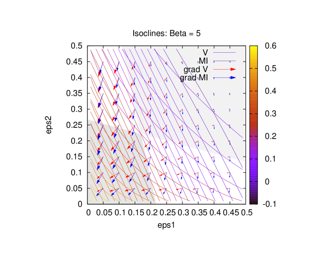
Figure 3: Isoclines of expected utility $V$ and mutual information $I(X;S)$ with corresponding gradient vectors showing the directions of steepest ascent (wrt/ the Fisher metric). The gray regions show which channels are more informative (dark gray) or less informative (light gray) than the channel with noise parameters $(\epsilon_{1}=0.17,\epsilon_{2}=0.22)$, in the sense of the term arising in Blackwell’s analysis.

5.2 Leader-follower example

Next, we turn to a simple games involving two players, namely a leader $A^{1}$ and a follower $A^{2}$ (see Fig. 4).

Figure 4: A 2-player game where player $A^{1}$ (leader) can move before player $A^{2}$ (follower).

In contrast to the single-player game, now the distribution $p(X)$ of the state of Nature is replaced by the equilibrium strategy $\sigma(a_{1})$ of player $1$, a strategy that will also depend on the parameters ${\boldsymbol{\theta}}$. Another difference is that there are now two utility functions, one for each player.

As in the decision problem, we consider binary state spaces and an asymmetric binary channel with parameters ${\boldsymbol{\theta}}=(\epsilon^{1},\epsilon^{2})$. We use the utility functions of the players analyzed in [5]

		follower
	$u_{1}$/$u_{2}$	$L$	$R$
leader	$L$	(5, 2)	(3, 1)
	$R$	(6, 3)	(4, 4)

Bagwell pointed out that in the pure strategy Nash equilibria the leader can only take advantage of moving first (by playing $L$), when the follower can observe his move perfectly (Stackelberg solution). As soon as the slightest amount on noise is added to the channel only the equilibrium of the simultaneous move game (both playing $R$, the Cournot solution) remains. Here we show that our differential analysis uncovers a much richer structure. In particular, we show there exist a QRE branch and parameters for the noise of the channel such that both players prefer more noise.

In the decision case, we used $I(X;S)$ to quantify the amount of information that is available to the (single) player. In the multi-player game setting, the corresponding quantity is $I(A_{1};S)$, and strongly depends on the move of the leader. As an illustration, consider a symmetric channel $p(s|a_{1})$ parametrized by the single value $\epsilon\equiv\epsilon^{1,2}$. Fig. 5 shows how the strategy of the leader depends on the channel noise and the rationality $\beta=\beta^{1,2}$ of the players.

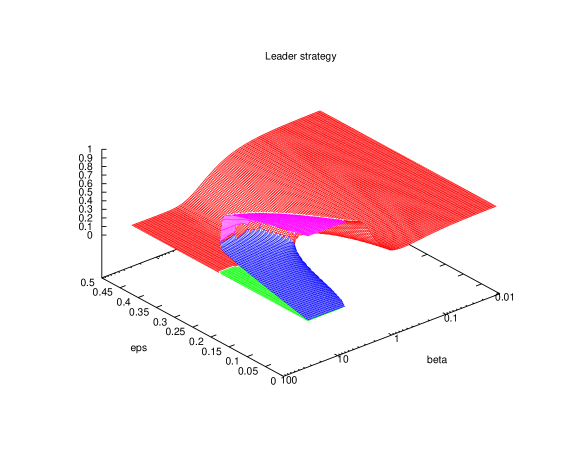
Figure 5: Surface of QRE equilibria for the symmetric channel leader-follower game.

This shows that for sufficiently rational players ($\beta>5$) there exist multiple QRE solutions. For $\beta\to\infty$ the three QRE equilibria converge to the pure strategy Nash equilibrium where both play $R$ (Cournot outcome, lower branch in red/green) and to the two mixed strategy Nash equilibria of the original game, respectively. For $\epsilon=0$, the upper mixed strategy equilibrium coincides with the equilibrium mentioned above where the leader has an advantage. In the following, we focus on the branch that smoothly connects to the origin $\beta=0$, the so-called “principal branch”, which includes that upper equilibrium.

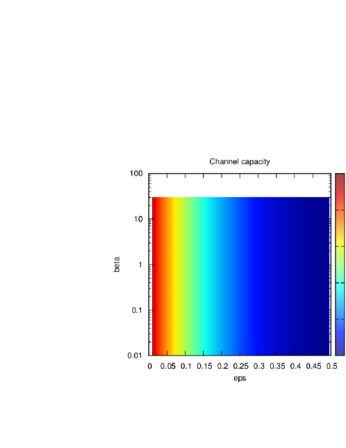
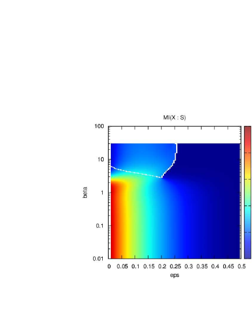
Figure 6: Channel capacity and mutual information $I(A_{1};S)$ in the symmetric channel leader-follower game.

Fig 6 shows the channel capacity as a function of the conditional distribution in the channel, as well as the mutual information $I(A_{1};S)$ that is actually transferred across the channel. As soon as the leader is rational enough, he starts to prefer the move $L$. This means that the mutual information $I(A_{1};S)$ decreases when the leader gets rational enough. However, the potential information that could be transferred, i.e., the channel capacity, is independent of player strategies, and so is still high. This illustrates how studying the information capacity rather than the mutual information is perhaps more in line with standard game theory, where the information partition is considered as part of the specification of the game parameters, independent of the resultant player strategies. For these reasons we focus our analysis on the channel capacity.

In this simple symmetric-channel scenario the space of game parameters concerning the channel noise is one-dimensional, and so analyses of “gradients” over that space are not particularly illuminating. Accordingly, to further investigate the role of information in the leader-follower game we consider an asymmetric channel, so that $p(s|a_{1})$ is parametrized by two noise parameters, $\epsilon^{1},\epsilon^{2}$, giving the probability of error for the two inputs $a_{1}=L$ and $a_{1}=R$ respectively. We also fix $\beta=10$ for both players. In this case, we again find multiple QRE branches when the channel noise is small enough. We focus on the branch where the leader has the biggest advantage and can achieve the highest utility while the utility of the follower is lowest. In the following, we refer to this QRE solution as the “Stackelberg branch”.

A)	B)

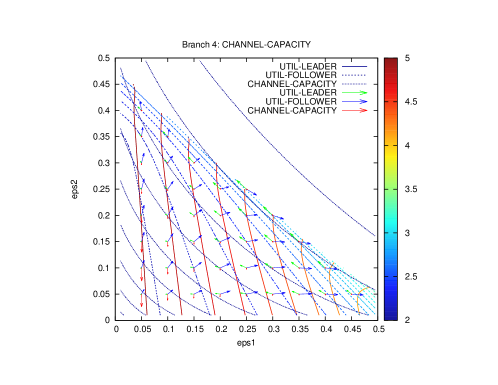
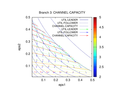
Figure 7: Isoclines of the expected utilities for the leader and the follower as well as the channel capacity in the asymmetric channel scenario, on the Stackelberg branch (A) and on the branch just below it in the space of leader strategies (B). The expected utility levels are color-coded and the channel capacity (dotted) increases towards the origin (lower-left corner). The gradient vectors show the corresponding directions of steepest ascent (wrt/ the Fisher metric).

Fig. 7 A shows the isoclines of expected utility for both leader and follower, the isoclines of the channel capacity, and the corresponding gradient fields, all on the Stackelberg branch. We immediately see that the gradients are nowhere collinear. So from Prop. 1 we know that for all values of the game parameters, the channel noises can be infinitesimally changed such that the capacity increases whereas the expected utility (of either the leader or follower) decreases. More interestingly, the gradient field shows that everywhere $\mathtt{grad}[\mbox{Capacity}]\notin Con(\{\mathtt{grad}(V)^{1},\mathtt{grad}V^{2}\})$. Thus by Prop. 4, there must be directions such that both players are better off and yet the channel capacity decreases when the game is moved in that direction. As before, while this is true locally, it does not mean that both players prefer less information globally.

Simply by redefining $f$ as the negative of the capacity as the function of interest (which amounts to flipping the corresponding gradient vectors in our figures), the same condition in Prop. 4 can be used to identify regions of channel parameter space where (there are directions in which we can move the game parameters in which) both players prefer more capacity. Now $\mathtt{grad}(-\mbox{Capacity})\in Con(\{\mathtt{grad}(V)^{1},\mathtt{grad}(V)^{2}\})$, except for a small region in the upper left corner (containing for example the point $(\epsilon^{1}=0.05,\epsilon^{2}=0.35)$). So we can immediately conclude that there are no such directions, for all parameter values outside this region.

To illustrate the effect of our choice of which equilibrium branch to analyze, Fig. 7 B shows the corresponding isoclines on the branch just below the Stackelberg branch. Again, the gradient vectors are nowhere aligned. However now $\mathtt{grad}[\mbox{Capacity}]$ $\in$ $Con(\{\mathtt{grad}(V)^{1},\mathtt{grad}V^{2}\})$. Thus, we can conclude that on this branch there are no directions where both players prefer a decrease in channel capacity, in contrast to the case on the Stackelberg branch.

Summarizing, even in rather simple leader-follower games, there is a surprisingly complicated underlying geometric structure. However just like in the decision-theoretic scenario, our theorems provide general conditions on the gradient vectors in leader-follower games that determine regions of channel parameter space in which there is negative value of information for both players. Moreover, these conditions are easily checked. In particular, they do not require laboriously comparing different information partitions to get non-numeric partial orders. Instead our conditions are based on cardinal quantifications of how much the players value infinitesimal changes to the information structure of the game, measured in units of utility per bits of information.

This kind of analysis can be applied multiple times at once, to quantify how much the players value different candidate changes to the information structure of the game. These quantifications are all measured in the same units, of utility per bits of information. So we can use their values to evaluate marginal rates of substitution of various kinds of changes to the game’s information structure. More generally, we can apply our analysis to quantify how much the players value different candidate infinitesimal changes to any aspects of the game specification, e.g., to parameters in utility functions. This allows us to evaluate marginal rates of substitution of all aspects of the game specification. This is the subject of future research.

5.3 Illustrative examples

To illustrate the generality of our framework, in this section we present additional examples, emphasizing the implications of our results in Sec. 4 for several different economic scenarios.

Example 1.

Consider a variant of the well-known scenario where a decision by an individual is a costly signal to a prospective employer of their capability as employees. In this variant there is a car repair chain that wants to hire a new mechanic. (So we have two players.) There is an applicant for the position who has some pre-existing ability at car repair. That ability is their type; it is determined by a prior distribution that neither player can affect. The repair chain cannot directly observe the applicant’s ability. So instead, they will give the applicant a written test of their knowledge of cars. The repair chain will then use the outcome of that test to decide whether to offer the job to the applicant and if so, at what salary. (The idea is that giving too low a salary to a new mechanic will raise the odds that after being trained by the repair chain that new mechanic would simply leave for a different repair chain, at a cost to the repair chain.)

The applicant will study before they take the test. The harder they study, the greater the cost to them. There is also a conditional distribution of how they do on the test given their ability to repair cars and how hard they study. The fact that that distribution is not a single-valued map means it is a noisy information channel, from the studying decision of the applicant to the outcome of the test.

Suppose that the repair chain feels frustrated by the fact that the test gives them a noisy signal of the applicant’s ability to repair cars. Knowing this, a test-design company approaches the repair chain, and offers to sell them a new test that has a double-your-money back guarantee that it is less noisy than the current test (for some functional of how “noisy” a test is that the test company and repair chain both use). Thinking they will get double their money back if they buy the new test but have lower expected utility, the repair chain buys the test.

Our results show that generically, there are ways that the repair chain will have lower expected utility with the new test — but not be able to invoke the guarantee to get any money back from the test-design company, since the new test is less noisy than the old one. That is, there are directions $\delta{\boldsymbol{\theta}}$ in the parameters describing how the test is designed, such that the test is made more accurate, but less useful for the repair chain, i.e. it has a negative value of information.

A	B

Figure 8: MAID for the noisy signalling game described in example 1 (panel A) and the leader-follower game from section 5 (panel B).

The MAID corresponding to this noisy signaling game is shown in Fig. 8 A. For comparison, panel B reproduces the MAID for the leader-follower game that was studied in section 5. In the noisy signaling game there is an additional Nature node $T$ which player 1 (the applicant) can observe, but that player 2 (the car repair chain) cannot observe. Another difference is that now the utility of both players depends in part on the outcome of Nature’s choice. Since the applicant incurs a cost if she studies, her utility directly depends on her move (study hard or party). However the utility of the repair chain does not depend directly on the move of the applicant.

We now present a variant of Braess’ paradox [10] which provides a particularly striking example of how extra information can simultaneously hurt all players of a game, even in the case of many players. Braess’ paradox is a “paradox” that arises in congestion games over networks. Although it has arisen in the real world in quite complicated transportation networks, it can be illustrated with a very simple network. We illustrate in this next example, before presenting our variant of Braess’ paradox.

Example 2.

Consider a scenario where there are 4000 players, all of whom must commute to work at the same time, from a node “Start” on a network to a node “End”. Say that there are a total of four roadways between Start and End that all the players know exist. (See Fig. 9.)

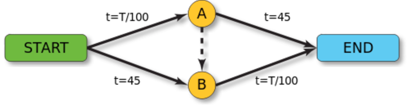
Figure 9: Network exhibiting Braess’ paradox. The symbols are explained in the text.

The move of each player is a choice of what route they will follow to get to work. There are two choices they can make. The first is the route Start-A-End, and the second is the route Start-B-End. The number of minutes it takes each player to follow their chosen route is illustrated in Fig. 9. In that figure, $t$ indicates the amount of time it takes a player to cross the associated road. In addition, $T$ refer to the total number of players (out of 4000) who follow the associated road. So on those two roads where $t=T/100$, the greater the amount of traffic $t$, the slower the players can drive, and so the greater the amount of time $T$ it takes to cross the road. In contrast, it takes 45 minutes to traverse the other two roads, regardless of the amount of traffic on the roads.

The paradox arises, if a new highway from A to B (dashed) is opened which takes only 4 minutes to traverse. Now, each player has a third option, namely to take the route Start-A-B-End. So we have a new game.

It is straightforward to verify that in all Nash equilibria of the original game, i.e. the game without the new highway, exactly half of the players choose Start-A-End, and half choose Start-B-End. The total cost (i.e., negative utility) to all players is a 65 minute commute. When the new highway is opened, every player will choose Start-A-B-End. This increases the travel time of all players to 84 minutes. Thus, the expected cost for all players rises when they have more possible actions.

Now consider a variant of Braess’ paradox where both games are changed slightly, so that they only differ in their information structures. In this variant, the new highway exists in both games, but is closed due to construction with prior probability of .1. We assume that the cost of 4 minutes is incurred by a player if they try to go down the new highway both if they are successful and get through to B, or if they are blocked by the new construction and have to return to A. In addition, in both games all players are informed about whether the new highway is open, but via a noisy signal (e.g. via a newspaper article from several days before saying when the new highway is schedule to open). The difference between the games is the amount of noise in that signal.

In the new first game, the signal is completely noisy, providing no information at all about whether the new highway is open. So the players have to decide their strategy based purely on the prior probability of .1 that the new highway is open. It is straightforward to verify that in this case, the Nash equilibrium is for half of the players to choose Start-A-End, half to choose Start-B-End, and none to try to go down the new highway. The resultant travel time per player is 65 minutes.

In contrast, in the new version of the second game, the signal is noise-free. So with probability .1 the new highway is open, all players know that, and therefore all take the new highway, for a total travel time of 84 minutes. With probability .9 the new highway is closed, all players know that, and therefore none try to take the new highway, for a total travel time of 65 minutes. So the expected travel time per player in the new second game is $.1(84)+.9(65)$.

So the extra information that is available in the new second game, but not in the new first game, hurts all players.

Note that in contrast to the leader-follower games and noisy signaling games analyzed above, in our variant of Braess’ paradox the extra information concerns a move of Nature, not the move of some other player. Nevertheless, our results on negative value of information still apply. In particular, for any particular player $i$ in that game, and any precise choice for information-theoretic function $f$, Prop. 1 tells us that there are other directions $\delta\boldsymbol{\theta}$ in which we infinitesimally reduce the noise in the signal about the state of the highway so that information increases and expected utility for player $i$ goes up. Prop. 3 then tell us that this property is generic, i.e., it is true for almost all utility functions that differ only slightly from the ones in Ex. 2.

This may have important real-world applications. Computer routing networks (e.g., networks that route communication packets, jobs, etc.), are typically run in a distributed fashion where each router adaptively modifies its behavior to try to optimize its own “utility function” based on noisy signals it receives concerning the state of the overall network. In addition to arising in human transportation traffic networks, Braess’ paradox often arises in such computer routing networks [29]. This has led to a large body of work on how to redesign the adaptive algorithms used by the routers to avoid the paradox and associated loss of expected utility  [32, 30]. Our analysis suggests that it should be possible to avoid Braess’ paradox — and indeed to increase the expected utility — without redesigning the routing algorithms, but instead changing the signals the routers receive concerning the state of the network.

6 Future work

In this paper we primarily used our geometric framework to analyze the relationship between changes in information and associated changes in expected utility. However the framework is far more broadly applicable. It can be used to analyze the relationship between expected utilities and any function $f(\boldsymbol{\theta})$ that depends on the parameters specifying the game. $f$ is not restricted to be an information-theoretic function.

As a particularly simple illustration of this breadth of the applicability of our framework, we can use it to analyze the relationship between expected utility and a function $f(\boldsymbol{\theta})$ that simply returns one of the components of $\boldsymbol{\theta}$. This analysis reveals what might be called scenarios with “negative value of utility”:

Example 3.

This example concerns a simultaneous move game of two players, who have two possible moves each. The bimatrix of the game is as follows:

	L	R
T	(1,4)	(4-$\theta$,1)
B	(2,2)	(3,3)

where $\theta\geq 0$ is a parameter adjusting the utility of the row player.

With $\theta<1$ this game has no pure strategy Nash equilibrium. The unique Nash equilibrium of this game is a mixed equilibrium with the row player playing top with $p_{T}=\frac{1}{4}$ and the column player playing left with $p_{L}=\frac{1-\theta}{2-\theta}=1-\frac{1}{2-\theta}$. Since the column player is indifferent between $L$ and $R$ at the equilibrium, the expected utility $V_{col}$ is $\frac{5}{2}$ independent of $\theta$. While the row player has an expected utility of $V_{row}=\frac{5-2\theta}{2-\theta}$.

Now, $\frac{\partial V_{row}}{\partial\theta}=\frac{1}{(2-\theta)^{2}}$ is strictly positive which means that the row player prefers $\theta$ too increase. At the same time, this reduces her utility for the outcome $T,R$ and thus, one could say that the row player has a negative value of utility.

As Ex. 3 illustrates, our framework allows us to quantify the value of any infinitesimal change in the change in any function $f(\boldsymbol{\theta})$ induced by by an infinitesimal change in the game parameter. Indeed, we can evaluate such a value even if the induced change in $f(\boldsymbol{\theta})$ is indirect, arising via the effect of the change in $\boldsymbol{\theta}$ on the player strategy profile that is mediated by the equilibrium concept (as in the leader-follower game from Sec. 5 and as in Ex. 2).

This breadth of quantities whose “value” can be evaluated using our framework allows us to analyze the trade-offs, inherent in a game, among multiple changes to the parameters specifying that game and/or functions of those parameters. These trade-offs can be used to calculate marginal rates of substitution, in which we compare the values assigned by a single player to different changes in the game parameter. Assuming transferrable utility, they can also be used to compare the values assigned by different players to the same change in the game parameter. Under that assumption they can even be used to compare the values assigned by different players to different changes in the game parameter. For example, with our framework we can quantify the relationship between the value to player $i$ of changes to the information capacity of one information channel in a game, and the value to a separate player $j\neq i$ of changes to $i$’s utility function in that game. Similarly, by considering the QRE rationality parameter $\beta$ as a component of the game parameter $\boldsymbol{\theta}$, we can study the value of rationality and its relations with values of other quantities. This allows us to do things like quantify the relationship between extra rationality by player $i$ and extra information available to that player. Colloquially, “$i$’s knowing this much more about certain utility-relevant quantities before they make their move is equivalent to their being this much smarter when they make that move”. Future work involves making a detailed investigation of these kinds of trade-offs.

Another issue we intend to investigate in future work is “second-order effects”. Changing the parameter of a game $\boldsymbol{\theta}$ infinitesimally can affect the value of every function $g:\boldsymbol{\theta}\in\Theta\rightarrow{\mathbb{R}}$, not just functions like expected utilities, mutual information, etc. In particular, this is true if $g$ is the differential value of some $f(\boldsymbol{\theta})$ evaluated at $\boldsymbol{\theta}^{\prime}$. Changing $\boldsymbol{\theta}$ will not just change the expected utility of player $i$ and what $f(\boldsymbol{\theta})$ is; it will also change the differential value to player $i$ of changes to $f$. As an example, changing the conditional distribution specifying one information channel in a game will in general change the differential value of a different information channel. In future work we hope to investigate these second order effects and whether they depend on “second-order” properties of the geometric structure of the game, like the Ricci curvature tensor of the Fisher metric.

Since in general games have multiple equilibria, it is often impossible to infinitesimally change the game parameter in way that is Pareto-optimal simultaneously for all equilibria. In other future work, we intend to investigate the generalizations of Prop. 4 that determine when such changes are possible.

Finally, our framework provides important new capabilities for policy making or mechanism design, by providing guidance to a regulator external to a game on how to modify the components of the game parameter vector that are under their control. As discussed above, in games with multiple equilibria — arguably the majority of real-world games of interest to a regulator — it makes sense for the regulator to determine which equilibrium the players have adopted for a current value of $\boldsymbol{\theta}$ simply by observing how the players are behaving. Using our framework, it may be possible for that regulator to gradually change $\boldsymbol{\theta}$ from that starting value, to move the equilibrium down the branch that has the current equilibrium, to where it intersects with another branch, and then guide the equilibrium along that second branch, back to the starting $\boldsymbol{\theta}$. In this way the regulator may be able to gradually change player behavior to go from a current equilibrium of a game specified by $\boldsymbol{\theta}$, to a different, Pareto-superior equilibrium for that same $\boldsymbol{\theta}$. In some situations, the regulator should even be able to design that trajectory through the space of game parameter vectors so that each infinitesimal change to $\boldsymbol{\theta}$ along that trajectory is Pareto-improving. (See [31] for an example of this kind of approach.)

7 Conclusion

In this paper we introduce a new framework to study the value of information in arbitrary noncooperative games. Our starting point is the well-established concept of marginal utility of a good in a decision problem. We present a very natural way to generalize this, to marginal utility to a player in a noncooperative game of an arbitrary function of a parameter specifying that game. Interestingly, this generalization forces us to introduce a metric over the space of game parameters. In this way we show that geometry is intrinsic to noncooperative game theory, with each game specifying its own associated Riemannian manifold.

In parallel with this analysis, we consider the issue of how best to quantify economically relevant aspects of the information structure in that game. We argue that mutual information is a natural way to do this, using very simple considerations grounded in economics. As we discuss, such a (cardinal) quantification of information also has several advantages over the partial orders commonly used in the past to investigate the role of information in games.

We then combine our two analyses into a unified framework. We do this by taking the “function of a parameter specifying a game” from the first analysis to be the mutual information that was motivated in our second analysis. This combination of our two analyses reveals how a game’s geometry governs the relation between changes to its information structure and changes to the expected utilities of the players.

We then use our framework to derive general conditions for the existence of negative value of information. In particular, we show that for almost any game, there are changes to the information structure of the game that both increase the information available to any particular player in that game and hurt that player. We then extend our analysis to characterize the set of games where there are such changes that simultaneously increase the information available to all players, while hurting all players. We illustrate our framework with computational analyses of a single-player decision scenario as well as a two player leader-follower game.

Finally, we note that our framework can by applied to analyze the effects of arbitrary changes to a game, not just changes to its information structure. As a particularly simple example, we construct a game that has “negative value of utility”, in which the expected value of a player’s utility $u$ increases when we change the game by applying a monotonically decreasing transformation to $u$. More generally, the breadth of applicability of our framework allows us to analyze marginal rates of substitution of different aspects of an information structure, of the utility functions of the players, or of any other parameters specifying the game the players are engaged in.

Acknowledgments

NB acknowledges support by the Klaus Tschira Stiftung. The research of JJ was supported by the ERC Advanced Investigator Grant FP7-267087. DHW acknowledges support of the Santa Fe Institute.

Appendix A Review of conic hulls

In our analysis below we shall work in some tangent space of a parameter manifold that is equipped with the Fisher metric $\langle.,.\rangle$. Now, whenever we have a scalar product on such a (finite dimensional) vector space, we can perform a linear transformation of that vector space to turn that scalar product into the standard Euclidean one. Thus, in our analysis below, we shall essentially be doing elementary Euclidean geometry, just in a different coordinate system. This will be reflected in the fact that simple graphical pictures and intuition can be used to understand many of our results.

We start by reviewing some simple linear algebra in Euclidean space, that is, ${\mathbb{R}}^{d}$ equipped with the Euclidean scalar product $\langle.,.\rangle$. For a nonzero vector $\boldsymbol{v}\in{\mathbb{R}}^{d}$, the hyperplane $H_{0}(\boldsymbol{v})=\{\boldsymbol{w}:\langle\boldsymbol{v},\boldsymbol{w}\rangle=0\}$ separates ${\mathbb{R}}^{d}$ into two halfspaces $H_{+}(\boldsymbol{v})\;(H_{-}(\boldsymbol{v})\;resp.)\equiv\{\boldsymbol{w}:\langle\boldsymbol{v},\boldsymbol{w}\rangle>0\;(<0\;resp.)\}$, and for two vectors $\boldsymbol{v}_{1},\boldsymbol{v}_{2}$ that are not positively collinear, the associated halfspaces overlap, e.g.,

$$H_{+}(\boldsymbol{v}_{1})\cap H_{-}(\boldsymbol{v}_{2})\neq\emptyset.$$ (24)

When we have several nonzero vectors $\boldsymbol{v}_{i}$, their conic hull [9] is defined as

$$Con(\{\boldsymbol{v}_{i}\})\equiv\left\{\sum_{i}\alpha^{i}\boldsymbol{v}_{i}:\alpha_{i}\geq 0\forall i\right\}$$ (25)

Note that $C=Con(\{\boldsymbol{v}_{i}\})$ is a cone since whenever $\boldsymbol{v}\in C$, it follows that $k\boldsymbol{v}\in C$ for $k>0$. Note also that this cone is convex because whenever $\boldsymbol{v},\boldsymbol{w}\in C$, then $\lambda\boldsymbol{v}+(1-\lambda)\boldsymbol{w}\in C$ for $0\leq\lambda\leq 1$.

A cone $C$ is called pointed if it does not contain any bi-infinite straight line. The following will be used in the sequel:

Lemma 5.

If the vectors $\boldsymbol{v}_{i}$ are linearly independent, then $Con(\{\boldsymbol{v}_{i}\})$ is pointed.

Of course, the converse of Lemma 5 does not hold in general, because for all $\boldsymbol{v}\in Con(\{\boldsymbol{v}_{i}\})$, $Con(\{\boldsymbol{v}_{i}\})=Con(\{\boldsymbol{v}_{i}\}\cup\boldsymbol{v})$.

We will also need to use the definition that the dual to a conic hull $Con(\{\boldsymbol{v}_{i}\})$ is

$$Con(\{\boldsymbol{v}_{i}\})^{\bot}\equiv\bigcap_{i}H_{-}(\boldsymbol{v}_{i}).$$ (26)

Equivalently,

$$Con(\{\boldsymbol{v}_{i}\})^{\bot}=\{\boldsymbol{v}:\langle\boldsymbol{v},\boldsymbol{v}_{i}\rangle<0\text{ for all }i\}.$$ (27)

The following elementary property relating conic hulls and pointedness is used in the sequel.

Lemma 6.

$Con(\{\boldsymbol{v}_{i}\})$ is not pointed $\Rightarrow$ $[Con(\{\boldsymbol{v}_{i}\})]^{\bot}=\varnothing$ $\Rightarrow$ the vectors $\boldsymbol{v}_{i}$ are linearly dependent.

For any single vector $\boldsymbol{v}$, $Con(\boldsymbol{v})^{\bot}=H_{-}(\boldsymbol{v})$. In general, when we enlarge the set of vectors $\boldsymbol{v}_{i}$, $Con(\{\boldsymbol{v}_{i}\})$ gets larger whereas the dual conic hull $Con(\{\boldsymbol{v}_{i}\})^{\bot}$ becomes smaller. More precisely,

Lemma 7.

Let $C,C_{1},C_{2}$ be nonempty convex cones whose duals are nonempty. Then

$$C^{\bot\bot}=C$$ (28)

and

$$C_{1}\subset C_{2}\quad\Leftrightarrow\quad C_{2}^{\bot}\subset C_{1}^{\bot}.$$ (29)

The requirement that the duals be non-empty is crucial in this result. For example, if the second part of Lemma 29 held for empty $C^{\bot}$, then we would have $C^{\bot}=\varnothing\Rightarrow C^{\prime}\subset C$ for any conic hull $C^{\prime}\subseteq{\mathbb{R}}^{n}$. The only way this could be would be if $C={\mathbb{R}}^{n}$. However for any vector $\boldsymbol{v}\in{\mathbb{R}}^{n}$ with $n>2$, $[Con(\{\boldsymbol{v},-\boldsymbol{v}\})]^{\bot}=\varnothing$, even though $[Con(\{\boldsymbol{v},-\boldsymbol{v}\})]\neq{\mathbb{R}}^{n}$.

Appendix B Partial derivatives of QREs of MAIDs with respect to game parameters

For computations involving the partial derivatives of the players strategies at a QRE (branch) it can help to explicitly introduce the normalization constants as an auxiliary variable. The QRE condition from eq. (8) is then replaced by the following conditions

$$\sigma_{i}(a_{v}|x_{pa(v)};\beta_{i},\boldsymbol{\theta})-\frac{e^{\beta_{i}{\mathbb{E}}(u_{i}|a_{v},x_{pa(v)};\boldsymbol{\beta},\boldsymbol{\theta})}}{Z_{i}(x_{pa(v)};\beta_{i},\boldsymbol{\theta})} = 0$$

$$Z_{i}(x_{pa(v)};\beta_{i},\boldsymbol{\theta})-\sum_{a\in\mathcal{X}_{v}}{e^{\beta_{i}{\mathbb{E}}(u_{i}|a_{v},x_{pa(v)};\boldsymbol{\beta},\boldsymbol{\theta})}} = 0$$

for all players $i$, decision nodes $v\in\mathcal{D}_{i}$ and all states $a_{v}\in\mathcal{X}_{v},x_{v}\in\prod_{u\in Pa(v)}\mathcal{X}_{u}$. (Here and throughout this section, subscripts on $\sigma$, $Z$, etc. should not be understood as specifications of coordinates as in the Einstein summation convention.)

Overall, this gives rise to a total of $M$ equations for $M$ unknown quantities $\sigma_{i}(a_{v}|x_{pa(v)})$, $Z_{i}(x_{pa(v)})$. Using a vector valued function $\boldsymbol{f}$ we can abbreviate the above by the following equation:

$$\boldsymbol{f}(\boldsymbol{\sigma}_{\boldsymbol{\beta},\boldsymbol{\theta}},\boldsymbol{Z}_{\boldsymbol{\beta},\boldsymbol{\theta}},\boldsymbol{\beta},\boldsymbol{\theta})=\boldsymbol{0}$$ (30)

where $\boldsymbol{\sigma}_{\boldsymbol{\beta},\boldsymbol{\theta}}$ is a vector of all strategies

$$\{\sigma_{i}(a_{v}\mid x_{v};\beta_{i},\boldsymbol{\theta}):i=1,\ldots,n,v\in\mathcal{D}_{i},a_{v}\in\mathcal{X}_{v},x_{v}\in\prod_{u\in Pa(v)}\mathcal{X}_{u}\},$$

$\boldsymbol{Z}_{\boldsymbol{\beta},\boldsymbol{\theta}}$ collects all normalization constants, and $\boldsymbol{0}$ is the vector of all 0’s. Note that in general, even once the distributions at all decision nodes have been fixed, the distributions at chance nodes affect the value of ${\mathbb{E}}(u_{i}\mid a_{v},x_{pa(v)};\boldsymbol{\beta},\boldsymbol{\theta})$. Therefore they affect the value of the function $\boldsymbol{f}$. This is why $\boldsymbol{f}$ can depend explicitly on $\boldsymbol{\theta}$, as well as depend directly on $\boldsymbol{\beta}$.

The (vector-valued) partial derivative of the position of the QRE in $(\boldsymbol{\sigma}_{\boldsymbol{\theta}},\boldsymbol{Z}_{\boldsymbol{\theta}})$ with respect to $\boldsymbol{\theta}$ is then given by implicit differentiation of eq. (30) :

$$\left[\begin{array}[]{c}\frac{\partial\boldsymbol{\sigma}_{\boldsymbol{\theta}}}{\partial\boldsymbol{\theta}}\\ \frac{\partial\boldsymbol{Z}_{\boldsymbol{\theta}}}{\partial\boldsymbol{\theta}}\end{array}\right]=-\left[\frac{\partial\boldsymbol{f}}{\partial\boldsymbol{\sigma}_{\boldsymbol{\theta}}}\quad\frac{\partial\boldsymbol{f}}{\partial\boldsymbol{Z}_{\boldsymbol{\theta}}}\right]^{-1}\frac{\partial\boldsymbol{f}}{\partial\boldsymbol{\theta}}$$ (31)

where the dependence on $\boldsymbol{\beta}$ is hidden for clarity, all partial derivatives are evaluated at the QRE, and we assume that the matrix $\left[\frac{\partial\boldsymbol{f}}{\partial\boldsymbol{\sigma}_{\boldsymbol{\theta}}}\quad\frac{\partial\boldsymbol{f}}{\partial\boldsymbol{Z}_{\boldsymbol{\theta}}}\right]$ is invertible at the point $\boldsymbol{\theta}$ at which we are evaluating the partial derivatives.

These equations give the partial derivatives of the mixed strategy profile. They apply to any MAID, and allow us to write the partial derivatives of other quantities of interest. In particular, the partial derivative of the expected utility of any player $i$ is

$$\frac{\partial V_{i}}{\partial\boldsymbol{\theta}}=\sum_{x\in\mathcal{X}_{\mathcal{V}}}u_{i}(x)\frac{\partial p(x;\boldsymbol{\theta})}{\partial\boldsymbol{\theta}}=\sum_{x\in\mathcal{X}_{\mathcal{V}}}u_{i}(x)\sum_{v\in\mathcal{V}}\frac{\partial p(x_{v}\mid x_{pa(v)};\boldsymbol{\theta})}{\partial\boldsymbol{\theta}}\prod_{v^{\prime}\neq v}p(x_{v^{\prime}}\mid x_{pa(v^{\prime})};\boldsymbol{\theta})$$ (32)

where each term $\frac{\partial p(x_{v}\mid x_{pa(v)};\boldsymbol{\theta})}{\partial\boldsymbol{\theta}}$ is given by the appropriate component of Eq. (31) if $v$ is a decision node. (For the other, chance nodes, $\frac{\partial p(x_{v}\mid x_{pa(v)};\boldsymbol{\theta})}{\partial\boldsymbol{\theta}}$ can be calculated directly). Similarly, the partial derivatives of other functions of interest such as mutual informations between certain nodes of the MAID can be calculated from Eq. (31).

Evaluating those derivatives and the additional ones needed for the Fisher metric by hand can be very tedious, even for small games. Here, we used automatic differentiation [27] to obtain numerical results for certain parameter settings and equilibrium branches. Note that automatic differentiation is not a numerical approximation, like finite differences or the adjoint method. Rather it uses the chain rule to evaluate the derivative alongside the value of the function.

References

- [1]
- Amblard, Michel, and Morfu [2005] Amblard, P.-O., O. J. J. Michel, and S. Morfu (2005): “Revisiting the asymmetric binary channel: joint noise-enhanced detection and information transmission through threshold devices,” Proc. SPIE, 5845, 50–60.
- Arrow [1971] Arrow, K. J. (1971): “The value of and demand for information.,” in Decision and Organization, ed. by C. B. McGuire, and R. Radner, pp. 131–139. North-Holland, Amsterdam.
- Backhaus, Bent, Bono, Lee, B., D.H., and Xie [in press] Backhaus, S., R. Bent, J. Bono, R. Lee, T. B., W. D.H., and D. Xie (in press): “Cyber-Physical Security: A Game Theory Model of Humans Interacting over Control Systems,” IEEE Trans. on smart grids.
- Bagwell [1995] Bagwell, K. (1995): “Commitment and observability in games,” Games and Economic Behavior, 8, 271–280.
- Bergemann and Morris [2013] Bergemann, D., and S. Morris (2013): “The Comparison of Information Structures in Games: Bayes Correlated Equilibrium and Individual Sufficiency,” Discussion paper, SSRN, Economic Theory Center Working Paper No. 054-2013.
- Blackwell [1953] Blackwell, D. (1953): “Equivalent comparisons of experiments,” The Annals of Mathematical Statistics, 24(2), 265–272.
- Bono and Wolpert [2014] Bono, J. W., and D. H. Wolpert (2014): “Game Mining: How to Make Money from those about to Play a Game Game Mining: How to Make Money from those about to Play a Game Game Mining: How to Make Money from those about to Play a Game,” Advances in Austrian Economics.
- Boyd and Vandenberghe [2003] Boyd, S., and L. Vandenberghe (2003): Convex Optimization. Cambridge University Press.
- Braess [1968] Braess, D. (1968): “Über ein Paradoxon aus der Verkehrsplanung,” Unternehmensforschung, 12(1), 258–268.
- Cover and Thomas [1991] Cover, T., and J. Thomas (1991): Elements of Information Theory. Wiley-Interscience, New York.
- Doshi, Zeng, and Chen [2009] Doshi, P., Y. Zeng, and Q. Chen (2009): “Graphical models for interactive POMDPs: representations and solutions,” Autonomous Agents and Multi-Agent Systems, 18(3), 376–416.
- Gossner [2000] Gossner, O. (2000): “Comparison of Information Structures,” Games and Economic Behavior, 30, 44–63.
- Gossner [2010] (2010): “Ability and knowledge,” Games and Economic Behavior, 69(1), 95–106.
- Howard and Matheson [2005] Howard, R. A., and J. E. Matheson (2005): “Influence diagram retrospective,” Decision Analysis, 2(3), 144–147.
- Jost [6th edition, 2011] Jost, J. (6th edition, 2011): Riemannian geometry and geometric analysis. Springer.
- Kelly [1956] Kelly, J. L. (1956): “A new interpretation of information rate,” Information Theory, IRE Transactions on, 2(3), 185 –189.
- Koller and Friedman [2009] Koller, D., and N. Friedman (2009): Probabilistic Graphical Models. MIT Press.
- Koller and Milch [2003] Koller, D., and B. Milch (2003): “Multi-agent influence diagrams for representing and solving games,” Games and Economic Behavior, 45, 181–221.
- Lee, Wolpert, Backhaus, Bent, Bono, and B. [2013] Lee, R., D. Wolpert, S. Backhaus, R. Bent, J. Bono, and T. B. (2013): “Counter-Factual Reinforcement Learning: How to Model Decision-Makers That Anticipate the Future,” in Decision-Making with Imperfection, ed. by M. K. T. Guy, and D.H.Wolpert. Springer.
- Lee, Wolpert, Backhaus, Bent, Bono, and Tracey [2012] Lee, R., D. Wolpert, S. Backhaus, R. Bent, J. Bono, and B. Tracey (2012): “Predicting What Reinforcement Learning Will Tell You: A Model of Human Decision-Making in Multi-Stage Games,” in Decision-Making with Imperfect Decision Makers 2012. springer.