Higgs as a Probe of Supersymmetric Grand Unification with the Hosotani Mechanism

Abstract

The supersymmetric grand unified theory where the $SU(5)$ gauge symmetry is broken by the Hosotani mechanism predicts the existence of adjoint chiral superfields whose masses are at the supersymmetry breaking scale. The Higgs sector is extended with the $SU(2)_{L}$ triplet with hypercharge zero and neutral singlet chiral multiplets from that in the minimal supersymmetric standard model. Since the triplet and singlet chiral multiplets originate from a higher-dimensional vector multiplet, this model is highly predictive. Properties of the particles in the Higgs sector are characteristic and can be different from those in the Standard Model and other models. We evaluate deviations in coupling constants of the standard model-like Higgs boson and the mass spectrum of the additional Higgs bosons. We find that our model is discriminative from the others by precision measurements of these coupling constants and masses of the additional Higgs bosons. This model can be a good example of grand unification that is testable at future collider experiments such as the luminosity up-graded Large Hadron Collider and future electron-positron colliders.

I Introduction

One of the most prominent achievements in particle physics in the past decades is discovery of a new boson whose mass is around 125 GeV, as reported in 2012 by the ATLAS and CMS collaborations of the CERN Large Hadron Collider (LHC) LHC . After that, properties of the new particle have been carefully investigated, and turned out to be consistent with those of the Standard Model (SM) Higgs boson. Now the SM has been established as a successful low energy effective theory that can consistently describe phenomena below the energy scale of ${\cal O}(100)$ GeV.

However, several high energy experiments and cosmological observations show evidences for new physics beyond the SM, which include neutrino oscillations, existence of dark matter and baryon asymmetry of the universe. In addition to such experimental results, the SM suffers from theoretical problems. One is a serious fine-tuning problem called the hierarchy problem. To reproduce the weak scale Higgs boson mass, huge cancellation between its bare mass and contribution from radiative corrections is required. Another is that the reason why the electric charges of the SM particles are fractionally quantized is unexplained.

It is intriguing that some of theoretical problems can be elegantly solved by introducing concepts of supersymmetry (SUSY) and grand unification GUT ; SUSY-GUT . The SUSY offers us a solution to the hierarchy problem. The quadratically divergent contributions to the Higgs boson mass from the SM particles are canceled if we introduce their partner particles whose spins differ from those of the corresponding SM particles by half. Grand Unified Theories (GUTs) provide unified descriptions of the SM gauge groups. Simultaneously, SM fermion multiples are embedded into larger group representations, leading to the charge quantization. Therefore, combination of the SUSY and the grand unification is an excellent candidate for the underlying theory. Moreover, in the minimal SUSY GUT, the three gauge coupling constants are naturally unified at a high energy scale.

Although the idea itself is fascinating, GUT models have several difficulties. Notice that the typical energy scale of the gauge coupling unification (GCU) in conventional SUSY GUTs is around $10^{16}$ GeV. Given such a high GUT scale, superheavy GUT particles completely decouple from the low energy effective theory Appelquist:1974tg . Therefore, testing GUTs usually relies on checking relations among masses and coupling constants at the TeV scale, which are related to each other through renormalization group equations (RGEs). Moreover, there is a fine tuning problem about the mass splitting between the electroweak Higgs doublets and colored Higgs triplets, and many ideas to solve the doublet-triplet (DT) splitting have been proposed DW ; SlidingSinglet ; missingPARTN ; pNG ; orbifoldGUTs ; Kakizaki:2001en . In extended SUSY GUT models, the successful GCU is spoiled in many cases and the GCU becomes a constraint instead of a prediction.

Recently, a SUSY GUT model that circumvents the above mentioned difficulties is proposed by one of the authors gGHU-DTS by supersymmetrizing the Grand Gauge-Higgs Unification (GHU) gGHU , where the GCU is just a constraint as in many extended SUSY GUT models. We call the supersymmetric version the Supersymmetric Grand Gauge-Higgs Unification (SGGHU) in this paper. The idea of the Grand GHU is to break the GUT gauge group by applying the so-called Hosotani mechanism hosotani . In the SGGHU, by using non-trivial vacuum expectation value (VEV) of a Wilson loop, the doublet-triplet splitting problem is naturally solved. As a by-product, existence of new light chiral adjoints is predicted. At the TeV scale, our model is reduced to the Minimal Supersymmetric Standard Model (MSSM) with a color octet superfield, an $SU(2)_{L}$ triplet superfield with hypercharge zero and a neutral singlet superfield. In particular, since the Higgs sector is extended by the triplet and singlet superfields, we can test our GUT model by exploring properties of the extended Higgs sector with collider experiments. Due to couplings between the MSSM Higgs doublets and the new Higgs triplet and singlet, the SM-like Higgs boson mass can be more naturally as large as 125 GeV, as compared to the prediction of the MSSM MSSMHiggsMass ; MSSMHiggsMass2 . Thus, the little hierarchy can also be relaxed. As we see later, even when the masses of the triplet and singlet superfields are as small as the electroweak scale, it turns out that the mass of the color octet is too large to probe its effects at colliders due to radiative effects.

In this paper, we focus on the Higgs sector of the SGGHU, and explore its phenomenological consequences. We derive values of parameters in the low energy effective theory using the RGEs, and evaluate how the masses and couplings of the SGGHU Higgs sector particles are modified from those in the MSSM due to the existence of the light triplet and singlet chiral multiplets. We emphasize that by measuring the masses and couplings of the Higgs bosons precisely at the LHC and future electron-positron colliders such as the International Linear Collider (ILC) ILC and the CLIC CLIC , particle physics models can be distinguished. We show that the SGGHU is a good example to show the capabilities of collider experiments for testing GUT scale physics.

This paper is organized as follows. In Sec. II, we briefly review the model of the SGGHU and its low energy effective theory. Particular attention is paid to the Higgs sector, which is extended by the triplet and singlet chiral multiplets. Sec. III is devoted to the discussion of the SM-like Higgs boson mass using RGEs. Some benchmark points reproducing the observed Higgs boson mass are provided. In Sec. IV, predictions about couplings of the SM-like Higgs boson and mass relation of additional Higgs bosons are presented based on the benchmark points. Definitions of model parameters and RGEs are collected in Appendix A. Mass matrices of Higgs bosons, neutralinos and charginos are summarized in Appendix B. Necessary formulae for computing radiative corrections to the SM-like Higgs boson mass are also given there.

II Model

II.1 Review of Supersymmetric Grand Gauge-Higgs Unification

In this subsection, we briefly review the grand GHU scenario proposed in Ref. gGHU-DTS . This scenario is a kind of the grand unification where the Hosotani mechanism hosotani is employed to break the $SU(5)$ unified gauge symmetry. The simplest setup that can accommodate the chiral fermions is a five-dimensional (5D) $SU(5)$ model compactified on an $S^{1}/{\mathbb{Z}}_{2}$ orbifold with its radius being of the GUT scale. We first discuss the non-SUSY version of the simplest setup discussed in Ref. gGHU for illustration purpose, and then supersymmetrize it gGHU-DTS .

The Hosotani mechanism is a mechanism for gauge symmetry breaking which works on higher-dimensional gauge theories. To be more concrete, the zero modes of extra-dimensional components of the gauge fields, which behave as scalar fields after the compactification, develop VEVs to break the gauge symmetry. In order to apply this mechanism to the $SU(5)$ unified gauge symmetry breaking, massless adjoint scalar fields, with respect to the $SU(5)$ symmetry that remains unbroken against the boundary conditions (BCs), should appear. It is known that such components tend to be projected out in models that realize the chiral fermions due to the orbifold BCs. In Ref. gGHU , this difficulty is evaded via the so-called diagonal embedding method DiagonalEmbedding which is proposed in the context of the string theory. In our field theoretical setup on the $S^{1}/{\mathbb{Z}}_{2}$ orbifold, we impose two copies of the gauge symmetry with an additional discrete symmetry that exchanges the two gauge symmetries. Namely, the symmetry is $SU(5)\times SU(5)\times{\mathbb{Z}}_{2}$ in our $SU(5)$ model. Here, we name the gauge fields for the two $SU(5)$ groups $A^{(1)}_{M}$ and $A^{(2)}_{M}$, respectively, where $M=\mu(=0\mbox{-}3),5$ is a 5D Lorentzian index, and define the eigenstates of the ${\mathbb{Z}}_{2}$ action as $X^{(\pm)}=(X^{(1)}\pm X^{(2)})/\sqrt{2}$. We set the BCs around the two endpoints of the $S^{1}/{\mathbb{Z}}_{2}$, $y_{0}=0$ and $y_{\pi}=\pi R$, as

$$A_{\mu}^{(1)}(y_{i}-y)=A_{\mu}^{(2)}(y_{i}+y),\qquad A_{5}^{(1)}(y_{i}-y)=-A_{5}^{(2)}(y_{i}+y),$$ (1)

for $i=0,\pi$, where $y$ denotes the 5th dimensional coordinate. With these BCs, we see that $A_{\mu}^{(+)}$ and $A_{5}^{(-)}$ obey the Neumann BC at each endpoint to have the zero-modes, and thus that the gauge symmetry remaining unbroken in the 4D effective theory is the diagonal part of the $SU(5)\times SU(5)$ (or our GUT symmetry is embedded into the diagonal part) and an adjoint scalar field is actually realized.

An interesting point is that the $A_{5}^{(-)}$ is not a simple adjoint scalar field but composes a Wilson loop since it is a part of the gauge field. The Wilson loop is given by

$$W={\cal P}\exp\left(i\int_{0}^{2\pi R}\frac{g}{\sqrt{2}}{{A_{5}^{(-)}}^{a}(T_{1}^{a}-T_{2}^{a})}dy\right)\to\exp\left(i{\rm diag}\left(\theta_{1},\theta_{2},\theta_{3},\theta_{4},\theta_{5}\right)\right),$$ (2)

where ${\cal P}$ denotes the path-ordered integral, $g$ is the common gauge coupling constant, $T_{1}$ and $T_{2}$ are the generators of the two $SU(5)$ symmetries, and $a$ is an $SU(5)$ adjoint index. In the last expression, we show the expression on the fundamental representation for concreteness, and we have used the (remaining) $SU(5)$ rotation to diagonalize $A_{5}^{(-)}$. This expression shows that the VEV (and actually the system itself) is invariant under the shift $\theta_{i}\to\theta_{i}+2\pi$.

The form of the VEV which is discussed in Ref. gGHU and which we are interested in is given by $\theta_{1}=\theta_{2}=\theta_{3}=2\pi$ and $\theta_{4}=\theta_{5}=-3\pi$, i.e. $\left\langle W\right\rangle={\rm diag}(1,1,1,-1,-1)\equiv P_{W}$. This VEV does not affect the triplet component of the ${\bf 5}$ representation but does affect the doublet to split them. This “missing VEV”, which is forbidden for a simple adjoint scalar field by the traceless condition, is allowed since the Wilson loop is valued on a group instead of an algebra and thus is free from the condition. This fact plays an essential role to solve the DT splitting problem.

In this paper, for simplicity, we do not consider matter fields that are non-singlet under the both gauge groups. We introduce for instance a fermion $\Psi({\bf R},{\bf 1})^{(1)}$ with ${\bf R}$ being a representation of the $SU(5)$ group and its ${\mathbb{Z}}_{2}$ partner $\Psi({\bf 1},{\bf R})^{(2)}$. Here, we call the above pair a ”bulk ${\bf R}$ multiplet”. Their BCs are given as $\Psi^{(1)}(y_{\pi}-y)=-\eta_{i}^{\Psi}\gamma_{5}\Psi^{(2)}(y_{\pi}+y)$ where $\eta_{i}=\pm 1$ is a parameter associated with each fermion. As one of $\eta_{i}$ can be reabsorbed by changing $\gamma_{5}$, i.e. by the charge conjugation, we set $\eta_{0}=+1$ and $\eta_{\pi}=\eta$ hereafter. Then, $\Psi_{L}^{(+)}$ and $\Psi_{R}^{(-)}$ have the zero-modes when $\eta=+1$ while they do not when $\eta=-1$, when the VEV of $A_{5}$ vanishes.

Notice that it is always possible to gauge away the VEV of $A_{5}$ ($\propto\theta$). In this basis, called the Scherk-Schwartz basis, the $SU(5)$ breaking effect appears only on the BCs as

$$\Psi^{(1)}(y_{\pi}-y)=-\eta_{i}^{\Psi}\gamma_{5}W_{\bf R}\Psi^{(2)}(y_{\pi}+y),$$ (3)

where $W_{\bf R}$ is the Wilson line phase acting on ${\bf R}$. In concrete, for ${\bf R}={\bf 5}$ with $\eta=-1$ when the above VEV $\left\langle W\right\rangle=P_{W}$ is realized, the doublet component has the zero-mode while the triplet does not.

The same story as discussed above can be applied also to the SUSY extensions if we replace all the fields by the corresponding superfields. Thus, once the desired VEV $P_{W}$ is obtained, the DT splitting is easily realized by introducing a bulk ${\bf 5}$ hypermultiplet with $\eta=-1$ for the MSSM Higgs fields. In a similar way, if we introduce bulk ${\bf 10}$ hypermultiplets with $\eta=+1$, light vector-like pairs $(U,\bar{U})$ ($(\bar{\bf 3},{\bf 1})_{-2/3}$) and $(E,\bar{E})$ ($({\bf 1},{\bf 1})_{1}$) appear, where the values denote $SU(3)_{C},SU(2)_{L}$ and $U(1)_{Y}$ quantum numbers. This is utilized to recover the gauge coupling unification later.

We note that the zero-modes appear always in vector-like pairs from the bulk fields. The chiral fermions can be put simply on each boundary. Interestingly, when the VEV $\left\langle W\right\rangle=P_{W}$ is realized, bulk fields serve vector-like pairs in $SU(5)$ incomplete multiplets while the boundary fields which do not couple to $A_{5}$ and thus neither to the $SU(5)$ breaking do chiral fermions in $SU(5)$ full multiplets.

The remaining task to show that the DT splitting problem is actually solved is to examine when the VEV is realized. Here, we do not request that the vacuum resides on the global minimum but just require only that it is stable so that the lifetime is long enough. For this purpose, we have to check if there is no huge tadpole term for the fluctuation of $\theta_{i}$ around the desired vacuum, $\delta\theta_{i}$, and if it is not tachyonic around the desired vacuum. Since there are two largely different scales, the compactification scale and the SUSY breaking scale, the RG analysis should be performed.

Before going on the low energy effective theory, we note that the exchanging ${\mathbb{Z}}_{2}$ symmetry, under which $\delta\theta_{i}$ is odd, remains unbroken on the relevant vacuum even though $\theta_{i}$ is non-trivial. This is understood by the transformation of the Wilson line which is the order parameter. Under the ${\mathbb{Z}}_{2}$ action $W$ transforms as $W\to W^{*}$ and the VEV $\left\langle W\right\rangle$ is invariant since it is real. This ${\mathbb{Z}}_{2}$ invariance prohibit the tadpole terms. In the following, we introduce soft ${\mathbb{Z}}_{2}$ breaking as small as the SUSY breaking scale, and thus a small tadpole term will be generated.

II.2 Low Energy Effective Theory

As a consequence of the supersymmetrization of the grand gauge-Higgs unification, there appear adjoint chiral superfields whose gauge quantum numbers are the same as the SM gauge bosons. Since these new adjoint fields are originally embedded in the five-dimensional vector multiplets, their masses vanish in the SUSY limit. The chiral adjoints acquire masses after the SUSY breaking. Therefore, typical masses of the adjoint supermultiplets are of the order of the SUSY breaking scale irrelevantly to the compactification scale.

The low energy effective theory contains $SU(3)_{C}$ octet, $SU(2)_{L}$ triplet and singlet chiral superfields in addition to the MSSM superfields. As discussed later, since the mass of the octet chiral superfield is $O(10)$ TeV due to the radiative correction, its effect on the TeV scale phenomenology is negligible. Therefore, we here focus on the impact of the Higgs sector with the $SU(2)_{L}$ triplet and singlet chiral superfields.

The Higgs sector is composed of the superfields shown in Tab. 1. Here, $H_{u}$ ($H_{d}$) gives masses to the up-type quarks (down-type quarks and charged leptons). The superpotential of the effective theory of our model is given by

$$W=\mu H_{u}\cdot H_{d}+\mu_{\Delta}{\rm tr}(\Delta^{2})+\frac{\mu_{S}}{2}S^{2}+\lambda_{\Delta}H_{u}\cdot\Delta H_{d}+\lambda_{S}SH_{u}\cdot H_{d}\,,$$ (4)

where $\Delta=\Delta^{a}\sigma^{a}/2$ with $\sigma^{a}(a=1,2,3)$ being the Pauli matrices. Notice that there are no trilinear self-couplings among $S$ and $\Delta$ although such couplings are not prohibited by the symmetry of the effective theory because $S$ and $\Delta$ originate from the gauge supermultiplet. Moreover, the two new Higgs couplings $\lambda_{\Delta}$ and $\lambda_{S}$ are unified with the unified gauge coupling $g_{\rm GUT}$ as $\lambda_{\Delta}=2\sqrt{5/3}\lambda_{S}=g_{\rm GUT}$ at the GUT scale. Thus, this model is predictive up to the soft SUSY breaking parameters. Masses of the fermionic components of $S$ and $\Delta$ are denoted by $\mu_{S}$ and $\mu_{\Delta}$, respectively, and their magnitudes are of the order of the TeV scale because they are generated due to the SUSY breaking Burdman:2002se . Similarly, the supersymmetric tadpole parameter of $S$ is expected to be of the order of $\mu m_{\rm SUSY}$, as discussed in the previous section. This tadpole term is removed by field redefinition without loss of generality. The soft SUSY breaking terms are written by

$$V_{\rm soft} = \widetilde{m}_{H_{d}}^{2}|H_{d}|^{2}+\widetilde{m}_{H_{u}}^{2}|H_{u}|^{2}+2\widetilde{m}_{\Delta}^{2}{\rm tr}(\Delta^{\dagger}\Delta)+\widetilde{m}_{S}^{2}|S|^{2}$$ (5)

$$+\left[B\mu H_{u}\cdot H_{d}+\xi S+B_{\Delta}\mu_{\Delta}{\rm tr}(\Delta^{2})+\frac{1}{2}B_{S}\mu_{S}S^{2}\right.$$

$$\hskip 15.00002pt\left.+\lambda_{\Delta}A_{\Delta}H_{u}\cdot\Delta H_{d}+\lambda_{S}A_{S}SH_{u}\cdot H_{d}+{\rm h.c.}\phantom{\frac{1}{2}}\right].$$

The low energy values of these parameters introduced in the Higgs sector are obtained by solving the RGEs, which are discussed in the next section. It should be also noted that the VEV of the neutral component of the triplet Higgs boson $v_{\Delta}$ has to be smaller than $\simeq 10~{}{\rm GeV}$ in order to satisfy the rho parameter constraint.

	$SU(3)_{C}$	$SU(2)_{L}$	$U(1)_{Y}$
$H_{u}$	${\bf 1}$	${\bf 2}$	$+1/2$
$H_{d}$	${\bf 1}$	${\bf 2}$	$-1/2$
$\Delta$	${\bf 1}$	${\bf 3}$	$0$
$S$	${\bf 1}$	${\bf 1}$	$0$

Table 1: $SU(3)_{C}\times SU(2)_{L}\times U(1)_{Y}$ quantum numbers of the Higgs sector superfields $H_{u}$, $H_{d}$, $\Delta$ and $S$.

III Reproduction of the Higgs Boson Mass

In this section, we discuss the mass of the SM-like Higgs boson based on RG evolution of the coupling constants and the mass parameters in our model. First, we focus on the unification of the three gauge coupling constants. The existence of the light adjoint chiral multiplets disturbs successful gauge coupling unification, which is achieved in the minimal SUSY $SU(5)$ GUT. In our model, extra incomplete $SU(5)$ matter multiplets can be introduced so that the gauge coupling unification is recovered gGHU-DTS . Next, we derive values of the model parameters at the TeV scale by solving the RGEs. We show some benchmark points consistent with the observed value of the mass of the Higgs boson.

III.1 Coupling Unification

The coefficients of the beta functions of the gauge couplings in the MSSM are given by

$$b_{\rm MSSM}=(33/5,1,-3)\,,$$ (6)

while contributions from the adjoint chiral multiplets are

$$\delta_{\rm adj}b=(0,2,3)\,.$$ (7)

One way to recover the gauge coupling unification is to introduce incomplete $SU(5)$ multiplets whose contributions are

$$\delta_{\rm add}b=(3+n,1+n,n)\,,$$ (8)

with $n$ being a natural number. However, too large $n$ may cause violation of perturbativity around the GUT scale. We here take $n=1$, and the unified gauge coupling is in a perturbative region: $\alpha_{G}\simeq 0.3$. This case is realized by adding two vectorlike pairs of $(\bar{L},L)$ $(({\bf 1},{\bf 2})_{-1/2})$, one of $(\bar{U},U)$ $((\bar{\bf 3},{\bf 1})_{-2/3})$ and one of $(\bar{E},E)$ $(({\bf 1},{\bf 1})_{1})$ gGHU-DTS . Fig. 1 shows evolution of the gauge coupling constants in the MSSM (black lines), the MSSM with the adjoint multiplets (red), and the MSSM with the adjoint and additional chiral multiplets (blue). In this figure, we set the SUSY-breaking scale as the weak scale for simplicity.

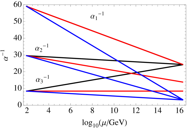
Figure 1: Evolution of the gauge coupling constants in the MSSM (black lines), the MSSM with the adjoint multiplets (red), and the MSSM with the adjoint and additional chiral multiplets (blue).

In this model, the strong interaction is not asymptotically free irrelevantly to the choice of the additional fields to recover the gauge coupling unification. Thus, the QCD corrections are large, and the masses of the colored particles tend to be large at the TeV scale, as compared to those in the MSSM. It is interesting to examine the extraordinary pattern of the mass spectrum of the colored particles for the hadron colliders. We, however, focus on the colorless fields; the $SU(2)_{L}$ triplet and singlet Higgs multiplets. These additional fields couple to the two MSSM Higgs doublets. Their coupling constants push up the SM-like Higgs boson mass due to the tree level $F$-term contribution, and thus the correct value of the Higgs boson mass (around $125~{}{\rm GeV}$) can be easily realized.

Furthermore, they cause mixing between the MSSM doublet Higgs fields and the additional Higgs fields, which results in modification of the coupling constants of the SM-like Higgs field. When such corrections are large enough to be detected at collider experiments, we can discriminate our model from other models by precisely measuring the pattern of the deviations in the Higgs coupling constants. In the next section, we will discuss these issues in more details.

One of the characteristic features of this model is that the coupling constants of the triplet and singlet Higgs multiplets are unified with the SM gauge coupling constants at the GUT scale. Thus, the low-energy values of these coupling constants in the Higgs sector are unambiguously determined by the RG running once the extra matters are specified.

For instance, taking the above example of the additional chiral matter multiplets to recover the gauge coupling unification, the Higgs sector coupling constants $\lambda_{\Delta}$ (red line) and $\lambda_{S}$ (blue), and the gauge coupling constants $g_{3,2,1}$ (green) evolve as shown in Fig. 2. Here, we normalize the singlet coupling as $\lambda^{\prime}_{S}=(2\sqrt{5/3})\lambda_{S}$, and the $U(1)_{Y}$ gauge coupling as $g_{1}=(\sqrt{5/3})g^{\prime}$, respectively, and one loop RGEs are used. For the list of the RGEs, see Appendix A. Since the $SU(2)_{L}$ gauge coupling is strong around the GUT scale, $\lambda_{\Delta}$ grows as the energy decreases. After the $SU(2)_{L}$ gauge coupling becomes weak, $\lambda_{\Delta}$ decreases as the energy decreases due to large trilinear couplings in the superpotential.

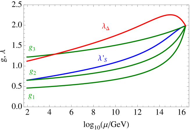
Figure 2: An example of running of the Higgs triplet and singlet coupling constants $\lambda_{\Delta}$ (red line) and $\lambda^{\prime}_{S}$ (blue) as well as the gauge coupling constants $g_{3}$, $g_{2}$ and $g_{1}$ (green) from the top to the bottom. The horizontal axis is the common logarithm of the energy scale in units of GeV. Here, we normalize the singlet and $U(1)_{Y}$ gauge couplings as $\lambda^{\prime}_{S}=(2\sqrt{5/3})\lambda_{S}$ and $g_{1}=(\sqrt{5/3})g^{\prime}$, respectively, and one loop RGEs are used.

We note that the triplet coupling $\lambda_{\Delta}$ remains in a perturbative region down to the TeV scale. At the TeV scale, we obtain

$$\lambda_{\Delta}=1.1\,,\qquad\lambda_{S}=0.25\,.$$ (9)

Similarly, the $\mu$-parameters of the adjoint chiral multiplets are unified at the GUT scale, and their ratio at the TeV scale is determined as $\mu_{S}:\mu_{\Delta}:\mu_{O}=1:2.9:230$, where $\mu_{O}$ stands for the octet $\mu$-parameter. The mass scale of the octet is far beyond the reach of collider experiments, as discussed qualitatively above.

Let us turn to the running of the soft SUSY breaking parameters. Since the unified gauge coupling is strong, the gaugino masses around the GUT scale must be large in order to avoid the experimental gluino mass limit LHCgluino . For instance, for the unified gaugino mass of $M_{1/2}=3600$ GeV, the gluino mass is pushed down to $m_{\tilde{g}}=1400$ GeV. As a result, soft mass parameters at the TeV scale are typically as large as $4$-$7$ TeV for colored particles and $1$-$2$ TeV for colorless particles. As in the MSSM, the soft mass squared of the up-type Higgs boson has a large contribution due to the large top Yukawa interaction. Therefore, some tuning is needed to realize electroweak symmetry breaking. The higgsino mass parameter $\mu$ and the CP-odd Higgs boson mass $m_{A}$ also tend to be $1$-$4$ TeV. In order to realize scenarios where some of the extra Higgs boson masses are of the order of ${\cal O}(100)$ GeV, further tuning is required among the input parameters.

III.2 Benchmark Points and the Mass of the SM-like Higgs boson

After the electroweak symmetry breaking, we obtain four CP-even, three CP-odd and three charged Higgs bosons as physical states in the Higgs sector, as well as six neutralinos and three charginos. Features of our model include new additional particles to the MSSM, and differences in the properties of the MSSM Higgs bosons. Among them, we here focus on the mass of the SM-like Higgs boson, which is determined by low energy soft SUSY breaking parameters obtained by solving the RGEs discussed above.

Before we discuss the cases where effects of the RG running is involved in calculating the SM-like Higgs boson mass, we exemplify rough predictions of our low energy effective theory without solving the RG equations. For relatively large triplet and singlet scalar masses, the SM-like Higgs boson mass is approximately written as Espinosa

$$m_{h}^{2}\simeq m_{Z}^{2}\cos^{2}\beta+\frac{3m_{t}^{4}}{2\pi^{2}v^{2}}\left(\ln{\frac{m_{\tilde{t}}^{2}}{m_{t}^{2}}}+\frac{X_{t}^{2}}{m_{\tilde{t}}^{2}}\left(1-\frac{X_{t}^{2}}{12m_{\tilde{t}}^{2}}\right)\right)+\frac{1}{8}\lambda_{\Delta}^{2}v^{2}\sin^{2}{2\beta}+\frac{1}{2}\lambda_{S}^{2}v^{2}\sin^{2}{2\beta}\,,$$ (10)

where $m_{Z}$ is the $Z$-boson mass, $m_{t}$ is the top quark mass, $m_{\tilde{t}}$ is the average of the two stop masses, and $X_{t}=A_{t}-\mu\cot\beta$ parametrizes mixing between the two stops. The first two terms correspond to the MSSM prediction. The last two terms originate from the existence of the trilinear couplings between the MSSM Higgs doublets and the additional triplet and singlet.

Within the MSSM, at the tree level the SM-like Higgs boson mass is smaller than the $Z$-boson mass. In order to reach $125~{}\rm{GeV}$ using the effect of the stop loop correction, the mass scale of the stops or the mixing parameter $X_{t}$ should be very large. For $X_{t}=0$, the stop mass should be of the order of $O(10)~{}\rm{TeV}$. Even in the maximum mixing case where $X_{t}=\pm\sqrt{6}m_{\tilde{t}}$, the stop mass is required to be as large as $O(1)~{}\rm{TeV}$MSSMHiggsMass2 . We also note that preferable range for $\tan\beta$ is larger than 10.

In our model, on the contrary, the predicted Higgs boson mass tends to be larger than that in the MSSM thanks to the tree level $F$-term contributions, in particular, for small $\tan\beta$ region. Such a result is reminiscent of the next-to-MSSM (NMSSMNMSSM ), where the SM-like Higgs boson mass is lifted up by coupling with a singlet superfield.

For computation of the masses of the Higgs scalars and superparticle, we have used the public numerical code SuSpect suspect , which takes the $\overline{\rm DR}$ renormalization scheme, instead of the approximate formula Eq.(10). We have appropriately modified SuSpect to add the new contributions from the Higgs trilinear couplings. Here, for simplicity, we have taken the limit $v_{\Delta}\to 0$. The computation of the SM-like Higgs boson mass including these triplet and singlet contributions is described in Appendix B. The LHC result $m_{h}=125~{}{\rm GeV}$ can be achieved even for small $\tan\beta$ and small stop mixing. We note that the formula given in Eq.(10) is valid when the neutral components of the triplet and singlet are heavier than the MSSM-like CP-even Higgs bosons. In general, the CP-even Higgs bosons mix with each other and the formulae for their mass eigenvalues are rather complicated.

Next, let us consider the mass of the SM-like Higgs boson including the radiative effects. As we mentioned, in order to have a successful electroweak symmetry breaking, fine tuning for input parameters at the GUT scale is required. Therefore, we will show some benchmark points that reproduce the mass of the SM-like Higgs boson, instead of scanning the parameter space. We focus on the following three different cases:

• All the Higgs bosons other than the SM-like Higgs boson are heavy.

• The new Higgs bosons other than the MSSM-like Higgs bosons are heavy.

• The new Higgs bosons affect the SM-like Higgs boson couplings.

Bearing the fact that there are a few GeV uncertainties in the numerical computation of the SM-like Higgs boson mass, we take the range of $122~{}{\rm GeV}<m_{h}<129~{}{\rm GeV}$ as its allowed region. Examples of successful benchmark points of input parameters at the GUT scale are listed in Tab. 2. Here, $\mu$ and $B$ parameters for the extra matters have insignificant effects on Higgs sector parameters, and are omitted from the list. Values of parameters of the TeV-scale effective theory are obtained after RG running and shown in Tab. 3. Definitions of the parameters are provided in Appendix A.

Case	$\tan\beta$	$M_{1/2}$	$\mu_{\Sigma}$
(A)(B)(C)	$3$	$3600~{}{\rm GeV}$	$-300~{}{\rm GeV}$

Case	$A_{0}$	$\widetilde{m}_{0}^{2}$	$\widetilde{m}_{H_{u}}^{2}$	$\widetilde{m}_{H_{d}}^{2}$	$\widetilde{m}_{5}^{2}$	$\widetilde{m}_{10}^{2}$	$\widetilde{m}_{\Sigma}^{2}$
(A)	$5500~{}{\rm GeV}$	$(1000~{}{\rm GeV})^{2}$	$(10375~{}{\rm GeV})^{2}$	$(8570~{}{\rm GeV})^{2}$	$-(6300~{}{\rm GeV})^{2}$	$-(2000~{}{\rm GeV})^{2}$	$-(570~{}{\rm GeV})^{2}$
(B)	$1000~{}{\rm GeV}$	$(1800~{}{\rm GeV})^{2}$	$(12604~{}{\rm GeV})^{2}$	$(10381.5~{}{\rm GeV})^{2}$	$-(7700~{}{\rm GeV})^{2}$	$-(1960~{}{\rm GeV})^{2}$	$-(670~{}{\rm GeV})^{2}$
(C)	$8000~{}{\rm GeV}$	$(3000~{}{\rm GeV})^{2}$	$(10605.1~{}{\rm GeV})^{2}$	$(8751.4~{}{\rm GeV})^{2}$	$-(6418~{}{\rm GeV})^{2}$	$-(1638.5~{}{\rm GeV})^{2}$	$-(400~{}{\rm GeV})^{2}$

Table 2: Benchmark points of input parameters at the GUT scale.

Case	$M_{1}$	$M_{2}$	$M_{3}$	$\mu_{\Delta}$	$\mu_{S}$
(A)(B)(C)	$194~{}{\rm GeV}$	$388~{}{\rm GeV}$	$1360~{}{\rm GeV}$	$-252~{}{\rm GeV}$	$-85.8~{}{\rm GeV}$

Case	$\mu$	$B\mu$	$\widetilde{m}_{u_{3}}$	$\widetilde{m}_{q_{3}}$	$y_{t}A_{t}$
(A)	$205~{}{\rm GeV}$	$41400~{}{\rm GeV}^{2}$	$3290~{}{\rm GeV}$	$4830~{}{\rm GeV}$	$4030~{}{\rm GeV}$
(B)	$177~{}{\rm GeV}$	$40800~{}{\rm GeV}^{2}$	$1730~{}{\rm GeV}$	$4480~{}{\rm GeV}$	$6050~{}{\rm GeV}$
(C)	$174~{}{\rm GeV}$	$42000~{}{\rm GeV}^{2}$	$4220~{}{\rm GeV}$	$5550~{}{\rm GeV}$	$2910~{}{\rm GeV}$

Case	$\widetilde{m}_{\Delta}$	$\widetilde{m}_{S}$	$\lambda_{\Delta}A_{\Delta}$	$\lambda^{\prime}_{S}A_{S}$	$B_{\Delta}\mu_{\Delta}$	$B_{S}\mu_{S}$	$m_{h}$
(A)	$607~{}{\rm GeV}$	$805~{}{\rm GeV}$	$662~{}{\rm GeV}$	$683~{}{\rm GeV}$	$92000~{}{\rm GeV}^{2}$	$-78700~{}{\rm GeV}^{2}$	$123~{}{\rm GeV}$
(B)	$784~{}{\rm GeV}$	$612~{}{\rm GeV}$	$1340~{}{\rm GeV}$	$1110~{}{\rm GeV}$	$30700~{}{\rm GeV}^{2}$	$-110000~{}{\rm GeV}^{2}$	$123~{}{\rm GeV}$
(C)	$521~{}{\rm GeV}$	$216~{}{\rm GeV}$	$284~{}{\rm GeV}$	$446~{}{\rm GeV}$	$207000~{}{\rm GeV}^{2}$	$-33600~{}{\rm GeV}^{2}$	$122~{}{\rm GeV}$

Table 3: Parameters of the TeV-scale effective theory obtained after RG running.

IV Impact on Higgs Properties

In this section, we discuss properties of the particles in the Higgs sector. We will show that our model can be distinguished from other new physics models by measuring the masses and the coupling constants of the Higgs sector particles at the LHC and future electron-positron colliders HiggsWG ; ILC ; CLIC ; ILCHiggs . Even in the cases where the additional Higgs particles are beyond the reach of direct discovery at these colliders, the existence of these new particles can be indirectly probed by precise measurements of the coupling constants of the discovered SM-like Higgs boson and MSSM Higgs boson masses.

IV.1 Vertices of the SM-like Higgs boson

First, we address the couplings between the SM-like Higgs boson and SM particles, which have been already measured to some extent at the LHC. So far, no deviation that obviously contradicts the SM predictions has been reported. In the future, precision of these observables will be significantly improved by the high-luminosity LHC and the ILC, and therefore this method serves as a powerful tool in discriminating beyond-the-SM models.

Discarding the VEV of the triplet Higgs boson, the Higgs boson coupling with the $W$- or $Z$-boson is given by

$$g_{hVV}=g_{V}m_{V}(R_{11}^{S}\cos\beta+R_{12}^{S}\sin\beta)\,,\quad V=W,Z$$ (11)

those with the up-type quarks, down-type quarks and charged leptons by

$$g_{huu}=\frac{\sqrt{2}m_{u}}{v}\frac{R_{12}^{S}}{\sin\beta}\,,\quad g_{hdd}=\frac{\sqrt{2}m_{d}}{v}\frac{R_{11}^{S}}{\cos\beta}\,,\quad g_{h\ell\ell}=\frac{\sqrt{2}m_{\ell}}{v}\frac{R_{11}^{S}}{\cos\beta}\,,$$ (12)

respectively, and the Higgs self-coupling is

$$g_{hhh}=\sum_{a,b,c}R_{1a}^{S}R_{1b}^{S}R_{1c}^{S}\lambda_{s_{a}s_{b}s_{c}}\,,$$ (13)

where $R^{S}$ denotes the orthogonal matrix that diagonalizes the CP-even Higgs mass matrix, and $\lambda_{s_{a}s_{b}s_{c}}$ are tree-level couplings among CP-even Higgs bosons in the gauge basis. Their definitions are summarized in Appendix B. The effective vertex of $h\gamma\gamma$ including contributions from the additional charged Higgs bosons is given by

$$g_{h\gamma\gamma}=\sum_{f}N_{c}Q_{f}^{2}g_{hff}A_{1/2}(\tau_{f})+g_{hWW}A_{1}(\tau_{W})+\sum_{h^{\pm}_{i}}\frac{m_{W}^{2}\lambda_{hh^{+}_{i}h^{-}_{i}}}{2c_{W}^{2}m_{h^{\pm}_{i}}^{2}}A_{0}(\tau_{h^{\pm}_{i}})\,,$$ (14)

where the number of color is $N_{c}=3$, and $Q_{f}$ denote the electric charges of fermions $f$. For the definitions of the amplitudes $A_{i}$, see, for example, Ref. Djouadi:2005gj . The Higgs boson couplings with the charged Higgs bosons are given by

$$\lambda_{hh^{+}_{i}h^{-}_{i}}=\sum_{a,b,c}R_{1a}^{S}U_{ib}^{C*}U_{ic}^{C}\lambda_{s_{a}w^{+}_{b}w^{-}_{c}}\,.$$ (15)

The definitions of the unitary matrix $U^{C}$ and couplings $\lambda_{s_{a}w^{+}_{b}w^{-}_{c}}$ are summarized in Appendix B.

The corresponding couplings in the SM are

$${g_{hVV}|_{\rm SM}}=g_{V}m_{V},\quad{g_{huu}|_{\rm SM}}=\frac{\sqrt{2}m_{u}}{v}\,,\quad{g_{hdd}|_{\rm SM}}=\frac{\sqrt{2}m_{d}}{v}\,,$$

$${g_{h\ell\ell}|_{\rm SM}}=\frac{\sqrt{2}m_{\ell}}{v}\,,\quad{g_{hhh}|_{\rm SM}}=\frac{m_{Z}^{2}}{v}\,.$$ (16)

It is useful to define deviation parameters

$$\kappa_{X}=\frac{g_{hXX}}{g_{hXX}|_{\rm SM}}\,,$$ (17)

where $X$ denotes SM particles. Such deviations are extracted from measurements of the decay widths of the Higgs boson.

In Fig. 3, the deviations in the Higgs boson coupling with the tau lepton $\kappa_{\tau}$ and that with the bottom quark $\kappa_{b}$ from the SM predictions are plotted. The predictions of the three benchmark points (A), (B) and (C) in the SGGHU are shown with green blobs. The MSSM and NMSSM predictions are shown with red and blue lines, respectively. Here, we simply adjust the stop masses and mixing so that the observed Higgs boson mass is reproduced. In our model, the Higgs boson couplings to the down-type quarks and charged leptons are common and fall in the category of the two Higgs doublet model. Therefore, the predicted SGGHU deviations lie on the MSSM and NMSSM lines, as is evident from Eq.(12). The recent LHC results show strong evidence of the Higgs boson coupling with the tau lepton consistent with the SM prediction LHCtau . At the ILC with $\sqrt{s}=500~{}{\rm GeV}$, expected accuracies for the deviations $\kappa_{\tau}$ and $\kappa_{b}$ are 2.3% and 1.6%, respectively ILCHiggs .

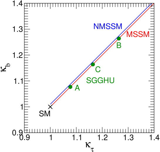
Figure 3: The deviations in the Higgs boson coupling with the tau lepton $\kappa_{\tau}$ and that with the bottom quark $\kappa_{b}$ from the SM predictions are plotted. The predictions of the three benchmark points (A), (B) and (C) in the SGGHU are shown with green blobs. The MSSM and NMSSM predictions are shown with red and blue lines, respectively. For the purpose of illustration, the NMSSM line is slightly displaced from $\kappa_{\tau}=\kappa_{b}$.

In Fig. 4, the deviations in the Higgs boson coupling with the weak gauge bosons $\kappa_{V}$ and that with the bottom quark $\kappa_{b}$ from the SM predictions are plotted. The predictions of the three benchmark points (A), (B) and (C) in the SGGHU are shown with green blobs. The MSSM predictions are shown with red lines for $\tan\beta=10$ (thick line) and $\tan\beta=3$ (dashed). The NMSSM predictions are shown with blue grid lines, which indicate mixings between the SM-like and singlet like Higgs bosons of 10%, 20% and 30% from the right to the left. As is reported in Ref.ILCHiggs , the ILC with $\sqrt{s}=500~{}{\rm GeV}$ can reach accuracy of 1.0% (1.1%) for the Higgs boson coupling with the $Z$-boson (the $W$-boson). Therefore, signatures different from the MSSM and its variants are expected to be observed using $\kappa_{V}$ at the ILC. Notice that the VEV of the triplet Higgs boson $v_{\Delta}$ is small compared to those of the doublet Higgs bosons. Therefore, the mixing between the SM-like Higgs boson and the CP-even component of the Higgs singlet dominates over that between the SM-like Higgs boson and the triplet component. In this sense, our model is similar to the NMSSM. It will be difficult to distinguish our model only from these observables.

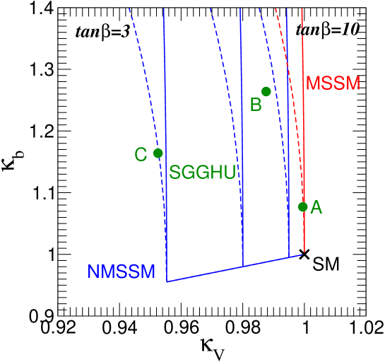
Figure 4: The deviations in the Higgs boson coupling with the weak gauge bosons $\kappa_{V}$ and that with the bottom quark $\kappa_{b}$ from the SM predictions are plotted. The predictions of the three benchmark points (A), (B) and (C) in the SGGHU are shown with green blobs. The MSSM predictions are shown with red lines for $\tan\beta=10$ (thick line) and $\tan\beta=3$ (dashed). The NMSSM predictions are shown with blue grid lines, which indicate mixings between the SM-like and singlet like Higgs bosons of 10%, 20% and 30% from the right to the left.

In Fig. 5, the deviations in the Higgs boson coupling with the charm quark $\kappa_{c}$ and that with the bottom quark $\kappa_{b}$ from the SM predictions are plotted. As in Fig. 4, the predictions of the three benchmark points (A), (B) and (C) in the SGGHU are shown with green blobs, and the MSSM and NMSSM predictions are shown with red and blue lines, respectively. In sharp contrast to the $\kappa_{V}$-$\kappa_{b}$ relation, correlations between $\kappa_{c}$ and $\kappa_{b}$ strongly depend on the value of $\tan\beta$. For example, the benchmark point (C) with $\tan\beta=3$ is not covered by the NMSSM predictions with $\tan\beta=10$, and the deviation can be measured at the ILC with $\sqrt{s}=500~{}{\rm GeV}$, which aims to measure $\kappa_{c}$ with accuracy of 2.8%. Independent $\tan\beta$ measurement using decay of the Higgs boson at the ILC Gunion:2002ip ; Kanemura:2013eja will also play an important role in discriminating models. Although it will be difficult to completely distinguish our model from the NMSSM from the precision measurements of Higgs boson couplings, if the deviation pattern of the Higgs couplings is found to be close to our benchmark points, there is a fair possibility that the SGGHU is realized. The ILC is absolutely necessary for investigating the Higgs properties and distinguishing particle physics models.

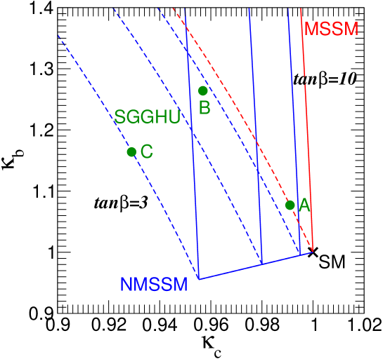
Figure 5: The deviations in the Higgs boson coupling with the charm quark $\kappa_{c}$ and that with the bottom quark $\kappa_{b}$ from the SM predictions are plotted. See the caption of Fig. 4 for details.

As for other Higgs boson couplings, the deviations of the Higgs boson coupling with the photon are $0.94<\kappa_{\gamma}<1.0$, and those of the Higgs self-coupling $0.82<\kappa_{h}<0.93$ for the benchmark points we show. To observe deviations in these observables from the SM predictions one needs more precise measurements at the ILC with $\sqrt{s}=1~{}{\rm TeV}$ ILCHiggs .

IV.2 Additional Higgs bosons

Finally, we mention the additional MSSM-like Higgs bosons. Since four-point couplings in the Higgs sector are expressed in terms of gauge couplings and $F$-term couplings in SUSY models, differences of the masses of the MSSM-like Higgs bosons are also useful measures in probing more fundamental physics. The MSSM-like charged Higgs boson mass $m_{H^{\pm}}$ is given by

$$m_{H^{\pm}}^{2} =m_{H^{\pm}}^{2}|_{\rm MSSM}(1+\delta_{H^{\pm}})^{2}$$

$$\simeq m_{A}^{2}+m_{W}^{2}+\frac{1}{8}\lambda_{\Delta}^{2}v^{2}-\frac{1}{2}\lambda_{S}^{2}v^{2}\,,$$ (18)

where $\delta_{H^{\pm}}$ is the deviation in $m_{H^{\pm}}$ from the MSSM and $m_{A}$ is the MSSM-like CP-odd Higgs boson mass. The sign of the singlet contribution is opposite to the triplet one due to the group theory. From Eq. (9), $m_{H^{\pm}}$ becomes large as compared to the MSSM. We emphasize that these $\lambda_{S}$ and $\lambda_{\Delta}$ couplings are determined by the RGEs and a larger $m_{H^{\pm}}$ is a prediction in this model. The charged Higgs boson is always heavier than the CP-odd Higgs boson. Since $m_{H^{\pm}}|_{\rm MSSM}$ is the sum of $m_{A}$ and $m_{W}$, when the CP-odd Higgs boson and the charged Higgs boson are discovered, we can obtain $\delta_{H^{\pm}}$ by measuring $m_{A}$ and $m_{H^{\pm}}$ precisely. Fig. 6 shows the deviation parameter $\delta_{H^{\pm}}$ of the MSSM-like charged Higgs boson mass $m_{H^{\pm}}$ as a function of $m_{A}$ in the large soft mass scenario. The black, blue and green lines correspond to triplet contribution, singlet contribution, sum of the singlet and triplet contributions, respectively. Here, we choose $\lambda_{\Delta}=1.1$ and $\lambda_{S}=0.25$. The mass deviation is found to be $O(1)~{}\%$ - $O(10)~{}\%$ if the mass scale of the MSSM-like Higgs bosons are below $500~{}{\rm GeV}$. On the other hand, the deviation in the heavy CP-even Higgs boson mass $m_{H}$ from the MSSM prediction is less than $O(1)~{}\%$. Since the charged Higgs boson mass can be determined with an accuracy of a few percent at the LHC given such small masses HiggsWG , we can test our model.

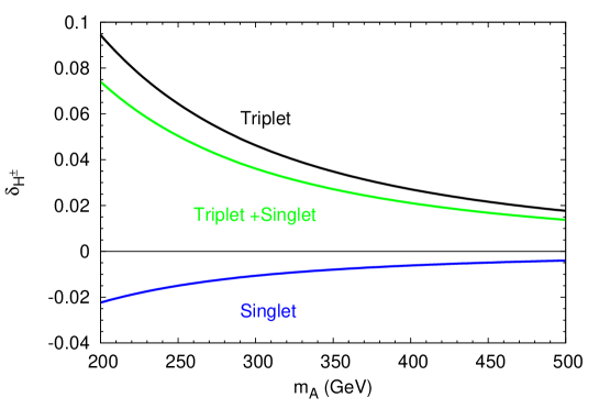
Figure 6: The deviation parameter $\delta_{H^{\pm}}$ of the MSSM-like charged Higgs boson mass $m_{H^{\pm}}$ as a function of the MSSM-like CP-odd Higgs boson mass $m_{A}$ in the large soft mass scenario. The black, blue and green lines correspond to triplet contribution, singlet contribution, sum of the singlet and triplet contributions, respectively. Here, we choose $\lambda_{\Delta}=1.1$ and $\lambda_{S}=0.25$.

When the masses of the triplet-like and singlet-like scalar bosons are below $500~{}{\rm GeV}$, the ILC and CLIC have capability to directly produce these new particles. For example, the benchmark point (C) gives mass spectrum of the Higgs sector particles shown in Tab. 4. In this case, the mass of the lighter triplet-like Higgs boson $\Delta^{\pm}$ is less than $500~{}{\rm GeV}$, and we can probe $\Delta^{\pm}$ using the channel $e^{+}e^{-}\rightarrow\Delta^{+}\Delta^{-}\rightarrow tb\bar{t}\bar{b}$, which proceeds via the mixing between the MSSM-like and triplet-like charged Higgs bosons.

CP-even	CP-odd	Charged
$122~{}{\rm GeV}$	$-$	$-$
$139~{}{\rm GeV}$	$171~{}{\rm GeV}$	$204~{}{\rm GeV}$
$370~{}{\rm GeV}$	$304~{}{\rm GeV}$	$496~{}{\rm GeV}$
$745~{}{\rm GeV}$	$497~{}{\rm GeV}$	$745~{}{\rm GeV}$

Table 4: Mass spectrum of the Higgs scalars for the benchmark point (C).

V Discussion and Conclusion

In this paper, we have investigated phenomenology of the Higgs sector of the supersymmetric version of the grand gauge-Higgs unification model, where the $SU(5)$ grand unified gauge symmetry is broken by the Hosotani mechanism. Our model provides a natural solution to the doublet-triplet splitting problem thanks to the phase nature of the Hosotani mechanism, and predicts existence of a light color octet, an $SU(2)_{L}$ triplet and a neutral singlet chiral multiplets whose masses are around the TeV scale. Since the adjoint chiral multiplets are originated from the GUT gauge multiplet, there are no trilinear self-couplings among them and their couplings to MSSM fields are unified to the SM gauge coupling constants at the GUT scale. Therefore, our model is highly predictive. We have performed RGE analysis to obtain masses and coupling constants of the low-energy effective theory of our model. Although the mass scale of the color octet chiral multiplet is found to be beyond reach of collider experiments, the masses of the triplet and singlet multiplets can remain as small as those of the MSSM Higgs doublets, and thus the Higgs sector is extended by these new Higgs multiplets.

We have computed the SM-like Higgs boson mass including tree level and one loop level contributions from the triplet and singlet couplings, and shown benchmark points consistent with the LHC Higgs boson mass measurements. Based on the benchmark points, we have evaluated deviations of couplings between the Higgs boson and SM particles from the corresponding SM values, which are one of the main targets of the future ILC project. The deviations of the couplings from the SM predictions turn out to be ${\cal O}(1)\%$ when the triplet and singlet Higgs boson masses are below $\simeq 1~{}{\rm TeV}$. Given such small masses, we can distinguish our model, MSSM and NMSSM by comparing patterns of the deviations of these new physics models. As for additional Higgs bosons, the mass gap between the MSSM-like charged Higgs boson and the MSSM-like CP-odd Higgs boson differs from that of the MSSM by ${\cal O}(1)\%$ - ${\cal O}(10)\%$ when their masses are below $\simeq 500~{}{\rm GeV}$. Such a deviation is within the scope of the LHC.

Last but not least, the extension of the Higgs sector in SUSY models means that the neutralino and chargino sectors are also extended. For the benchmark points we have shown, masses of the six neutralinos and three charginos are all less than $500~{}{\rm GeV}$. Collider signatures of such additional neutralinos and charginos will be discussed elsewhere.

We emphasize that our supersymmetric grand gauge-Higgs unification model serves as a good example of grand unification that is testable at future electron-positron colliders, and researches along this strategy should be encouraged.

Appendix A Renormalization Group Equations

In this appendix, we summarize the one loop RGEs between the SUSY scale and the GUT scale for our model. Here, for later reference, we give them in a form which correctly includes the flavor structure though it is less relevant to our analysis in this article.

A.1 Notations

In order to treat the flavor, it is convenient to use a notation different from the one used in the main text for the $A$- and $B$-terms so that the corresponding SUSY parameters are not extracted. To distinguish them, we append a bar on top of the $A$- and $B$-terms used in this appendix. Namely, for example the $B$-term of the singlet is defined as $\bar{B}_{S}=B_{S}\mu_{S}$.

The flavor structure is expressed by using 3-by-3 matrices as usual. Here we use the character $Y$ for the Yukawa couplings with the flavor and thus $Y$ is treated as a matrix, and the character $\lambda$ for those without the flavor. The character $y$ denotes all the Yukawa coupling, $Y$ and $\lambda$, symbolically. A dot on a parameter $P(Q)$ is used for a partial derivative by the renormalization scale $Q$ with a normalization factor: $(16\pi^{2})\partial P/\partial\ln(Q/Q_{0})$ where $Q_{0}$ is an arbitrary reference scale.

The superpotential we consider is

$$W=W^{\rm matter}+W^{\rm Higgs}+W^{add},$$ (19)

with

$$W^{\rm matter}=uY_{u}q\cdot H_{u}-dY_{d}q\cdot H_{d}-eY_{e}\ell\cdot H_{d},$$ (20)

$W^{\rm Higgs}$ is given in Eq. (4) and

$$W^{add}=\bar{L}_{j}\cdot(\lambda_{L_{j}\Delta}\Delta-\lambda_{L_{j}S}S+\mu_{L_{j}})L_{j}+\bar{U}(\lambda_{UG}G-\frac{4}{3}\lambda_{US}S+\mu_{U})U$$

$$+(2\lambda_{ES}S+\mu_{E})\bar{E}E+\mu_{G}{\rm{tr}}(GG).$$ (21)

Here, $q$, $u$, $d$, $\ell$ and $e$ denote the MSSM matter chiral multiplets, $Y_{x}$ ($x=u,d,e$) is a $3\times 3$ matrix, $S$, $\Delta$ and $G$ are the adjoint chiral multiplets and $(\bar{L}_{j},\ L_{j})$ ($j=1,2$), $(\bar{U},\ U)$ and $(\bar{E},\ E)$ are the additional vectorlike pairs introduced to recover the gauge coupling unification.

The SUSY-breaking soft terms contain the tadpole term of $S$, aside from the usual soft mass squared terms, $A$-terms and $B$-terms:

$$V_{\rm soft}=V^{\rm matter}_{\rm soft}+V^{\rm Higgs}_{\rm soft}+V^{add}_{\rm soft},$$ (22)

with

$$V^{\rm matter}_{\rm soft}=\tilde{q}^{\dagger}\tilde{m}^{2}_{q}\tilde{q}+\tilde{u}^{T}\tilde{m}^{2}_{u}\tilde{u}^{*}+\tilde{d}^{T}\tilde{m}^{2}_{d}\tilde{d}^{*}+\tilde{\ell}^{\dagger}\tilde{m}^{2}_{\ell}\tilde{\ell}+\tilde{e}^{T}\tilde{m}^{2}_{e}\tilde{e}^{*}$$

$$+\left[u\bar{A}_{u}q\cdot H_{u}-d\bar{A}_{d}q\cdot H_{d}-e\bar{A}_{e}\ell\cdot H_{d}+{\rm h.c.}\right],$$ (23)

$V^{\rm Higgs}_{\rm soft}$ is given in Eq. (5) and

$$V^{add}_{\rm soft}=\tilde{m}^{2}_{L_{j}}\left|L_{j}\right|^{2}+\tilde{m}^{2}_{\bar{L}_{j}}\left|\bar{L}_{j}\right|^{2}+\tilde{m}^{2}_{U}\left|U\right|^{2}+\tilde{m}^{2}_{\bar{U}}\left|\bar{U}\right|^{2}+\tilde{m}^{2}_{E}\left|E\right|^{2}+\tilde{m}^{2}_{\bar{E}}\left|\bar{E}\right|^{2}+\tilde{m}^{2}_{G}\left|G\right|^{2}$$

$$+\left[\bar{L}_{j}\cdot(\bar{A}_{L_{j}\Delta}\Delta-\bar{A}_{L_{j}S}S+\bar{B}_{L_{j}})L_{j}+\bar{U}(\bar{A}_{UG}G-\frac{4}{3}\bar{A}_{US}S+\bar{B}_{U})U\right.$$

$$\left.+(2\bar{A}_{ES}S+\bar{B}_{E})\bar{E}E+\bar{B}_{G}{\rm{tr}}(GG)+{\rm h.c.}\right].$$ (24)

It is worthwhile to notice that the tadpole term of the scalar component of $S$ in $V_{\rm soft}^{Higgs}$ is generated even the tadpole term in the superpotential is forbidden, while that of the $F$-component of $S$ can be removed by a field redefinition. Since the latter is generated by the loop corrections, we have to do the field redefinition at each scale, and the RGEs of the $B$-terms for the fields that couple to $S$ are affected.

A.2 RGEs

The formalism including some notations in this subsection is the one in Ref. BY

A.2.1 Gauge Couplings and Gaugino Masses

The RGEs for the gauge couplings $g_{i}$ and the gaugino masses $M_{i}$ are given as

$$\dot{g}_{i}\, = \,b_{i}\,g_{i}^{3},$$

$$\dot{M}_{i} = 2b_{i}\,g_{i}^{2}M_{i},$$ (25)

with the beta function coefficients $b_{i}$. In this model they are $b_{i}=(\frac{53}{5},5,1)$.

A.2.2 Yukawa Couplings

The RGEs for the Yukawa couplings:

$$\dot{Y}_{u} =\gamma^{T}_{u}Y_{u}+Y_{u}\gamma_{q}+\gamma_{H_{u}}Y_{u},$$ (26)

$$\dot{Y}_{d} =\gamma^{T}_{d}Y_{d}+Y_{d}\gamma_{q}+\gamma_{H_{d}}Y_{d},$$

$$\dot{Y}_{e} =\gamma^{T}_{e}Y_{e}+Y_{e}\gamma_{\ell}+\gamma_{H_{d}}Y_{e},$$

$$\dot{\lambda}_{\Delta} =(\gamma_{H_{u}}+\gamma_{H_{d}}+\gamma_{\Delta})\lambda_{\Delta},$$

$$\dot{\lambda}_{S} =(\gamma_{H_{u}}+\gamma_{H_{d}}+\gamma_{S})\lambda_{S},$$

$$\dot{\lambda}_{L_{j}\Delta} =(\gamma_{L_{j}}+\gamma_{\bar{L}_{j}}+\gamma_{\Delta})\lambda_{L_{j}\Delta},$$

$$\dot{\lambda}_{L_{j}S} =(\gamma_{L_{j}}+\gamma_{\bar{L}_{j}}+\gamma_{S})\lambda_{L_{j}S},$$

$$\dot{\lambda}_{UG} =(\gamma_{U}+\gamma_{\bar{U}}+\gamma_{G})\lambda_{UG},$$

$$\dot{\lambda}_{US} =(\gamma_{U}+\gamma_{\bar{U}}+\gamma_{S})\lambda_{US},$$

$$\dot{\lambda}_{ES} =(\gamma_{E}+\gamma_{\bar{E}}+\gamma_{S})\lambda_{ES},$$

with the anomalous dimensions $\gamma$, among which $\gamma_{f}$ ($f=q,u,d,\ell,e$) is a $3\times 3$ matrix.

$$\gamma_{q} =-2\left(\displaystyle{\frac{4}{3}}g^{2}_{3}+\frac{3}{4}g^{2}_{2}+\frac{1}{60}g^{2}_{1}\right)\!{\mathop{\bf 1}}+Y_{u}^{\dagger}Y_{u}+Y_{d}^{\dagger}Y_{d},$$ (27)

$$\gamma_{u} =-2\left(\displaystyle{\frac{4}{3}}g^{2}_{3}+\frac{4}{15}g^{2}_{1}\right)\!{\mathop{\bf 1}}+2Y_{u}^{\ast}Y_{u}^{T},$$

$$\gamma_{d} =-2\left(\displaystyle{\frac{4}{3}}g^{2}_{3}+\frac{1}{15}g^{2}_{1}\right)\!{\mathop{\bf 1}}+2Y_{d}^{\ast}Y_{d}^{T},$$

$$\gamma_{\ell} =-2\left(\displaystyle{\frac{3}{4}}g^{2}_{2}+\frac{3}{20}g^{2}_{1}\right)\!{\mathop{\bf 1}}+Y_{e}^{\dagger}Y_{e},$$

$$\gamma_{e} =-2\left(\displaystyle{\frac{3}{5}}g^{2}_{1}\right)\!{\mathop{\bf 1}}+2Y_{e}^{\ast}Y_{e}^{T},$$

$$\gamma_{H_{u}} =-2\left(\displaystyle{\frac{3}{4}}g^{2}_{2}+\frac{3}{20}g^{2}_{1}\right)+{\rm Tr}\left(3Y_{u}^{\dagger}Y_{u}\right)+\delta\gamma_{H},$$

$$\gamma_{H_{d}} =-2\left(\displaystyle{\frac{3}{4}}g^{2}_{2}+\frac{3}{20}g^{2}_{1}\right)+{\rm Tr}\left(3Y_{d}^{\dagger}Y_{d}+Y_{e}^{\dagger}Y_{e}\right)+\delta\gamma_{H},$$

$$\delta\gamma_{H} =\left|\lambda_{S}\right|^{2}+\frac{3}{4}\left|\lambda_{\Delta}\right|^{2},$$ (28)

$$\gamma_{S} =2\left|\lambda_{S}\right|^{2}+\sum_{j}2\left|\lambda_{L_{j}S}\right|^{2}+\frac{16}{3}\left|\lambda_{US}\right|^{2}+4\left|\lambda_{ES}\right|^{2},$$

$$\gamma_{\Delta} =-2\left(\displaystyle{2}g^{2}_{2}\right)+\frac{1}{2}\left|\lambda_{\Delta}\right|^{2}+\sum_{j}\frac{1}{2}\left|\lambda_{L_{j}\Delta}\right|^{2},$$

$$\gamma_{G} =-2\left(\displaystyle{3}g^{2}_{3}\right)+\frac{1}{2}\left|\lambda_{UG}\right|^{2},$$

$$\gamma_{L_{j}}=\gamma_{\bar{L}_{j}} =-2\left(\displaystyle{\frac{3}{4}}g^{2}_{2}+\frac{3}{20}g^{2}_{1}\right)+\left|\lambda_{L_{j}S}\right|^{2}+\frac{3}{4}\left|\lambda_{L_{j}\Delta}\right|^{2},$$

$$\gamma_{U}=\gamma_{\bar{U}} =-2\left(\displaystyle{\frac{4}{3}}g^{2}_{3}+\frac{4}{15}g^{2}_{1}\right)+\frac{16}{9}\left|\lambda_{US}\right|^{2}+\frac{4}{3}\left|\lambda_{UG}\right|^{2},$$

$$\gamma_{E}=\gamma_{\bar{E}} =-2\left(\frac{3}{5}g^{2}_{1}\right)+4\left|\lambda_{ES}\right|^{2}.$$

A.2.3 $\mu$-terms

Similarly, the supersymmetric mass terms evolve as

$$\dot{\mu} =\left(\gamma_{H_{u}}+\gamma_{H_{d}}\right)\mu,$$ (29)

$$\dot{\mu_{S}} =2\gamma_{S}\mu_{S},$$

$$\dot{\mu_{\Delta}} =2\gamma_{\Delta}\mu_{\Delta},$$

$$\dot{\mu_{G}} =2\gamma_{G}\mu_{G},$$

$$\dot{\mu_{L_{j}}} =\left(\gamma_{\bar{L}_{j}}+\gamma_{L_{j}}\right)\mu_{L_{j}},$$

$$\dot{\mu_{U}} =\left(\gamma_{\bar{U}}+\gamma_{U}\right)\mu_{U},$$

$$\dot{\mu_{E}} =\left(\gamma_{\bar{E}}+\gamma_{E}\right)\mu_{E}.$$

A.2.4 $A$-terms

The RGEs for the $A$-terms can be derived from those for the corresponding Yukawa couplings given in Eq. (26) which are functions of the Yukawa couplings $y$ and the anomalous dimensions $\gamma$, $\dot{y}(y,\gamma)$, by

$$\dot{\bar{A}}_{x}=\dot{y}_{x}|_{y\to\bar{A}}+\dot{y}_{x}|_{\gamma\to\tilde{\gamma}}=\dot{y}_{x}(\bar{A},\gamma)+\dot{y}_{x}(y,\tilde{\gamma}).$$ (30)

Here, the quantities $\tilde{\gamma}_{f}$ can be built from the corresponding anomalous dimensions in Eqs. (27) and (28) with the replacements:

$$g_{i}^{2}\to-2g_{i}^{2}M_{i},\hskip 28.45274pty_{x}^{\dagger}y_{x}\to 2y_{x}^{\dagger}\bar{A}_{x},\hskip 28.45274pty_{x}^{\ast}y_{x}^{T}\to 2y_{x}^{\ast}\bar{A}_{x}^{T}.$$ (31)

A.2.5 $B$-terms

Similarly, the RGEs for the $B$-terms are obtained from those for the corresponding $\mu$-terms in Eq. (29), but with further contribution due to the field redefinition of $S$ as

$$\dot{\bar{B}}_{f}=\dot{\mu}_{f}|_{\mu\to\bar{B}}+\dot{\mu}_{f}|_{\gamma\to\tilde{\gamma}}+\lambda_{fS}J_{S}.$$ (32)

Here, $\lambda_{fS}$ is the Yukawa couplings among the relevant vectorlike pair and the singlet $S$, and the quantity $J_{S}$ is built from $\gamma_{S}$ in Eq. (28) with the replacement

$$\left|\lambda_{fS}\right|^{2}\to 2\lambda_{fS}^{*}\bar{B}_{f}.$$ (33)

A.2.6 Scalar Tadpole

The RGE for the scalar tadpole of $S$ is written by

$$\dot{\xi}=\gamma_{S}\xi+\tilde{J}_{S}^{*}+J_{S}\mu_{S},$$ (34)

with $\tilde{J}_{S}$ built from $\gamma_{S}$ in Eq. (28) with the replacement

$$\left|\lambda_{fS}\right|^{2}\to 2\left(\lambda_{fS}^{\dagger}\left(\tilde{m}^{2}_{f}+\tilde{m}^{2}_{\bar{f}}\right)\mu_{f}+\bar{A}_{fS}^{*}\bar{B}_{f}\right),$$ (35)

where $\tilde{m}^{2}_{f}$ and $\tilde{m}^{2}_{\bar{f}}$ are the masses squared of the relevant vectorlike pair.

A.3 Scalar Soft Squared Masses

It is convenient to define a function ${\cal F}$:

$${\cal F}(y_{x}^{\dagger},f_{1},f_{2},f_{3},\bar{A}_{x}^{\dagger}) = y_{x}^{\dagger}y_{x}\widetilde{m}^{2}_{f_{1}}+\widetilde{m}^{2}_{f_{1}}y_{x}^{\dagger}y_{x}$$ (36)

$$+2\left(y_{x}^{\dagger}\widetilde{m}^{2\,\ast}_{f_{2}}y_{x}+\!\widetilde{m}^{2}_{f_{3}}y_{x}^{\dagger}y_{x}+\!\bar{A}_{x}^{\dagger}\bar{A}_{x}\right),\quad$$

where $y_{x}$ is any of the Yukawa couplings in the superpotential, $\tilde{m}^{2}_{f_{1}}$ is the mass squared for which the RGE in question is derived, $\tilde{m}^{2}_{f_{2}}$ and $\tilde{m}^{2}_{f_{3}}$ are the masses squared of the particles exchanged in the loops that induce the RGE. Since the order of $f_{1},f_{2},f_{3}$ is not important when $y_{x}$ is some of $\lambda$, the order may be changed below.

Using the function $\cal F$, the RGEs for the soft squared masses are written as

$$\dot{\widetilde{m}}^{2}_{q}\, =-8\left(\frac{4}{3}g^{2}_{3}M_{3}^{2}+\frac{3}{4}g^{2}_{2}M_{2}^{2}+\frac{1}{60}g^{2}_{1}M_{1}^{2}\right)\!{\mathop{\bf 1}}+{\cal F}(Y_{u}^{\dagger},{q},{u},H_{u},\bar{A}_{u}^{\dagger})+{\cal F}(Y_{d}^{\dagger},{q},{d},H_{d},\bar{A}_{d}^{\dagger}),$$ (37)

$$\dot{\widetilde{m}}_{u}^{2} =-8\left(\frac{4}{3}g^{2}_{3}M_{3}^{2}+\frac{4}{15}g^{2}_{1}M_{1}^{2}\right)\!{\mathop{\bf 1}}+2{\cal F}{(Y_{u},{u},{q},H_{u},\bar{A}_{u})},$$

$$\dot{\widetilde{m}}_{d}^{2} =-8\left(\frac{4}{3}g^{2}_{3}M_{3}^{2}+\frac{1}{15}g^{2}_{1}M_{1}^{2}\right)\!{\mathop{\bf 1}}+2{\cal F}{(Y_{d},{d},{q},H_{d},\bar{A}_{d})},$$

$$\dot{\widetilde{m}}_{\ell}^{2} =-8\left(\frac{3}{4}g^{2}_{2}M_{2}^{2}+\frac{3}{20}g^{2}_{1}M_{1}^{2}\right)\!{\mathop{\bf 1}}+{\cal F}{(Y_{e}^{\dagger},{\ell},{e},H_{d},\bar{A}_{e}^{\dagger})},$$

$$\dot{\widetilde{m}}_{e}^{2} =-8\left(\frac{3}{5}g^{2}_{1}M_{1}^{2}\right)\!{\mathop{\bf 1}}+2{\cal F}{(Y_{e},e,\ell,H_{d},\bar{A}_{e})},$$

$$\dot{\widetilde{m}}_{H_{d}}^{2} =-8\left(\frac{3}{4}g^{2}_{2}M_{2}^{2}+\frac{3}{20}g^{2}_{1}M_{1}^{2}\right)$$ (38)

$$\qquad+3{\rm Tr}{\cal F}{(Y_{d}^{\dagger},H_{d},d,q,\bar{A}_{d}^{\dagger})}+{\rm Tr}{\cal F}{(Y_{e}^{\dagger},H_{d},e,\ell,\bar{A}_{e}^{\dagger})}+\delta\dot{\widetilde{m}}_{H}^{2},$$

$$\dot{\widetilde{m}}_{H_{u}}^{2} =-8\left(\frac{3}{4}g^{2}_{2}M_{2}^{2}+\frac{3}{20}g^{2}_{1}M_{1}^{2}\right)+3{\rm Tr}{\cal F}{(Y_{u}^{\dagger},H_{u},u,q,\bar{A}_{u}^{\dagger})}+\delta\dot{\widetilde{m}}_{H}^{2},$$

$$\delta\dot{\widetilde{m}}_{H}^{2} ={\cal F}{(\lambda_{S},H_{u},H_{d},S,\bar{A}_{S})}+\frac{3}{4}{\cal F}{(\lambda_{\Delta},H_{u},H_{d},\Delta,\bar{A}_{\Delta})},$$

$$\dot{\widetilde{m}}_{S}^{2} =2{\cal F}(\lambda_{S},S,H_{u},H_{d},\bar{A}_{S})+\sum_{j}2{\cal F}(\lambda_{L_{j}S},S,L_{j},\bar{L}_{j},\bar{A}_{L_{j}S})$$ (39)

$$\quad+\frac{16}{3}{\cal F}(\lambda_{US},S,U,\bar{U},\bar{A}_{US})+4{\cal F}(\lambda_{ES},S,E,\bar{E},\bar{A}_{ES}),$$

$$\dot{\widetilde{m}}_{\Delta}^{2} =-8\left(2g^{2}_{2}M_{2}^{2}\right)+\frac{1}{2}{\cal F}(\lambda_{\Delta},\Delta,H_{u},H_{d},\bar{A}_{\Delta})+\sum_{j}\frac{1}{2}{\cal F}(\lambda_{L_{j}\Delta},\Delta,L_{j},\bar{L}_{j},\bar{A}_{L_{j}\Delta}),$$

$$\dot{\widetilde{m}}_{G}^{2} =-8\left(3g^{2}_{3}M_{3}^{2}\right)+\frac{1}{2}{\cal F}(\lambda_{UG},G,U,\bar{U},\bar{A}_{UG}),$$

$$\dot{\widetilde{m}}_{L_{j}}^{2}=\dot{\widetilde{m}}_{\bar{L}_{j}}^{2} =-8\left(\frac{3}{4}g^{2}_{2}M_{2}^{2}+\frac{3}{20}g^{2}_{1}M_{1}^{2}\right)$$

$$\qquad+{\cal F}(\lambda_{L_{j}S},L_{j},\bar{L}_{j},S,\bar{A}_{L_{j}S})+\frac{3}{4}{\cal F}(\lambda_{L_{j}\Delta},L_{j},\bar{L}_{j},\Delta,\bar{A}_{L_{j}\Delta}),$$

$$\dot{\widetilde{m}}_{U}^{2}=\dot{\widetilde{m}}_{\bar{U}}^{2} =-8\left(\frac{4}{3}g^{2}_{3}M_{3}^{2}+\frac{4}{15}g^{2}_{1}M_{1}^{2}\right)$$

$$\qquad+\frac{16}{9}{\cal F}(\lambda_{US},U,\bar{U},S,\bar{A}_{US})+\frac{4}{3}{\cal F}(\lambda_{UG},U,\bar{U},G,\bar{A}_{UG}),$$

$$\dot{\widetilde{m}}_{E}^{2}=\dot{\widetilde{m}}_{\bar{E}}^{2} =-8\left(\frac{3}{5}g^{2}_{1}M_{1}^{2}\right)+4{\cal F}(\lambda_{ES},E,\bar{E},S,\bar{A}_{ES}).$$

Here, we omit the corrections due to the $D$-term interactions of the hypercharge,

$$\frac{6}{5}y_{f}g_{1}^{2}{\rm{tr}}(y_{f^{\prime}}\tilde{m}_{f^{\prime}}^{2}),$$

since they vanish when we take (semi-)universal boundary condition.

A.4 Input Parameters at the GUT Scale

In this analysis, we assume certain universality among the SUSY breaking parameters at the GUT scale, for simplicity. The gaugino masses $M_{1/2}$ should be common since our model is a kind of the grand unified theory. The $A$-terms and soft squared masses for the MSSM matter (quark and lepton) multiplets are set common value as $A_{0}$ (with the notation in the main text) and $\tilde{m}^{2}_{0}$, respectively. We treat the soft squared masses for the doublet Higgs multiplets, $\tilde{m}^{2}_{H_{u}}$ and $\tilde{m}^{2}_{H_{d}}$, as independent parameters not necessarily equal to $\tilde{m}^{2}_{0}$. Their $\mu$-term and the $B$-term are also free parameters.

Since the adjoint chiral multiplets originate from the unified gauge multiplet, their parameters should be common at the cutoff scale, and one of two real scalar field in each adjoint multiplets should be massless while its SUSY partners, the other scalar and the Majorana fermion, can be massive. This fact allows us to introduce a $\mu$-parameter, $\mu_{\Sigma}$, for the mass of the fermionic component, a soft squared mass, $\tilde{m}^{2}_{\Sigma}$, and a $B$-parameter, $\bar{B}_{\Sigma}$, for the adjoint multiplets that satisfy a relation $\left|\bar{B}_{\Sigma}\right|=\left|\tilde{m}^{2}_{\Sigma}+\mu_{\Sigma}^{2}\right|$. In addition, the $A$-terms for the adjoint Yukawa couplings are forbidden. Although the scalar tadpole term for the massive scalar in the singlet multiplet is not forbidden, we do not introduce it for simplicity.

As for the additional vectorlike pairs, we take common parameters for the pairs $(\bar{U},U)$ and $(\bar{E},E)$ since they are assumed to be unified into a single 10 multiplet. The parameters for the two pairs $(\bar{L}_{i},L_{i})$ could depend on the ”flavor” $i$, but we take common parameters here. For these, we have the $\mu$-parameters, $\mu_{10}$ and $\mu_{5}$, $B$-parameters, $B_{10}$ and $B_{5}$, and the soft squared masses, $\tilde{m}^{2}_{10}$ and $\tilde{m}^{2}_{5}$.

In summary, our parameters at the GUT scale are one gaugino mass, one $A$-parameter, four $\mu$-parameters, four $B$-parameters and six soft squared masses, with one condition for a massless adjoint scalar.

Among these parameters, the $\mu$ and $B$-parameters of the additional vector-like pairs do not affect the running of the parameters in the Higgs sector, and we fix them as $\mu_{10}=-20$ TeV and $\mu_{5}=5$ TeV so that they are decoupled from the sub-TeV physics, and $B_{10}=B_{5}=0$ for simplicity.

Appendix B Masses and Mixings of the Higgs Bosons

Here we detail computations of the masses and mixings of the Higgs bosons.

B.1 Higgs Potential

The Higgs superpotential and soft SUSY breaking terms are given by Eqs. (4) and (5), respectively. The scalar components of the MSSM Higgs superfields are expanded around their VEVs as

$$H_{u}=\left(\begin{array}[]{c}h_{u}^{+}\\ v_{u}/\sqrt{2}+h_{u}^{0}\end{array}\right)\,,\quad H_{d}=\left(\begin{array}[]{c}v_{d}/\sqrt{2}+h_{d}^{0}\\ h_{d}^{-}\end{array}\right)\,,$$ (44)

and those of triplet and singlet as

$$\Delta=\left(\begin{array}[]{cc}(v_{\Delta}+\Delta^{0})/2&\bar{\Delta}^{+}/\sqrt{2}\\ \Delta^{-}/\sqrt{2}&-(v_{\Delta}+\Delta^{0})/2\end{array}\right)\,,\quad S=(v_{S}+S^{0})/\sqrt{2}\,.$$ (47)

The minimum of the tree-level Higgs potential is obtained by using the tadpole conditions,

$$\frac{\partial V}{\partial v_{u}} = v_{d}\left(\widetilde{m}_{H_{d}}^{2}+\mu_{\rm eff}^{2}+\frac{\lambda_{\Delta}^{2}v_{u}^{2}}{8}+\frac{\lambda_{S}^{2}v_{u}^{2}}{2}+\frac{g_{2}^{2}+g_{1}^{2}}{8}(v_{d}^{2}-v_{u}^{2})\right)-v_{u}\hat{m}_{3}^{2}=0\,,$$

$$\frac{\partial V}{\partial v_{d}} = v_{u}\left(\widetilde{m}_{H_{u}}^{2}+\mu_{\rm eff}^{2}+\frac{\lambda_{\Delta}^{2}v_{d}^{2}}{8}+\frac{\lambda_{S}^{2}v_{d}^{2}}{2}+\frac{g_{2}^{2}+g_{1}^{2}}{8}(v_{u}^{2}-v_{d}^{2})\right)-v_{d}\hat{m}_{3}^{2}=0\,,$$

$$\frac{\partial V}{\partial v_{\Delta}} = v_{\Delta}(\widetilde{m}_{\Delta}^{2}+m_{3\Delta}^{2}+\mu_{\Delta}^{2})-\frac{\lambda_{\Delta}}{2\sqrt{2}}\left[(\mu_{\Delta}+A_{\Delta})v_{u}v_{d}-\mu_{\rm eff}(v_{u}^{2}+v_{d}^{2})\right]=0\,,$$

$$\frac{\partial V}{\partial v_{S}} = v_{S}(\widetilde{m}_{S}^{2}+m_{3S}^{2}+\mu_{S}^{2})-\frac{\lambda_{S}}{\sqrt{2}}[(\mu_{S}+A_{S})v_{d}v_{u}-\mu_{\rm eff}(v_{d}^{2}+v_{u}^{2})]+\sqrt{2}\xi=0\,,$$ (48)

where we have replaced $\mu$ and $m_{3}^{2}$ by

$$\mu_{\rm eff} \equiv \mu+\frac{\lambda_{\Delta}v_{\Delta}}{2\sqrt{2}}+\frac{\lambda_{S}v_{S}}{\sqrt{2}}\,,$$

$$\hat{m}_{3}^{2} \equiv m_{3}^{2}+\frac{\lambda_{\Delta}v_{\Delta}}{2\sqrt{2}}(\mu_{\Delta}+A_{\Delta})+\frac{\lambda_{S}v_{S}}{\sqrt{2}}(\mu_{S}+A_{S})\,,$$ (49)

respectively. These parameters play roles similar to $\mu$ and $m_{3}^{2}$ in the MSSM, and are derived from the tadpole conditions as

$$\mu_{\rm eff}^{2} = -\frac{g_{2}^{2}+g_{1}^{2}}{8}v^{2}-\frac{t_{\beta}^{2}}{t_{\beta}^{2}-1}\widetilde{m}_{H_{u}}^{2}+\frac{1}{t_{\beta}^{2}-1}\widetilde{m}_{H_{d}}^{2}\,,$$

$$\frac{\hat{m}_{3}^{2}}{c_{\beta}s_{\beta}} = \widetilde{m}_{H_{u}}^{2}+\widetilde{m}_{H_{d}}^{2}+2\mu_{\rm eff}^{2}+\frac{\lambda_{\Delta}^{2}v^{2}}{8}+\frac{\lambda_{S}^{2}v^{2}}{2}\,,$$ (50)

where we have defined

$$\tan\beta=\frac{v_{u}}{v_{d}}\,,\quad v^{2}=v_{u}^{2}+v_{d}^{2}\,,$$ (51)

and used the abbreviations $s_{\beta}=\sin\beta$, $c_{\beta}=\cos\beta$ and $t_{\beta}=\tan\beta$.

Data of electroweak precision measurements show that the rho parameter is very close to one: the VEV of the neutral component of the Higgs triplet field is much smaller than $v$. Therefore, the mass matrices of the Higgs bosons can be expanded with respect to $v_{\Delta}/v$. Hereafter, we keep only the leading term in each Higgs mass matrix taking the limit of $v_{\Delta}/v\to 0$.

B.2 Higgs Mass Matrices

In the basis of $w^{-}_{i}=(h_{d}^{-},h_{u}^{-},\bar{\Delta}^{-},\Delta^{-})$, the mass squared matrix of the charged Higgs bosons is given by

$${\footnotesize{\cal M}_{\pm}^{2}=\left(\begin{array}[]{cccc}\hat{M}_{C}^{2}s_{\beta}^{2}&\hat{M}_{C}^{2}s_{\beta}c_{\beta}&-\frac{\lambda_{\Delta}}{2}vs_{\beta}(\mu_{\rm eff}t_{\beta}-\mu_{\Delta})&\frac{\lambda_{\Delta}}{2}vs_{\beta}(\mu_{\rm eff}/t_{\beta}-\mu_{\Delta})\\ \cdots&\hat{M}_{C}^{2}c_{\beta}^{2}&-\frac{\lambda_{\Delta}}{2}vc_{\beta}(\mu_{\rm eff}t_{\beta}-\mu_{\Delta})&\frac{\lambda_{\Delta}}{2}vc_{\beta}(\mu_{\rm eff}/t_{\beta}-\mu_{\Delta})\\ \cdots&\cdots&\mu_{\Delta}^{2}+\widetilde{m}_{\Delta}^{2}+\frac{g_{2}^{2}}{4}v^{2}c_{2\beta}+\frac{\lambda_{\Delta}^{2}}{4}v^{2}s_{\beta}^{2}&m^{2}_{3\Delta}\\ \cdots&\cdots&\cdots&\mu_{\Delta}^{2}+\widetilde{m}_{\Delta}^{2}-\frac{g_{2}^{2}}{4}v^{2}c_{2\beta}+\frac{\lambda_{\Delta}^{2}}{4}v^{2}c_{\beta}^{2}\end{array}\right)\,,}$$ (56)

where

$$\hat{M}_{C}^{2}=\frac{\hat{m}_{3}^{2}}{s_{\beta}c_{\beta}}+\left(\frac{g_{2}^{2}}{4}+\frac{\lambda_{\Delta}^{2}}{8}-\frac{\lambda_{S}^{2}}{2}\right)v^{2}\,.$$ (57)

The mass eigenstates of the charged Higgs bosons $h_{i}^{-}$ are obtained by a unitary matrix $U^{C}$ as

$$h^{-}_{i}=U_{ij}^{C}w^{-}_{j}\,.$$ (58)

In the limit of heavy triplet and singlet components, the mass squared of the MSSM-like charged Higgs boson is approximately given by

$$m_{H^{\pm}}^{2}\simeq\hat{M}_{C}^{2}=\frac{\hat{m}^{2}_{3}}{s_{\beta}c_{\beta}}+\left(\frac{g_{2}^{2}}{4}+\frac{\lambda_{\Delta}^{2}}{8}-\frac{\lambda_{S}^{2}}{2}\right)v^{2}\,.$$ (59)

In the basis of $P_{i}=({\rm Im}(h_{d}^{0})/\sqrt{2},{\rm Im}(h_{u}^{0})/\sqrt{2},{\rm Im}(S^{0})/\sqrt{2},{\rm Im}(\Delta^{0})/\sqrt{2})$, the mass squared matrix of the CP-odd Higgs bosons is given by

$${\cal M}_{A}^{2}=\left(\begin{array}[]{cccc}\hat{m}_{3}^{2}t_{\beta}&\hat{m}_{3}^{2}&-\frac{\lambda_{S}}{\sqrt{2}}vs_{\beta}(\mu_{S}-A_{S})&\frac{\lambda_{\Delta}}{2\sqrt{2}}\frac{v}{c_{\beta}}(\mu_{\rm eff}-\mu_{\Delta}s_{2\beta})\\ \cdots&\hat{m}_{3}^{2}/t_{\beta}&-\frac{\lambda_{S}}{\sqrt{2}}vc_{\beta}(\mu_{S}-A_{S})&\frac{\lambda_{\Delta}}{2\sqrt{2}}\frac{v}{s_{\beta}}(\mu_{\rm eff}-\mu_{\Delta}s_{2\beta})\\ \cdots&\cdots&\mu^{2}_{S}+\widetilde{m}^{2}_{S}-m_{3S}^{2}+\frac{\lambda_{S}^{2}}{2}v^{2}&\frac{\lambda_{\Delta}\lambda_{S}}{4}v^{2}\\ \cdots&\cdots&\cdots&\mu^{2}_{\Delta}+\widetilde{m}^{2}_{\Delta}-m_{3\Delta}^{2}+\frac{\lambda_{\Delta}^{2}}{8}v^{2}\\ \end{array}\right)\,.$$ (64)

The mass eigenstates of the CP-odd Higgs bosons $a_{i}$ are obtained by an orthogonal matrix $R^{P}$ as

$$a_{i}=R^{P}_{ij}P_{j}\,.$$ (65)

In the limit of heavy triplet and singlet components, the mass squared of the MSSM-like CP-odd Higgs boson by

$$m_{A}^{2}\simeq\frac{\hat{m}_{3}^{2}}{s_{\beta}c_{\beta}}\,.$$ (66)

Therefore, the mass squared difference between the MSSM-like charged and CP-odd Higgs bosons is

$$m_{H^{\pm}}^{2}-m_{A}^{2}\simeq\left(\frac{g_{2}^{2}}{4}+\frac{\lambda_{\Delta}^{2}}{8}-\frac{\lambda_{S}^{2}}{2}\right)v^{2}\,.$$ (67)

Given the above charged (CP-odd) Higgs boson mass matrix, the eigenstate whose mass eigenvalue vanishes corresponds to the Nambu-Goldstone boson absorbed by the $W$-($Z$-) boson.

In the basis of $S_{i}=({\rm Re}(h_{d}^{0})/\sqrt{2},{\rm Re}(h_{u}^{0})/\sqrt{2},{\rm Re}(S^{0})/\sqrt{2}),{\rm Re}(\Delta^{0})/\sqrt{2})$, the mass squared matrix of the CP-even Higgs bosons is given by

$${\footnotesize{\cal M}_{S}^{2}=\left(\begin{array}[]{cccc}\hat{m}_{3}^{2}t_{\beta}+m_{Z}^{2}c_{\beta}^{2}&-\hat{m}_{3}^{2}-\hat{M}^{2}s_{\beta}c_{\beta}&\frac{\lambda_{S}}{\sqrt{2}}v(2\mu_{\rm eff}c_{\beta}-(\mu_{S}+A_{S})s_{\beta})&\frac{\lambda_{\Delta}}{2\sqrt{2}}\mu_{\rm eff}v\frac{c_{2\beta}}{c_{\beta}}\\ \cdots&\frac{\hat{m}_{3}^{2}}{t_{\beta}}+m_{Z}^{2}s_{\beta}^{2}&\frac{\lambda_{S}}{\sqrt{2}}v(2\mu_{\rm eff}s_{\beta}-(\mu_{S}+A_{S})c_{\beta})&-\frac{\lambda_{\Delta}}{2\sqrt{2}}\mu_{\rm eff}v\frac{c_{2\beta}}{s_{\beta}}\\ \cdots&\cdots&\mu^{2}_{S}+\widetilde{m}^{2}_{S}+m_{3S}^{2}+\frac{\lambda_{S}^{2}}{2}v^{2}&\frac{\lambda_{\Delta}\lambda_{S}}{4}v^{2}\\ \cdots&\cdots&\cdots&\mu^{2}_{\Delta}+\widetilde{m}^{2}_{\Delta}+m_{3\Delta}^{2}+\frac{\lambda_{\Delta}^{2}}{8}v^{2}\\ \end{array}\right)\,,}$$ (72)

where

$$\hat{M}^{2}=\left(\frac{1}{4}g_{1}^{2}+\frac{1}{4}g_{2}^{2}-\frac{1}{4}\lambda_{\Delta}^{2}-\lambda_{S}^{2}\right)v^{2}\,.$$ (74)

The mass eigenstates of the CP-even Higgs bosons $h_{i}$ are obtained by an orthogonal matrix $R^{S}$ as

$$h_{i}=R^{S}_{ij}S_{j}\,.$$ (75)

At the tree-level, the mass eigenvalues of the MSSM-like CP-even Higgs bosons are approximately given by

$$m_{h}^{2} \simeq m_{Z}^{2}\cos^{2}{2\beta}+\left(\frac{\lambda_{\Delta}^{2}}{8}+\frac{\lambda_{S}^{2}}{2}\right)v^{2}\sin^{2}{2\beta}\,,$$

$$m_{H}^{2} \simeq \frac{\hat{m}^{2}_{3}}{s_{\beta}c_{\beta}}+m_{Z}^{2}\sin^{2}{2\beta}-\left(\frac{\lambda_{\Delta}^{2}}{8}+\frac{\lambda_{S}^{2}}{2}\right)v^{2}\sin^{2}{2\beta}\,,$$ (76)

respectively.

B.3 Neutralino and Chargino Mass Matrices

The fermionic components of the triplet and singlet superfields mix with the MSSM neutralinos and charginos, and influence loop corrections to the mass of the Higgs boson.

In the basis of $\psi^{0}=(\widetilde{B},\widetilde{W}^{0},\widetilde{h}_{d}^{0},\widetilde{h}_{u}^{0},\widetilde{S}^{0},\widetilde{\Delta}^{0})$, the neutralino mass matrix is given by

$$M_{\widetilde{N}}=\left(\begin{array}[]{cccccc}M_{1}&0&-\frac{g_{Y}}{2}v_{d}&\frac{g_{Y}}{2}v_{u}&0&0\\ 0&M_{2}&\frac{g_{2}}{2}v_{d}&-\frac{g_{2}}{2}v_{u}&0&0\\ -\frac{g_{Y}}{2}v_{d}&\frac{g_{2}}{2}v_{d}&0&-\mu_{\rm eff}&-\frac{\lambda_{S}}{\sqrt{2}}v_{u}&\frac{\lambda_{\Delta}}{2\sqrt{2}}v_{u}\\ \frac{g_{Y}}{2}v_{u}&-\frac{g_{2}}{2}v_{u}&-\mu_{\rm eff}&0&-\frac{\lambda_{S}}{\sqrt{2}}v_{d}&\frac{\lambda_{\Delta}}{2\sqrt{2}}v_{d}\\ 0&0&-\frac{\lambda_{s}}{\sqrt{2}}v_{u}&-\frac{\lambda_{s}}{\sqrt{2}}v_{d}&\mu_{s}&0\\ 0&0&\frac{\lambda_{\Delta}}{2\sqrt{2}}v_{u}&\frac{\lambda_{\Delta}}{2\sqrt{2}}v_{d}&0&\mu_{\Delta}\end{array}\right),$$ (83)

where the $M_{1}$ and $M_{2}$ denote the bino and wino masses, respectively.

In the basis of $\psi^{+}=(\widetilde{W}^{+},\widetilde{h}_{u}^{+},\widetilde{\Delta}^{+})$ and $\psi^{-}=(\widetilde{W}^{-},\widetilde{h}_{d}^{-},\widetilde{\Delta}^{-})$, the chargino mass terms is given by

$${\cal L}=-\frac{1}{2}(\psi^{-})^{T}M_{\widetilde{C}}\psi^{+}-\frac{1}{2}(\psi^{+})^{T}M_{\widetilde{C}}^{T}\psi^{-}\,,$$ (84)

with

$$M_{\widetilde{C}}=\left(\begin{array}[]{ccc}M_{2}&\frac{g}{\sqrt{2}}v_{u}&0\\ \frac{g}{\sqrt{2}}v_{d}&\mu_{\rm eff}&\frac{\lambda_{\Delta}}{2}v_{u}\\ 0&-\frac{\lambda_{\Delta}}{2}v_{d}&\mu_{\Delta}\end{array}\right)\,.$$ (88)

This matrix is diagonalized by a bi-unitary transformation

$${\rm diag}(m_{\chi_{i}^{+}})=U^{\ast}M_{\tilde{C}}V^{\dagger}\,,$$ (89)

where the unitary matrices $U$ and $V$ rotate $\psi^{-}$ and $\psi^{+}$ their corresponding mass eigenstates as

$$\chi_{i}^{-}=U_{ij}\psi_{j}^{-},\hskip 10.00002pt\chi_{i}^{+}=V_{ij}\psi_{j}^{+}.$$ (90)

B.4 One Loop Corrections to the SM-like Higgs Boson Mass

Here we discuss radiative corrections to the mass of the SM-like Higgs boson at one loop level. We follow the formalism described in Refs.PBMZ ; Degrassi:2009yq , which takes the $\overline{\rm DR}$ scheme. One loop corrected mass squared matrix for the CP-even Higgs bosons in the gauge basis $S_{i}$ is given by

$$\left({\cal M}^{2}_{S}\right)^{\rm 1~{}loop}_{ij}=\left({\cal M}^{2}_{S}\right)^{\rm Tree}+\frac{T_{i}}{v_{i}}\delta_{ij}-\Pi_{s_{i}s_{j}}(p^{2})\,,$$ (91)

where $T_{i}$ represent the finite part of the one loop tadpole diagrams, and $\Pi_{s_{i}s_{j}}(p^{2})$ the finite parts of the one loop self-energy diagrams for external momentum $p$. The form of expressions for contributions to the scalar self-energies and tadpoles are similar to those of the MSSM and NMSSM. In our computation, we include all contributions from MSSM particles to $\Pi_{s_{1}s_{1}}$, $\Pi_{s_{2}s_{2}}$, $\Pi_{s_{1}s_{2}}$, $T_{1}$ and $T_{2}$, and then add extra contributions from extra Higgs, neutralino and chargino to $\Pi_{s_{2}s_{2}}$ and $T_{2}$.

The contributions to the scalar self energies from the Higgs bosons loop diagrams are given by

$$16\pi^{2}\Pi_{s_{i}s_{j}}^{H}(p^{2}) =\sum_{k}^{4}2\lambda_{s_{i}s_{j}h_{k}h_{k}}A(m_{h_{k}})+\sum_{k,\ell}^{4}2\lambda_{s_{i}h_{k}h_{\ell}}\lambda_{s_{j}h_{k}h_{\ell}}B_{0}(m_{h_{k}},m_{h_{\ell}})$$

$$+\sum_{k}^{4}2\lambda_{s_{i}s_{j}a_{k}a_{k}}A(m_{a_{k}})+\sum_{k,\ell}^{4}2\lambda_{s_{i}a_{k}a_{\ell}}\lambda_{s_{j}a_{k}a_{\ell}}B_{0}(m_{a_{k}},m_{a_{\ell}})$$

$$+\sum_{k}^{4}2\lambda_{s_{i}s_{j}h^{+}_{k}h^{-}_{k}}A(m_{h_{k}^{\pm}})+\sum_{k,\ell}^{4}\lambda_{s_{i}h_{k}^{+}h_{\ell}^{-}}\lambda_{s_{j}h_{k}^{+}h_{\ell}^{-}}B_{0}(m_{h_{k}^{\pm}},m_{h_{\ell}^{\pm}}).$$ (92)

The contributions to the scalar self-energies from neutralino and chargino loop diagrams are given by

$$16\pi^{2}\Pi^{\chi}_{s_{i}s_{j}}(p^{2}) = 4\sum_{k,\ell=1}^{6}{\rm Re}(\lambda_{s_{i}\chi^{0}_{k}\chi^{0}_{\ell}}\lambda_{s_{j}\chi^{0}_{k}\chi^{0}_{\ell}}^{\ast})\left[(p^{2}-m_{\chi^{0}_{k}}^{2}-m_{\chi^{0}_{\ell}}^{2}-2m_{\chi_{k}^{0}}m_{\chi_{\ell}^{0}})B_{0}(m_{\chi_{k}^{0}},m_{\chi_{\ell}^{0}})\right.$$ (93)

$$\hskip 142.26378pt\left.-A(m_{\chi^{0}_{k}})-A(m_{\chi^{0}_{\ell}})\right]$$

$$+ 2\sum_{k,\ell=1}^{3}{\rm Re}(\lambda_{s_{i}\chi^{+}_{k}\chi^{-}_{\ell}}\lambda_{s_{j}\chi^{+}_{k}\chi^{-}_{\ell}}^{\ast})\left[(p^{2}-m_{\chi^{\pm}_{k}}^{2}-m_{\chi^{\pm}_{\ell}}^{2}-2m_{\chi_{k}^{\pm}}m_{\chi_{\ell}^{\pm}})B_{0}(m_{\chi_{k}^{\pm}},m_{\chi_{\ell}^{\pm}})\right.$$

$$\hskip 142.26378pt\left.-A(m_{\chi^{\pm}_{k}})-A(m_{\chi^{\pm}_{\ell}})\right]\,$$

The contributions to the tadpoles from Higgs boson loop diagrams are given by

$$16\pi^{2}T^{\phi}_{i} =\sum_{\phi=h,a,h^{\pm}}\sum_{k=1}^{n_{\phi}}\lambda_{s_{i}\phi_{k}\phi_{k}}A(m_{\phi_{k}})\,,$$ (94)

where $n_{h}=n_{a}=n_{h^{\pm}}=4$. The contributions to the tadpoles from neutralino or chargino loop diagrams are given by

$$16\pi^{2}T^{\chi}_{i} =-4\sum_{k=1}^{6}\lambda_{s_{i}\chi_{k}\chi_{k}}m_{\chi_{k}}A(m_{\chi_{k}})-4\sum_{k=1}^{3}\lambda_{s_{i}\chi^{+}_{k}\chi^{-}_{k}}m_{\chi_{k}^{\pm}}A(m_{\chi_{k}^{\pm}})\,.$$ (95)

Here, $A$ and $B_{0}$ are the Passarino-Veltman functions Passarino:1978jh . The tadpole and self-energy diagrams from SM fermions, gauge bosons and fermions are similar to those of the MSSM, and we refer the reader to PBMZ ; Degrassi:2009yq .

Definitions of the couplings $\lambda$ are given below. Although we compute loop diagrams that contribute to mass shift in the top-left $2\times 2$ sub-matrix, we list all CP-even Higgs couplings for completeness.

B.4.1 Higgs self-couplings

The trilinear self-couplings of the neutral Higgs bosons are given by

$$\lambda_{s_{1}s_{1}s_{1}}=\lambda_{s_{1}p_{1}p_{1}}=\frac{1}{8}(g_{2}^{2}+g_{Y}^{2})v_{1},\hskip 10.00002pt\lambda_{s_{2}s_{2}s_{2}}=\lambda_{s_{2}p_{2}p_{2}}=\frac{1}{8}(g_{2}^{2}+g_{Y}^{2})v_{2},$$

$$\lambda_{s_{1}p_{2}p_{2}}=3\lambda_{s_{1}s_{2}s_{2}}=-\frac{1}{8}(g_{2}^{2}+g_{Y}^{2}-4\lambda_{S}^{2}-\lambda_{\Delta}^{2})v_{1},$$

$$\lambda_{s_{2}p_{1}p_{1}}=3\lambda_{s_{1}s_{1}s_{2}}=-\frac{1}{8}(g_{2}^{2}+g_{Y}^{2}-4\lambda_{S}^{2}-\lambda_{\Delta}^{2})v_{2},$$

$$\lambda_{s_{1}s_{1}s_{3}}=\lambda_{s_{2}s_{2}s_{3}}=\frac{\lambda_{S}}{3\sqrt{2}}\mu_{\rm eff},\hskip 10.00002pt\lambda_{s_{1}s_{1}s_{4}}=\lambda_{s_{2}s_{2}s_{4}}=\frac{\lambda_{\Delta}}{6\sqrt{2}}\mu_{\rm eff},$$

$$\lambda_{s_{1}p_{3}p_{3}}=3\lambda_{s_{1}s_{3}s_{3}}=\frac{\lambda_{S}^{2}}{2}v_{1},\hskip 10.00002pt\lambda_{s_{2}p_{3}p_{3}}=3\lambda_{s_{2}s_{3}s_{3}}=\frac{\lambda_{S}^{2}}{2}v_{2},$$

$$\lambda_{s_{1}p_{3}p_{4}}=3\lambda_{s_{1}s_{3}s_{4}}=\frac{\lambda_{S}\lambda_{\Delta}}{4}v_{1},\hskip 10.00002pt\lambda_{s_{2}p_{3}p_{4}}=3\lambda_{s_{2}s_{3}s_{4}}=\frac{\lambda_{S}\lambda_{\Delta}}{4}v_{2},$$

$$\lambda_{s_{1}p_{4}p_{4}}=3\lambda_{s_{1}s_{4}s_{4}}=\frac{\lambda_{\Delta}^{2}}{8}v_{1},\hskip 10.00002pt\lambda_{s_{2}p_{4}p_{4}}=3\lambda_{s_{2}s_{4}s_{4}}=\frac{\lambda_{\Delta}^{2}}{8}v_{2},$$

$$\lambda_{s_{3}p_{1}p_{1}}=\lambda_{s_{3}p_{2}p_{2}}=\frac{\lambda_{S}}{\sqrt{2}}\mu_{\rm eff},\hskip 10.00002pt\lambda_{s_{4}p_{1}p_{1}}=\lambda_{s_{4}p_{2}p_{2}}=\frac{\lambda_{\Delta}}{2\sqrt{2}}\mu_{\rm eff},$$

$$\lambda_{s_{1}s_{2}s_{3}}=-\frac{\lambda_{S}}{6\sqrt{2}}(A_{S}+\mu_{S}),\hskip 10.00002pt\lambda_{s_{3}p_{1}p_{2}}=\frac{\lambda_{S}}{2\sqrt{2}}(A_{S}+\mu_{S}),\hskip 10.00002pt\lambda_{s_{1}p_{2}p_{3}}=\lambda_{s_{2}p_{1}p_{3}}=\frac{\lambda_{S}}{2\sqrt{2}}(A_{S}-\mu_{S}),$$

$$\lambda_{s_{1}s_{2}s_{4}}=-\frac{\lambda_{\Delta}}{12\sqrt{2}}(A_{\Delta}+\mu_{\Delta}),\hskip 10.00002pt\lambda_{s_{4}p_{1}p_{2}}=\frac{\lambda_{\Delta}}{4\sqrt{2}}(A_{\Delta}+\mu_{\Delta}),\hskip 10.00002pt\lambda_{s_{1}p_{2}p_{4}}=\lambda_{s_{2}p_{1}p_{4}}=\frac{\lambda_{\Delta}}{4\sqrt{2}}(A_{\Delta}-\mu_{\Delta})\,.$$ (96)

The quartic self-couplings of the neutral Higgs bosons are given by

$$\lambda_{s_{1}s_{1}s_{1}s_{1}}=\lambda_{s_{2}s_{2}s_{2}s_{2}}=\frac{1}{32}(g_{2}^{2}+g_{Y}^{2}),\hskip 10.00002pt\lambda_{s_{1}s_{1}p_{1}p_{1}}=\lambda_{s_{2}s_{2}p_{2}p_{2}}=\frac{1}{16}(g_{2}^{2}+g_{Y}^{2}),$$

$$\lambda_{s_{1}s_{1}s_{2}s_{2}}=-\frac{1}{96}(g_{2}^{2}+g_{Y}^{2}-4\lambda_{S}^{2}-\lambda_{\Delta}^{2}),\hskip 10.00002pt\lambda_{s_{2}s_{2}p_{1}p_{1}}=\lambda_{s_{1}s_{1}p_{2}p_{2}}=-\frac{1}{16}(g_{2}^{2}+g_{Y}^{2}-4\lambda_{S}^{2}-\lambda_{\Delta}^{2}),$$

$$\lambda_{s_{1}s_{1}s_{3}s_{3}}=\lambda_{s_{2}s_{2}s_{3}s_{3}}=\frac{\lambda_{S}^{2}}{24},\hskip 10.00002pt\lambda_{s_{1}s_{1}p_{3}p_{3}}=\lambda_{s_{2}s_{2}p_{3}p_{3}}=\lambda_{s_{3}s_{3}p_{1}p_{1}}=\lambda_{s_{3}s_{3}p_{2}p_{2}}=\frac{\lambda_{S}^{2}}{4},$$

$$\lambda_{s_{1}s_{1}s_{3}s_{4}}=\lambda_{s_{2}s_{2}s_{3}s_{4}}=\frac{\lambda_{S}\lambda_{\Delta}}{48},\hskip 10.00002pt\lambda_{s_{1}s_{1}p_{3}p_{4}}=\lambda_{s_{2}s_{2}p_{3}p_{4}}=\frac{\lambda_{S}\lambda_{\Delta}}{4},$$

$$\lambda_{s_{1}s_{1}s_{4}s_{4}}=\lambda_{s_{2}s_{2}s_{4}s_{4}}=\frac{\lambda_{\Delta}^{2}}{96},\hskip 10.00002pt\lambda_{s_{1}s_{1}p_{4}p_{4}}=\lambda_{s_{2}s_{2}p_{4}p_{4}}=\lambda_{s_{4}s_{4}p_{1}p_{1}}=\lambda_{s_{4}s_{4}p_{2}p_{2}}=\frac{\lambda_{\Delta}^{2}}{16}\,.$$

The trilinear couplings between the neutral and charged Higgs bosons are written by

$$\lambda_{s_{1}w_{1}^{+}w_{1}^{-}}=\frac{1}{4}(g_{2}^{2}+g_{Y}^{2})v_{d},\hskip 10.00002pt\lambda_{s_{1}w_{2}^{+}w_{2}^{-}}=\frac{1}{4}(g_{2}^{2}-g_{Y}^{2}+2\lambda_{\Delta}^{2})v_{d},$$

$$\lambda_{s_{1}w_{3}^{+}w_{3}^{-}}=\frac{g_{2}^{2}}{2}v_{d},\hskip 10.00002pt\lambda_{s_{1}w_{4}^{+}w_{4}^{-}}=-\frac{1}{2}(g_{2}^{2}-\lambda_{\Delta}^{2})v_{d},$$

$$\lambda_{s_{2}w_{1}^{+}w_{1}^{-}}=\frac{1}{4}(g_{2}^{2}-g_{Y}^{2}+2\lambda_{\Delta}^{2})v_{u},\hskip 10.00002pt\lambda_{s_{2}w_{2}^{+}w_{2}^{-}}=\frac{1}{4}(g_{2}^{2}+g_{Y}^{2})v_{u},$$

$$\lambda_{s_{2}w_{3}^{+}w_{3}^{-}}=-\frac{1}{2}(g_{2}^{2}-\lambda_{\Delta}^{2})v_{u},\hskip 10.00002pt\lambda_{s_{2}w_{4}^{+}w_{4}^{-}}=\frac{g_{2}^{2}}{2}v_{u},$$

$$\lambda_{s_{3}w_{1}^{+}w_{1}^{-}}=\lambda_{s_{3}w_{2}^{+}w_{2}^{-}}=\sqrt{2}\lambda_{S}\mu_{\rm eff},$$

$$\lambda_{s_{4}w_{1}^{+}w_{1}^{-}}=\lambda_{s_{4}w_{2}^{+}w_{2}^{-}}=-\frac{\lambda_{\Delta}}{\sqrt{2}}\mu_{\rm eff},$$

$$\lambda_{s_{1}w_{1}^{+}w_{2}^{-}}=\frac{1}{8}(2g_{2}^{2}-4\lambda_{S}^{2}+\lambda_{\Delta}^{2})v_{u},\hskip 10.00002pt\lambda_{s_{1}w_{1}^{+}w_{3}^{-}}=\frac{1}{2}\lambda_{\Delta}\mu_{\rm eff},$$

$$\lambda_{s_{1}w_{1}^{+}w_{4}^{-}}=\frac{\lambda_{\Delta}}{2}\mu_{\rm eff},$$

$$\lambda_{s_{1}w_{2}^{+}w_{3}^{-}}=\frac{\lambda_{\Delta}}{2}\mu_{\Delta},\hskip 10.00002pt\lambda_{s_{1}w_{2}^{+}w_{4}^{-}}=\frac{\lambda_{\Delta}}{2}A_{\Delta},$$

$$\lambda_{s_{2}w_{1}^{+}w_{2}^{-}}=\frac{1}{8}(2g_{2}^{2}-4\lambda_{S}^{2}+\lambda_{\Delta}^{2})v_{d},\hskip 10.00002pt\lambda_{s_{2}w_{1}^{+}w_{3}^{-}}=-\frac{\lambda_{\Delta}}{2}A_{\Delta},\hskip 10.00002pt\lambda_{s_{2}w_{1}^{+}w_{4}^{-}}=-\frac{\lambda_{\Delta}}{2}\mu_{\Delta},$$

$$\lambda_{s_{2}w_{2}^{+}w_{3}^{-}}=-\frac{\lambda_{\Delta}}{2}\mu_{\rm eff},\hskip 10.00002pt\lambda_{s_{2}w_{2}^{+}w_{4}^{-}}=-\frac{1}{2}\lambda_{\Delta}\mu_{\rm eff},$$

$$\lambda_{s_{3}w_{1}^{+}w_{2}^{-}}=\frac{\lambda_{S}}{\sqrt{2}}(A_{S}+\mu_{S}),\hskip 10.00002pt\lambda_{s_{3}w_{1}^{+}w_{3}^{-}}=\lambda_{s_{3}w_{1}^{+}w_{4}^{-}}=\frac{\lambda_{S}\lambda_{\Delta}}{2\sqrt{2}}v_{d}^{,}$$

$$\lambda_{s_{3}w_{2}^{+}w_{3}^{-}}=\lambda_{s_{3}w_{2}^{+}w_{4}^{-}}=-\frac{\lambda_{S}\lambda_{\Delta}}{2\sqrt{2}}v_{u}^{,}$$

$$\lambda_{s_{4}w_{1}^{+}w_{2}^{-}}=-\frac{\lambda_{\Delta}}{2\sqrt{2}}(A_{\Delta}+\mu_{\Delta}),\hskip 10.00002pt\lambda_{s_{4}w_{1}^{+}w_{3}^{-}}=-\lambda_{s_{4}w_{1}^{+}w_{4}^{-}}=-\frac{1}{4\sqrt{2}}(2g_{2}^{2}-\lambda_{\Delta}^{2})v_{d},$$

$$\lambda_{s_{4}w_{2}^{+}w_{3}^{-}}=-\lambda_{s_{4}w_{2}^{+}w_{4}^{-}}=-\frac{1}{4\sqrt{2}}(2g_{2}^{2}-\lambda_{\Delta}^{2})v_{u}\,.\hskip 10.00002pt$$ (98)

The quartic couplings between the neutral and charged Higgs bosons are given by

$$\lambda_{s_{1}s_{1}w_{1}^{+}w_{1}^{-}}=\frac{1}{8}(g_{2}^{2}+g_{Y}^{2}),\hskip 10.00002pt\lambda_{s_{1}s_{1}w_{2}^{+}w_{2}^{-}}=\frac{1}{8}(g_{2}^{2}-g_{Y}^{2}+2\lambda_{\Delta}^{2}),$$

$$\lambda_{s_{1}s_{1}w_{3}^{+}w_{3}^{-}}=\frac{g_{2}^{2}}{4},\hskip 10.00002pt\lambda_{s_{1}s_{1}w_{4}^{+}w_{4}^{-}}=-\frac{1}{4}(g_{2}^{2}-\lambda_{\Delta}^{2}),$$

$$\lambda_{s_{1}s_{2}w_{1}^{+}w_{2}^{-}}=\frac{1}{8}(2g_{2}^{2}-4\lambda_{S}^{2}+\lambda_{\Delta}^{2}),$$

$$\lambda_{s_{1}s_{3}w_{1}^{+}w_{3}^{-}}=\lambda_{s_{1}s_{3}w_{1}^{+}w_{4}^{-}}=\frac{\lambda_{S}\lambda_{\Delta}}{2\sqrt{2}},\hskip 10.00002pt\lambda_{s_{1}s_{4}w_{1}^{+}w_{3}^{-}}=-\lambda_{s_{1}s_{4}w_{1}^{+}w_{4}^{-}}=-\frac{1}{4\sqrt{2}}(2g_{2}^{2}-\lambda_{\Delta}^{2}),$$

$$\lambda_{s_{2}s_{2}w_{1}^{+}w_{1}^{-}}=\frac{1}{8}(g_{2}^{2}-g_{Y}^{2}+2\lambda_{\Delta}^{2}),\hskip 10.00002pt\lambda_{s_{2}s_{2}w_{2}^{+}w_{2}^{-}}=\frac{1}{8}(g_{2}^{2}+g_{Y}^{2}),$$

$$\lambda_{s_{2}s_{2}w_{3}^{+}w_{3}^{-}}=-\frac{1}{4}(g_{2}^{2}-\lambda_{\Delta}^{2}),\hskip 10.00002pt\lambda_{s_{2}s_{2}w_{4}^{+}w_{4}^{-}}=\frac{g_{2}^{2}}{4},$$

$$\lambda_{s_{2}s_{3}w_{2}^{+}w_{3}^{-}}=\lambda_{s_{2}s_{3}w_{2}^{+}w_{4}^{-}}=-\frac{\lambda_{S}\lambda_{\Delta}}{2\sqrt{2}},\hskip 10.00002pt\lambda_{s_{2}s_{4}w_{2}^{+}w_{3}^{-}}=-\lambda_{s_{2}s_{3}w_{2}^{+}w_{4}^{-}}=-\frac{1}{4\sqrt{2}}(2g_{2}^{2}-\lambda_{\Delta}^{2}),$$

$$\lambda_{s_{3}s_{3}w_{1}^{+}w_{1}^{-}}=\lambda_{s_{3}s_{3}w_{2}^{+}w_{2}^{-}}=\frac{\lambda_{S}^{2}}{2},\hskip 10.00002pt\lambda_{s_{3}s_{4}w_{1}^{+}w_{1}^{-}}=\lambda_{s_{3}s_{4}w_{2}^{+}w_{2}^{-}}=-\frac{\lambda_{S}\lambda_{\Delta}}{2},$$

$$\lambda_{s_{4}s_{4}w_{1}^{+}w_{1}^{-}}=\lambda_{s_{4}s_{4}w_{2}^{+}w_{2}^{-}}=\frac{\lambda_{\Delta}^{2}}{8},\hskip 10.00002pt\lambda_{s_{4}s_{4}w_{3}^{+}w_{3}^{-}}=-\lambda_{s_{4}s_{4}w_{3}^{+}w_{4}^{-}}=\lambda_{s_{4}s_{4}w_{4}^{+}w_{4}^{-}}=\frac{g_{2}^{2}}{2}.$$ (99)

B.4.2 Higgs couplings with neutralinos

The couplings between CP-even Higgs bosons and neutralinos are given by

$$\cal{L} \supset-\sum_{i,k,\ell}\lambda_{s_{i},\psi_{k}^{0},\psi_{\ell}^{0}}S_{i}\psi_{k}^{0}\psi_{\ell}^{0}+{\rm h.c.},$$ (100)

in terms of two component spinor notation. The Higgs couplings with neutralinos are given by

$$\lambda_{s_{1}\psi_{1}\psi_{3}}=-\frac{g_{Y}}{4},\hskip 10.00002pt\lambda_{s_{1}\psi_{2}\psi_{3}}=+\frac{g_{2}}{4},\hskip 10.00002pt$$

$$\lambda_{s_{1}\psi_{4}\psi_{5}}=+\frac{\lambda_{S}}{2\sqrt{2}},\hskip 10.00002pt\lambda_{s_{1}\psi_{4}\psi_{6}}=+\frac{\lambda_{\Delta}}{4\sqrt{2}},\hskip 10.00002pt$$

$$\lambda_{s_{2}\psi_{1}\psi_{4}}=+\frac{g_{Y}}{4},\hskip 10.00002pt\lambda_{s_{2}\psi_{2}\psi_{4}}=-\frac{g_{2}}{4},\hskip 10.00002pt$$

$$\lambda_{s_{2}\psi_{3}\psi_{5}}=-\frac{\lambda_{S}}{2\sqrt{2}},\hskip 10.00002pt\lambda_{s_{2}\psi_{3}\psi_{6}}=+\frac{\lambda_{\Delta}}{4\sqrt{2}},\hskip 10.00002pt$$

$$\lambda_{s_{3}\psi_{3}\psi_{4}}=-\frac{\lambda_{S}}{2\sqrt{2}},\hskip 10.00002pt\lambda_{s_{4}\psi_{3}\psi_{4}}=+\frac{\lambda_{\Delta}}{4\sqrt{2}}.$$ (101)

In the neutralino mass eigenstates $\chi_{i}^{0}$, their couplings to the CP-even Higgs boson $s_{i}$ are given by

$$\lambda_{s_{i}\chi_{k}^{0}\chi_{\ell}^{0}}=N_{ka}^{\ast}N_{lb}^{\ast}\lambda_{s_{i}\psi_{a}^{0}\psi_{b}^{0}},$$ (102)

where $N$ is the diagonalization matrix for neutralino mass matrix.

B.4.3 Higgs couplings with charginos

The couplings between the CP-even Higgs bosons and charginos are given by

$$\cal{L} \supset-\sum_{i,k,\ell}\lambda_{s_{i}\psi_{k}^{+}\psi_{\ell}^{-}}S_{i}\psi_{k}^{+}\psi_{\ell}^{-}+{\rm h.c.},$$ (103)

where $\psi_{i}^{+}=(\widetilde{W}^{+},\widetilde{h}_{u}^{+},\widetilde{\Delta}^{+})$ and $\psi_{i}^{-}=(\widetilde{W}^{-},\widetilde{h}_{d}^{-},\widetilde{\Delta}^{-})$. The Higgs couplings with charginos are given by

$$\lambda_{s_{1}\psi_{1}^{+}\psi_{2}^{-}}=\frac{g_{2}}{\sqrt{2}},\hskip 10.00002pt\lambda_{s_{1}\psi_{2}^{+}\psi_{3}^{-}}=\frac{\lambda_{\Delta}}{2},\hskip 10.00002pt$$

$$\lambda_{s_{2}\psi_{3}^{+}\psi_{2}^{-}}=\frac{\lambda_{\Delta}}{2},\hskip 10.00002pt\lambda_{s_{2}\psi_{2}^{+}\psi_{1}^{-}}=\frac{g_{2}}{\sqrt{2}},\hskip 10.00002pt$$

$$\lambda_{s_{3}\psi_{2}^{+}\psi_{2}^{-}}=\frac{\lambda_{S}}{\sqrt{2}},\hskip 10.00002pt\lambda_{s_{4}\psi_{1}^{+}\psi_{3}^{-}}=\frac{g_{2}}{4},\hskip 10.00002pt$$

$$\lambda_{s_{4}\psi_{2}^{+}\psi_{2}^{-}}=\frac{\lambda_{\Delta}}{2\sqrt{2}},\hskip 10.00002pt\lambda_{s_{4}\psi_{3}^{+}\psi_{1}^{-}}=-\frac{g_{2}}{4}\,.$$ (104)

References

- (1) G. Aad et al. [ATLAS Collaboration], Phys. Lett. B 716, 1 (2012); S. Chatrchyan et al. [CMS Collaboration], Phys. Lett. B 716, 30 (2012).
- (2) H. Georgi and S. L. Glashow, Phys. Rev. Lett. 32 (1974) 438.
- (3) E. Witten, Nucl. Phys. B 188 (1981) 513; S. Dimopoulos, S. Raby and F. Wilczek, Phys. Rev. D 24 (1981) 1681; S. Dimopoulos and H. Georgi, Nucl. Phys. B 193 (1981) 150; N. Sakai, Z. Phys. C 11 (1981) 153.
- (4) T. Appelquist and J. Carazzone, Phys. Rev. D 11, 2856 (1975).
- (5) S. Dimopoulos and F. Wilczek, Print-81-0600 (SANTA BARBARA), NSF-ITP-82-07; M. Srednicki, Nucl. Phys. B 202 (1982) 327; K. S. Babu and S. M. Barr, Phys. Rev. D 48 (1993) 5354; S. M. Barr and S. Raby, Phys. Rev. Lett. 79 (1997) 4748; N. Maekawa, Prog. Theor. Phys. 106 (2001) 401; N. Maekawa and T. Yamashita, Prog. Theor. Phys. 107 (2002) 1201; ibid 110 (2003) 93.
- (6) E. Witten, Phys. Lett. B 105 (1981) 267; D. V. Nanopoulos and K. Tamvakis, Phys. Lett. B 113 (1982) 151; S. Dimopoulos and H. Georgi, Phys. Lett. B 117 (1982) 287; K. Tabata, I. Umemura and K. Yamamoto, Prog. Theor. Phys. 71 (1984) 615; A. Sen, Phys. Lett. B 148 (1984) 65; S. M. Barr, Phys. Rev. D 57 (1998) 190; G. R. Dvali, Phys. Lett. B 324 (1994) 59; N. Maekawa and T. Yamashita, Phys. Rev. D 68 (2003) 055001.
- (7) H. Georgi, Phys. Lett. B 108 (1982) 283; A. Masiero, D. V. Nanopoulos, K. Tamvakis and T. Yanagida, Phys. Lett. B 115 (1982) 380; B. Grinstein, Nucl. Phys. B 206 (1982) 387; S. M. Barr, Phys. Lett. B 112 (1982) 219; I. Antoniadis, J. R. Ellis, J. S. Hagelin and D. V. Nanopoulos, Phys. Lett. B 194 (1987) 231; ibid. B 205 (1988) 459; N. Maekawa and T. Yamashita, Phys. Lett. B 567 (2003) 330.
- (8) K. Inoue, A. Kakuto and H. Takano, Prog. Theor. Phys. 75 (1986) 664; A. A. Anselm and A. A. Johansen, Phys. Lett. B 200 (1988) 331; A. A. Anselm, Sov. Phys. JETP 67 (1988) 663; Z. G. Berezhiani and G. R. Dvali, Bull. Lebedev Phys. Inst. 5 (1989) 55; Z. Berezhiani, C. Csaki and L. Randall, Nucl. Phys. B 444 (1995) 61; M. Bando and T. Kugo, Prog. Theor. Phys. 109 (2003) 87.
- (9) Y. Kawamura, Prog. Theor. Phys. 103, 613 (2000); ibid 105, 691 (2001); ibid 105, 999 (2001); L. J. Hall and Y. Nomura, Phys. Rev. D 64 (2001) 055003; ibid 65 (2002) 125012; ibid 66 (2002) 075004.
- (10) M. Kakizaki and M. Yamaguchi, Prog. Theor. Phys. 107, 433 (2002).
- (11) T. Yamashita, Phys. Rev. D 84, 115016 (2011).
- (12) K. Kojima, K. Takenaga and T. Yamashita, Phys. Rev. D 84 (2011) 051701.
- (13) Y. Hosotani, Phys. Lett. B 126, 309 (1983); ibid 129, 193 (1983); Phys. Rev. D 29, 731 (1984); Ann. of Phys. 190, 233 (1989).
- (14) Y. Okada, M. Yamaguchi and T. Yanagida, Prog. Theor. Phys. 85, 1 (1991); H. E. Haber and R. Hempfling, Phys. Rev. Lett. 66, 1815 (1991).
- (15) For recent analysis, see, for example, L. J. Hall, D. Pinner and J. T. Ruderman, JHEP 1204, 131 (2012); P. Draper, P. Meade, M. Reece and D. Shih, Phys. Rev. D 85, 095007 (2012).
- (16) J. Brau, (Ed.) et al. [ILC Collaboration], arXiv:0712.1950 [physics.acc-ph]; G. Aarons et al. [ILC Collaboration], arXiv:0709.1893 [hep-ph]; N. Phinney, N. Toge and N. Walker, arXiv:0712.2361 [physics.acc-ph]; T. Behnke, (Ed.) et al. [ILC Collaboration], arXiv:0712.2356 [physics.ins-det]; H. Baer, et al. ”Physics at the International Linear Collider”, Physics Chapter of the ILC Detailed Baseline Design Report: http://lcsim.org/papers/DBDPhysics.pdf.
- (17) E. Accomando et al. [CLIC Physics Working Group Collaboration], hep-ph/0412251.
- (18) K. R. Dienes and J. March-Russell, Nucl. Phys. B 479 (1996) 113; D. C. Lewellen, Nucl. Phys. B 337, 61 (1990); G. Aldazabal, A. Font, L. E. Ibanez and A. M. Uranga, Nucl. Phys. B 452, 3 (1995); J. Erler, Nucl. Phys. B 475, 597 (1996); Z. Kakushadze and S. H. H. Tye, Phys. Rev. D 55, 7878 (1997); Phys. Rev. D 55, 7896 (1997); M. Ito et al., Phys. Rev. D 83 (2011) 091703; JHEP 1112, 100 (2011).
- (19) G. Burdman and Y. Nomura, Nucl. Phys. B 656, 3 (2003).
- (20) ATLAS-CONF-2013-047; CMS-PAS-SUS-13-004.
- (21) J. R. Espinosa and M. Quiros, Phys. Lett. B 279, 92 (1992); Phys. Lett. B 302, 51 (1993); Phys. Rev. Lett. 81, 516 (1998).
- (22) For a review, see, for example, U. Ellwanger, C. Hugonie and A. M. Teixeira, Phys. Rept. 496, 1 (2010).
- (23) A. Djouadi, J. -L. Kneur and G. Moultaka, Comput. Phys. Commun. 176, 426 (2007).
- (24) D. Cavalli et al. [Higgs Working Group Collaboration], hep-ph/0203056.
- (25) D. M. Asner, T. Barklow, C. Calancha, K. Fujii, N. Graf, H. E. Haber, A. Ishikawa and S. Kanemura et al., arXiv:1310.0763 [hep-ph].
- (26) A. Djouadi, Phys. Rept. 459, 1 (2008).
- (27) ATLAS-CONF-2013-108; CMS-HIG-13-004.
- (28) J. F. Gunion, T. Han, J. Jiang and A. Sopczak, Phys. Lett. B 565, 42 (2003).
- (29) S. Kanemura, K. Tsumura and H. Yokoya, arXiv:1305.5424 [hep-ph].
- (30) F. Borzumati and T. Yamashita, Prog. Theor. Phys. 124 (2010) 761.
- (31) D. M. Pierce, J. A. Bagger, K. T. Matchev and R. -j. Zhang, Nucl. Phys. B 491, 3 (1997).
- (32) G. Degrassi and P. Slavich, Nucl. Phys. B 825, 119 (2010).
- (33) G. Passarino and M. J. G. Veltman, Nucl. Phys. B 160, 151 (1979).