Reflection resonances in surface-disordered waveguides: strong higher-order effects of the disorder

Abstract

We study coherent wave scattering through waveguides with a step-like surface disorder and find distinct enhancements in the reflection coefficients at well-defined resonance values. Based on detailed numerical and analytical calculations, we can unambiguously identify the origin of these reflection resonances to be higher-order correlations in the surface disorder profile which are typically neglected in similar studies of the same system. A remarkable feature of this new effect is that it relies on the longitudinal correlations in the step profile, although individual step heights are random and thus completely uncorrelated. The corresponding resonances are very pronounced and robust with respect to ensemble averaging, and lead to an enhancement of wave reflection by more than one order of magnitude.

1 Introduction

The problem of scattering off a rough surface is a central topic in physics which occurs for many different types of waves and on considerably different length scales [1, 2, 3, 4]. Phenomena induced by surface corrugations play a major role in the study of acoustic, electromagnetic and matter waves alike and appear in macroscopic domains such as acoustic oceanography and atmospheric sciences [5, 6], but also emerge on much smaller length scales, e.g., for photonic crystals [7], optical fibers and waveguides [8, 9], surface plasmon polaritons [10], metamaterials [11], thin metallic films [12, 13, 14], layered structures [15], graphene nanoribbons [16, 17], nanowires [18, 19, 20] and confined quantum systems [21, 22]. While having a detrimental effect on the performance of many of the above systems, surface roughness can also be put to use, e.g., for the fabrication of high-performance thermoelectric devices [23, 24] and for light trapping in silicon solar cells [25]; rough surfaces also cause anomalously large persistent currents in metallic rings [26] and provide the necessary scattering potential to manipulate ultra-cold neutrons which are bound by the earth’s gravitiy potential [27].

Figure 1: Illustration of the considered surface-disordered waveguide of length $L$ attached to semi-infinite collinear leads of width $d$. The step-like surface disorder is characterized by a constant step width $\Delta$ and a maximum disorder-strength $\delta$, respectively (see text for details). Flux is injected from the left. An example of an antisymmetric geometry is shown in which the upper and the lower surface disorder are identical.

In view of this sizeable research effort it might come as a surprise that even quite fundamental effects emerging in surface disordered systems are still not fully understood. Consider here, in particular, the problem of wave transmission through a surface-corrugated guiding system which we will study in the following. As demonstrated in detail below, even a very elementary and well-studied model system, consisting of a two-dimensional (2D) waveguide with a step-like surface disorder on either boundary (see figure 1), can only be inadequately described with conventional techniques. The reason why the knowledge on surface-disordered waveguides is still far behind the state-of-the-art for bulk-disordered systems is mainly due to the difficulties arising from the non-homogeneous character of transport via different propagating modes (channels). As was numerically shown in [28], the transmission through multi-mode waveguides depends on many characteristic length scales which are specific for each mode. As a result, one can observe a coexistence of ballistic, diffusive, and localized regimes in the same waveguide when exploring mode-dependent transport coefficients. Such effects lead to non-homogeneous scattering matrices which prevents the application of well developed analytical tools such as Random Matrix Theory [29, 30] or the Ballistic Sigma Model [31]. Additionally, the prospect of engineering the transmission through a waveguide by imprinting a specific surface profile [32] requires a theory which is not based on some general assumptions on randomness in the surface disorder, but one which relates an arbitrary but given surface profile to the transmission of each transporting channel.

An analytical surface scattering theory developed in [33, 34] is a promising candidate to fulfil this task. According to this theory the transmission through waveguides with a weak surface corrugation is determined by two principally different correlators embedded in the surface profile, where the ${\cal W}$-correlator typically gives the main contribution to scattering which also appears in conventional approaches. This standard binary correlator measures the correlations between the profile amplitudes at the points $x$ and $x^{\prime}$. The ${\cal S}$-correlator, on the other hand, is due to the correlations between the squares of the slopes (squares of the derivatives) of the profiles at the points $x$ and $x^{\prime}$. In most theoretical studies, this ${\cal S}$-correlator is, however, neglected since it constitutes a higher-order term in the weak disorder expansion where the disorder amplitude is the relevant expansion parameter. In our article we will provide conclusive evidence that this term, although being of higher-order, can dominate the transmission through a surface-disordered waveguide and that it needs to be taken into account in a comprehensive description.

First numerical and experimental indications that the ${\cal S}$-correlator plays, indeed, an important role have been put forward in a recent study on a specific waveguide geometry which was designed such as to highlight the presence of this new term [32]. Here we go an important step further by demonstrating that the influence of this correlator shows up not just for carefully chosen waveguide geometries, but in a quite general class of waveguides. In particular, we will show that waveguides with a step-like surface disorder which have been well-studied by the community yield unambiguous and very pronounced signatures for the influence of the ${\cal S}$-correlator which, to the best of our knowledge, have so far been overlooked. In these waveguides (see figure 1), the surface disorder features steps of random height (in the direction transverse to propagation) and of constant width (in longitudinal direction). Such waveguides have been considered in quite a few recent studies [20, 26, 35, 36, 37, 38], as they are attractive model systems both for an experimental implementation as well as for a numerical computation. This is because waveguides with the above specifics can be easily built up by combining a series of rectangular waveguide stubs, each of which has no surface disorder but a randomly chosen height. Our analysis will show that in these concatenated systems the ${\cal S}$-correlator gives rise to well-defined resonances in the reflection coefficients which are perfectly reproduced in a corresponding numerical study. At these resonant values the ${\cal S}$-correlator may strongly dominate over the lower-order ${\cal W}$-correlator such that a conventional description breaks down. To show this not just by numerical evidence, but also by the corresponding analytical expressions, we significantly expand the existing theoretical framework presented in [33, 34]. This is mainly because the surface derivatives which enter the ${\cal S}$-correlator diverge at the steps in the surface profile and thus require a special treatment. Another important extension of the theory which we take into account is due to multiple scattering events between the propagating modes in the waveguide which yield a significant contribution beyond the single-scattering terms that have been considered so far. In this sense, our combined analytical-numerical study not only reveals a new effect, but also contributes to an extension of the underlying theory to the point where the analytical formulas which we derive provide predictions which quantitatively match with the numerical calculations that we perform independently.

2 Model

We consider a simple, however, non-trivial model consisting of a quasi-1D corrugated waveguide (or conducting wire) with discrete steps in the surface profile. This rough waveguide of length $L$ and average width $d\ll L$ is attached to infinite leads of width $d$ on the left and right (see figure 1). Flux is injected from the left and propagates through $N_{d}$ open channels. The upper and lower surfaces of the rough waveguide are given by the functions $y_{\uparrow}=d/2+\sigma\xi_{\uparrow}(x)$ and $y_{\downarrow}=-d/2+\sigma\xi_{\downarrow}(x)$, respectively. The random functions $\xi_{i}(x)$ ($i=\,\uparrow,\downarrow$) describe the roughness of the surfaces and are assumed to be statistically homogeneous and isotropic, featuring zero mean, $\langle\xi_{i}(x)\rangle=0$, and equal variances, $\langle\xi^{2}_{i}(x)\rangle=1$. Altogether three different cases will be considered in terms of the symmetries of the boundary profiles with respect to the horizontal center axis at $y=0$:

1. symmetric boundaries,

   $$\xi_{\uparrow}(x)=-\xi_{\downarrow}(x)\ ,$$ (1)

2. antisymmetric boundaries,

   $$\xi_{\uparrow}(x)=\xi_{\downarrow}(x)\ ,$$ (2)

3. nonsymmetric boundaries,

   $$\xi_{\uparrow}(x)\neq\xi_{\downarrow}(x)\ .$$ (3)

Following the assumptions adopted in a few recent papers [20, 26, 35, 36, 37, 38], the functions $\sigma\xi_{i}(x)$ are chosen as sequences of horizontal steps of constant width $\Delta$ and random heights, uniformly distributed in an interval $[-\delta/2,\delta/2]$ around the upper (lower) boundary of the attached leads. In our numerical analysis we set $d=1$ and $\delta=0.04$, resulting in a variance of the disorder, $\sigma^{2}=\delta^{2}/12$, which is small compared to the width of the waveguide, $\sigma\ll d$.

Note that we have realized, in the above way, a scattering system which is truly random yet features very strong spatial correlations in its surface disorder since the waveguide exhibits a potential step at each integer multiple of the step-width $\Delta$.

3 Analytical method

According to the theory developed in [33, 34], the correlations in the surface disorder enter the scattering properties of the system through two independent correlators. The first one is the binary correlator of the surface profile,

$${\cal W}(x-x^{\prime})=\left\langle\xi(x)\xi(x^{\prime})\right\rangle\ ,$$ (4)

which contains contributions only from the amplitude $\xi(x)$ and the derivative of the surface profile $\xi^{\prime}(x)$. Correspondingly, the scattering mechanism that this correlator gives rise to is referred to as the amplitude-gradient-scattering (AGS) mechanism.

The other correlator contains scattering contributions which are independent of those in equation (4) and which are related to the square of the profile’s derivative, $\xi^{\prime 2}(x)$, in an effective potential description (see details in [33, 34]),

$$2~{}{\cal S}(x-x^{\prime}) = \left\langle{\cal V}(x){\cal V}(x^{\prime})\right\rangle$$ (5)

$$= \langle\xi^{\prime 2}(x)\xi^{\prime 2}(x^{\prime})\rangle-\langle\xi^{\prime 2}(x)\rangle^{2}\ ,$$

with ${\cal V}(x)=\xi^{\prime 2}(x)-\langle\xi^{\prime 2}(x)\rangle$. The corresponding scattering process is thus referred to as the square-gradient-scattering (SGS) mechanism. We emphasize here that the validity of the identity $\langle{\cal V}(x){\cal V}(x^{\prime})\rangle/2={\cal W}^{\prime\prime 2}(x-x^{\prime})$ used in different contexts (see, e.g., [32, 33, 34]) is restricted to Gaussian random processes and cannot be applied for the present step-like surface profiles. Indeed, as we will see below, this simplification would lead to a severe underestimation of the SGS mechanism in the present context.

In our further analysis it will not be binary correlators themselves which will be the key quantities, but rather their Fourier transforms $W(k_{x})$ and $S(k_{x})$,

$$W(k_{x}) = \int_{-\infty}^{\infty}{\cal W}(x)\,e^{-ik_{x}x}\,dx\,,$$ (6)

$$S(k_{x}) = \int_{-\infty}^{\infty}{\cal S}(x)\,e^{-ik_{x}x}\,dx\,,$$ (7)

which denote the roughness-height power spectrum and the roughness-square-gradient power spectrum, respectively. Here $k_{x}$ is the longitudinal wavenumber which is determined by the transverse quantization condition $k_{n}=\sqrt{k^{2}-(n\pi/d)^{2}}$. The index $n$ stands for a specific open propagation channel with $n=1,2,\dots,N_{d}$, where the total number of open modes is given by $N_{d}=\lfloor kd/\pi\rfloor$ and $k$ denotes the scattering wavenumber.

For the scattering system in figure 1 the ${\cal W}$-correlator can be obtained analytically,

$${\cal W}(x-x^{\prime})=\left(1-\frac{|x-x^{\prime}|}{\Delta}\right)\Theta(\Delta-|x-x^{\prime}|)\ ,$$ (8)

which is strongly peaked for surface points $x$ and $x^{\prime}$ which are closer to each other than the step width in the disorder, $|x-x^{\prime}|<\Delta$, but zero for all larger distances, $|x-x^{\prime}|>\Delta$.

For completeness and since it is a key parameter in [33, 34], we want to stress the fact that, if defining the correlation length $R$ as the variance of the binary correlator ${\cal W}(x-x^{\prime})$, the step width $\Delta$ and correlation length $R$ are directly linked with each other, $R=\Delta/\sqrt{6}$. For the sake of simplicity we will use the step width $\Delta$ in all expressions in the following since it represents the quantity which we tune in our simulations and which is therefore the more natural parameter in our system.

The Fourier transform of ${\cal W}(x-x^{\prime})$ then yields the analytical expression for the roughness-height power spectrum $W(k_{x})$,

$$W(k_{x})=\Delta~{}\frac{\sin^{2}\left(k_{x}\Delta/2\right)}{\left(k_{x}\Delta/2\right)^{2}}\ .$$ (9)

An important point to mention here is the following: equations (8) and (9) implicitly assume that the rectangular steps in the profile boundary can be perfectly resolved by the scattering wave. However, due to the finite wavelength at which the scattering process takes place, also the resolution of the surface profile will always be finite. To accommodate this limited resolution, we introduce an effective smearing of the step profiles based on a Fermi-function $1/[1+\exp(x/\rho)]$ (see the appendix for more details). The smoothness of this function is governed by the parameter $\rho$ which leads to a smearing of a step profile over a region $\Delta x\approx 12\rho$ (see figure 9 in the appendix for a corresponding illustration). If we now estimate that a scattering wave with a wavelength $\lambda$ is associated with a resolution of $\Delta x\approx\lambda/2$, we obtain for the smearing parameter $\rho\approx\frac{\lambda}{24}\approx 0.03$. Employing this value for all further calculations, a comparison with the numerical data suggests that this simple estimate already captures our simulations remarkably well. Only in symmetric waveguides a reduced value of $\rho=0.01$ yields better agreement.

When incorporating the smoothness of the steps into the roughness-height power spectrum (9), we can again obtain a simple analytical expression which takes the following form (see the appendix for details),

$$W(k_{x})=\frac{1}{\Delta}\frac{4\pi^{2}\rho^{2}}{\sinh^{2}(\pi k_{x}\rho)}\sin^{2}(k_{x}\Delta/2)\ .$$ (10)

For small values of $\rho$ a Taylor series expansion is justified, $1/\sinh^{2}(\pi k_{x}\rho)\approx 1/(\pi^{2}k_{x}^{2}\rho^{2})$, yielding the result already obtained for infinitely sharp steps, equation (9).

The above approach involving a smearing of the step-disorder turns out to be essential when considering the roughness-square-gradient power spectrum $S(k_{x})$. This is because, without the smearing, the corresponding expressions would diverge, as can easily be understood from the fact that the ${\it gradient}$ turns into a delta function at the position of a step when an infinite resolution is assumed. This divergence is, however, conveniently tamed through the above procedure involving the Fermi-function, yielding the following analytical expression for $S(k_{x})$ (see appendix),

$$S(k_{x})=\frac{1}{\Delta}\frac{k_{x}^{2}\pi^{2}}{72}\frac{(1+k_{x}^{2}\rho^{2})^{2}}{\sinh^{2}(\pi k_{x}\rho)}\Bigg{[}\frac{4}{5}\left(1+\frac{1}{2N_{\mathrm{eff}}}\right)\bigg{(}7+2\cos(k_{x}\Delta)\bigg{)}$$

$$\qquad\qquad\qquad~{}+2\bigg{(}1+\cos(k_{x}\Delta)\bigg{)}\frac{1}{2N_{\mathrm{eff}}}\frac{\sin^{2}\left[\left(N_{\mathrm{eff}}+1/2\right)k_{x}\Delta\right]}{\sin^{2}(k_{x}\Delta/2)}\Bigg{]}\ .$$ (11)

In addition to the smearing parameter $\rho$, the above expression contains also the integer number $N_{\mathrm{eff}}$ which determines the number of steps $2N_{\mathrm{eff}}$ that are effectively involved in the scattering process. The notion of an effective number has been introduced here to take into account that the total number of steps in the waveguide, $2N=L/\Delta$, is typically significantly larger than the value $2N_{\mathrm{eff}}$ which we find to reproduce our data. This difference, $N_{\mathrm{eff}}\ll N$, can be attributed to the finite penetration depth of the propagating wave as a result of which the effective longitudinal dimension of the waveguide is greatly reduced. We shall thus determine the quantity $N_{\mathrm{eff}}$ through a direct comparison with the numerical data to be presented below. Note also that we have used ensemble averaging for the derivation of the above formulas (10) and (11) (to ensure convergence of equation (32) in the appendix) [39]. Recent work demonstrates, however, that an application of the predictions following from the two different correlators above yields good quantitative agreement also for individual disorder realizations as in single disordered waveguides [32].

A direct comparison of the expressions for the two correlators in (10) and (11) provides the insight that the SGS term $S(k_{x})$ becomes large at exactly the same points at which the AGS term $W(k_{x})$ vanishes. At these points, where $k_{x}\Delta=2\pi M$ with $M$ integer, the SGS term will thus dominate over the AGS term. As we will demonstrate below, this fact provides the key element for the occurrence of the pronounced resonances in reflection that we observe, and we will discuss how this resonance condition is realized for different symmetry classes. Note that these dominant SGS contributions in $\sin{\left[(N_{\mathrm{eff}}+1/2)k_{x}\Delta\right]}/\sin{(k_{x}\Delta/2)}$ would be suppressed if we applied the customary approximation (used, e.g., in [32, 33, 34]) that the defining expression for the SGS term, $\langle{\cal V}(x){\cal V}(x^{\prime})\rangle$, can be replaced by the simplified term $2{\cal W}^{\prime\prime 2}(x-x^{\prime})$.

With the above expressions (10) and (11) we now have the key quantities at hand for the perturbation theory analysis of scattering in surface-disordered waveguides. For this analysis to be applicable, the perturbation induced by the surface disorder has to be weak, resulting in the following independent requirements,

$$\sigma\ll d\ ,\quad R\ll 2L_{n}\ ,\quad\Lambda_{n}=k_{n}d/(\pi n/d)\ll 2L_{n}\ .$$ (12)

Here, $L_{n}$ is the partial attenuation length of the $n$th incoming mode (from the left) which takes into account both the scattering in forward direction (to the right) and in backward direction (to the left). The cycle length $\Lambda_{n}$ is the distance between two successive reflections of the $n$th mode from the unperturbed surfaces. Under conditions (12) the waves are weakly attenuated over the correlation length $R$, the step width $\Delta$ and over the cycle length $\Lambda_{n}$. Clearly, the correlation length must be smaller than the waveguide length, $R\ll L$. When applying, in the above limit of weak disorder, the perturbative treatment following [33, 34], we obtain the mode-specific inverse attenuation lengths for scattering from any incoming mode $n$ into any mode $n^{\prime}$ [34],

$$\frac{1}{L_{nn^{\prime}}^{\phantom{(A)}}} = \frac{1}{L_{nn^{\prime}}^{(b,AGS)}}+\frac{1}{L_{nn^{\prime}}^{(f,AGS)}}+\frac{1}{L_{nn^{\prime}}^{(b,SGS)}}+\frac{1}{L_{nn^{\prime}}^{(f,SGS)}}\ .$$ (13)

All $L_{nn^{\prime}}$ can be decomposed into backward (b) and forward (f) scattering contributions as well as into terms which are associated with the AGS and SGS mechanism of surface scattering. In their full, detailed form we thus obtain for the terms in equation (13),

$$\frac{1}{L_{nn^{\prime}}^{(b,AGS)}}+\frac{1}{L_{nn^{\prime}}^{(f,AGS)}}=\frac{\sigma^{2}}{d^{6}}\frac{A_{nn^{\prime}}}{k_{n}k_{n^{\prime}}}\bigg{[}W(k_{n}+k_{n^{\prime}})+W(k_{n}-k_{n^{\prime}})\bigg{]}\ ,$$ (14)

$$\frac{1}{L_{nn^{\prime}}^{(b,SGS)}}+\frac{1}{L_{nn^{\prime}}^{(f,SGS)}}=\frac{\sigma^{4}}{d^{4}}\frac{B_{nn^{\prime}}}{k_{n}k_{n^{\prime}}}\bigg{[}S(k_{n}+k_{n^{\prime}})+S(k_{n}-k_{n^{\prime}})\bigg{]}\ .$$ (15)

Here the factors $A_{nn^{\prime}}$ and $B_{nn^{\prime}}$ depend on the symmetry between the two profiles $\xi_{\uparrow}(x)$ and $\xi_{\downarrow}(x)$ (see table 1), and the terms depending on $k_{n}+k_{n^{\prime}}$ contribute to backward scattering whereas those depending on $k_{n}-k_{n^{\prime}}$ result in forward scattering. The overall attenuation length of mode $n$ can be obtained by means of the sum over all corresponding partial inverse mode-specific lengths $1/L_{nn^{\prime}}$, $1/L_{n}=\sum_{n^{\prime}=1}^{N_{d}}1/L_{nn^{\prime}}$.

Table 1: Matrices of constants $A_{nn^{\prime}}$ and $B_{nn^{\prime}}$ for the symmetric, antisymmetric and nonsymmetric waveguides considered in the text.

	symmetric	antisymmetric	nonsymmetric
$\left(\begin{array}[]{cccc}\!\!A_{11}\!&\!\!A_{12}\!\\ \!\!A_{21}\!&\!\!A_{22}\!\end{array}\right)=$	$\left(\begin{array}[]{cccc}\!\!4\pi^{4}\!&\!\!0\!\\ \!\!0\!&\!\!64\pi^{4}\!\end{array}\right)$	$\left(\begin{array}[]{cccc}\!\!0\!&\!\!16\pi^{4}\!\\ \!\!16\pi^{4}\!&\!\!0\!\end{array}\right)$	$\left(\begin{array}[]{cccc}\!\!2\pi^{4}\!&\!\!8\pi^{4}\!\\ \!\!8\pi^{4}\!&\!\!32\pi^{4}\!\end{array}\right)$
$\left(\begin{array}[]{cccc}\!\!B_{11}\!&\!\!B_{12}\!\\ \!\!B_{21}\!&\!\!B_{22}\!\end{array}\right)=$	$\left(\begin{array}[]{cccc}\!\!\frac{(3+\pi^{2})^{2}}{18}\!&\!\!0\!\\ \!\!0\!&\!\!\frac{(3+4\pi^{2})^{2}}{18}\!\end{array}\right)$	$\left(\begin{array}[]{cccc}\!\!\pi^{4}/2\!&\!\!0\!\\ \!\!0\!&\!\!8\pi^{4}\!\end{array}\right)$	$\left(\begin{array}[]{cccc}\!\!\frac{(9+6\pi^{2}+10\pi^{4})}{72\pi^{4}}\!&\!\!20\!\\ \!\!20\!&\!\!\frac{(9+24\pi^{2}+160\pi^{4})}{72\pi^{4}}\!\end{array}\right)$

As one can see from equations (14) and (15), the mode attenuation lengths $L_{n}$ essentially depend on the distinct correlators ${\cal W}(x)$ and ${\cal S}(x)$ through their Fourier transforms $W(k_{x})$ and $S(k_{x})$ derived above. The important point in this context is that $W(k_{x})$ and $S(k_{x})$ depend differently on the external parameters, in particular, on the wavenumber $k_{x}$ and on the module width $\Delta$. We may thus arrive at the situation that at specific values of the wavenumber the SGS-term in equation (15) ($\propto\sigma^{4}$) can be comparable to (or even larger than) the AGS-term in (14) ($\propto\sigma^{2}$). In particular, the points discussed above, where a peak value in $S(k_{x})$ coincides with a zero of $W(k_{x})$, can be expected to lead to interesting transmission characteristics.

To test this scenario explicitly, we performed extensive numerical simulations on transport through surface-disordered waveguides of all three symmetry classes.

4 Numerical method

For these numerical simulations we employ the efficient “modular recursive Green’s function method” (MRGM) [17, 40] to solve the Schrödinger equation for the Hamiltonian (in atomic units),

$$\hat{H}=-\frac{1}{2}\left(\frac{\partial^{2}}{\partial x^{2}}+\frac{\partial^{2}}{\partial y^{2}}\right)+V(x,y)\ ,$$ (16)

on a discretized grid. The potential term $V$ defines the surface potential which is infinite outside the waveguide and flat ($V=0$) inside, corresponding to hard-wall boundary conditions. Since the scattering problem (16) is equivalent to the Helmholtz equation, our approach is not only suitable for electronic systems but can, e.g., also be applied to microwave systems as in [32, 41], or quite generally to systems which satisfy a Helmholtz-like equation.

The MRGM is particularly advantageous for the present setup since the vertical steps in the disorder profile allow us to assemble the waveguide by connecting a large number of rectangular elements, which will be referred to as “modules”. These modules are chosen to have equal width $\Delta$, but different heights. The computation is based on a finite-difference approximation of the Laplacian and proceeds such that we first calculate the Green’s functions for a number of modules with different heights. These Green’s functions are then connected to each other by way of a matrix Dyson equation [40]. It is the different heights of the modules and additionally introduced random vertical shifts between them that give rise to the desired random sequence of vertical steps in the surface profile. To satisfy the additional symmetry imposed on the waveguide we arrange the modules such as to respect this specific symmetry.

The key element of our numerical approach is an “exponentiation” algorithm [20] which allows us to simulate transport through extremely long waveguides at moderate numerical costs. Rather than connecting individual modules with each other until the length of the waveguide is reached, we first connect several sequences of randomly assembled modules. In a subsequent step these “supermodules” are then randomly permuted and connected to each other to form a next generation of supermodules. Continuing this iterative procedure allows us to obtain the Green’s functions of waveguides with a length that increases exponentially with the number of generations. For waveguides of moderate lengths we tested this supermodule technique against the conventional approach where the modules are assembled one after the other. We found that the disorder-averaged Green’s functions obtained in these two ways do not show any noticeable difference from each other [20].

To calculate the desired transmission $(t_{nn^{\prime}})$ and reflection amplitudes $(r_{nn^{\prime}})$ for incoming flux from the left lead, we project the Green’s function at the scattering wavenumber $k$ onto the flux-carrying lead modes $n,n^{\prime}\in\{1,\ldots,N_{d}\}$ in the left and right lead, respectively. From these amplitudes we obtain the transmission from one mode to the other, $T_{nn^{\prime}}=|t_{nn^{\prime}}|^{2}$, as well as the total transmission through one mode, $T_{n}=\sum^{N_{d}}_{n^{\prime}}|t_{nn^{\prime}}|^{2}$, and the total transmission of the whole system, $T=\sum^{N_{d}}_{nn^{\prime}}|t_{nn^{\prime}}|^{2}$.

5 Comparison between analytical and numerical results

In order to compare the analytical predictions of equations (14) and (15) for the attenuation lengths with our numerical results for the waveguide transmission, we extract the values of the mode attenuation lengths from the numerical data through an automatized fitting procedure. To obtain accurate fits of the length dependence of the transmission we evaluate the transmission at up to 250 (symmetric waveguide), 200 (antisymmetric waveguide) and 80 (nonsymmetric waveguide) different length values in waveguides which reach a maximal length $L_{\rm max}=2N\Delta$, with $N=10^{10}$ (symmetric waveguide), $N=10^{8}$ (antisymmetric waveguide) and $N=10^{6}$ (nonsymmetric waveguide), respectively. To suppress effects which are due to individual disorder realizations we additionally average the transmission over 100 (symmetric and antisymmetric waveguides) and 50 (nonsymmetric waveguide) different disorder realizations. Our fits are then performed with the disorder-averaged transmission curves (details are provided below). To keep the system at a manageable degree of complexity and to perform a direct comparison with equations (14) and (15), we restrict ourselves to the regime of two open waveguide modes, $N_{d}=2$, by choosing the wavenumber $k$ to be fixed at the value $k=2.55\,\pi/d$. By varying the step width $\Delta$ in the surface disorder incrementally, we numerically scan through the module width dependence of the transmission (at each value of $\Delta$ an ensemble average over 50-100 waveguide realizations is performed).

We will now discuss the disordered waveguides with different symmetry separately, as both the predictions from equations (14) and (15) as well as the procedure to extract the attenuation lengths are specific for each symmetry.

5.1 Symmetric profiles

In symmetric waveguides the up-down symmetry of the entire scattering structure, $\xi_{\uparrow}(x)=-\xi_{\downarrow}(x)$, results in the fact that modes of different symmetry cannot scatter into each other. For the two-mode waveguide considered here this means that the two modes $n\!=\!1,2$ scatter fully independently of each other with only intra-mode scattering (with $n=n^{\prime}$) being relevant and inter-mode scattering (with $n\neq n^{\prime}$) being entirely absent. Correspondingly, the only scattering mechanism that attenuates an incoming wave in mode $n$ is back-scattering into the same mode (forward-scattering in the same mode does not attenuate the mode and inter-mode scattering is forbidden). For our analysis we therefore need to consider only the intra-mode back-scattering (b) length $L^{(b)}_{nn}$ which follows from equations (14) and (15) [34],

$$\frac{1}{L^{(b)}_{11}} = 4\pi^{4}\frac{\sigma^{2}}{d^{6}}\frac{W(2k_{1})}{k_{1}^{2}}+\frac{(3+\pi^{2})^{2}}{18}\frac{\sigma^{4}}{d^{4}}\frac{S(2k_{1})}{k_{1}^{2}}\ ,$$ (17)

$$\frac{1}{L^{(b)}_{22}} = 64\pi^{4}\frac{\sigma^{2}}{d^{6}}\frac{W(2k_{2})}{k_{2}^{2}}+\frac{(3+4\pi^{2})^{2}}{18}\frac{\sigma^{4}}{d^{4}}\frac{S(2k_{2})}{k_{2}^{2}}\ ,$$ (18)

where $W(\cdot)$ and $S(\cdot)$ are defined by equation (10) and (11), respectively. Due to the decoupling of the two modes we are here in the 1D limit of single-channel scattering where all modes are localized and diffusion is absent (as in 1D bulk scattering systems [29]), resulting in an exponential decrease of the transmission $T(L)$ with waveguide length $L$, $\exp\langle\ln[T(L)]\rangle=\exp(-2L/\xi)$. For 1D scattering the localization length $\xi$ is related to the mean free path as follows $\xi=2l$ [29]. Identifying the mean free path for each mode with the specific backward scattering length $L^{(b)}_{nn}$, we obtain the desired relation $\exp\langle\ln[T_{nn}(L)]\rangle=\exp(-L/L^{(b)}_{nn})$ which we use to extract the backward scattering length $L^{(b)}_{nn}$ from the numerical data. The validity of this procedure is independently confirmed by the numerically determined length dependence of the transmission which follows the expected exponential decay very accurately (see figure 2(a)).

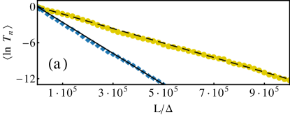
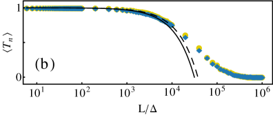
Figure 2: Illustration for how we extract the mode-specific attenuation lengths $L_{n}$ from the numerical data in the case of (a) symmetric and (b) antisymmetric waveguides (for nonsymmetric waveguides the same procedure as in (b) is used and therefore not described separately): (a) In the symmetric case where all modes localize with their own specific localization length, we fit the expression $\langle\ln T_{n}\rangle=-L/L_{n}$ (see black lines) to the mean logarithm of the numerically obtained transmission $\langle\ln T_{1}\rangle$ (yellow $\fullcircle$) and $\langle\ln T_{2}\rangle$ (blue $\blacklozenge$), shown here versus the reduced length $L/\Delta$ (for $\Delta=0.64$). (b) In the antisymmetric case we restrict ourselves to the ballistic regime, where the transmission of each mode decays along the following expression $\langle T_{n}\rangle=1-L/L_{n}$ (see black lines), which we use as a fitting curve for the mean numerically obtained transmission $\langle T_{1}\rangle$ (yellow $\fullcircle$) and $\langle T_{2}\rangle$ (blue $\blacklozenge$), shown here versus the reduced length $L/\Delta$ (for $\Delta=1.53$). An automated fitting procedure yields mode-specific attenuation lengths $L_{n}$ which show excellent agreement with our analytical estimates (see below). In the above figures, $\sigma\approx 0.01$ and $k=2.55/\pi$ have been employed, respectively.

Following this analysis we extract from the disorder-averaged transmission the numerical values for $L^{(b)}_{nn}$ through the identity $\langle\ln T_{nn}\rangle\!=\!-L/L^{(b)}_{nn}$ and compare it to the corresponding analytical predictions in equations (17) and (18). The corresponding results for $1/L^{(b)}_{nn}$ as a function of $\Delta$ are shown in figure 3(a). We also plot the theoretical predictions given by equations (17) and (18), respectively, as well as the AGS terms $1/L^{(b,AGS)}_{11}$ and $1/L^{(b,AGS)}_{22}$ alone. The agreement we find between the AGS terms and the numerical calculations is already remarkably good for most of the chosen parameters, such that the SGS contributions can be easily identified to be dominant at those specific parameter values where deviations from the AGS predictions occur (see vertical arrows in figure 3(a)). In full agreement with our theoretical analysis, we find that the values of the step width $\Delta$ where this happens are determined by the resonance condition $2k_{n}\Delta=2\pi M$ (with $M$ an integer), that we identified already earlier as those points where the contribution of the AGS terms vanishes while the SGS terms are maximal. Note that this condition leads to different resonance values for each of the two modes with $n=1,2$,

$$\Delta=\frac{\pi}{k_{n}}M=\frac{\pi}{\sqrt{k^{2}-(n\pi/d)^{2}}}M\approx\cases{\begin{array}[]{l}0.426~{}M\qquad n=1\ ,\\ 0.632~{}M\qquad n=2\ .\end{array}}$$ (19)

At these well-defined values we not only find that the theory solely based on the AGS terms deviates from the numerics (see figure 3(b)), but that the additional SGS terms fill the missing gaps in the theory very well in terms of resonant contributions to the inverse attenuation lengths $1/L_{nn}$ (see figure 3(a)). Since maxima in the inverse attenuation length correspond to maxima in the reflection (i.e., minima in the transmission) we may thus conclude that the SGS mechanism leads to reflection resonances in the systems under study. While these resonances are clearly discernible already in the symmetric waveguides, we will find that they are even more pronounced in the antisymmetric waveguides that we investigate in the next section.

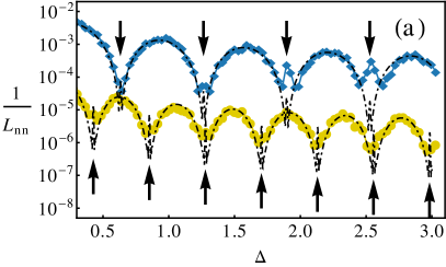
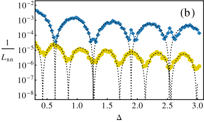
Figure 3: Inverse partial attenuation length $1/L_{nn}$ versus step width $\Delta$, as obtained numerically for two-mode symmetric waveguides. $1/L_{11}$ (yellow $\fullcircle$) and $1/L_{22}$ (blue $\blacklozenge$) are shown. (a) Comparison with the analytical expressions (17) and (18) (both — $\cdot$ —) including both the AGS and the SGS terms. Note the very good agreement which we find between the numerical data and the analytical theory, in particular also for those resonant values $2k_{n}\Delta=2\pi M$ where the SGS contributions dominate (marked by arrows). Panel (b) shows the AGS predictions alone, i.e., when the SGS mechanism is omitted (both ${\mathinner{\cdotp\cdotp\cdotp\cdotp\cdotp\cdotp}}$). For all data shown the following parameter values were used: $\rho=0.01$ , $N_{\mathrm{eff}}=25$, $\sigma\approx 0.01$ and $k=2.55/\pi$ .

5.2 Antisymmetric profiles

In the case of antisymmetric waveguide profiles we have $\xi_{\downarrow}(x)=\xi_{\uparrow}(x)$, i.e., the waveguide width is constant throughout the waveguide (see figure 1). The situation is more complicated than in symmetric waveguides as inter-mode scattering is allowed here. A proper description of transmission thus has to incorporate both the intra- and the inter-mode scattering contributions. For mode-specific values of the transmission we again have to ask which scattering events contribute: consider, e.g., the transmission of a mode into itself, $T_{nn}$. In a perturbative treatment this quantity is determined by all scattering mechanisms that scatter the incoming mode $n$ into the other mode or reverse its direction of propagation. This happens both through forward-scattering from mode $n$ into the second available mode $n^{\prime}\neq n$ as well as through backward scattering into any of the two modes $n^{\prime}=1,2$. The attenuation length extracted from the transmission $T_{nn}$ thus has to be compared to the predictions for the attenuation length $L_{nn}$ which is given as $1/L_{nn}=1/L^{(f)}_{n\neq n^{\prime}}+1/L^{(b)}_{nn}+1/L^{(b)}_{n\neq n^{\prime}}$. To be specific, we find

$$\frac{1}{L_{11}}=16\pi^{4}\frac{\sigma^{2}}{d^{6}}\frac{1}{k_{1}k_{2}}\bigg{[}W(k_{1}+k_{2})+W(k_{1}-k_{2})\bigg{]}+\frac{\pi^{4}}{2}\frac{\sigma^{4}}{d^{4}}\frac{1}{k_{1}^{2}}S(2k_{1})\ ,$$ (20)

$$\frac{1}{L_{22}}=16\pi^{4}\frac{\sigma^{2}}{d^{6}}\frac{1}{k_{1}k_{2}}\bigg{[}W(k_{1}+k_{2})+W(k_{1}-k_{2})\bigg{]}+8\pi^{4}\frac{\sigma^{4}}{d^{4}}\frac{1}{k_{2}^{2}}S(2k_{2})\ .$$ (21)

The remaining question at this point is how to extract the attenuation lengths $L_{nn}$ from the numerical data for $T_{nn}$ when modes do not just localize as in the symmetric case. In the presence of inter-mode scattering, the wave injected into a disordered waveguide first propagates ballistically, then scatters diffusively and eventually localizes at very long waveguide lengths. For the two-mode waveguide considered here the diffusive regime is, however, not well-pronounced such that the crossover region between ballistic scattering and localization is comparatively narrow. Since, additionally, in the localized regime always the mode with the higher localization length $\xi$ dominates [20], extracting mode-specific attenuation lengths is best achieved in the ballistic regime where the transmission decreases linearly with the system length $L$, $\langle T_{nn}\rangle\approx 1-L/L_{nn}$. We will use this relation to extract the attenuation lengths $L_{nn}$ from the disorder-averaged numerical transmission values $\langle T_{nn}\rangle$ in the ballistic regime. In practice, we use the criterion $\langle T_{nn}\rangle\in[0.9,1]$ to ensure that the requirement of ballistic transport is satisfied (see figure 2(b)).

Figure 4 shows the numerically obtained results for $1/L_{nn}$, including a comparison with the predictions from equations (20) and (21). In panel (a), both modes are displayed, with yellow full circles corresponding to $n=1$ and blue diamonds to $n=2$, respectively. In the case of antisymmetric waveguides a direct comparison of the numerical results for the two different modes reveals immediately where the SGS mechanism is at work (see figure 4(a)): Since the terms in equations (20) and (21) associated with the AGS mechanism are identical for $1/L_{11}$ and $1/L_{22}$, any difference between the two attenuation lengths can be expected to be due to the SGS mechanism. The numerical results reveal that around $\Delta\approx 2.5$ an extended region opens up in which the two modes decouple and their attenuation lengths are significantly different. To clarify whether this decoupling is, indeed, due to the SGS mechanism, we compare the numerical results with the corresponding analytical predictions in figures 4(b,c). The agreement we obtain is, again, excellent, allowing us to identify the contributions of the SGS mechanism in detail. First of all, we find that the decoupling of modes is, indeed, due to the SGS mechanism as it is accurately reproduced when the SGS terms are included. Secondly, the theoretical analysis also predicts that the SGS terms should give rise to small resonant enhancements of the inverse attentuation length at the resonant values $2k_{n}\Delta=2\pi M$ (see arrows in figures 4(b,c)). Also these predictions are very well reproduced by the numerical data.

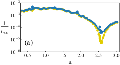
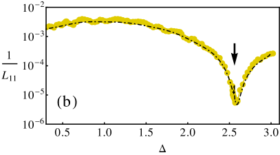
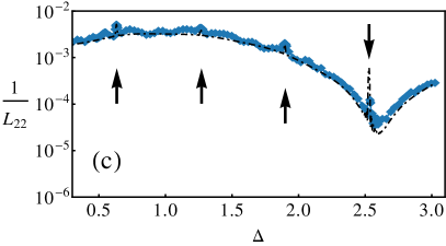
Figure 4: (a) Inverse partial attenuation length $1/L_{nn}$ versus the step width $\Delta$, as obtained numerically for two-mode antisymmetric waveguides, with $1/L_{11}$ (yellow $\fullcircle$) and $1/L_{22}$ (blue $\blacklozenge$). We find very good agreement with the analytical expressions (20) and (21) that are included as dotdashed lines (— $\cdot$ —) in panel (b) and (c), respectively (with $\rho=0.03$, $N_{\mathrm{eff}}=25$, $\sigma\approx 0.01$ and $k=2.55/\pi$). Arrows mark resonant values $2k_{n}\Delta=2\pi M$ which indicate locally dominating SGS contributions.

To corroborate the consistency of our above arguments on forward- and backward-scattering contributions we also investigated the total mode transmissions $T_{n}=\sum^{N_{d}}_{n^{\prime}}|t_{nn^{\prime}}|^{2}$, which are now different from the mode-to-mode transmissions $T_{nm}$ due to inter-mode scattering. In the ballistic regime the $T_{n}$ should be determined by backward-scattering alone, since forward-scattering just redistributes the flux which is incoming in one mode over all available right-moving modes. Since, however, the right-moving modes are summed over in the expression for $T_{n}$, any influence of forward-scattering drops out in our perturbative treatment. Only when taking into account higher-order forward/backward-scattering events (as in the diffusive or localized regime) the influence of forward-scattering should be noticeable also on the $T_{n}$. In the ballistic regime, however, we should have $\langle T_{n}\rangle\approx 1-L/L_{n}$, with $1/L_{n}=1/L^{(b)}_{nn\phantom{(}}+1/L^{(b)}_{n\neq n^{\prime}}$ such that the mode-specific attentuation lengths read as follows,

$$\frac{1}{L_{1}}=16\pi^{4}\frac{\sigma^{2}}{d^{6}}\frac{W(k_{1}+k_{2})}{k_{1}k_{2}}+\frac{\pi^{4}}{2}\frac{\sigma^{4}}{d^{4}}\frac{S(2k_{1})}{k_{1}^{2}}\ ,$$ (22)

$$\frac{1}{L_{2}}=16\pi^{4}\frac{\sigma^{2}}{d^{6}}\frac{W(k_{1}+k_{2})}{k_{1}k_{2}}+8\pi^{4}\frac{\sigma^{4}}{d^{4}}\frac{S(2k_{2})}{k_{2}^{2}}\ .$$ (23)

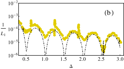
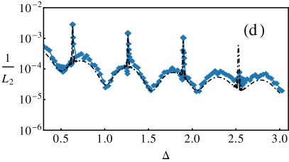
Figure 5: Inverse partial attenuation length $1/L_{n}$ versus step width $\Delta$, as obtained numerically for two-mode antisymmetric waveguides ($\rho=0.03$, $N_{\mathrm{eff}}=25$, $\sigma\approx 0.01$ and $k=2.55/\pi$). Top row: The numerical results for $1/L_{1}$ (yellow $\fullcircle$) are compared in (a) with the AGS (${\mathinner{\cdotp\cdotp\cdotp\cdotp\cdotp\cdotp}}$) and SGS (-  -  -  -) terms of equation (22) plotted separately. In (b) both scattering mechanisms are combined (— $\cdot$ —). Bottom row: Numerical values for $1/L_{2}$ (blue $\blacklozenge$) are compared in (c) with the AGS (${\mathinner{\cdotp\cdotp\cdotp\cdotp\cdotp\cdotp}}$) and SGS (-  -  -  -) terms of equation (23) plotted separately. In (d) both scattering mechanisms are combined (— $\cdot$ —). We find a quantitative agreement with the predictions for $1/L_{2}$ (panel (d)), while a sizeable discrepancy is observed between numerics and analytical curves for the first mode in (b).

To extract the corresponding attenuation lengths $L_{n}$ from our numerics, we use $\langle T_{n}\rangle\approx 1-L/L_{n}$ as a prescription to obtain $L_{n}$ in the ballistic regime, characterized by $\langle T_{n}\rangle\in[0.9,1]$. The agreement which we find between the predictions for $1/L_{n}$ and our numerical results is, in parts, remarkably good (see figure 5). A comparison with the expression for $1/L_{2}^{\phantom{(b)}}=1/L_{2}^{(b,AGS)}+1/L_{2}^{(b,SGS)}$ in figure 5(d) reveals an excellent agreement between theory and simulation. With the help of figure 5(c), it can be understood that the SGS mechanism contributes by way of two distinct effects: most obviously, we obtain peaks indicating enhanced resonant back-scattering in our system for $2k_{2}\Delta=2\pi M$, with $M$ integer. Note that these peaks in $1/L_{2}$ lead to back-scattering lengths which are about one order of magnitude larger than the (conventional) AGS background. The SGS mechanism can, however, also be identified as a finite contribution to the inverse scattering length at values $(k_{1}+k_{2})\Delta=2\pi M^{\prime}$, exactly where the AGS term in equation (23) vanishes. It is therefore the SGS mechanism which prevents a perfect transparency of the waveguide.

When comparing the first mode data to equation (22), we find that the numerical curve cannot be fully reproduced by the corresponding analytical expression for $1/L_{1}$ (see figure 5(b)). While the AGS contribution $1/L_{1}^{(b,AGS)}$ is identical to $1/L_{2}^{(b,AGS)}$ in antisymmetric waveguides, the SGS contribution $1/L_{1}^{(b,SGS)}$ is a factor $16$ smaller (see figure 5(a)). How can this be reconciled with the numerical finding that $1/L_{1}$ and $1/L_{2}$ are mostly equal?

We suspect higher-order terms in scattering to be responsible for these deviations which go beyond the first order nature of the underlying theory, where the incident wave is assumed to scatter only once before leaving the scattering region. Our aim in the following will be to include such higher-order contributions based on the knowledge of the first-order scattering lengths. Consider here, e.g., the scattering length of the first mode, $L_{1}$, which, as we have assumed so far, is attenuated by back-scattering from the first mode into the first ($L^{(b)}_{11}$) and into the second mode ($L^{(b)}_{12}$), respectively. The next higher order contribution would be given by forward scattering into the second mode (governed by $L^{(f)}_{12}$), followed by back-scattering from the second mode into the first ($L^{(b)}_{21}$) or into the second mode ($L^{(b)}_{22}$).

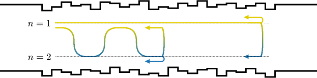
Figure 6: Illustration of scattering processes of different order. Two processes are shown that attenuate the forward moving first mode, $n=1$. One process is of first order and consists just of a single back-scattering event from the first mode into any of the two backward-moving modes. However, since in the case we consider, forward-scattering $1\leftrightarrow 2$ is dominant as compared to backscattering, it is much more likely that the first mode undergoes multiple scattering events in forward direction before backscattering occurs. Such terms can thus yield a sizeable contribution although they formally are of higher-order in the number of scattering events which they undergo.

Based on the magnitude of the involved scattering lengths the forward-scattering $1\leftrightarrow 2$ occurs much more frequently than a back-scattering event, i.e., the propagating wave undergoes forward scattering multiple times before it is backscattered (see figure 6). Consequently, the modes can be assumed to be almost equally distributed between mode $1$ or $2$ before back-scattering occurs. As a result, the back-scattering contribution should also be composed of both modes in equal shares. Since the forward-scattering occurs in series, the back-scattering in parallel, this translates into an additional effective second order term for the inverse scattering length,

$$\frac{1}{L^{(2,\mathrm{eff})}}=\frac{1}{L^{(f)}+\frac{1}{\frac{1}{2}\left(\frac{1}{L^{(b)}_{21}}+\frac{1}{L^{(b)}_{22}}+\frac{1}{L^{(b)}_{12}}+\frac{1}{L^{(b)}_{11}}\right)}}\ ,$$ (24)

with $L^{(f)}\equiv L^{(f)}_{12}=L^{(f)}_{21}$. Equation (24) represents a simple qualitative estimate of second order contributions to the inverse scattering lengths, and we expect that this expression can be made more quantitative by employing a full-fledged diagrammatic theory. Note that this correction term does not feature an explicit mode dependence since the redistribution of the flux is the same for both propagating modes.

Based on the above, the total inverse scattering lengths can be written as the sum of the following contributions,

$$\frac{1}{L_{n}^{\phantom{(b)}}} = \frac{1}{L^{(b)}_{nn}}+\frac{1}{L^{(b)}_{nn^{\prime}\neq n}}+\frac{1}{L^{(2,\mathrm{eff})}_{\phantom{n}}}\ ,$$ (25)

$$= \frac{1}{L_{n}^{(1)}}+\frac{1}{L^{(2,\mathrm{eff})}_{\phantom{n}}}\ ,$$

where the superscripts $(i)$ denote the order of the contribution. A comparison of this result with the numerical data is shown in figure 7, yielding much better agreement than without the second-order contributions. In particular, we find (see figure 7(a)) that incorporating the new effective scattering length $1/L^{(2,\mathrm{eff})}$ resolves the discrepancy we found earlier for the inverse attenuation length of the first mode, $1/L_{1}$. This result now also allows us to understand the similarity between the numerical data for $1/L_{1}$ and $1/L_{2}$ while the first-order SGS contributions are very different for these two modes: the reason is apparently the strong intermode coupling induced by efficient forward-scattering $L^{(f)}$ which lets the inverse attenuation length of the first mode $1/L_{1}$ inherit the behaviour of the second mode $1/L_{2}$.

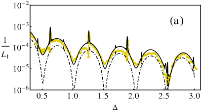
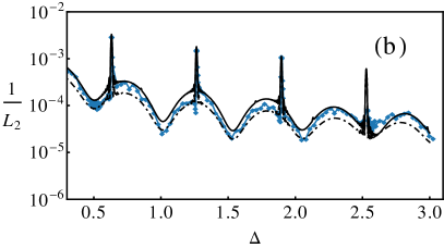
Figure 7: Inverse partial attenuation length $1/L_{n}$ versus step width $\Delta$, as obtained numerically for two-mode antisymmetric waveguides ($\rho=0.03$, $N_{\mathrm{eff}}=25$, $\sigma\approx 0.01$ and $k=2.55/\pi$ ). The inverse attenuation lengths are shown in (a) for the first mode, $1/L_{1}$ (yellow $\fullcircle$) and in (b) for the second mode $1/L_{2}$ (blue $\blacklozenge$). The analytical curves are displayed without (— $\cdot$ —) and including (——) second order corrections of equation (24). Note the quantitative agreement that is achieved through the inclusion of higher-order scattering terms.

Correspondingly, the reason for the decoupling between the modes in figure 7 at around $\Delta\approx 2.5$ can also now be identified: in this parameter window the intermode scattering strength is strongly reduced, allowing the different attenuation lengths to maintain their mode-specific values. Everywhere else (outside this parameter window) the behaviour of $1/L_{1}$ is governed by $1/L_{2}$.

5.3 Nonsymmetric profiles

Nonsymmetric waveguides represent the most general case for waveguide symmetries since, in contrast to the previous sections, both boundaries are not restricted by any symmetry requirement, i.e., we have $\xi_{\uparrow}(x)\neq\xi_{\downarrow}(x)$. Turning at first to the partial attenuation lengths, table 1 and equations (14) and (15) allow us to put forward the corresponding expressions for $1/L_{nn}=1/L^{(f)}_{n\neq n^{\prime}}+1/L^{(b)}_{nn}+1/L^{(b)}_{n\neq n^{\prime}}$, which are given by

$$\frac{1}{L_{11}}=2\pi^{4}\frac{\sigma^{2}}{d^{6}}\frac{1}{k_{1}^{2}}W(2k_{1})+8\pi^{4}\frac{\sigma^{2}}{d^{6}}\frac{1}{k_{1}k_{2}}\bigg{[}W(k_{1}+k_{2})+W(k_{1}-k_{2})\bigg{]}$$

$$\qquad~{}+20\frac{\sigma^{4}}{d^{4}}\frac{1}{k_{1}^{2}}S(2k_{1})+\frac{(9+6\pi^{2}+10\pi^{4})}{72\pi^{4}}\frac{\sigma^{2}}{d^{6}}\frac{1}{k_{1}k_{2}}\bigg{[}S(k_{1}+k_{2})+S(k_{1}-k_{2})\bigg{]}\ ,$$ (26)

$$\frac{1}{L_{22}}=32\pi^{4}\frac{\sigma^{2}}{d^{6}}\frac{1}{k_{1}^{2}}W(2k_{2})+8\pi^{4}\frac{\sigma^{2}}{d^{6}}\frac{1}{k_{1}k_{2}}\bigg{[}W(k_{1}+k_{2})+W(k_{1}-k_{2})\bigg{]}$$

$$\qquad~{}+20\frac{\sigma^{4}}{d^{4}}\frac{1}{k_{1}^{2}}S(2k_{2})+\frac{(9+24\pi^{2}+160\pi^{4})}{72\pi^{4}}\frac{\sigma^{2}}{d^{6}}\frac{1}{k_{1}k_{2}}\bigg{[}S(k_{1}+k_{2})+S(k_{1}-k_{2})\bigg{]}\ .$$ (27)

We can also immediately write down the corresponding total scattering lengths $1/L_{n}=1/L^{(b)}_{nn}+1/L^{(b)}_{n\neq n^{\prime}}$, where forward-scattering, i.e., $W(k_{1}-k_{2})$ and $S(k_{1}-k_{2})$, is not considered since it does not attenuate the total transmission $T_{n}$ of the corresponding mode,

$$\frac{1}{L_{1}}=2\pi^{4}\frac{\sigma^{2}}{d^{6}}\frac{1}{k_{1}^{2}}W(2k_{1})+8\pi^{4}\frac{\sigma^{2}}{d^{6}}\frac{1}{k_{1}k_{2}}W(k_{1}+k_{2})$$

$$\qquad~{}+20\frac{\sigma^{4}}{d^{4}}\frac{1}{k_{1}^{2}}S(2k_{1})+\frac{(9+6\pi^{2}+10\pi^{4})}{72\pi^{4}}\frac{\sigma^{2}}{d^{6}}\frac{1}{k_{1}k_{2}}S(k_{1}+k_{2})\ ,$$ (28)

$$\frac{1}{L_{2}}=32\pi^{4}\frac{\sigma^{2}}{d^{6}}\frac{1}{k_{1}^{2}}W(2k_{2})+8\pi^{4}\frac{\sigma^{2}}{d^{6}}\frac{1}{k_{1}k_{2}}W(k_{1}+k_{2})$$

$$\qquad+20\frac{\sigma^{4}}{d^{4}}\frac{1}{k_{1}^{2}}S(2k_{2})+\frac{(9+24\pi^{2}+160\pi^{4})}{72\pi^{4}}\frac{\sigma^{2}}{d^{6}}\frac{1}{k_{1}k_{2}}S(k_{1}+k_{2})\ .$$ (29)

As can be seen from these equations for $1/L_{n}$ and $1/L_{nn}$, intra- and intermode as well as the AGS and the SGS scattering lengths now all contribute to the scattering process, in contrast to symmetric or antisymmetric waveguides where the coefficient matrices $A_{nn^{\prime}}$ and $B_{nn^{\prime}}$ from table 1 feature zeros at symmetry-specific entries. This fact underlines the role of nonsymmetric waveguides as the most general case to study in surface-corrugated systems.

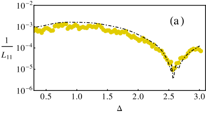
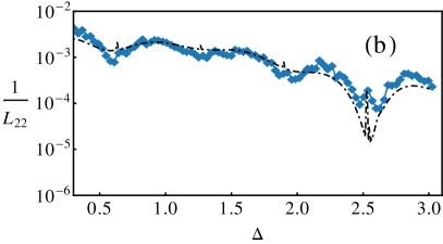
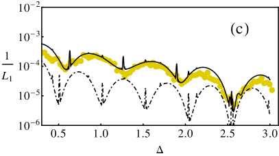
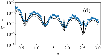
Figure 8: Inverse partial attenuation length $1/L_{nn}$ versus step width $\Delta$, as obtained numerically for two-mode nonsymmetric waveguides ($\rho=0.03$, $N_{\mathrm{eff}}=25$, $\sigma\approx 0.01$ and $k=2.55/\pi$ ). Top row: The numerical results for (a) $1/L_{11}$ (yellow $\fullcircle$) and (b) $1/L_{22}$ (blue $\blacklozenge$) are shown. The corresponding analytical expressions (26) and (27) are shown in black (— $\cdot$ —), indicating very good agreement with the numerical data. Bottom row: Here the numerical data for (c) $1/L_{1}$ (yellow $\fullcircle$) and (d) $1/L_{2}$ (blue $\blacklozenge$) are compared with the corresponding analytical terms without (— $\cdot$ —) and including (——) second order corrections. Even though nonsymmetric waveguides represent the most general of waveguide symmetries, we find a remarkably good agreement with our numerics.

For comparison with the numerical data we determine the quantities $1/L_{nn}$ and $1/L_{n}$ by means of a fit to the transmission in the ballistic regime, $\langle T_{nn}\rangle\approx 1-L/L_{nn}$ and $\langle T_{n}\rangle\approx 1-L/L_{n}$, in complete analogy to antisymmetric waveguides in the preceding section. Figure 8 shows a comparison between numerics and theory for nonsymmetric two-mode waveguides. Concentrating at first on $1/L_{nn}$ (first row in figure 8), we note that we find very good agreement between the theoretical and the numerical curves for both the first and the second mode. Similar to the corresponding results in antisymmetric waveguides, a peak at $\Delta\approx 2.5$ is clearly visible for $1/L_{22}$ and, more hidden, also in $1/L_{11}$. The other peaks emerging in the analytical expression for $1/L_{22}$ can also be found in our numerical data (figure 8(b)), albeit slightly more concealed than in the previous section. The positions of these resonances can again be determined from the resonance condition in equation (19).

Turning to the assessment of our results for $1/L_{n}$ we can now, with the knowledge from the last section, also take into account higher-order scattering contributions given by equation (24). Figures 8(c-d) show a comparison of the analytical expressions for the attenuation lengths $1/L_{n}$ with the numerical data. Note that here we also include the first order predictions as dotdashed lines. As found before in antisymmetric two-mode waveguides, $1/L_{2}$ is already captured very well by equation (29). The arc-structure driven by the AG scattering mechanism shows again a remarkable agreement with the numerical curve, the same is true at resonant points where we find dominating contributions of the SGS mechanism. As before, a more elaborate argument incorporating second-order terms in the scattering is needed for explaining the behaviour of $1/L_{1}$ (figure 8(c)). Taking only first-order expressions from equation (28) into account results in theoretical predictions which deviate from our numerical data by about one order of magnitude. Moreover, the period of the oscillations in $1/L_{1}$ does not seem to coincide with the analytical predictions. Only after allowing for higher-order terms in $1/L_{n}$, i.e., where forward-scattering followed by back-scattering is taken into account by employing equation (24), an agreement can be reestablished (figure 8(c) solid line).

Note that the reflection resonances which we observe for nonsymmetric and symmetric waveguides are not as pronounced as in the case of antisymmetric waveguides. This can be understood by the fact that the cross-section of an antisymmetric waveguide remains constant throughout the entire waveguide length such that also the wavenumber $k_{x}$ does not change in the course of propagation. As a consequence, the resonance condition $k\Delta=2\pi M$, with M integer, can be fulfilled very accurately in antisymmetric waveguides, while for waveguides with different symmetries the resonance condition is fulfilled only on average.

6 Summary

In summary, we have investigated waveguides with a step-like surface disorder supporting two propagating modes. Our study reveals a resonant enhancement of wave reflection in these systems, an effect which has, to the best of our knowledge, not yet been observed earlier, despite the popularity of the employed waveguide model. To manifest this effect we performed extensive numerical calculations using a waveguide model with symmetric, antisymmetric and nonsymmetric random profiles, respectively. We compare our numerical findings to a recently proposed surface scattering theory [33, 34] which we extend to include higher-order scattering processes as well as to account for the limited resolution with which a scattering wave is sensitive to the surface disorder. We find very good agreement with this new theoretical framework and can thereby associate the origin of the reflection resonances with a higher-order term in the weak disorder expansion of the attenuation lengths. A detailed derivation of this so-called “square gradient scattering” term is put forward, which, for the systems we consider, results in a fully analytical expression. We show that this previously neglected contribution is very robust and survives ensemble-averaging of the surface roughness. At the resonance conditions, $k_{x}\Delta=2\pi M$, with $M$ integer, we find up to an order-of-magnitude enhancements of the reflection. Not only do our results constitute the first evidence of these resonances in waveguides, but they also provide the first unambiguous signatures of the square-gradient scattering mechanism in waveguides with arbitrary symmetries. The very good agreement which we find between numerical and analytical results provides a solid basis for a general understanding of wave transmission through waveguides with surface roughness. This knowledge may be particularly important in view of experimental possibilities to engineer the transmission characteristics of waveguides through their surface profiles [42, 43].

Appendix

A.1 Step-profile $\xi(x)$

In order to describe an effective smoothing of a step-like waveguide boundary due to a finite resolution capacity of the propagating wave, we consider a profile $\xi(x)$ which consists of $2N+1$ steps of width $\Delta$ and random heights $\alpha_{n}$ that feature zero mean and unit variance,

$$\xi(x)=\sum_{n=-N}^{N}\alpha_{n}\ \Pi_{\rho}(x-n\Delta)\ .$$ (30)

The smoothing of the steps is modelled by assuming $\Pi_{\rho}(x)$ to be the sum of two Fermi-functions $F_{\rho}(x)$,

$$\Pi_{\rho}(x)=F_{\rho}(x-\Delta)-F_{\rho}(x)=\frac{1}{1+e^{(x-\Delta)/\rho}}-\frac{1}{1+e^{x/\rho}}\ ,$$ (31)

with the parameter $\rho$ controlling the smearing of the steps, corresponding to the finite resolution of the propagating wave. In the limit of $\rho\to 0$, i.e., if we assume perfect resolution, the unit box function $\Theta(x)-\Theta(x-\Delta)$ is obtained (see figure 9).

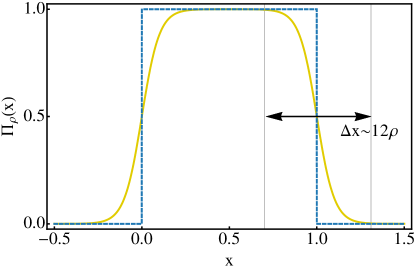
Figure 9: Plot of the smoothed step-function $\Pi_{\rho}(x)$ which represents the building block for the waveguide boundaries employed in the present paper. A comparison of $\Pi_{\rho=0.05}(x)$ (yellow ——) and $\Pi_{\rho=0}(x)$ (blue -  -  -  -) is shown, with step-width $\Delta=1$. The smeared out region $\Delta x\sim 12\rho$ used in the estimate in section 3 is indicated by grey vertical lines, as determined by the condition $|\Pi_{\rho}(\Delta\pm 6\rho)-\Pi_{0}(\Delta\pm 6\rho)|\sim 2.5\times 10^{-3}$.

A.2 Roughness-height power spectrum $W(k)$

To calculate $W(k)=\int_{-\infty}^{\infty}\exp{(-ikx^{\prime})}\langle\xi(x)\xi(x+x^{\prime})\rangle dx^{\prime}$, we employ the Wiener-Khinchin theorem [39],

$$\int_{-\infty}^{\infty}e^{-ikx^{\prime}}\langle f(x)f(x+x^{\prime})\rangle dx^{\prime}=\lim_{L\to\infty}\frac{1}{L}\left\langle\left|\tilde{f}_{L/2}(k)\right|^{2}\right\rangle\ ,$$ (32)

where $\tilde{f}_{L/2}(k)$ denotes the truncated Fourier transform,

$$\tilde{f}_{L/2}(k)\equiv\int_{-L/2}^{L/2}e^{-ikx}f(x)dx\ ,$$ (33)

which in the limit of $L\to\infty$ becomes the Fourier transform $\tilde{f}(k)\equiv\int_{-\infty}^{\infty}\exp{(-ikx)}f(x)dx$. The angular brackets $\langle\cdots\rangle$ denote ensemble averaging. For our step-profile $\xi(x)$ we obtain the following expressions,

$$\tilde{\xi}_{L/2}(k) = \sum_{n=-N}^{N}\alpha_{n}\int_{-L/2}^{L/2}\Pi_{\rho}(x-n\Delta)e^{-ikx}dx$$ (34)

$$= \sum_{n=-N}^{N}\alpha_{n}e^{-ikn\Delta}\int_{-L/2-n\Delta}^{L/2-n\Delta}\Pi_{\rho}(x)e^{-ikx}dx\ .$$

In our numerics we employ a constant number of modules but allow for a varying module width $\Delta$, the waveguide length $L$ is thus given by $L=2N\Delta$. Equation (34) therefore reads

$$\tilde{\xi}_{L/2}(k)=\sum_{n=-N}^{N}\alpha_{n}e^{-ikn\Delta}\int_{-(N+n)\Delta}^{(N-n)\Delta}\Pi_{\rho}(x)e^{-ikx}dx$$ (35)

$$\qquad\quad\approx\sum_{n=-N}^{N}\alpha_{n}e^{-ikn\Delta}\underbrace{\int_{-\infty}^{\infty}\Pi_{\rho}(x)e^{-ikx}dx}_{\tilde{\Pi}_{\rho}(k)}=\tilde{\Pi}_{\rho}(k)\sum_{n=-N}^{N}\alpha_{n}e^{-ikn\Delta}\ .$$ (36)

Here, we approximate the truncated Fourier transform in equation (35) with $\tilde{\Pi}_{\rho}(k)$, such that it is independent of the summation index $n$ and can thus be pulled it in front of the summation. For the parameters employed in the present paper this step is very well justified and only leads to a vanishingly small error.

The roughness-height power spectrum $W(k)=\lim_{L\to\infty}\frac{1}{L}\langle|\tilde{\xi}_{L/2}(k)|^{2}\rangle$ consequently becomes

$$~{}W(k)=\lim_{N\to\infty}\frac{1}{2N\Delta}\left\langle\left|\tilde{\Pi}_{\rho}(k)\sum_{n=-N}^{N}\alpha_{n}e^{-ikn\Delta}\right|^{2}\right\rangle$$

$$\qquad\quad=\frac{|\tilde{\Pi}_{\rho}(k)|^{2}}{\Delta}\lim_{N\to\infty}\frac{1}{2N}\sum_{n=-N}^{N}\sum_{m=-N}^{N}\underbrace{\left\langle\alpha_{n}\alpha_{m}\right\rangle}_{\alpha_{n}^{2}\delta_{nm}}e^{-ik(n-m)\Delta}$$

$$\qquad\quad=\frac{|\tilde{\Pi}_{\rho}(k)|^{2}}{\Delta}\lim_{N\to\infty}\frac{1}{2N}\sum_{n=-N}^{N}\alpha_{n}^{2}=\frac{1}{\Delta}|\tilde{\Pi}_{\rho}(k)|^{2}.$$ (37)

Note that we assume here that the random heights are uncorrelated, i.e., the products $\langle\alpha_{n}\alpha_{m}\rangle$ vanish for $n\neq m$. The expression $\tilde{\Pi}_{\rho}(k)$ can be calculated analytically,

$$\tilde{\Pi}_{\rho}(k) = \int_{-\infty}^{\infty}e^{-ikx}\left(F_{\rho}\left(x-\Delta\right)-F_{\rho}\left(x\right)\right)dx$$ (38)

$$= \underbrace{\tilde{F}_{\rho}(k)}_{\left(i\frac{\pi\rho}{\sinh{(\pi k\rho)}}+\pi\delta(k)\right)}\cdot\underbrace{(e^{-ik\Delta}-1)}_{\left(-2ie^{-ik\Delta/2}\sin{(k\Delta/2)}\right)}\ .$$

Since we evaluate $W(k)$ at finite $k$ values we omit the delta function $\delta(k)$ in the following, yielding finally

$$W(k)=\frac{1}{\Delta}\frac{4\pi^{2}\rho^{2}}{\sinh^{2}{(\pi k\rho)}}\sin^{2}{(k\Delta/2)}\ .$$ (39)

A.3 Square-gradient power spectrum $S(k)$

For the squared gradient of $\xi(x)$ we have

$$\xi^{\prime}(x)^{2}=\sum_{n=-N}^{N}\sum_{m=-N}^{N}\alpha_{n}\alpha_{m}\Pi^{\prime}_{\rho}(x-n\Delta)\Pi^{\prime}_{\rho}(x-m\Delta)\ .$$ (40)

Under the assumption that the smearing parameter $\rho$ fulfils the relation $\rho\lesssim\Delta/12$, the product $\Pi^{\prime}_{\rho}(x-n\Delta)\Pi^{\prime}_{\rho}(x-m\Delta)$ is only finite if $n=m$, $n=m+1$ and $n=m-1$, respectively, i.e.,

$$\Pi^{\prime}_{\rho}(x-n\Delta)\Pi^{\prime}_{\rho}(x-m\Delta)\approx\delta_{n,m}F^{\prime}_{\rho}\big{(}x-(n+1)\Delta\big{)}F^{\prime}_{\rho}\big{(}x-(m+1)\Delta\big{)}$$

$$\qquad\qquad\qquad+~{}\delta_{n,m}F^{\prime}_{\rho}\big{(}x-n\Delta\big{)}F^{\prime}_{\rho}\big{(}x-m\Delta\big{)}$$

$$\qquad\qquad\qquad~{}-\delta_{n-1,m}F^{\prime}_{\rho}\left(x-n\Delta\right)F^{\prime}_{\rho}\big{(}x-(m+1)\Delta\big{)}$$

$$\qquad\qquad\qquad~{}~{}-\delta_{n+1,m}F^{\prime}_{\rho}\big{(}x-(n+1)\Delta\big{)}F^{\prime}_{\rho}\left(x-m\Delta\right)\ ,$$ (41)

resulting in

$$\xi^{\prime}(x)^{2}\approx\sum_{n=-N}^{N}\alpha_{n}^{2}\bigg{[}F^{\prime 2}_{\rho}\left(x-(n+1)\Delta\right)+F^{\prime 2}_{\rho}\left(x-n\Delta\right)\bigg{]}$$

$$\qquad\qquad-\alpha_{n}\alpha_{n+1}F^{\prime 2}_{\rho}\left(x-(n+1)\Delta\right)-\alpha_{n}\alpha_{n-1}F^{\prime 2}_{\rho}\left(x-n\Delta\right)\ .$$ (42)

To calculate the square-gradient power spectrum $S(k)$ we have, with $V(x)=\xi^{\prime 2}(x)-\langle\xi^{\prime 2}(x)\rangle$,

$$S(k) = \frac{1}{2}\int_{-\infty}^{\infty}e^{-ikx^{\prime}}\langle V(x)V(x+x^{\prime})\rangle dx^{\prime}$$ (43)

$$= \frac{1}{2}\int_{-\infty}^{\infty}e^{-ikx^{\prime}}\langle\xi^{\prime 2}(x)\xi^{\prime 2}(x+x^{\prime})\rangle dx^{\prime}-\pi\langle\xi^{\prime 2}(x)\rangle^{2}\delta(k)\ ,$$

where we again employ the Wiener-Khinchin theorem equation (32). Identifying $\xi^{\prime 2}(x)$ with $f(x)$, we have

$$\tilde{f}(k)=\int_{-\infty}^{\infty}e^{-ikx}\xi^{\prime 2}(x)dx$$

$$\qquad=\underbrace{\int_{-\infty}^{\infty}e^{-ikx}F_{\rho}^{\prime 2}(x)dx}_{\frac{1}{6}k\pi\frac{(1+k^{2}\rho^{2})}{\sinh{(\pi k\rho)}}}\sum_{n=-N}^{N}e^{-ikn\Delta}\Bigg{[}\alpha_{n}^{2}\left(1+e^{-ik\Delta}\right)-\alpha_{n}\alpha_{n+1}e^{-ik\Delta}-\alpha_{n}\alpha_{n-1}\Bigg{]}$$ (44)

In analogy to the reasoning for equation (39), we neglect the additional contribution at $k=0$. The square-gradient roughness spectrum $S(k)=\lim_{L\to\infty}\frac{1}{L}\langle|\tilde{f}_{L/2}(k)|^{2}\rangle$ thus becomes

$$S(k)=\frac{1}{\Delta}\frac{k^{2}\pi^{2}}{72}\frac{\left(1+k^{2}\rho^{2}\right)^{2}}{\sinh^{2}{(\pi k\rho)}}\Omega(k\Delta)\ ,$$ (45)

with the auxiliary function $\Omega(x)$,

$$\Omega(x)=\lim_{N\to\infty}\frac{1}{2N}\left\langle\left|\sum_{n=-N}^{N}e^{-inx}\bigg{[}\alpha_{n}^{2}\left(1+e^{-ix}\right)-\alpha_{n}\alpha_{n+1}e^{-ix}-\alpha_{n}\alpha_{n-1}\bigg{]}\right|^{2}\right\rangle$$

$$\qquad=\lim_{N\to\infty}\left[\frac{4}{5}\left(1+\frac{1}{2N}\right)\bigg{(}7+2\cos{(x)}\bigg{)}+2\bigg{(}1+\cos{(x)}\bigg{)}\frac{1}{2N}\frac{\sin^{2}{\left[(N+\frac{1}{2})x\right]}}{\sin^{2}{(x/2)}}\right]\ .$$ (46)

References

References

- [1] DeSanto J A and Brown G S Analytical techniques for multiple scattering from rough surfaces in Progress in optics, Vol. 23, edited by E. Wolf (Elsevier, Amsterdam, 1986) Chap. 1, pp. 1.62
- [2] Bass F G and Fuks I M Wave Scattering from Statistically Rough Surfaces (Pergamon, New York, 1979)
- [3] Maradudin A Light Scattering and Nanoscale Surface Roughness (Springer, New York, 2007)
- [4] Tsang L and Kong J A Scattering of electromagnetic waves: Advanced topics (Wiley, New York, 2001).
- [5] Medwin H and Clay C S Fundamentals of Acoustic Oceanography (Academic Press, San Diego, 1998)
- [6] Li C, Kattawar G W and Yang P 2004 JQSRT 89 123
- [7] Gan L and Li Z 2012 Front. Optoelectron. 5 21; Roberts P, Couny F, Sabert H, Mangan B, Birks T, Knight J and Russell P 2005 Opt. Express 13 7779
- [8] Chaikina E I, Stepanov S, Navarrete A G, Méndez E R and Leskova T A 2005 Phys. Rev. B 71 085419; Phan-Huy M-C, Moison J-M, Levenson J A, Richard S, Mélin G, Douay M and Quiquempois J 2009 J. Lightwave Technol. 27 1597
- [9] Maker A J and Armani A M 2011 Opt. Lett. 36 3729; Lee K K, Lim D R, Luan H-C, Agarwal A, Foresi J and Kimerling L C 2000 Appl. Phys. Lett. 77 1617
- [10] Zayats A V, Smolyaninov I I and Maradudin A A 2005 Phys. Rep. 408 131
- [11] Structured Surfaces as Optical Metamaterials edited by Maradudin A A (Cambridge University Press, Cambridge, New York, 2011)
- [12] Fishman G and Calecki D 1989 Phys. Rev. Lett. 62 1302; Mayerovich A E and Stepaniants A 1999 Phys. Rev. B 60 9129
- [13] Chopra K L Thin film phenomena (McGraw-Hill, New York, 1969)
- [14] Makarov N M, Moroz A V and Yampol’skii V A 1995 Phys. Rev. B 52 6087; Meyerovich A E and Stepaniants S 1994 Phys. Rev. Lett. 73 316; Meyerovich A E and Stepaniants S 1995 Phys. Rev. B 51 17116; Stepaniants A, Sarkisov D, and Meyerovich A E 1999 J. Low Temp. Phys. 114 371; Meyerovich A E and Stepaniants S 2000 J. Phys. Condens. Matter 12 5575
- [15] Zhang S, Levy P M and Fert A 1992 Phys. Rev. B 45 8689; Gámiz F, Roldán J B, López-Villanueva J A, Cartujo-Cassinello P and Carceller J E 1999 Appl. Phys. Lett. 86 6854
- [16] Han M Y, Özyilmaz B, Zhang Y and Kim P 2007 Phys. Rev. Lett. 98 206805; Mucciolo E R, Castro Neto A H and Lewenkopf C H 2009 Phys. Rev. B 79 075407; Evaldsson M, Zozoulenko V, Xu H and Heinzel T 2008 Phys. Rev. B 78 161407
- [17] Libisch F, Rotter S and Burgdörfer J 2012 New J. Phys. 14 123006
- [18] Huber T E, Nikolaeva A, Gitsu D, Konopko L and Graf M J 2009 J. Appl. Phys. 104 123704
- [19] Akguc G B and Gong J 2008 Phys. Rev. B 78 115317
- [20] Feist J, Bäcker A, Ketzmerick R, Rotter S, Huckestein B and Burgdörfer J 2006 Phys. Rev. Lett. 97 116804; Feist J, Bäcker A, Ketzmerick R, Burgdörfer J, and Rotter S 2009 Phys. Rev. B 80 245322
- [21] Ferry D K, Goodnick S M and Bird J P Transport in Nanostructures, 2nd ed. (Cambridge University Press, Cambridge, UK, 2009)
- [22] Makarov N M and Yurkevich I V 1989 JETP 69 628; Freylikher V D, Makarov N M and Yurkevich I V 1990 Phys. Rev. B 41 8033; Makarov N M and Tarasov Yu V 1998 J. Phys. Condens. Matter 10 1523; Makarov N M and Tarasov Yu V 2001 Phys. Rev. B 64 235306
- [23] Hochbaum A I, Chen R, Delgado R D, Liang W, Garnett E C, Najarian M, Majumdar A and Yang P 2008 Nature (London) 451 163
- [24] Martin P, Aksamija Z, Pop E and Ravaioli U 2009 Phys. Rev. Lett. 102 125503
- [25] Olindo I, Krc J and Zeman M 2010 Appl. Phys. Lett. 97 101106
- [26] Feilhauer J and Mosko M 2013 Phys. Rev. B 88 125424
- [27] Nesvizhevsky V V et al2002 Nature (London) 415 297; Jenke T, Geltenbort P, Lemmel H and Abele H 2011 Nat. Phys. 7 468; Chizhova L A et alarXiv:1212.0668
- [28] Sanchez-Gil J A, Freilikher V, Yurkevich I V and Maradudin A A 1998 Phys. Rev. Lett. 80 948; Sanchez-Gil J A, Freilikher V, Maradudin A A and Yurkevich I V 1998 Phys. Rev. B 59 5915
- [29] Beenakker C W J 1997 Rev. Mod. Phys. 69 731
- [30] Mello P A and Kumar N Quantum transport in mesoscopic systems (Oxford University Press, 2004)
- [31] Muzykantskii B A and Khmelnitskii D E 1995 JETP Lett. 62 76; Andreev A V, Agam O, Simons B D and Altushuler B L 1996 Phys. Rev. Lett. 76 3947; Gornyi I V and Mirlin A D 2002 Phys. Rev. E 65 025202
- [32] Dietz O, Stöckmann H-J, Kuhl U, Izrailev F M, Makarov N M, Doppler J, Libisch F and Rotter S 2012 Phys. Rev. B 86 201106(R)
- [33] Izrailev F M, Makarov N M and Rendón M 2005 Phys. Stat. Sol. (b) 242 1224; Izrailev F M, Makarov N M and Rendón M 2005 Phys. Rev. B 72 041403(R); Izrailev F M, Makarov N M and Rendón M 2006 Phys. Rev. B 73 155421; Rendón M, Izrailev F M and Makarov N M 2007 Phys. Rev. B 75 205404
- [34] Rendón M, Izrailev F M and Makarov N M 2011 Phys. Rev. E 83 051124; Rendón M, Izrailev F M and Makarov N M 2011 Phys. Rev. E 84 051131
- [35] García-Martín A, Torres J A, Saenz J J and Nieto-Vesperinas M 1997 Appl. Phys. Lett. 71 1912; García-Martín A, Torres J A, Saenz J J and Nieto-Vesperinas M 1998 Phys. Rev. Lett. 80 4165; García-Martín A, Saenz J J and Nieto-Vesperinas M 2000 Phys. Rev. Lett. 84 3578; García-Martín A and Saenz J J 2001 Phys. Rev. Lett. 87 116603
- [36] García-Martín A, Governale M and Wölfle P 2002 Phys. Rev. B 66 233307
- [37] Feilhauer J and Mosko M 2011 Phys. Rev. B 83 245328
- [38] Zhao W and Ding J W 2010 Europhys. Lett. 89 57005
- [39] Kay S M, Marple S L 1981 Proceedings of the IEEE 69 1380
- [40] Rotter S, Tang J-Z, Wirtz L, Trost J, and Burgdörfer J 2000 Phys. Rev. B 62 1950; Rotter S, Weingartner B, Rohringer N, and Burgdörfer J 2003 Phys. Rev. B 62 165302;
- [41] Rotter S, Libisch F, Burgdörfer J, Kuhl U and Stöckmann H-J 2004 Phys. Rev. E 69 046208; Rotter S, Kuhl U, Libisch F, Burgdörfer J and Stöckmann H-J 2005 Physica E 29 325
- [42] West C S and O’Donnell K A 1995 J. Opt. Soc. Am. A 12 390
- [43] Bellani V, Diez E, Hey R, Toni L, Tarricone L, Parravicini G B, Domínguez-Adame F and Gómez-Alcalá R 1999 Phys. Rev. Lett. 82 2159