Near field radiative thermal transfer between nano-structured periodic materials

Abstract

This paper provides a method based on rigorous coupled wave analysis for the calculation of the radiative thermal capacitance between a layer that is patterned with arbitrary, periodically repeating features and a planar one. This method is applied to study binary gratings and arrays of beams with a rectangular cross section. The effects of the structure size and spacing on the thermal capacitance are investigated. In all of these calculations, a comparison is made with an effective medium theory which becomes increasingly accurate as the structure sizes fall well below the relevant resonance wavelength. Results show that new levels of control over the magnitude and spectral contributions to thermal capacitance can be achieved with corrugated structures relative to planar ones.

Introduction:

The control of thermal emission is critical to a variety of applications such as energy conversion (Basu et al., 2007; Lin et al., 2003), imaging (De Wilde et al., 2006) and thermal emitters (Schuller et al., 2009; Dahan et al., 2007). One way to achieve control over the thermal emission is obtained by manipulating near-field surrounding optically-resonant nanostructures (Shitrit et al., 2013; Dahan et al., 2010). Radiative thermal transfer between two objects which obeys Planck’s law (Planck, 1914) in the far field limit, show a dramatic enhancement when the separation is reduced to such an extent that near-field effects dominate the thermal transfer (Polder and Van Hove, 1971; Shchegrov et al., 2000). Near field effects cause a redistribution of the local density of states (LDOS) and enable evanescent waves to make the most significant contribution to the total thermal transfer. In addition to the total magnitude of the thermal transfer, the spectral contributions also dramatically change in the near field regime (Shchegrov et al., 2000).

Recent developments in area of nanophotonics have inspired efforts to use structures with subwavelength features for the purpose of controlling radiative thermal transfer. An exact theory is available to quantify the thermal transfer between arbitrary number and arbitrary shape of materials (Krüger et al., 2012). However, finding numerical solutions to seemingly simple geometries (e.g. a nanoparticle above a plane) require tremendous computational power as multiple frequencies and length scales are involved. For this reason, there has been intense efforts in this area to develop new, efficient numerical techniques that enable calculation of thermal transfer in specific geometries. This enabled calculation of thermal transfer in important basic geometries, such as planar-to-planar (Polder and Van Hove, 1971) as well as planar structures to a sphere (Krüger et al., 2011; Otey and Fan, 2011; McCauley et al., 2012), a cylinder (McCauley et al., 2012), and even a cone (McCauley et al., 2012). A good review that summarizes the results for these and other is given in reference (Reid et al., 2013).

In addition to the development of faster numerical techniques, physical insight is also used to improve the speed by making certain reasonable approximations. For example, effective medium theory has been used to speed up calculation of the thermal transfer between subwavelength periodic structures (Biehs et al., 2011a; Basu and Wang, 2013; Biehs et al., 2012, 2013, 2011b). This theory transforms high spatial frequency structures to uniform, simple structures for which the variation in optical properties happen just along a single dimension creating a stratified medium; After that, theories to deal with stratified media (Polder and Van Hove, 1971) can be applied for calculation of the thermal transfer. Effective medium theories can not handle periodic structures with structure sizes and spacings that are not deep subwavelength for all of the relevant wavelengths in the problem. Here the relevant wavelengths can be linked to materials-related resonances (e.g. plasmonic or phononic) or structure related resonances (e.g. Mie or grating resonances).

In this paper we theoretically derive an expression for the radiative thermal heat transfer in periodic structures based on rigorous coupled wave analysis (RCWA) method that can handle such structures. This enables one to access new physical regimes and to discover and systematically analyze new physical phenomena in thermal transfer physics. Even tough thermal emission from periodic structures to air is investigated in several references (Wang et al., 2014; Han, 2009), to our knowledge this is the first time, such a theory is developed for rigorously obtaining thermal transfer between nano-structured periodic materials and a planar structure in the near field regime. The RCWA technique together with the possible use of symmetries in the systems boosts the numerical efficiency compared with the simulations that has been done for calculation of thermal transfer between grating structures using the FDTD method, recently (Rodriguez et al., 2011).

The RCWA formalism, provides significant flexibility to include arbitrary-shaped nanostructures and good criteria for determining the accuracy of obtained results based on convergence by increasing the number of spatial harmonics. Our method has some resemblance to the scattering method (Bimonte, 2009; Krüger et al., 2011) in its final form, however, there are some distinguishing technical differences. Our method also provides a very direct way for determining the variation of thermal transfer across a period in the periodic structures. This variation can itself give important information to determine whether the periodicity is in the subwavelength regime or not. For instance, in the regime that periodicity is on the same order or even larger than the resonance wavelength, we expect the thermal transfer flow should be maximum in the regions that the top and bottom layer are closer together and vice versa. In fact, in this regime, total thermal transfer can be seen as a superposition of two parallel channels, one with smaller value coming from the regions with larger gap size and the other one with a larger value coming from the regions with smaller gap size. This decomposition breaks down in the regime that periodicity becomes subwavelength, in which effective medium theory becomes more accurate, and the cross talk between two adjacent regions become increasingly important. In the deep subwavelength regime, thermal transfer should have negligible variation across the period.

Use of the RCWA method for obtaining electromagnetic field patterns is quite common in nanophotonics. A numerically stable version of this method was first developed by moharam (Moharam et al., 1995a, b), and this technique can be used to obtain electromagnetic field distributions developed around arbitrary periodic structures under plane wave incident field illumination. However, for thermal transfer calculations we will use it to calculate the green function that captures the electromagnetic field response to arbitrary located and oriented electric dipoles. For calculation of the Green function with the RCWA method we have made use of the modified Sipe’s formalism (Sipe, 1987; Han, 2009).

In continuation, the derived method is used for calculation of the thermal capacitance between two SiC slabs, where one of them is patterned with a grating structure at different values of the duty cycle. The thermal capacitance is also calculated between a SiC slab and an array of SiC beams of rectangular cross section. Here, the dependence of the thermal transfer on beam size is explored. SiC is a polar semiconductor and its surface supports resonant collective lattice vibrations known as surface phonon polaritons (SPPs). These resonances which are in the infrared region, provide the main channels for thermal transfer in the near-field regime. The numerical calculations have been done for spacings and periodicities that span several orders of magnitudes to explore different physical regimes for the thermal transport. Since SiC has a resonance wavelength around 10$\mu$m, we also expect Mie resonances to show up themselves in these range of distances. Our calculations verify this hypothesis by showing that in this range of distances, the thermal capacitance obtains its extremum magnitudes for non planar structures. This observation verifies that periodic structures can be used to reach new levels of control over thermal transfer and access new resonant pathways that enhance or spectrally control the thermal transfer.

Theory:

Before deriving the theory used for calculating the thermal transfer from a periodic to a planar structure, it is educational to review the derivation of Green functions in planar structures through the use of Sipe’s method (Sipe, 1987). Thermal transfer calculations involving planar structures was first done by Van hove and Polder in 1971 (Polder and Van Hove, 1971). Sipe showed how the required Green functions for calculation of thermal transfer can easily be re-derived in a convenient form for an arbitrary stack of planar materials. The first sub-section of this part is devoted to this re-derivation. This corresponds to calculation of green function in structures like the one shown in Fig. 1a.

In the second part of this section, we apply the Sipe’s approach to obtain the Green function for periodic structures. We will use this Green function later for obtaining the thermal transfer through calculation of the Poynting vector that captures the thermal power flow from one medium to another. A schematic of the type of periodic structures of interest is illustrated in Fig. 1b. For illustration purposes and to simplify the math involved for this case, we restrict ourselves to have one of the materials to be planar.

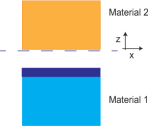
(a)

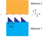
(b)

Figure 1: Schematic of (a) planar structured materials and (b) a planar and an arbitrary periodic shaped structure that will be analyzed in thermal transfer calculations

Green’s function for stratified media:

For the calculation of thermal transfer, we need to calculate the Green function which determines the produced electromagnetic fields in one object (say object 1) that result from current sources in the other object (say object 2). For stratified media composed of a stack of different layers, the contribution of an infinitesimal current $\vec{J}\left(k_{x},k_{y}\right)dz^{\prime}$ to the total electric field produced by it at its own position, denoted by $z^{\prime}$ in object 2, is given by:

$$\overrightarrow{dE_{inc}}\left(z^{\prime}\right)=\frac{-\omega\mu_{0}}{2k_{z}}\left(\hat{p}_{2+}\hat{p}_{2+}+\hat{s}\hat{s}\right)\cdot\vec{J}dz^{\prime}$$ (1)

where $\hat{p}_{2+}$ and $\hat{s}$ refers to the P and S polarization directions for a wave with transverse wave-vector components of $k_{x},k_{y}$. Note that $+$ sign denotes the wave with the wave-vector direction from object 2 toward object 1. From the transfer matrix method, the electric field produced by that element in a location different from its own location, denoted by $z$ in material 1, is given by:

$$\overrightarrow{dE_{inc}}\left(z\right)=\frac{-\omega\mu_{0}}{2k_{z}}\left(t_{21}^{p}\hat{p}_{1+}\hat{p}_{2+}+t_{21}^{s}\hat{s}\hat{s}\right)\cdot\vec{J}dz^{\prime}$$ (2)

where $\hat{p}_{1+}$ refers to P polarization direction in object 1, and $t_{21}^{s}$ and $t_{21}^{p}$ refers to transmission coefficients from $z^{\prime}$ to $z$, for S and P polarizations, respectively.

Accordingly, the dyadic Green function is given through the following expression:

$$\overleftrightarrow{G}\left(z,z^{\prime}\right)=\frac{-\omega\mu_{0}}{2k_{z}}\left(t_{21}^{p}\hat{p}_{1+}\hat{p}_{2+}+t_{21}^{s}\hat{s}\hat{s}\right)$$ (3)

This exactly follows Sipe’s derivation for the Green function.

In the simple case of a slab adjacent to air, this formalism can be simplified further. In this case, we assume the boundary between them is located at $z=0$ and the observation point be located inside air at $z=0$. Moreover, we assume that a current source to be located inside the slab at a distance $z^{\prime}$ from the object’s surface.

Denoting the transversal wave vector by $\beta\hat{\beta}=k_{x}\hat{x}+k_{y}\hat{y}$, the total wave vector in the air and slab can be expressed as:

$$\vec{k_{1}} =\beta\hat{\beta}+k_{zv}\hat{z}$$ (4)

$$\vec{k_{2}} =\beta\hat{\beta}+k_{z}\hat{z}$$ (5)

Also the S and P polarization directions can be expressed as:

$$\hat{p}_{2+} =\frac{c}{\sqrt{\epsilon}\omega}\left(\beta\hat{z}-k_{z}\hat{\beta}\right)$$ (6)

$$\hat{p}_{1+} =\frac{c}{\omega}\left(\beta\hat{z}-k_{zv}\hat{\beta}\right)$$ (7)

$$\hat{s} =\hat{\beta}\times\hat{z}$$ (8)

Moreover in this case, $t_{21}^{p}$ and $t_{21}^{s}$ are simple Fresnel coefficients:

$$t_{21}^{p} =\frac{2\sqrt{\epsilon}k_{z}}{k_{z}+\epsilon k_{zv}}e^{-ik_{z}z^{\prime}}$$ (9)

$$t_{21}^{s} =\frac{2k_{z}}{k_{z}+k_{zv}}e^{-ik_{z}z^{\prime}}$$ (10)

So the dyadic Green function can easily be derived as:

$$\overleftrightarrow{G}= -\frac{\mu_{0}c^{2}e^{-ik_{z}z^{\prime}}}{\omega\left(k_{z}+\epsilon k_{zv}\right)}\left(\beta\hat{z}-k_{zv}\hat{\beta}\right)\left(\beta\hat{z}-k_{z}\hat{\beta}\right)$$

$$-\frac{\mu_{0}\omega e^{-ik_{z}z^{\prime}}}{k_{z}+k_{zv}}\left(\hat{\beta}\times\hat{z}\right)\left(\hat{\beta}\times\hat{z}\right)$$ (11)

with the following components:

$$\overleftrightarrow{G}=\begin{bmatrix}\frac{-k_{x}^{2}}{\omega\epsilon_{0}\beta^{2}}\frac{k_{zv}k_{z}e^{-ik_{z}z^{\prime}}}{k_{z}+\epsilon k_{zv}}-\frac{\omega\mu_{0}}{\beta^{2}}\frac{k_{y}^{2}e^{-ik_{z}z^{\prime}}}{k_{z}+k_{zv}}&\frac{-k_{x}k_{y}}{\omega\epsilon_{0}\beta^{2}}\frac{k_{zv}k_{z}e^{-ik_{z}z^{\prime}}}{k_{z}+\epsilon k_{zv}}+\frac{\omega\mu_{0}}{\beta^{2}}\frac{k_{x}k_{y}e^{-ik_{z}z^{\prime}}}{k_{z}+k_{zv}}&\frac{1}{\omega\epsilon_{0}}\frac{k_{zv}k_{x}e^{-ik_{z}z^{\prime}}}{k_{z}+\epsilon k_{zv}}\\ \frac{-k_{y}k_{x}}{\omega\epsilon_{0}\beta^{2}}\frac{k_{zv}k_{z}e^{-ik_{z}z^{\prime}}}{k_{z}+\epsilon k_{zv}}+\frac{\omega\mu_{0}}{\beta^{2}}\frac{k_{x}k_{y}e^{-ik_{z}z^{\prime}}}{k_{z}+k_{zv}}&\frac{-k_{y}^{2}}{\omega\epsilon_{0}\beta^{2}}\frac{k_{zv}k_{z}e^{-ik_{z}z^{\prime}}}{k_{z}+\epsilon k_{zv}}-\frac{\omega\mu_{0}}{\beta^{2}}\frac{k_{x}^{2}e^{-ik_{z}z^{\prime}}}{k_{z}+k_{zv}}&\frac{1}{\omega\epsilon_{0}}\frac{k_{y}k_{zv}e^{-ik_{z}z^{\prime}}}{k_{z}+\epsilon k_{zv}}\\ \frac{1}{\omega\epsilon_{0}}\frac{k_{x}k_{z}e^{-ik_{z}z^{\prime}}}{k_{z}+\epsilon k_{zv}}&\frac{1}{\omega\epsilon_{0}}\frac{k_{y}k_{z}e^{-ik_{z}z^{\prime}}}{k_{z}+\epsilon k_{zv}}&\frac{-\beta^{2}}{\omega\epsilon_{0}}\frac{e^{-ik_{z}z^{\prime}}}{k_{z}+\epsilon k_{zv}}\end{bmatrix}$$ (12)

These components become the more known results if $k_{y}$ is assumed to be zero, as shown for instance in reference (Polder and Van Hove, 1971):

$$\overleftrightarrow{G} =$$

$$\begin{bmatrix}\frac{-1}{\omega\epsilon_{0}}\frac{k_{zv}k_{z}e^{-ik_{z}z^{\prime}}}{k_{z}+\epsilon k_{zv}}&0&\frac{1}{\omega\epsilon_{0}}\frac{k_{zv}k_{x}e^{-ik_{z}z^{\prime}}}{k_{z}+\epsilon k_{zv}}\\ 0&\frac{-\omega\mu_{0}e^{-ik_{z}z^{\prime}}}{k_{z}+k_{zv}}&0\\ \frac{1}{\omega\epsilon_{0}}\frac{k_{x}k_{z}e^{-ik_{z}z^{\prime}}}{k_{z}+\epsilon k_{zv}}&0&\frac{-1}{\omega\epsilon_{0}}\frac{k_{x}^{2}e^{-ik_{z}z^{\prime}}}{k_{z}+\epsilon k_{zv}}\end{bmatrix}$$ (13)

It is clear that the these results can be easily generalized to more complicated planar structures by deriving more general expressions for the Fresnel coefficients.

Generalization of the Green’s function to periodic structures:

In the general case of periodic structures, we have:

$$\overleftrightarrow{G_{E}}\left(\omega,x,y,z,\beta\hat{\beta},z^{\prime}\right)=$$

$$-\frac{\omega\mu_{0}}{2k_{z}}\overrightarrow{Res_{E}}\left(\omega,x,y,z,\beta\hat{\beta},z^{\prime},\hat{p}_{2+}\right)\hat{p}_{2+}$$

$$-\frac{\omega\mu_{0}}{2k_{z}}\overrightarrow{Res_{E}}\left(\omega,x,y,z,\beta\hat{\beta},z^{\prime},\hat{s}\right)\hat{s}$$ (14)

where $\overrightarrow{Res_{E}}\left(\omega,x,y,z,\beta\hat{\beta},z^{\prime},\hat{p}_{2+}\right)$ and $\overrightarrow{Res_{E}}\left(\omega,x,y,z,\beta\hat{\beta},z^{\prime},\hat{s}\right)$ are electric field responses at position $x,y,z$ to the P and S polarized incident plane wave with transversal wave-vector $\beta\hat{\beta}$ and unity electric field amplitude at position $z^{\prime}$ and angular frequency $\omega$. This is the modified version of sipe’s formalism (Sipe, 1987).

Similarly, for the magnetic field, the following Green function is defined:

$$\overleftrightarrow{G_{H}}\left(\omega,x,y,z,\beta\hat{\beta},z^{\prime}\right)=$$

$$-\frac{\omega\mu_{0}}{2k_{z}}\overrightarrow{Res_{H}}\left(\omega,x,y,z,\beta\hat{\beta},z^{\prime},\hat{p}_{2+}\right)\hat{p}_{2+}$$

$$-\frac{\omega\mu_{0}}{2k_{z}}\overrightarrow{Res_{H}}\left(\omega,x,y,z,\beta\hat{\beta},z^{\prime},\hat{s}\right)\hat{s}$$ (15)

where $\overrightarrow{Res_{H}}\left(\omega,x,y,z,\beta\hat{\beta},z^{\prime},\hat{p}_{2+}\right)$ and $\overrightarrow{Res_{H}}\left(\omega,x,y,z,\beta\hat{\beta},z^{\prime},\hat{s}\right)$ are magnetic field responses at position $x,y,z$ to the P and S polarized incident plane wave, again with transversal wave vector $\beta\hat{\beta}$ and unity electric field amplitude at position $z^{\prime}$ and angular frequency of $\omega$.

From these, in the general case of periodic structures, for the current density of $\vec{J}\left(\omega,k_{x}^{\prime},k_{y}^{\prime},z^{\prime}\right)=\vec{J}\left(\omega,k_{x},k_{y},z_{0}\right)\delta\left(k_{x}^{\prime}-k_{x}\right)\delta\left(k_{y}^{\prime}-k_{y}\right)\delta\left(z^{\prime}-z_{0}\right)$, the generated electric and magnetic field components at position $x,y$ and $z=0$ are given by:

$$\overrightarrow{E_{a}}\left(\omega,x,y,z=0,k_{x},k_{y},z_{0}\right)=\frac{-\omega\mu_{0}}{2k_{z}}e^{-ik_{z}\left(k_{x},k_{y}\right)z_{0}}$$

$$\times\sum_{b}\Big{(}\overrightarrow{Res_{E}}\left(\omega,x,y,\beta\hat{\beta},\hat{p}_{2+}\right)\hat{p}_{2+}$$

$$+\overrightarrow{Res_{E}}\left(\omega,x,y,\beta\hat{\beta},\hat{s}\right)\hat{s}\Big{)}_{ab}\vec{J}_{b}\left(\omega,k_{x},k_{y},z_{0}\right)$$ (16)

$$\overrightarrow{H_{a}}\left(\omega,x,y,z=0,k_{x},k_{y},z_{0}\right)=\frac{-\omega\mu_{0}}{2k_{z}}e^{-ik_{z}\left(k_{x},k_{y}\right)z_{0}}$$

$$\times\sum_{b}\Big{(}\overrightarrow{Res_{H}}\left(\omega,x,y,\beta\hat{\beta},\hat{p}_{2+}\right)\hat{p}_{2+}$$

$$+\overrightarrow{Res_{H}}\left(\omega,x,y,\beta\hat{\beta},\hat{s}\right)\hat{s}\Big{)}_{ab}\vec{J}_{b}\left(\omega,k_{x},k_{y},z_{0}\right)$$ (17)

where

$$\overrightarrow{Res_{E}}\left(\omega,x,y,\beta\hat{\beta},\hat{p}_{2+}\right)\triangleq$$

$$\overrightarrow{Res_{E}}\left(\omega,x,y,z=0,\beta\hat{\beta},z^{\prime}=0,\hat{p}_{2+}\right)$$ (18)

$$\overrightarrow{Res_{H}}\left(\omega,x,y,\beta\hat{\beta},\hat{p}_{2+}\right)\triangleq$$

$$\overrightarrow{Res_{H}}\left(\omega,x,y,z=0,\beta\hat{\beta},z^{\prime}=0,\hat{p}_{2+}\right)$$ (19)

$$\overrightarrow{Res_{E}}\left(\omega,x,y,\beta\hat{\beta},\hat{s}\right)\triangleq$$

$$\overrightarrow{Res_{E}}\left(\omega,x,y,z=0,\beta\hat{\beta},z^{\prime}=0,\hat{s}\right)$$ (20)

$$\overrightarrow{Res_{H}}\left(\omega,x,y,\beta\hat{\beta},\hat{s}\right)\triangleq$$

$$\overrightarrow{Res_{H}}\left(\omega,x,y,z=0,\beta\hat{\beta},z^{\prime}=0,\hat{s}\right)$$ (21)

We assumed the z direction to be normal to plane of top slab. The convention used for the x direction is also shown in Fig. 1. In the above equations, $z=0$ is chosen as the the place of the top slab. In fact we are interested only in the calculation of electromagnetic fields in this location; since by knowing the transverse components of $\vec{E}$ and $\vec{H}$ field in this plane, we can calculate the Poynting vector which determines the heat transfer. This plane is shown with dashed line in Figs. 1a and 1b.

For simplification of the later equations, we define $\overrightarrow{G_{E}^{a}}\left(\omega,x,y,k_{x},k_{y}\right)$ and $\overrightarrow{G_{H}^{a}}\left(\omega,x,y,k_{x},k_{y}\right)$ as the following:

$$\overrightarrow{G_{E}^{a}}\left(\omega,x,y,k_{x},k_{y}\right)\triangleq\frac{-\omega\mu_{0}}{2k_{z}}$$

$$\times\sum_{b}\Big{(}\overrightarrow{Res_{E}}\left(\omega,x,y,\beta\hat{\beta},\hat{p}_{2+}\right)\hat{p}_{2+}$$

$$+\overrightarrow{Res_{E}}\left(\omega,x,y,\beta\hat{\beta},\hat{s}\right)\hat{s}\Big{)}_{ba}\hat{e}_{b}$$ (22)

$$\overrightarrow{G_{H}^{a}}\left(\omega,x,y,k_{x},k_{y}\right)\triangleq\frac{-\omega\mu_{0}}{2k_{z}}$$

$$\times\sum_{b}\Big{(}\overrightarrow{Res_{H}}\left(\omega,x,y,\beta\hat{\beta},\hat{p}_{2+}\right)\hat{p}_{2+}$$

$$+\overrightarrow{Res_{H}}\left(\omega,x,y,\beta\hat{\beta},\hat{s}\right)\hat{s}\Big{)}_{ba}\hat{e}_{b}$$ (23)

where $\hat{e}_{b}$ is the unity vector in direction b, which takes on the unity vectors in x,y, and z directions in the summation. These are the electric and magnetic fields at position $x$, $y$, and $z=0$, produced by the unity component $a$ of the current density at $z^{\prime}=0$. Note that $\overrightarrow{Res_{E}}\left(\omega,x,y,\beta\hat{\beta},\hat{p}_{2+}\right)$, $\overrightarrow{Res_{E}}\left(\omega,x,y,\beta\hat{\beta},\hat{s}\right)$, $\overrightarrow{Res_{H}}\left(\omega,x,y,\beta\hat{\beta},\hat{p}_{2+}\right)$, and $\overrightarrow{Res_{H}}\left(\omega,x,y,\beta\hat{\beta},\hat{s}\right)$ are the electromagnetic responses of the system that can be obtained through the RCWA method. Consequently, $\overrightarrow{G_{E}^{a}}\left(\omega,x,y,k_{x},k_{y}\right)$ and $\overrightarrow{G_{H}^{a}}\left(\omega,x,y,k_{x},k_{y}\right)$ can be calculated directly from the RCWA method, as well.

Therefore, for a general current density distribution $\vec{J}\left(\omega,x_{0},y_{0},z_{0}\right)$ in the top material, we can write $\vec{E}$ and $\vec{H}$ at position $x$, $y=0$, and $z=0$, in the following general form:

$$\overrightarrow{E}\left(x,y=0,z=0,t\right)=\frac{1}{\left(2\pi\right)^{3}}\int_{\omega=0}^{+\infty}d\omega e^{i\omega t}\int\vec{dr_{0}}$$

$$\times\sum_{a}\int_{k_{y}=-\infty}^{+\infty}\int_{k_{x}=-\infty}^{+\infty}dk_{x}dk_{y}e^{-ik_{x}x_{0}-ik_{y}y_{0}-ik_{z}\left(k_{x},k_{y}\right)z_{0}}$$

$$\times\overrightarrow{G_{E}^{a}}\left(\omega,x,y=0,k_{x},k_{y}\right)\vec{J}_{a}\left(\omega,x_{0},y_{0},z_{0}\right)+\text{{c.c.}}$$ (24)

$$\overrightarrow{H}\left(x,y=0,z=0,t\right)=\frac{1}{\left(2\pi\right)^{3}}\int_{\omega=0}^{+\infty}d\omega e^{i\omega t}\int\vec{dr_{0}}$$

$$\times\sum_{b}\int_{k_{y}=-\infty}^{+\infty}\int_{k_{x}=-\infty}^{+\infty}dk_{x}dk_{y}e^{-ik_{x}x_{0}-ik_{y}y_{0}-ik_{z}\left(k_{x},k_{y}\right)z_{0}}$$

$$\times\overrightarrow{G_{H}^{b}}\left(\omega,x,y=0,k_{x},k_{y}\right)\vec{J}_{b}\left(\omega,x_{0},y_{0},z_{0}\right)+\text{{c.c.}}$$ (25)

where $a$, $b$ denotes the three possible components of the current density, and $\overrightarrow{G_{E}^{a}}\left(\omega,x,y=0,k_{x},k_{y}\right)$ and $\overrightarrow{G_{H}^{b}}\left(\omega,x,y=0,k_{x},k_{y}\right)$, are defined in the above. Also c.c. refers to complex conjugate.

According to the above equations, the following expression for the Poynting vector is found:

$$\overrightarrow{P}\left(x,y=0,z=0\right)=\frac{1}{\left(2\pi\right)^{6}}\sum_{a,b}\int_{\omega=0}^{+\infty}\int_{\omega^{\prime}=0}^{+\infty}d\omega^{\prime}d\omega$$

$$\times e^{i\left(\omega-\omega^{\prime}\right)t}\int\int\vec{dr_{0}}\vec{dr_{0}^{\prime}}\left\langle\vec{J}_{a}\left(\omega,\vec{r_{0}}\right)\vec{J}_{b}^{*}\left(\omega^{\prime},\vec{r_{0}^{\prime}}\right)\right\rangle$$

$$\times\int_{k_{y}^{\prime}=-\infty}^{+\infty}\int_{k_{x}^{\prime}=-\infty}^{+\infty}\int_{k_{y}=-\infty}^{+\infty}\int_{k_{x}=-\infty}^{+\infty}dk_{x}dk_{y}dk_{x}^{\prime}dk_{y}^{\prime}$$

$$\times\left(\overrightarrow{G_{E}^{a}}\left(\omega,x,y=0,k_{x},k_{y}\right)\times\overrightarrow{G_{H}^{b*}}\left(\omega^{\prime},x,y=0,k_{x}^{\prime},k_{y}^{\prime}\right)\right)$$

$$\times e^{-ik_{x}x_{0}-ik_{y}y_{0}-ik_{z}z_{0}+ik_{x}^{\prime}x_{0}^{\prime}+ik_{y}^{\prime}y_{0}^{\prime}+ik_{z}^{\prime*}z_{0}^{\prime}}+\text{{c.c.}}$$ (26)

Random thermal motions of charges inside a material, generate fluctuating current densities. These current densities, for a material that is in the thermodynamic equilibrium at temperature T, obey the following correlation relation known as fluctuation dissipation theorem (Eckhardt, 1982; Joulain et al., 2005):

$$\left\langle\vec{J}_{a}\left(\omega,\vec{r_{0}}\right)\vec{J}_{b}^{*}\left(\omega^{\prime},\vec{r_{0}^{\prime}}\right)\right\rangle=4\pi\epsilon_{0}\epsilon^{\prime\prime}\left(\omega\right)\hbar\omega^{2}$$

$$\times\left(e^{\hbar\omega/k_{b}T}-1\right)^{-1}\delta_{ab}\delta\left(\omega-\omega^{\prime}\right)\delta\left(\vec{r_{0}}-\vec{r_{0}^{\prime}}\right)$$ (27)

After making a simplification using the fluctuation dissipation theorem, we have:

$$\overrightarrow{P}\left(x,y=0,z=0\right)=\frac{1}{16\pi^{5}}\sum_{a}\int_{\omega=0}^{+\infty}d\omega\int\vec{dr_{0}}\epsilon_{0}$$

$$\times\epsilon^{\prime\prime}\left(\omega\right)\hbar\omega^{2}\left(e^{\hbar\omega/k_{b}T}-1\right)^{-1}$$

$$\times\int_{k_{y}^{\prime}=-\infty}^{+\infty}\int_{k_{x}^{\prime}=-\infty}^{+\infty}\int_{k_{y}=-\infty}^{+\infty}\int_{k_{x}=-\infty}^{+\infty}dk_{x}dk_{y}dk_{x}^{\prime}dk_{y}^{\prime}$$

$$\times\left(\overrightarrow{G_{E}^{a}}\left(\omega,x,y=0,k_{x},k_{y}\right)\times\overrightarrow{G_{H}^{a*}}\left(\omega,x,y=0,k_{x}^{\prime},k_{y}^{\prime}\right)\right)$$

$$\times e^{i\left(k_{x}^{\prime}-k_{x}\right)x_{0}+i\left(k_{y}^{\prime}-k_{y}\right)y_{0}}e^{i\left(k_{z}^{\prime*}-k_{z}\right)z_{0}}+\text{{c.c.}}$$ (28)

after interchanging the order of integrations, we arrive at:

$$\overrightarrow{P}\left(x,y=0,z=0\right)=\frac{1}{16\pi^{5}}\sum_{a}\int_{\omega=0}^{+\infty}d\omega\epsilon_{0}\epsilon^{\prime\prime}\left(\omega\right)$$

$$\times\int_{k_{y}^{\prime}=-\infty}^{+\infty}\int_{k_{x}^{\prime}=-\infty}^{+\infty}\int_{k_{y}=-\infty}^{+\infty}\int_{k_{x}=-\infty}^{+\infty}dk_{x}dk_{y}dk_{x}^{\prime}dk_{y}^{\prime}$$

$$\times\left(\overrightarrow{G_{E}^{a}}\left(\omega,x,y=0,k_{x},k_{y}\right)\times\overrightarrow{G_{H}^{a*}}\left(\omega,x,y=0,k_{x}^{\prime},k_{y}^{\prime}\right)\right)$$

$$\times\hbar\omega^{2}\int_{z_{0}=0}^{\infty}\int_{y_{0}=-\infty}^{\infty}\int_{x_{0}=-\infty}^{\infty}dx_{0}dy_{0}dz_{0}e^{i\left(k_{z}^{\prime*}-k_{z}\right)z_{0}}$$

$$\times e^{i\left(k_{x}^{\prime}-k_{x}\right)x_{0}+i\left(k_{y}^{\prime}-k_{y}\right)y_{0}}\left(e^{\hbar\omega/k_{b}T}-1\right)^{-1}+\text{{c.c.}}$$ (29)

which reduces to:

$$\overrightarrow{P}\left(x,y=0,z=0\right)=\frac{1}{4\pi^{3}}\sum_{a}\int_{\omega=0}^{+\infty}d\omega\epsilon_{0}\epsilon^{\prime\prime}\left(\omega\right)$$

$$\times\int_{k_{y}^{\prime}=-\infty}^{+\infty}\int_{k_{x}^{\prime}=-\infty}^{+\infty}\int_{k_{y}=-\infty}^{+\infty}\int_{k_{x}=-\infty}^{+\infty}dk_{x}dk_{y}dk_{x}^{\prime}dk_{y}^{\prime}$$

$$\times\left(\overrightarrow{G_{E}^{a}}\left(\omega,x,y=0,k_{x},k_{y}\right)\times\overrightarrow{G_{H}^{a*}}\left(\omega,x,y=0,k_{x},k_{y}\right)\right)$$

$$\times\hbar\omega^{2}\left(e^{\hbar\omega/k_{b}T}-1\right)^{-1}\delta\left(k_{x}-k_{x}^{\prime}\right)\delta\left(k_{y}-k_{y}^{\prime}\right)$$

$$\times\int_{z_{0}=0}^{\infty}e^{i\left(k_{z}^{\prime*}-k_{z}\right)z_{0}}dz_{0}+\text{{c.c.}}$$ (30)

Finally we obtain that:

$$\overrightarrow{P}\left(z=0,y=0,x\right)=\frac{1}{4\pi^{3}}\sum_{a}\int_{\omega=0}^{+\infty}d\omega\epsilon_{0}\epsilon^{\prime\prime}\left(\omega\right)\hbar\omega^{2}$$

$$\times\left(e^{\hbar\omega/k_{b}T}-1\right)^{-1}\int_{k_{y}=-\infty}^{+\infty}\int_{k_{x}=-\infty}^{+\infty}dk_{x}dk_{y}$$

$$\times\frac{1}{Im\left(k_{z}\right)}\Re\Big{\{}\Big{(}\overrightarrow{G_{E}^{a}}\left(\omega,x,y=0,k_{x},k_{y}\right)$$

$$\times\overrightarrow{G_{H}^{a*}}\left(\omega,x,y=0,k_{x},k_{y}\right)\Big{)}\Big{\}}$$ (31)

Note that the z component of this quantity measures the thermal transfer. The thermal capacitance can be obtained from it through differentiating with respect to temperature:

$$S_{total}(x)=\frac{1}{4\pi^{3}}\sum_{a}\int_{\omega=0}^{+\infty}d\omega\epsilon_{0}\epsilon^{\prime\prime}\left(\omega\right)\left(e^{\hbar\omega/k_{b}T}-1\right)^{-2}$$

$$\times\int_{k_{y}=-\infty}^{+\infty}\int_{k_{x}=-\infty}^{+\infty}dk_{x}dk_{y}\frac{e^{\hbar\omega/k_{b}T}}{Im\left(k_{z}\right)}\frac{\hbar^{2}\omega^{3}}{k_{b}T^{2}}$$

$$\times\Re\Big{\{}\Big{(}\overrightarrow{G_{E}^{a}}\left(\omega,x,y=0,k_{x},k_{y}\right)$$

$$\times\overrightarrow{G_{H}^{a*}}\left(\omega,x,y=0,k_{x},k_{y}\right)\Big{)}_{z}\Big{\}}$$ (32)

In fact, what is measured as the total heat transfer and the corresponding heat capacitance is the average of the above functions across a period, which we show here with the same symbol:

$$S_{total}=\frac{1}{Per}\int_{x=0}^{Per}S_{total}\left(x\right)dx$$ (33)

It is important to note that considering only the fields in a line in x direction saves significant computational time. In fact this is achieved by exploiting the translational symmetry of our structure in y-direction and also the fact that for obtaining the energy flow, it is sufficient to calculate the Poynting vector in a cross section. Note that in our method, the variation of thermal transfer across a cross section can also be obtained. This provides the ability to determine the contributions of different locations across the period to the total thermal transfer or capacitance.

Moreover, in the above calculations, we are involved with only transverse components of the electromagnetic fields. Since these quantities are continuous across the barrier, we need only to calculate the electromagnetic fields in the top material right at the boundary. These fields can be calculated from the reflection coefficients in the RCWA formalism, and will further simply the required RCWA calculations. In fact calculation of the electromagnetic fields in the middle layers and bottom material (transmission coefficients) are not needed anymore. [See section 7 of reference (Moharam et al., 1995b)]

Numerical Results:

In the following, we analyze two different periodic structures with our developed formalism. The first example structure is shown in Fig. 2. In this example, we modified the previously-studied case of two closely-spaced SiC slabs separated from each other by an air gap to a case where one of slabs is patterned with a periodic grating. We expect that the corrugations modify the dispersion relation of the surface phonon polaritons supported by a smooth SiC surface and thereby impact the thermal capacitance . The second structure that we considered, is an array of SiC beams of rectangular cross section placed above a continuous slab of SiC (Fig. 7).

Calculations for the first structure have been done for three different separations between the two SiC structures (specifically $d=1um$, $d=10um$, and $d=0.1um$) and different periodicities (specifically $Per=1um$, $Per=10um$, and $Per=0.1um$). The depth of the grooves in the considered structures is $d_{slit}=0.5d$.

The optical properties of the SiC material is computed based on references (Spitzer et al., 1959a, b) which assumes the following expression for the SiC refractive index and extinction coefficient:

$$n^{2} =\frac{1}{2}\left\{\left[\epsilon^{2}+4\left(\frac{\sigma}{\nu}\right)^{2}\right]^{\frac{1}{2}}+\epsilon\right\}$$ (34)

$$k^{2} =\frac{1}{2}\left\{\left[\epsilon^{2}+4\left(\frac{\sigma}{\nu}\right)^{2}\right]^{\frac{1}{2}}-\epsilon\right\}$$ (35)

where the variables introduced in it are defined as:

$$\epsilon =\epsilon_{0}+4\pi\chi$$ (36)

$$\chi =\rho\frac{1-\nu^{2}/\nu_{0}^{2}}{\left(1-\nu^{2}/\nu_{0}^{2}\right)^{2}+\gamma^{2}\nu^{2}/\nu_{0}^{2}}$$ (37)

$$\frac{\sigma}{\nu} =2\pi\rho\frac{\gamma\nu}{\left(1-\nu^{2}/\nu_{0}^{2}\right)^{2}+\gamma^{2}\nu^{2}/\nu_{0}^{2}}$$ (38)

Containing the following numerical parameters:

$$\rho=0.263,$$

$$\gamma=0.006,$$

$$\nu=2.38\times 10^{13}sec^{-1}(12.6\mu m),\,and$$

$$\epsilon_{0}=6.7$$ (39)

In addition, the temperature that is assumed in the numerical calculations is $T=315K$.

For calculations based on the RCWA method, it is well-known that increasing the number of harmonics leads to a more accurate determination of the field distributions. However, this increase will lead to an increase in computational time as well. In fact since the numerical evaluation of the thermal capacitance by the presented method involves inverting $4n\times 4n$ matrices, the computational time grows with the cube of the number of harmonics incorporated. It is clear from the last equation in theory section that obtaining the spectral thermal capacitance at a specific frequency requires two dimensional integrations in the $k_{x}$,$k_{y}$ plane. For each value of $k_{x}$,$k_{y}$, a RCWA calculation should be carried out to obtain the corresponding integrand. This clarifies the importance of identifying a fast integration technique to maximize the speed of calculations. We have used the VEGAS method for integration in $k_{x}$,$k_{y}$ plane which is based on Monte Carlo important sampling of the integrand function (Peter Lepage, 1978). To verify our calculation technique, we first accurately reproduced the results for the limiting cases of gratings with duty cycles of 0 and 1. In those cases, using just one harmonic will lead to the precise result and the RCWA method will converge to the results that can be obtained with the transfer matrix method for a stratified medium consisting of uniform layers. In these extremum cases we can simply use the planar methods developed by Polder and Van hove (Polder and Van Hove, 1971).

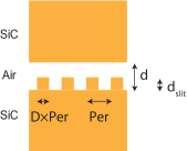
Figure 2: Two SiC slab are placed in front of each other, one with a flat and one with a binary grating structure. The duty cycle of the grating is assumed to be $D$, and its periodicity is shown with $Per$. The distances involved for this structure are shown in the figure.

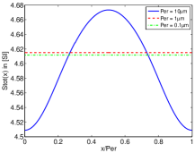
(a)

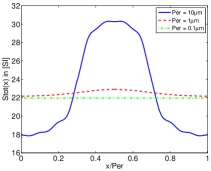
(b)

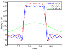
(c)

Figure 3: Contributions to the thermal capacitance for the structure shown in Fig. 2 across a period for different values of periodicity, and assuming a constant duty cycle of $D=0.4$, in the case of (a) $d=10\mu m$ (b) $d=1\mu m$ (c) $d=0.1\mu m$

To study the convergence of the results with the number of harmonics, calculations were made with 4 different numbers of harmonics: 1, 5, 11, and 21. Obtained results show that for the considered structures, the thermal capacitance converges with less than 2% error without the need for incorporating more harmonics. One important note regarding our method is that this method in the case of incorporating just one harmonic, $n=1$, reproduces the results obtained by using the effective medium theory. Note that in the case of using just one harmonic, permittivity of each layer is replaced by a constant value across the period. This constant value, however, takes on different magnitudes depending on the incident electric field direction. This is the case also in the effective medium theories (Biehs et al., 2011a; Basu and Wang, 2013; Biehs et al., 2012, 2013, 2011b), used for calculation of the thermal transfer, in which effective permittivities of different layers are calculated as constant tensorial quantities. In this regard, our method can be used to determine the accuracy of the effective medium theory and how the actual responses are deviating from it.

For this study, these numerical calculations were run on a node with 16 CPU s, using MPI (Gropp et al., 1999) for parallelization (The node that we used for our calculations has 16 processors of 2.67 GHz Intel Xeon X5550). The time required for obtaining each set of results on a single node for the case of 21 harmonics was around 10 hours. However, this can be decreased by capitalizing on certain symmetries in specific periodic structures, which has been proposed for the 2D grating in reference (Bai and Li, 2005) and can be incorporated in 1D grating structures as well (using for instance the inversion symmetry present in the binary grating).

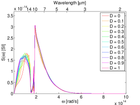
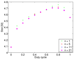
(a)

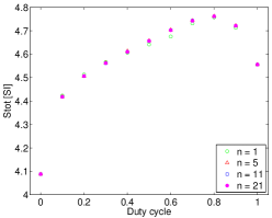
(b)

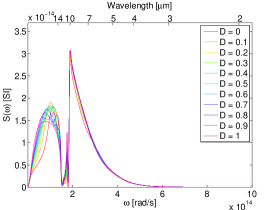
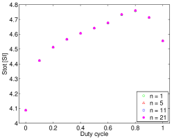
(c)

Figure 4: Spectral contributions to the thermal capacitance and total thermal capacitance for the structure shown in Fig. 2 with d = 10$\mu$m and different values of duty cycle with the periodicity of (a) Per = 10$\mu$m (b) Per = 1$\mu$m (c) Per = 0.1$\mu$m

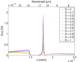
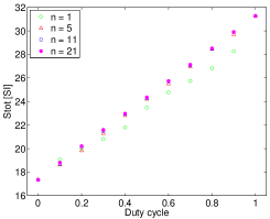
(a)

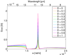
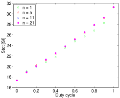
(b)

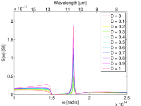
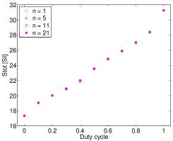
(c)

Figure 5: Spectral contributions to the thermal capacitance and total thermal capacitance for the structure shown in Fig. 2 with d = 1$\mu$m and different values of duty cycle with the periodicity of (a) Per = 10$\mu$m (b) Per = 1$\mu$m (c) Per = 0.1$\mu$m

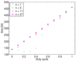
(a)

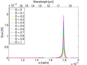
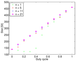
(b)

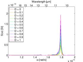
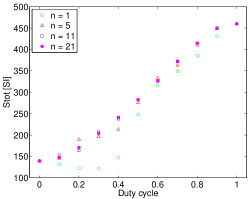
(c)

Figure 6: Spectral contributions to the thermal capacitance and total thermal capacitance for the structure shown in Fig. 2 with d = 0.1$\mu$m and different values of duty cycle with the periodicity of (a) Per = 10$\mu$m (b) Per = 1$\mu$m (c) Per = 0.1$\mu$m

The results of calculation for the structure shown in Fig. 2 at different values of periodicities and distances are summarized in Figs. 4, 5, and 6 respectively for $d=10\mu m$, $d=1\mu m$, and $d=0.1\mu m$. As the figures show, convergence is achieved with incorporation of 21 harmonics in all cases. The total thermal capacitance in most cases is monotonically increasing with increasing duty cycle. This comes from the fact that gratings with higher duty cycles feature more SiC material that is located near the adjacent SiC slab. This then naturally facilitates higher evanescent coupling. However, for the case of $d=10\mu m$, a peak in thermal transfer is achieved for a value of duty cycle which is neither 0 or 1. Noting the fact that the resonance wavelength of the SiC is around $10\mu m$, we expect Mie resonances of the beam to become important in that case and give rise to the highest thermal capacitance for the non-unity duty cycle.

One important fact that can be derived from the obtained results is that, as the periodicity decreases, the result obtained with using just one harmonic becomes more accurate. This is to be expected since in the case of incorporating just one harmonic, our method reproduces results obtained by the effective medium theory which becomes more and more accurate in subwavelength regime (compared with the resonance wavelength).

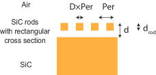
Figure 7: SiC beams with a rectangular cross section are placed in front of a SiC slab. The width of each beam is assumed to be $D\times Per$, and they are separated by a distance $Per$ from each other. The distances involved for this structure are shown in the figure.

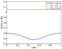
(a)

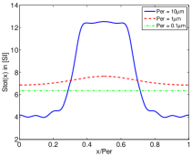
(b)

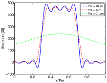
(c)

Figure 8: Contributions to the thermal capacitance for the structure shown in Fig. 7 across a period for different values of periodicity, and assuming a constant value of $D=0.4$, in the case of (a) $d=10\mu m$ (b) $d=1\mu m$ (c) $d=0.1\mu m$

This fact is most evident in Fig. 3, which shows the contribution of different points across the period to the total thermal capacitance. In this figure the thermal capacitance is plotted as a function of $x$ position across the period at $z=0$ plane for different values of periodicity and distances. The duty cycle is assumed to be the same value of $0.4$ in all cases. Note that since we have translational symmetry in the y direction, there is no change in thermal capacitance in that direction. This figure verifies the fact that thermal capacitance in the limit of small periods, tends toward a constant value across the period which is determined by effective medium theory. On the other hand, this figure further demonstrates the fact that for periodicities larger than some critical value, thermal capacitance can be modeled as a superposition of two channels; a channel with larger thermal capacitance which is due to parts of slabs that are closer together and the other one with smaller thermal capacitance which is due to the sections that are farther from each other. These plots were obtained by incorporation of 21 harmonics.

In the second structure we have considered, the thermal capacitance of the SiC beams, and a slab of SiC is numerically calculated. The details of the notations used for the parameters involved in this structure are shown in Fig. 7. Results of the thermal capacitance corresponding to $d=10\mu m$, $d=1\mu m$, and $d=0.1\mu m$ are shown in Figs 9, 10, and 11, respectively. In the structures considered, $d_{rod}=0.5d$, is assumed. Like the previous structure, the thermal capacitance across a period is plotted for different distances and periodicities, using D = 0.4 in all cases. The plots which are shown in Fig. 8 were all obtained by using 21 harmonics.

One important fact regarding this structure is that we should obtain the thermal emission from a slab of SiC to the vacuum for the case of a duty cycle of 0. (In this case there are no beams anymore) Our formalism nicely reproduces this result in this case. Again like for the previous structure we see the monotonically increase in thermal capacitance for the distances of $d=1\mu m$, and $d=0.1\mu m$. Note that this increase is not necessarily linear with the duty cycle. However this increase becomes more linear for large values of periodicity. This again is consistent with our intuition that for large values of periodicity, the cross talk between neighboring beams are negligible.

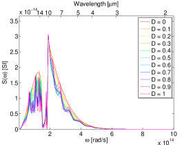
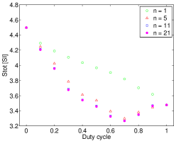
(a)

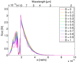
(b)

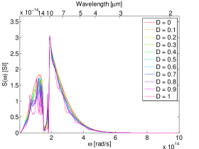
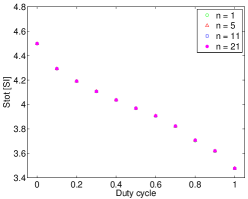
(c)

Figure 9: Spectral contributions to the thermal capacitance and total thermal capacitance for the structure shown in Fig. 7 with d = 10$\mu$m and different values of duty cycle with the periodicity of (a) Per = 10$\mu$m (b) Per = 1$\mu$m (c) Per = 0.1$\mu$m

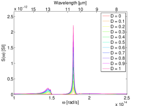
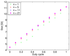
(a)

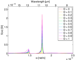
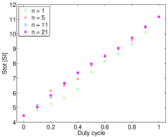
(b)

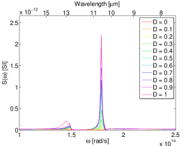
(c)

Figure 10: Spectral contributions to the thermal capacitance and total thermal capacitance for the structure shown in Fig. 7 with d = 1$\mu$m and different values of duty cycle with the periodicity of (a) Per = 10$\mu$m (b) Per = 1$\mu$m (c) Per = 0.1$\mu$m

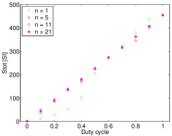
(a)

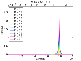
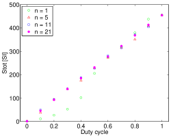
(b)

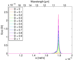
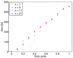
(c)

Figure 11: Spectral contributions to the thermal capacitance and total thermal capacitance for the structure shown in Fig. 7 with d = 0.1$\mu$m and different values of duty cycle with the periodicity of (a) Per = 10$\mu$m (b) Per = 1$\mu$m (c) Per = 0.1$\mu$m

The situation for $d=10\mu m$ with $Per=10\mu m$ is more interesting. In this case as we encountered previously for the grating structure, the extremum of thermal capacitance is achieved for a duty cycle which is neither zero or unity. Here, we again expect the Mie resonances of the nanobeams come into play. Note that in this case, the result of effective medium theory, has the largest inaccuracy. This is expected since in this case the periodicity is the largest compared with the two other cases for $d=10\mu m$. (Specifically, cases of $Per=1\mu m$ and $Per=0.1\mu m$)

One important fact about our method is that it can be used in this way for calculation of thermal transfer between a slab and a particle with an arbitrary shaped structure. This comes from the fact that when the periodicity becomes large, the cross talk between particles becomes negligible and the thermal capacitance is coming from the sum of the contributions of individual beams. This can be proposed as an alternative method for calculation of thermal capacitance between e.g. a sphere and a slab that has been done in several methods in several references (Krüger et al., 2011; Otey and Fan, 2011; McCauley et al., 2012).

Conclusions:

In this paper, we have developed a formalism for calculating the thermal transfer of periodic structures with building blocks of arbitrary size and shape. We applied this method to obtain the thermal capacitance between a slab of SiC and binary SiC gratings. We also used this method for the calculation of the thermal transfer between a plain slab of SiC and an array of SiC beams of rectangular cross section. The obtained results show that, thermal capacitance in these cases can accurately be obtained through incorporation of some of the first harmonics. Moreover, results show that the thermal transfer changes monotonically with increasing duty cycle for the cases that distances are much smaller than the resonance wavelength. However, this trend breaks in the case that distances are on the same order of magnitude as the resonance wavelength.

Our method, in the case of incorporating just one harmonic reproduces the results obtained by the effective medium theory. In this regard, this method can be used to determine the accuracy of the effective medium theory for specific structures of interest. According to the numerical results obtained, as we expect, by decreasing the periodicity of the structure to the subwavelength regime compared with the relevant resonance wavelengths in the system, effective medium theory becomes increasingly accurate.

This method can also be used to analyze the thermal transfer between structures in which one of the materials is composed of an array of particles. Since in the limit of large periodicity, the cross talk between particles becomes negligible, this method poses itself to be used for calculation of thermal transfer between a slab and arbitrary shaped particles. For the reasons above, we believe that the presented technique will prove versatile for calculating and optimizing the thermal transfer between a wide variety of practical structures.

References

- Basu et al. (2007) S. Basu, Y.-B. Chen, and Z. M. Zhang, International Journal of Energy Research 31, 689 (2007).
- Lin et al. (2003) S. Y. Lin, J. Moreno, and J. G. Fleming, Applied Physics Letters 83, 380 (2003).
- De Wilde et al. (2006) Y. De Wilde, F. Formanek, R. Carminati, B. Gralak, P.-A. Lemoine, K. Joulain, J.-P. Mulet, Y. Chen, and J.-J. Greffet, Nature 444, 740 (2006).
- Schuller et al. (2009) J. A. Schuller, T. Taubner, and M. L. Brongersma, Nature Photonics 3, 658 (2009).
- Dahan et al. (2007) N. Dahan, A. Niv, G. Biener, Y. Gorodetski, V. Kleiner, and E. Hasman, Physical Review B 76, 45427 (2007).
- Shitrit et al. (2013) N. Shitrit, I. Yulevich, E. Maguid, D. Ozeri, D. Veksler, V. Kleiner, and E. Hasman, Science (New York, N.Y.) 340, 724 (2013).
- Dahan et al. (2010) N. Dahan, Y. Gorodetski, K. Frischwasser, V. Kleiner, and E. Hasman, Physical Review Letters 105, 136402 (2010).
- Planck (1914) M. Planck, Blakiston’s Son & Co (1914).
- Polder and Van Hove (1971) D. Polder and M. Van Hove, Physical Review B 4, 3303 (1971).
- Shchegrov et al. (2000) A. Shchegrov, K. Joulain, R. Carminati, and J.-J. Greffet, Physical Review Letters 85, 1548 (2000).
- Krüger et al. (2012) M. Krüger, G. Bimonte, T. Emig, and M. Kardar, Physical Review B 86, 115423 (2012).
- Krüger et al. (2011) M. Krüger, T. Emig, and M. Kardar, Physical Review Letters 106, 210404 (2011).
- Otey and Fan (2011) C. Otey and S. Fan, Physical Review B 84, 245431 (2011).
- McCauley et al. (2012) A. P. McCauley, M. T. H. Reid, M. Krüger, and S. G. Johnson, Physical Review B 85, 165104 (2012).
- Reid et al. (2013) M. T. H. Reid, A. W. Rodriguez, and S. G. Johnson, Proceedings of the IEEE 101, 531 (2013).
- Biehs et al. (2011a) S.-A. Biehs, F. S. S. Rosa, and P. Ben-Abdallah, Applied Physics Letters 98, 243102 (2011a).
- Basu and Wang (2013) S. Basu and L. Wang, Applied Physics Letters 102, 53101 (2013).
- Biehs et al. (2012) S.-A. Biehs, M. Tschikin, and P. Ben-Abdallah, Physical Review Letters 109, 104301 (2012).
- Biehs et al. (2013) S.-A. Biehs, M. Tschikin, R. Messina, and P. Ben-Abdallah, Applied Physics Letters 102, 131106 (2013).
- Biehs et al. (2011b) S.-A. Biehs, P. Ben-Abdallah, F. S. S. Rosa, K. Joulain, and J.-J. Greffet, Optics express 19 Suppl 5, A1088 (2011b).
- Wang et al. (2014) L. Wang, A. Haider, and Z. Zhang, Journal of Quantitative Spectroscopy and Radiative Transfer 132, 52 (2014).
- Han (2009) S. Han, Physical Review B 80, 155108 (2009).
- Rodriguez et al. (2011) A. W. Rodriguez, O. Ilic, P. Bermel, I. Celanovic, J. D. Joannopoulos, M. Soljačić, and S. G. Johnson, Physical Review Letters 107, 114302 (2011).
- Bimonte (2009) G. Bimonte, Physical Review A 80, 042102 (2009).
- Moharam et al. (1995a) M. G. Moharam, E. B. Grann, D. A. Pommet, and T. K. Gaylord, Journal of the Optical Society of America A 12, 1068 (1995a).
- Moharam et al. (1995b) M. G. Moharam, D. A. Pommet, E. B. Grann, and T. K. Gaylord, Journal of the Optical Society of America A 12, 1077 (1995b).
- Sipe (1987) J. E. Sipe, Journal of the Optical Society of America B 4, 481 (1987).
- Eckhardt (1982) W. Eckhardt, Optics Communications 41, 305 (1982).
- Joulain et al. (2005) K. Joulain, J.-P. Mulet, F. Marquier, R. Carminati, and J.-J. Greffet, Surface Science Reports 57, 59 (2005).
- Spitzer et al. (1959a) W. Spitzer, D. Kleinman, and D. Walsh, Physical Review 113, 127 (1959a).
- Spitzer et al. (1959b) W. Spitzer, D. Kleinman, and C. Frosch, Physical Review 113, 133 (1959b).
- Peter Lepage (1978) G. Peter Lepage, Journal of Computational Physics 27, 192 (1978).
- Gropp et al. (1999) W. Gropp, E. Lusk, and A. Skjellum, Using MPI: Portable parallel programming with the message-passing interface (MIT Press (Cambridge, Mass.), 1999).
- Bai and Li (2005) B. Bai and L. Li, Journal of Optics A: Pure and Applied Optics 7, 783 (2005).