Measuring the X-ray luminosities of SDSS DR7 clusters from RASS

Abstract

We use ROSAT All Sky Survey (RASS) broadband X-ray images and the optical clusters identified from SDSS DR7 to estimate the X-ray luminosities around $\sim 65,000$ candidate clusters with masses $\ga 10^{13}\>h^{-1}\rm M_{\odot}$ based on an Optical to X-ray (OTX) code we develop. We obtain a catalogue with X-ray luminosity for each cluster. This catalog contains 817 clusters (473 at redshift $z\leq 0.12$) with $S/N>3$ in X-ray detection. We find about $65\%$ of these X-ray clusters have their most massive member located near the X-ray flux peak; for the rest $35\%$, the most massive galaxy is separated from the X-ray peak, with the separation following a distribution expected from a NFW profile. We investigate a number of correlations between the optical and X-ray properties of these X-ray clusters, and find that: the cluster X-ray luminosity is correlated with the stellar mass (luminosity) of the clusters, as well as with the stellar mass (luminosity) of the central galaxy and the mass of the halo, but the scatter in these correlations is large. Comparing the properties of X-ray clusters of similar halo masses but having different X-ray luminosities, we find that massive halos with masses $\ga 10^{14}\>h^{-1}\rm M_{\odot}$ contain a larger fraction of red satellite galaxies when they are brighter in X-ray. An opposite trend is found in central galaxies in relative low-mass halos with masses $\la 10^{14}\>h^{-1}\rm M_{\odot}$ where X-ray brighter clusters have smaller fraction of red central galaxies. Clusters with masses $\ga 10^{14}\>h^{-1}\rm M_{\odot}$ that are strong X-ray emitters contain many more low-mass satellite galaxies than weak X-ray emitters. These results are also confirmed by checking X-ray clusters of similar X-ray luminosities but having different characteristic stellar masses. A cluster catalog containing the optical properties of member galaxies and the X-ray luminosity is available at http://gax.shao.ac.cn/data/Group.html.

1 Introduction

Clusters of galaxies are the most massive virialized objects in the universe. Their abundance and spatial distribution are powerful cosmological probes (e.g., Majumdar & Mohr 2004; Vikhlinin et al. 2009b; Mantz et al. 2010a). In addition, galaxy clusters provide extreme environments for studying the formation and evolution of galaxies within the framework of the hierarchical build-up of the most massive halos. One important property of clusters is that both their stellar and gas components are readily observable: their gravitational wells are deep enough to retain energetic gas ejected from their member galaxies which can be observed in optical and infrared. The intracluster medium (ICM) is also hot enough to be observable in X-ray. The observed thermodynamic state of the ICM is determined by the combined effects of shock heating during accretion, radiative cooling, feedback from stellar evolution (stellar winds and supernovae) and active galactic nuclei, as well as the magnetic fields, cosmic rays and turbulence. The density, temperature, and entropy profiles of the ICM therefore carry important information regarding the entire thermal history of cluster formation. The hot ICM, with temperatures between $10^{7}$K and $10^{8}$K, emits X-rays in the form of thermal bremsstrahlung and atomic line emissions (e.g., Kellogg et al. 1971; Forman et al. 1971). By assuming hydrostatic equilibrium between the intracluster gas and the cluster potential, one can also derive the gravitational mass of the cluster using density and temperature measurements provided by X-ray data.

Clusters have also been observed by other means in addition to X-ray: optical, infrared, radio, Sunyaev-Zel’dovich effect and gravitational lensing. Among these, the most complete cluster samples to date are optically-selected either from photometric or spectroscopic data. Photometrically selected complete cluster samples can be constructed for the most massive clusters and in large redshift ranges. However, the properties of their galaxy members are not well understood. In order to have reliable membership assignments of galaxies to dark matter halos, which is important for understanding galaxy formation and evolution in such systems, spectroscopic data are needed. During the past two decades, numerous group catalogues have been constructed from various redshift surveys of galaxies, most noticeably the CfA redshift survey (e.g. Geller & Huchra 1983), the Las Campanas Redshift Survey (e.g. Tucker et al. 2000), the 2-degree Field Galaxy Redshift Survey (hereafter 2dFGRS; Merchán & Zandivarez 2002; Eke et al. 2004, Yang et al. 2005; Tago et al. 2006; Einasto et al. 2007), the high-redshift DEEP2 survey (Gerke et al. 2005), and the Two Micron All Sky Redshift Survey (Crook et al. 2007). Various group catalogues have also been constructed from redshift samples selected from the Sloan Digital Sky Survey (hereafter SDSS) using different methods: friends-of-friends (FOF) algorithm (e.g. Goto 2005; Merchán & Zandivarez 2005; Berlind et al. 2006), the C4 algorithm (Miller et al. 2005), and the halo-based group finder (e.g., Yang et al. 2005; Weinmann et al. 2006; Yang et al. 2007). These catalogs provide galaxy groups that have reliable galaxy memberships, which is important in probing the halo occupation distribution (HOD) statistics and galaxy formation models (e.g. Yang et al. 2008; 2009).

X-ray selection of galaxy clusters is reliable but typically has a low efficiency. Indeed, even if survey selections are properly taken into account, a significant fraction of optically detected clusters that obey the scaling relation between optical luminosity and virial mass (inferred from, e.g., the velocity dispersion of member galaxies) are undetected in X-ray (i.e., they do not follow the scaling relation between X-ray luminosity and virial mass). This has given rise to the notion that there exists a genuine population of clusters that are X-ray under-luminous (e.g., Castander et al. 1994; Lubin et al. 2004; Popesso et al. 2007; Castellano et al. 2011; Balogh et al. 2011). However, as will be illustrated later, such an incompleteness in X-ray cluster detection is mainly due to the blind search of X-ray peaks in relatively shallow observations. If prior information about the positions and sizes of the candidate X-ray clusters is available, the X-ray detection completeness can be improved dramatically. In this paper, we study the X-ray properties of the optical clusters selected by Yang et al. (2007) from the SDSS DR7 using the algorithm developed in Shen et al. (2008), which enables us to obtain a much more complete X-ray cluster catalog than currently available. The X-ray information so obtained adds to the wealth of optical information in the SDSS DR7 group catalog, together providing a useful data base to study galaxy formation and evolution in clusters of galaxies.

This paper is organized as follows. In Section 2, we briefly describe the group samples to be used. In Section 3, we outline our Optical to X-ray (OTX) code used to estimate the X-ray luminosities around optical clusters and test the reliability of our X-ray luminosity measurement using existing known X-ray clusters. Basic X-ray properties of these clusters are investigated in Section 4. Finally, we present our conclusions in Section 5.

Throughout this paper, we use the $\Lambda$CDM cosmology whose parameters are consistent with the 7-year data release of the WMAP mission: $\Omega_{\rm m}=0.275$, $\Omega_{\rm\Lambda}=0.725$, $h=0.702$, and $\sigma_{8}=0.816$, where the reduced Hubble constant, $h$, is defined through the Hubble constant as $H_{0}=100h~{}{\rm km~{}s^{-1}~{}Mpc^{-1}}$ (Komatsu et al. 2011). If not specified otherwise, we use $L_{\rm X}$, $F_{\rm X}$, $T_{\rm X}$, $M_{h}$, $r_{200}$, to denote the X-ray luminosity, flux, gas temperature, halo mass and halo radius of each X-ray cluster. These quantities are quoted in units of $10^{44}{\rm erg~{}s^{-1}}$, $10^{-12}{\rm erg~{}s^{-1}~{}cm^{-2}}$, ${\rm keV}$, $\>h^{-1}\rm M_{\odot}$ and $\>h^{-1}{\rm{Mpc}}$, respectively.

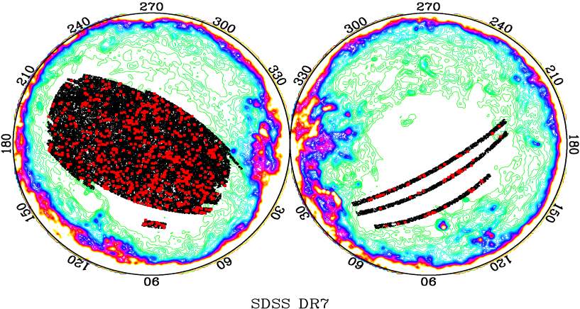
Figure 1: The sky coverage of the SDSS DR7 clusters with mass $\ga 10^{13}\>h^{-1}\rm M_{\odot}$ (black area), overlaid on the galactic extinction contours of Schlegel, Finkbeiner & Davis (1998). The red squares show the distribution of X-ray clusters with $S/N>3$ detections.

2 The SDSS DR7 Galaxy and Group catalogs

The optical data used in our analysis is taken from the SDSS galaxy group catalogs of Yang et al. (2007; hereafter Y07), constructed using the adaptive halo-based group finder of Yang et al. (2005), here updated to Data Release 7 (DR7). The parent galaxy catalog is the New York University Value-Added Galaxy catalog (NYU-VAGC; Blanton et al. 2005) based on the SDSS DR7 (Abazajian et al. 2009), which contains an independent set of significantly improved reductions. DR7 marks the completion of the survey phase known as SDSS-II. It features a spectroscopic sample that is now complete over a large contiguous area of the Northern Galactic cap, closing the gap which was present in previous data releases. From the NYU-VAGC, we select all galaxies in the Main Galaxy Sample with an extinction-corrected apparent magnitude brighter than $r=17.72$, with redshifts in the range $0.01\leq z\leq 0.20$ and with a redshift completeness ${\cal C}_{z}>0.7$. The resulting SDSS galaxy catalog contains a total of $639,359$ galaxies, with a sky coverage of 7748 square degrees. Note that a very small fraction of galaxies in this catalog have redshifts taken from the Korea Institute for Advanced Study (KIAS) Value-Added Galaxy Catalog (VAGC) (e.g. Choi et al. 2010). There are $36,759$ galaxies that do not have redshift measurements due to fiber collisions, but are assigned the redshifts of their nearest neighbors.

In this study, in order not to miss any potential group members for cross-identification, we use the group catalog which is constructed for all the galaxies, where model magnitudes are used for the group finding. In total, there are $472,416$ groups in our catalog within which about $23,700$ have three member galaxies or more. Following Y07, for each group in the catalog, we estimate the corresponding halo mass using the ranking of its characteristic stellar mass, defined as the total stellar mass of all group members with $\>{}^{0.1}{\rm M}_{r}-5\log h\leq-19.5$. Here the halo mass function obtained by Tinker et al. (2008) for WMAP7 cosmology and $\Delta=200$ is used in our calculation, where $\Delta$ is the average mass density contrast in the spherical halo. We indicate the group mass obtained this way by $M_{\rm h}$ or $M_{200}$. Note that groups whose member galaxies are all fainter than $\>{}^{0.1}{\rm M}_{r}-5\log h=-19.5$ cannot be assigned a halo mass with this method. For these systems, one could in principle use the relation between halo mass and the stellar mass of the central galaxy obtained by Yang et al. (2012) to estimate their halo masses. However, since our main focus is on probing the X-ray and optical properties of massive clusters, we do not need halo masses for these low mass groups.

According to our definition of halo mass $M_{\rm h}$ ($M_{200}$), a halo has an average overdensity of 200 times the mean density of the universe within its ‘virial radius’, $r_{200}$, which is given by

$$r_{\rm 200}=\left[\frac{M_{200}}{\frac{4\pi}{3}\times 200\Omega_{\rm m}\times\frac{3H_{0}^{2}}{8\pi G}}\right]^{1/3}(1+z)^{-1}\,,$$ (1)

where $z$ is the redshift of the group (i.e., the average redshift of its members). Tests with detailed mock galaxy redshift surveys, which take into account various survey selection effects, uncertainties in the group finder and halo mass estimations, have shown that the statistical error in $M_{\rm h}$ is of the order of 0.3 dex and quite independent to halo mass (see Y07 for details).

From the above SDSS DR7 group catalog, we select 64,646 candidate clusters with masses $\ga 10^{13}\>h^{-1}\rm M_{\odot}$, which serves as our input cluster sample for X-ray detection in the RASS image data. As an illustration, the black dots in Fig. 1 show the sky coverage of these clusters in the SDSS DR7.

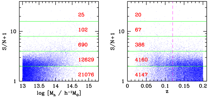
Figure 2: The $S/N$ ratios of X-ray clusters as a function of halo mass (left panel) and redshift (right panel). The number of X-ray clusters within each $S/N$ ratio bin (divided by the horizontal lines) is marked for reference (for all clusters in the left panel and for clusters with $z\leq 0.12$ in the right panel).

3 Measuring the X-ray luminosities of clusters from RASS imaging data

The main goal of this paper is to obtain the X-ray luminosities/signals around known optical clusters in the SDSS DR7 so that the resulting X-ray information can be used together with the optical information. In addition, this may enable us to obtain a larger X-ray cluster catalog with reliable X-ray detections from the RASS (see Wang et al. 2011 for a cross-identified 201 entries in the SDSS DR7 regions).

3.1 The X-ray luminosities around optical clusters

The algorithm we use to measure the X-ray luminosity is the same as in Shen at al. (2008), which is a modified version of the growth curve cluster detection method of Böhringer et al. (2000; 2004), and is referred to as the OTX (Optical to X-ray) code in the following. In our OTX detection algorithm, known information (e.g. $r_{200}$, $\sigma$, and the positions of the most massive galaxies) from the optical cluster catalog are extensively used. Here, we outline the main steps in the OTX code.

Step 1: Starting from a given optical cluster (with $\log M_{\rm h}\ga 13$), we sort the stellar masses of its member galaxies and find the most massive galaxies (MMGs). If the cluster has more than 4 member galaxies, we keep only 4 MMGs.

Step 2: For each cluster, we locate the RASS fields where its MMGs (up to 4) reside (Voges et al. 1999). We then apply a maximum likelihood (ML) detection algorithm on the RASS image of each of the fields and generate an X-ray source catalog which includes sources with detection likelihood $L>7$ in the 0.5-2.0 keV band (see Voges et al. 1999 for details). By matching X-ray sources within $0.3r_{200}$ from the MMGs, we determine the X-ray center of the cluster using the maximum X-ray emission density point (see Shen et al. 2008 for details). For those clusters without any X-ray emission density points that have likelihood $L>7$ detections, we use the MMG in consideration as the X-ray center.

Step 3: We mask out the ML detected sources that are not associated with the cluster. For example, the QSOs and stars cross-matched from RASS and SDSS-DR7 ($\sim 9200$) within $r_{200}$ from the X-ray center defined above are masked out (see Shen et al. 2008 for details). We then determine the X-ray background from an annulus centered on the X-ray center with an inner radius of $r_{200}$ and width of 6 arcmin. After subtracting the background, we generate a 1-dimensional source count rate profile and the corresponding cumulative source count rate profile as functions of radius. The X-ray extension radius is set as $r_{X}=0.5r_{200}$ (adopting smaller radius results in too few pixels for low-mass groups at high redshift). As we have tested by changing this value from $r_{X}=0.5r_{200}$ to $r_{X}=r_{200}$, none of our results are significantly impacted. Here we do not use the traditional (blind search) growth curve method in determining the $r_{X}$ (see Böhringer et al. 2000 for detail), as such a method may lead to bias due to the relatively high background in RASS.

Step 4: Calculate the X-ray luminosity $L_{\rm X}$. We integrate the source count rate profile inside $r_{X}$ and get the total source count rate of the cluster. We then assume that the X-ray emission has a thermal spectrum with a temperature $T$, and gas metal abundance of one third of the solar value to make a conversion from the source count rates to X-ray fluxes (and to X-ray luminosities according to the cosmology used in this paper). Finally, we make a $\beta$ profile extension correction to make up the X-ray luminosity missed in the range $r_{X}<r<r_{200}$ (see Böhringer et al. 2000; 2004; Shen et al. 2008). For each of the 4 MMGs, we calculate the related $L_{\rm X}$ following steps 2-4.

Step 5: Determine the central galaxy. We identify the central galaxy of the X-ray cluster from the 4 MMGs. If the values of $L_{\rm X}$ are different for the 4 MMGs, the central is defined to be the one that has $S/N>1.0$ and with the maximum $L_{\rm X}$. If more than one MMGs have $S/N>1.0$ and the difference of their $L_{\rm X}$ is less than the minimum of their $L_{\rm X}$ errors, we select the one that has the maximum $M_{\ast}^{1/3}/D_{p}$ as the central galaxy, where $M_{\ast}$ is the stellar mass of the candidate and $D_{p}$ is the projected distance between the candidate and the X-ray center. The factor $M_{\ast}^{1/3}/D_{p}$ used here is somewhat arbitrary but is a balance between the mass of the candidate galaxy and its distance to the X-ray center. We have tested that changing the power from $1/3$ to 0 or 1 yields results that are not significantly different. If none of the 4 MMGs has $S/N>1.0$, we assign the first MMGs as the central. Once the central galaxy is determined, we remove other MMGs and their associated measurements from our X-ray cluster list. Thus defined (chosen), the central galaxies are in general associated with the X-ray flux centriods.

We run our OTX code to search for X-ray signals around all 64,646 optical clusters with mass $\log M_{\rm h}\ga 13$. A total of 34,522 ($\sim 53\%$) of these clusters have a signal-to-noise ratio $S/N>0$ after subtracting the background signal. Here the signal-to-noise ratio on the X-ray cluster flux is calculated using

$${S/N}=\frac{R_{S}\,T}{\sqrt{R_{S}\,T+R_{B}\,T}},$$ (2)

(e.g. Henry et al. 2006), where $R_{S}$ is the source count rate in the aperture of radius $r_{200}$, $R_{B}$ is the background counting rate scaled to the aperture of radius $r_{200}$, and $T$ is the exposure time. These signal to noise ratios suffer from two problems: $(i)$ source confusion (projection effect): more than one cluster contribute to the X-ray emission within $0.5r_{200}$, causing the X-ray flux to be over-estimated, and $(ii)$ low $S/N$, especially for high redshift and low halo mass sources. To make maximal use of the X-ray information, we apply the following algorithm to address these two problems.

First for source confusion, quite a large fraction of X-ray clusters in our sample suffers from this projection effect. In order to keep the maximum number of X-ray clusters, we carry out the following X-ray luminosity division among the projected multi X-ray cluster systems. (1) For these systems, we make use of the average $L_{\rm X}$ - $M_{h}$ relation to obtain the ‘expected’ X-ray luminosities of the individual X-ray clusters. The average $L_{\rm X}$-$M_{h}$ relation is an important relation in probing cosmological parameters through the X-ray luminosity function of clusters, and has been extensively discussed and calibrated in the literature (e.g. Reiprich & Böhringer 2002; Stanek et al. 2006; Vikhlinin et al. 2009; Leauthaud et al. 2010; Arnaud et al. 2010; Mantz et al. 2010). Since we focus only on low-redshift ($0.01\leq z\leq 0.2$) X-ray clusters, with rest-frame X-ray luminosities measured in the broad ROSAT passband ($0.1$-$2.4$ keV), we use the $L_{\rm X}$-$M_{h}$ relation obtained by Mantz et al. (2010). By investigating the properties of 238 X-ray flux-selected galaxy clusters, Mantz et al. (2010) got the following X-ray luminosity-mass scaling relation which is free from Malmquist and Eddington biases,

$$\log\frac{L_{500\rm c}}{E(z)~{}10^{44}{\rm erg~{}s^{-1}}}=0.80+1.34~{}\log\frac{E(z)~{}M_{500\rm c}}{10^{15}M_{\odot}}\,,$$ (3)

and which has an intrinsic scatter $\sigma\sim 0.185$. In this relation, $E(z)=H(z)/H_{0}$, $M_{500\rm c}$ is the halo mass of the X-ray cluster within a radius $r_{500\rm c}$, defined as the radius within which the average mass density is $500$ times the critical mass density of the Universe, and $L_{500\rm c}$ is the total X-ray luminosity within $r_{500\rm c}$. Piffaretti et al. (2011) employed an iterative algorithm to calculate $L_{500\rm c}$ for sources with available aperture luminosities, and found $L_{500\rm c}/L_{\rm X}=0.91$. With this transformation, we obtain $M_{500\rm c}$ and $r_{500\rm c}$ for an X-ray cluster with given $L_{\rm X}$. The final step is then to convert $M_{500\rm c}$ to $M_{200}$, and $r_{500\rm c}$ to $r_{200}$ for consistency with our halo definition, i.e. the average overdensity is 200. Here we assume that dark matter halos follow a NFW density profile (Navarro et al. 1997) with concentration parameters given by the concentration-mass relation of Maccio et al. (2007). Based on this assumption, we have

$$r_{200} \simeq 2.70\times r_{500\rm c}\,,$$

$$M_{200} = M_{500\rm c}\times\frac{200}{500}\times\Omega_{\rm m}\times\left(\frac{r_{200}}{r_{500\rm c}}\right)^{3}\,.$$ (4)

Based on the above relations, we can obtain a rough estimate of the ‘expected’ average $L_{\rm X}$ for each cluster and the corresponding X-ray flux. (2) For multi-cluster systems, we add up all the ‘expected’ X-ray fluxes and obtain a contribution fraction for each cluster, ‘$i$’, in the system,

$$f_{mult,i}=F_{{\rm X},i}/\Sigma_{i}F_{{\rm X},i}\,.$$ (5)

This parameter is then applied to each cluster in the multi-cluster system to partly take into account the projection effect when quantities, such as $L_{\rm X}$ and $S/N$ are calculated.

Next, we check the $S/N$ of all the $34,522$ X-ray clusters with positive detections (i.e. positive count rates after background subtraction). Shown in the left and right panels of Fig. 2 are the $S/N$ distributions of these clusters in halo mass $M_{h}$ and in redshift $z$, respectively. For reference, we label the number of X-ray clusters within different $S/N$ bins. Among all the X-ray clusters, $817$ have $S/N>3$, $12,629$ have $3\geq S/N>1$, and $21,076$ have $1\geq S/N>0$. In a blind search for X-ray clusters, Henry et al. (2006) adopted $S/N=4$ as the threshold for reliable detection. Since here we are performing a counterpart detection, we take $S/N=3$ as our threshold for reliable X-ray detections, and sources with $S/N<3$ as tentative detections (see Wang 2004 for a detailed discussion about this detection threshold). The red squares in Fig 1 show the projected distribution of clusters with $S/N>3$.

3.2 Testing the performance of OTX using existing X-ray clusters

In order to test the reliability of our algorithm, we compare our measurements with X-ray clusters currently available in the literature. In a recent paper (Wang et al. 2011), we have performed the cross-identification between the SDSS DR7 groups and known X-ray cluster entries obtained from a variety of sources: the ROSAT Brightest Cluster Sample (BCS) and their low-flux extensions compiled by Ebeling et al. (1998, 2000), as well as the Northern ROSAT All-Sky (NORAS) and ROSAT-ESO Flux Limited X-ray (REFLEX) samples compiled by Böhringer et al. (2000, 2004). Within the same redshift and sky coverage of the SDSS DR7, we obtained an X-ray and optically matched catalog of 201 entries (see Appendix of Wang et al. 2011).

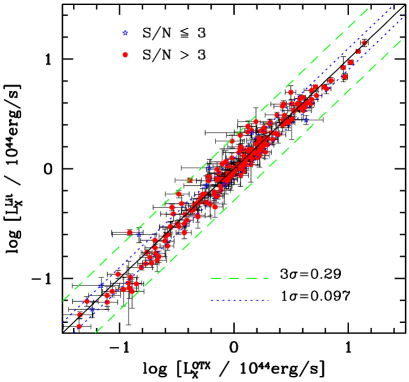
Figure 3: The X-ray luminosities of the cross-identified clusters, $\log L^{\rm Lit}_{\rm X}$, obtained from literature versus $\log L^{\rm OTX}_{\rm X}$ obtained by our OTX pipeline.

Before making any further investigation, we check if the X-ray luminosities of these clusters obtained from our OTX code are consistent with those given in the literature. We find that the vast majority of the 201 existing X-ray clusters are in our X-ray cluster sample with $S/N>3$. Three sources have $S/N\leq 3$ according to our OTX algorithm, mainly due to the shallow exposure of the RASS; in the literature they are detected by the PSPC and/or HRI point observations. Note that only 13 in our whole sample have $4\geq S/N>3$. Given the good cross detection, we consider our OTX clusters with $S/N>3$ to be reliable. Fig.3 shows the comparison between the X-ray luminosities obtained from literature compared to those obtained using the OTX code. The differences between them are almost negligible, and the luminosities obtained in these two ways are consistent with each other within the 1-$\sigma$ scatter of $0.097$ dex. Moreover, even the three clusters with $S/N\leq 3$ do not show large deviations. This test indicates again that our OTX code is reliable.

Within the SDSS DR7 sky coverage, our OTX pipeline extracts 817 X-ray clusters with $S/N>3$ with the help of optical data. Comparing to the existing 201 X-ray clusters, our new X-ray cluster sample is larger by a factor of almost 4. Including clusters with $3>S/N\geq 1$ further increases the sample size by another factor of $\sim 15$.

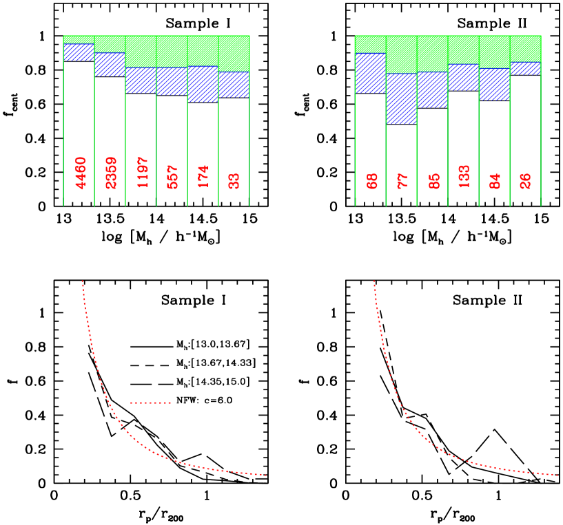
Figure 4: Shown in the upper panels are the accumulative fraction of central galaxies that are the MMGs, the second MMGs and others. Shown in the lower panels are the distributions of the projected distances between the MMGs and the central galaxies that are not MMGs. Here results are shown separately for samples I and II in the left and right panels, respectively.

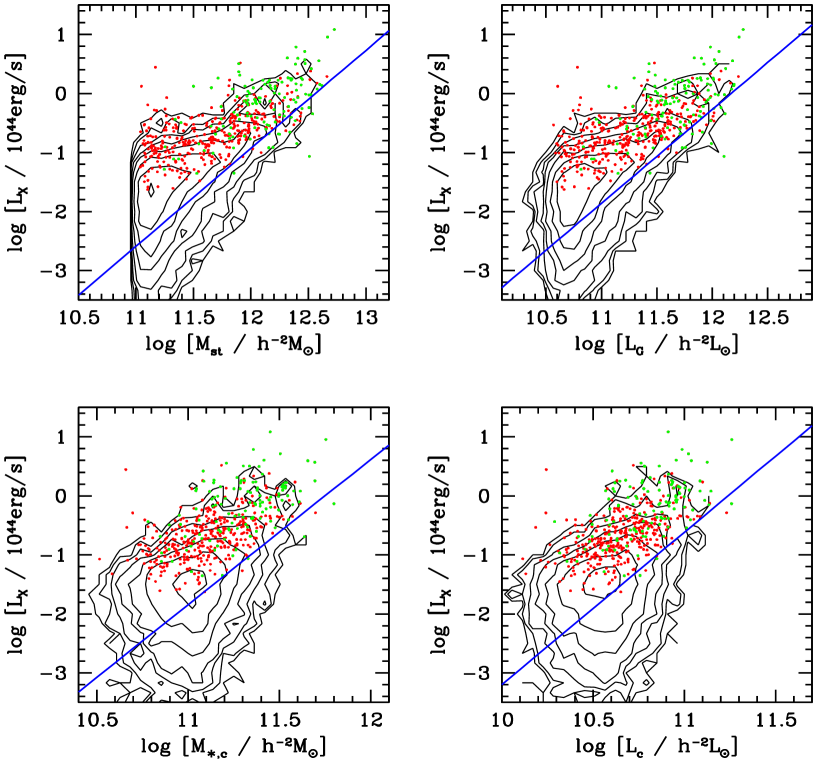
Figure 5: The correlation of X-ray cluster luminosity, $\log L_{\rm X}$, with the characteristic stellar mass (upper-left panel) and the cluster luminosity (upper-right panel), the stellar mass (lower-left panel) and luminosity (lower-right panel) of the MMG. Here results for sample I are shown as the black contours, while red dots are results for sample II. For comparison, we also show as green dots the results for the 131 X-ray clusters that are obtained from the literature with $z\leq 0.12$. The solid line in each panel is the best fit scaling relation (see text for details).

4 General properties of our X-ray clusters

Now that we have measured the X-ray luminosities for the optical clusters in SDSS DR7, we can proceed to examine various properties of these X-ray clusters. Because of observational limits both in X-ray and in optical, properties of clusters at higher redshift are expected to be less accurate. In particular the group catalog of Y07 was constructed based on galaxies brighter than $\>{}^{0.1}{\rm M}_{r}-5\log h=-19.5$, corresponding to a redshift $z\sim 0.1$ at the magnitude limit of the SDSS redshift survey. As a compromise between sample size and reliability, we only use clusters at $z<0.12$. Tests have shown that this redshift cut does not impact any of our results, other than increasing the scatter in some of the relations. Using the X-ray clusters with $z\leq 0.12$ we construct two samples for our investigation: sample I which contains $8,780$ clusters with $S/N>0$, and sample II which contains the subset of $473$ clusters with $S/N>3$. A comparison between these two samples can be used to test the reliability of the cluster detection.

4.1 Distances between the central and most massive galaxies in clusters

The central galaxy in a dark matter halo plays an important role in the theory of galaxy formation (e.g. Mo et al. 2010) as well as in our investigation of the dark matter distribution using galaxy-galaxy lensing measurement (e.g. Yang et al. 2006; Li et al. 2013). However, as dark matter is not directly observable, it is not straightforward to determine which galaxy is the true ‘central’ galaxy in a dark matter halo. In this paper we refer to the galaxy that is closest to the X-ray peak as the central galaxy. However, this center may deviate from that of the corresponding dark matter halo; in fact, in a few percent of cases, the central galaxy thus defined deviates from the X-ray peak position by up to a few arcminutes. These offsets are provided in our X-ray catalogue. An alternative method for defining the ‘central’ galaxy, is to associate it with the MMG (e.g. Yang et al. 2008). Once again, though, the location of the MMG may deviate significantly from that of the dark matter halo (e.g., Skibba et al. 2011). In this section, we examine the distribution of the separation between the two centers identified with these two definitions. Such information is useful in modelling the dark matter mass distribution around given clusters with galaxy-galaxy weak lensing measurements (e.g., Yang et al. 2006; Johnston et al. 2007; Sheldon et al. 2009; R. Li et al. 2013 in preparation; W. Luo et al., 2013 in preparation).

We first check the fraction of central galaxies in our X-ray cluster catalog that are the MMGs, the second MMGs and other ranks of member galaxies. As shown in the upper-left panel of Fig. 4 for sample I, the fraction of the MMGs that are central galaxies change from about 65% in very massive clusters to about 80% in relative low mass clusters. In $\sim 18\%$ of all the clusters, the central galaxies are the second most massive galaxies. As a reference, the total number of X-ray clusters in each halo mass bin is provided in the figure. Since the majority of our X-ray clusters have low $S/N$, the upper-right panel of Fig. 4 shows the same distribution, but for the X-ray clusters with $S/N>3$ (sample II). In this case, the fraction of central galaxies that are MMGs ranges from $\sim 50\%$ to $\sim 75\%$, with an average at $\sim 65\%$.

Next, we calculate the distances between the ‘centrals’ and the MMGs in our X-ray cluster sample. Note that here we only show results for central galaxies that are not the MMGs; for the majority cases, the distances are zero. In the lower-left panel of Fig. 4, we show the distribution of the projected distance, $r_{\rm p}$, obtained from all the X-ray clusters in sample I. Results are shown separately for clusters in different mass bins, as indicated, and the distance $r_{\rm p}$ is normalized by the virial radius of each cluster in question. For comparison, the dotted line shows the distribution expected for a projected NFW profile with concentration $c=6.0$. As one can see, the MMGs that are not central galaxies follows roughly a NFW profile. Although in general we are unable to determine whether the X-ray peak or the MMG traces the halo center better, the MMG fraction of centrals and the central-MMG distance distribution presented above can help us in separating weak lensing signal of centrals from that of satellites in a statistical sense (e.g., Johnston et al. 2007; W. Luo et al., 2013 in preparation; R. Li et al. 2013 in preparation).

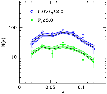
Figure 6: The redshift distributions of X-ray clusters within two different X-ray flux bins, as indicated using different symbols. For clarity, data for the low flux bin is shifted upward by a factor of 2. Error bars are obtained from 200 bootstrap resamplings of the clusters. The solid lines and shaded regions indicate the corresponding best fit model predictions and the 68% confidence levels.

4.2 X-ray - optical scaling relations

In this subsection, we examine the correlations of the X-ray luminosity $L_{\rm X}$ with a number of other properties obtained from the optical data: the characteristic stellar mass $M_{\rm st}$ and luminosity $L_{\rm G}$ of the cluster, the stellar mass and luminosity of the MMG, and the halo mass.

The upper panels of Fig. 5 show the correlation between cluster X-ray luminosity and characteristic stellar mass $M_{\rm st}$ (left panel) and luminosity $L_{\rm G}$ (right panel). Here contours show the results for sample I and dots for sample II. There is a clear trend that clusters with larger characteristic stellar masses and luminosities are more X-ray luminous. For a given characteristic stellar mass $M_{\rm st}$ or luminosity $L_{\rm G}$, the typical scatter in $\log L_{\rm X}$ is quite large: $\sim 0.40$ for sample II. To make sure that the scatter is not due to our OTX code, we show as green dots the results for the 131 X-ray clusters selected from the literature (Wang et al. 2011) applied with the same redshift cut $z\leq 0.12$. The fact that these 131 clusters show similar scatter suggests that this kind of scatter is likely intrinsic.

To obtain a rough guide to the relations between the X-ray and optical properties, we fit the observational results with

$$\log L_{\rm X}=a~{}(\log Y_{\rm opt}-b)\,,$$ (6)

where $Y_{\rm opt}=M_{\rm st}$ for characteristic stellar mass and $Y_{\rm opt}=L_{\rm G}$ for luminosity. In general, with reliable X-ray luminosity measurements for all the optical clusters, so that the sample is complete in $M_{\rm st}$ and $L_{\rm G}$, one could obtain directly a scaling relation as described by the above equation by fitting it into data. Unfortunately, in our X-ray sample, only about 21% of the objects have $S/N>1.0$. As pointed out in Stanek et al. (2006), using only a small fraction of reliably detected X-ray clusters (i.e. with high $S/N$) to obtain the scaling relations tend to systematically overestimate $L_{\rm X}$ for a given optical property due to the large intrinsic scatter in such a relation. This is caused by the combination of the Malmquist bias due to the fact that only X-ray luminous clusters are observed, and the Eddingtion bias owing to the fact X-ray fainter clusters are more abundant than X-ray brighter ones (see, e.g., Wang 2004; Stanek et al. 2006; Mantz et al. 2010). To alleviate the impact of such biases, we follow the method of Stanek et al. (2006) to constrain the two free parameters $a$ and $b$. This method uses the abundance of reliably detected X-ray clusters. To do this we obtain the number of clusters as a function of redshift in two X-ray flux bins. The results are shown in Fig. 6 using different symbols. Our test shows that the vast majority ($\ga 95\%$) of all the clusters with $F_{\rm X}\geq 2.0\times 10^{-12}{\rm erg~{}s^{-1}~{}cm^{-2}}$ have $S/N>1.0$.

We constrain the model parameters, $a$ and $b$, as follows. Starting from an initial guess of values of $a$ and $b$, we predict the median X-ray luminosity for each cluster using Eq. 6 from its $M_{\rm st}$ (or $L_{\rm G}$). Since the redshift range covered by the clusters is small, we ignore any possible evolution in the scaling relations. A log-normal dispersion is applied to the median X-ray luminosity. As pointed out in Stanek et al. (2006), the dispersion itself are not well constrained by the redshift distribution. We thus fix the dispersion, $\sigma_{L}=0.4$, according to that obtained directly from Sample II. We have tested that any change in the dispersion at the level of $\pm 50\%$ does not change any of our results significantly. The X-ray luminosities of all the clusters with redshift $z\leq 0.12$ obtained this way are converted into X-ray fluxes in the observed band taking into account the luminosity distances and negative average $K$ corrections based on the redshifts of individual clusters (Böhringer et al. 2004). A mock ‘X-ray cluster catalogue’ is then constructed, and we can calculate the redshift distributions of the mock clusters in different X-ray flux ranges, as shown in Fig. 6. These redshift distributions are then compared with those obtained directly from the observed sample to constrain the scaling relations. In practice we define a goodness-of-fit for each model using

$$\chi^{2}=\sum\left[{N(z)-\hat{N}(z)\over\Delta\hat{N}(z)}\right]^{2}\,,$$ (7)

where $\hat{N}$ and $\Delta\hat{N}$ are the observed average number and error, respectively. To explore the best fit values and the freedom of the model parameters, we follow Yan, Madgwick & White (2003; see also van den Bosch et al. 2005) and use a Monte-Carlo Markov Chain (hereafter MCMC) to explore the parameter space. We start our MCMC from an initial guess and allow a ‘burn-in’ of 1000 random walk steps for the chain to equilibrate in the parameter space. At each step in the chain we generate a new trial model by drawing the shifts in the free parameters from independent Gaussian distributions. The probability of accepting the trial model is assumed to be

$$P_{\rm accept}=\left\{\begin{array}[]{ll}1.0&\mbox{if $\chi^{2}_{\rm new}<\chi^{2}_{\rm old}$}\\ {\rm exp}[-(\chi^{2}_{\rm new}-\chi^{2}_{\rm old})/2]&\mbox{if $\chi^{2}_{\rm new}\geq\chi^{2}_{\rm old}$}\end{array}\right.$$ (8)

with $\chi^{2}$ given by eq. (7).

We construct a MCMC of $1$ million steps, with an average acceptance rate of $\sim 25\%$. We have tested its convergence using the ’convergence ratio’ $r$ as defined in Dunkley et al. (2005). In all cases $r<0.01$ is achieved for each parameter. To suppress the correlation between neighboring steps in the chain, we thin the chain by a factor of $100$. This results in a final MCMC consisting of $10,000$ independent models that sample the full posterior distribution. Among these models, we obtain the $68\%$ range of the best parameters with smaller $\chi^{2}$, and the best fit values are those with the smallest $\chi^{2}$ value. The resulting scaling relations for $M_{\rm st}$ and $L_{\rm G}$ are:

$$\log L_{\rm X} = 1.66^{+0.06}_{-0.17}~{}(\log M_{\rm st}-12.56^{+0.08}_{-0.03})\,,$$

$$\log L_{\rm X} = 1.59^{+0.16}_{-0.08}~{}(\log L_{\rm G}-12.17^{+0.04}_{-0.07})\,,$$ (9)

respectively, each of the quantities having the same units as in Fig. 5. Here the superscript and subscript of each parameter indicate the 68% confidence level. The best fit scaling relations are shown as the solid lines in the corresponding panels of Fig. 5. The scaling relations so obtained are steeper and smaller than those given directly by the small set of 473 X-ray clusters with $S/N>3$ which suffers from Malmquist and Eddingtion biases. The best fit redshift distributions of the X-ray clusters are shown as the solid lines in Fig. 6 in the corresponding X-ray flux ranges, with the shaded areas representing the 68 percentiles of the $10,000$ MCMC. Here results are shown only for $M_{\rm st}$, and the results are very similar for other optical quantities.

Next we investigate the correlation between the X-ray luminosity and the stellar mass $M_{\ast,c}$ (luminosity $L_{\rm c}$) of the central galaxy of a cluster. Here we refer to the most massive or brightest cluster galaxies as the central galaxies. The bottom row panels of Fig.  5 show these correlations, with $L_{\rm X}$-$M_{\ast,c}$ in the left-hand panel and $L_{\rm X}$-$L_{\rm c}$ in the right-hand panel. It is obvious that clusters with brighter X-ray luminosities on average have central galaxies that are more massive and more luminous. The scatter in $\log L_{\rm X}$ is similar to that shown in the upper panels for the characteristic stellar mass and luminosity. Using the same method as for $M_{\rm st}$ and $L_{\rm G}$, we fit Eq. (6) to the redshift distribution of X-ray clusters in the same three flux bins as shown Figure 6, and obtained the following scaling relations of $\log L_{\rm X}$ with $\log M_{\ast,c}$ and $\log L_{c}$:

$$\log L_{\rm X} = 2.46^{+0.18}_{-0.15}~{}(\log M_{\ast,c}-11.75^{+0.03}_{-0.03})\,,$$

$$\log L_{\rm X} = 2.58^{+0.12}_{-0.11}~{}(\log L_{c}-11.24^{+0.03}_{-0.04})\,.$$ (10)

These relations are shown as the solid lines in the bottom row panels of Fig. 5.

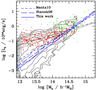
Figure 7: The X-ray cluster luminosity, $\log L_{\rm X}$, v.s. halo mass $\log M_{\rm h}$. The black contours show results for sample I, while red dots for sample II. For comparison, the green dots show the 131 X-ray clusters obtained from the literature with $z\leq 0.12$. The solid, long-dashed and dashed lines are the average $L_{\rm X}-M_{h}$ relations obtained in this work, by Stanek et al. (2006) and by Mantz et al. (2010), respectively. The dot-dashed and dotted lines are used to separate clusters with $S/N>3$ and $S/N>2$ into two subsamples with similar numbers of clusters.

We also investigate the correlation between the X-ray luminosity $L_{\rm X}$ and the halo mass, and the result is shown in Fig. 7. Although the scatter is large, in general $L_{\rm X}$ is positively correlated with $M_{h}$. In order to obtain an unbiased scaling relation between $\log L_{\rm X}$ and $\log M_{h}$, we proceed as follows. As pointed out in Yang et al. (2007), the typical scatter in halo mass estimation based on the ranking of $M_{\rm st}$ is about 0.3dex. In order to take such scatter into account we obtain a halo mass for each cluster with the following steps : (1) Start from a halo mass function and extract a list of ‘ture’ halo masses within the SDSS DR7 volume at redshift $z\leq 0.12$; (2) Add a log-normal deviation to each ‘true’ halo mass with 1-$\sigma$ scatter at 0.3 and obtain a ‘scattered’ halo mass; (3) Rank the ‘scattered’ halo masses and associate them to the ranks in $M_{\rm st}$; (4) Assign the‘true’ halo mass to each group according to the link between the true and ‘scattered’ masses. This approach gives a better model for the mass distribution of groups but not for the halo masses of individual groups. Finally, using the similar method as above, we fit to the redshift distribution of X-ray clusters, and obtain the best fit scaling relation between $\log L_{\rm X}$ and $\log M_{h}$,

$$\log L_{\rm X}=1.65^{+0.04}_{-0.02}~{}(\log M_{h}-14.70^{+0.01}_{-0.01})\,,$$ (11)

which is shown in Fig. 7 as the solid line. Our test shows that using the original assigned halo masses together with $\sigma_{L}=0.4$ for the X-ray luminosity, the resulting scaling relation is consistent Eq. 11 at the 2-$\sigma$ level. For comparison, the long-dashed and dashed lines in Fig. 7 show the average $L_{\rm X}-M_{h}$ relations obtained by Stanek et al. (2006) and Mantz et al. (2010), respectively. The scaling relation we get is in quite good agreement with these previous studies, especially with that obtained by Stanek et al. (2006).

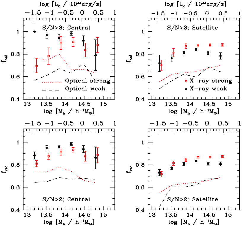
Figure 8: Upper panels: the red fraction of central (left) and satellite (right) galaxies in clusters with strong (squares) and weak (circles) X-ray emissions in Sample II (with $S/N>3$). Lower panels: similar to the upper panels but for clusters with $S/N>2$. The error bars are obtained from 200 bootstrap resamplings of all the clusters in question. For comparison, the dotted and dashed lines are results for ‘optically strong’ and ‘optically weak’ clusters, respectively. The related average $L_{\rm X}$ in each sample can be read from the top label of each panel. And for clarity, the red fraction is shifted downwards by a factor of 0.2.

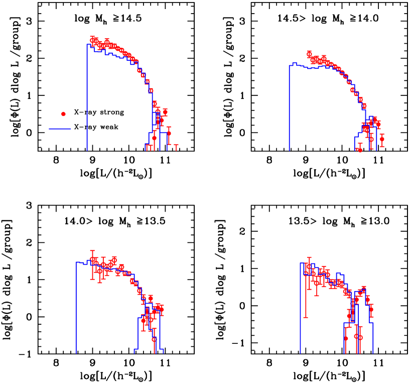
Figure 9: The conditional luminosity functions of clusters with strong (circles) and weak (histograms) X-ray emissions. The contribution of central and satellite galaxies are plotted separately. The error bars are obtained from 200 bootstrap resampling of all the clusters in question.

4.3 Galaxy properties in clusters of different X-ray luminosities

As demonstrated above, for given optical properties the cluster X-ray luminosities $L_{\rm X}$ have large variations (see also Castander et al. 1994; Lubin, Mulchaey & Postman 2004; Stanek et al. 2006; Popesso et al. 2007; Castellano et al. 2011; Balogh et al. 2011). The question is whether clusters of the same mass (or similar optical properties) but with different X-ray contents contain different galaxy populations. To shed light on this question, we divide our 473 X-ray clusters into 2 subsamples in the $L_{\rm X}$ - $M_{h}$ space in such a way that each subsample contains about half of the total number at a given $M_{h}$. The separation line is shown in Fig. 7 as the dot-dashed line. We refer clusters above and below the dividing line as “X-ray strong” and “X-ray weak”, respectively. We examine whether the galaxy populations in these two subsamples are different. We have checked various optical properties as a function of cluster mass for both these subsamples, including the stellar mass, $r$-band luminosity and concentration of the central galaxy, the stellar mass, velocity dispersion and luminosity gap (the magnitude difference between the first and second brightest galaxies) of member galaxies. None of these reveal any indication for a significant difference between X-ray strong and weak clusters.

An exception is the red fractions of central and satellite galaxies. The upper panels of Fig. 8 show the red fractions of central (left) and satellite (right) galaxies as a function of cluster mass, $M_{h}$, both for clusters with strong (open squares) and weak (open circles) X-ray emission in Sample II. Here galaxies have been split in red and blue populations, using the following magnitude-dependent color criterion:

$$^{0.1}(g-r)=9.97-0.0651\,x-0.00311\,x^{2}\,,$$ (12)

where $x=\>^{0.1}{\rm M}_{r}-5\log h+23.0$, which is similar to that used in Yang et al. (2008). Clusters with masses above and below $\sim 10^{14}\>h^{-1}\rm M_{\odot}$ reveal different behaviors. For $M_{h}\ga 10^{14}\>h^{-1}\rm M_{\odot}$, clusters with stronger X-ray emission have higher red satellite fraction: $\sim 90\%$ in X-ray strong clusters versus $\sim 80\%$ in X-ray weak clusters. This result is in quantitative agreement with the findings of Popesso et al. (2007) based on a significantly smaller sample of X-ray clusters. For clusters with $M_{h}\la 10^{14}\>h^{-1}\rm M_{\odot}$, the trend disappears in satellite galaxies but appears in central galaxies in an opposite direction. For $M_{h}\sim 10^{13}\>h^{-1}\rm M_{\odot}$, the red fraction of central galaxies in X-ray strong clusters is about 70%, much lower than that in X-ray weak clusters, which is $\sim 95\%$. To test the robustness of these results, we use a larger sample by adding clusters with lower $S/N$. The lower panels of Fig. 8 show the same results as the upper panels but for a total of 1193 clusters with $S/N>2$. Here the X-ray strong and X-ray weak clusters are separated using the dotted line shown in Fig.7, which splits the sample in subsamples that contain similar numbers of clusters at a given halo mass. Clearly, the general trend here is similar to that obtained using the smaller, higher-significance sample of clusters with $S/N>3$.

These results may indicate that there is a transition in the gas heating mechanism at a halo mass $\sim 10^{14}\>h^{-1}\rm M_{\odot}$. In lower mass clusters, the gas may be affected significantly by star formation and AGN activities in the central galaxies, which gives rise to the relative strong emission in X-ray as well as a relatively blue color. On the other hand, for clusters with masses above $\sim 10^{14}\>h^{-1}\rm M_{\odot}$, star formation in member galaxies may be more quenched if the amount of X-ray gas is larger. Alternatively, massive clusters with stronger X-ray emission may be more relaxed systems that assembled earlier and so their satellite galaxies formed earlier and also experienced longer time of star formation quenching.

To check the reliablity of our results, we carry out the following test. Since our halo masses are based on the ranks of $M_{\rm st}$, the separation in $L_{\rm X}$ of clusters in a given halo mass ($M_{h}$) range is the same as separation in a given $M_{\rm st}$ range. To check if and to what extent the findings of the red fraction described above are affected by uncertainties in the halo masses, let us consider the red fractions as a function of $L_{\rm X}$ instead of $M_{h}$. To this end, we first rank and separate our 473 X-ray clusters with $S/N>3.0$ (and 1193 clusters with $S/N>2.0$) into six $L_{\rm X}$ bins, each of which has exactly the same number of clusters as the corresponding $M_{h}$ bin. The clusters in each $L_{\rm X}$ bin are then divided into two subsamples, ‘optically strong’ and ‘optically weak’ according to the value of $M_{\rm st}$, so that the number of clusters in the ‘optically strong’ (‘optically weak’) subsample is the same as that in the ‘X-ray strong’ (‘X-ray weak) subsample. The corresponding results of the red fractions are shown in Fig. 8 using dotted and dashed lines. Here for clarity, the red fraction is shifted downwards by a factor of 0.2. As one can see, for satellite galaxies, the red fraction increases with $L_{\rm X}$, but for a given $L_{\rm X}$ it does not show any significant difference between the ‘optically strong’ and ‘optically weak’ subsamples. This is consistent with the results that satellite galaxies in ‘X-ray strong’ clusters of a given $M_{h}$ (or $M_{\rm st}$) on average have higher red fractions, and with the result that in clusters with $M_{h}>10^{14}\>h^{-1}\rm M_{\odot}$ the red fraction is quite independent of $M_{h}$ for both ‘X-ray strong’ and ‘X-ray weak’ clusters. For central galaxies, on the other hand, here we can see the red fraction in low $L_{\rm X}$ clusters does show significant difference between the ‘optically strong’ and ‘optically weak’ subsamples, in the sense that, for a given $L_{\rm X}$, the red fraction is higher for ‘optically strong’ clusters. The lower red fraction (or high blue fraction) of central galaxies in ‘optically weak’ clusters indicates that their relatively strong X-ray emission relative to their $M_{\rm st}$ may be due to high level of star formation, again in agreement with result that, for a given $M_{h}$ (or $M_{\rm st}$) in the low-mass end, ‘X-ray strong’ clusters on average have lower red fraction (higher blue fraction) than ‘X-ray weak’. With all these tests, we believe our results about the connection between star formation and X-ray strength is reliable.

Finally, we look at the conditional luminosity functions (CLF; see Yang, Mo & van den Bosch 2003) for these two subsamples of clusters. For this purpose we first divide the X-ray clusters into four mass bins. For each mass bin we determine the CLF using the same method as outlined in Yang et al. (2008). The results are shown in Fig. 9 as symbols with error bars for X-ray strong (filled for centrals, open for satellites) and as histograms for X-ray weak subsamples, respectively. Here the error bars have been obtained from 200 bootstrap re-samplings of all the clusters in question. Different panels correspond to different halo masses, as indicated by the value of $M_{h}$. Since the halo masses of clusters are estimated using $M_{\rm st}$ for all member galaxies with $\>{}^{0.1}{\rm M}_{r}-5\log h\leq-19.5$, the CLFs between the two samples at $\>{}^{0.1}{\rm M}_{r}-5\log h\leq-19.5$ are similar in both the central and satellite components. However, at the fainter end, a significant difference between the two subsamples is apparent in halos with masses $\ga 10^{14}\>h^{-1}\rm M_{\odot}$: clusters that are X-ray strong on average have more satellites than clusters of the same mass that are X-ray weak. In smaller halos with mass $\la 10^{14}\>h^{-1}\rm M_{\odot}$, such a difference disappears. We have also checked the CLFs separately for red and blue galaxies according to the color separation criterion given by Eq. (12). We find that the difference in the satellite CLFs between X-ray strong and weak massive clusters is mainly due to the excess of red galaxies in X-strong clusters, while the blue satellite galaxies have CLF that is quite independent of X-ray emission. This suggests that the excess of satellite galaxies in X-ray strong clusters is mainly due to survived satellites that were accreted earlier, rather than a larger fraction of galaxies transformed from blue to red galaxies. We have also checked the CLFs in different $L_{\rm X}$ bins separately for‘optically strong’ and ‘optically weak’ subsample, and found that ‘optically strong’ clusters have significantly higher CLFs than ‘optically weak’ clusters. This is expected by definition. We also found that the CLFs for the three highest $L_{X}$ bins are very similar.

5 Conclusions

Galaxy clusters are the largest known gravitationally bound objects. With their combined X-ray and optical properties (e.g. luminosities, masses, colors, etc.) understood, their power as cosmological constraints can be significantly increased. In addition, one can also take advantage of these combined properties to gain insight into the evolution of galaxies in the densest regions in the Universe.

Using an OTX code we developed and the ROSAT broadband ($0.1$-$2.4$ keV) archive, we have measured the X-ray luminosities around $\sim 65000$ optical clusters with masses $\ga 10^{13}\>h^{-1}\rm M_{\odot}$ identified from SDSS DR7. The optical information, such as the MMG positions, halo masses, are used in X-ray detections, which enables us to measure X-ray luminosities more reliably than without such information, as is shown by comparisons with X-ray clusters available from the literature. Among these clusters, 817 have $S/N>3$ X-ray detections, 12629 have $3\geq S/N>1$ and 21076 have $1\geq S/N>0$. Compared to the 201 entries available in the literature from the RASS in the SDSS DR7 coverage, our 817 clusters with $S/N>3$ already increase the number of detections by a factor of about 4.

Based on the 473 clusters with $S/N>3$ (sample II) and 8780 clusters with $S/N>0$ (sample I) at redshift $z\leq 0.12$, we have carried out some general analyses about the correlation between the X-ray luminosities and various optical properties of the clusters. Our main results are summarized as follows.

1. Among our X-ray clusters, about $65\%$ of the central galaxies, defined to be the galaxies nearest to the X-ray flux peak, are the MMGs in clusters. In the remaining $\sim 35\%$, the MMGs roughly follows a NFW profile with a concentration $c=6$ around the X-ray peaks.

2. The cluster X-ray luminosity shows correlation with the total stellar mass (or luminosity) of the clusters, and with the stellar mass of the central galaxy, but the scatter is quite large. The scaling relations we found are roughly at: $\log L_{\rm X}=1.66^{+0.06}_{-0.17}~{}(\log M_{\rm st}-12.56^{+0.08}_{-0.03})$; $\log L_{\rm X}=1.59^{+0.16}_{-0.08}~{}(\log L_{\rm G}-12.17^{+0.04}_{-0.07})$; $\log L_{\rm X}=2.46^{+0.18}_{-0.15}~{}(\log M_{\ast,c}-11.75^{+0.03}_{-0.03})$; $\log L_{\rm X}=2.58^{+0.12}_{-0.11}~{}(\log L_{c}-11.24^{+0.03}_{-0.04})$, with scatter $\sim 0.40$ in $\log L_{\rm X}$.

3. The scaling relation between X-ray luminosity and halo mass we obtained, $\log L_{\rm X}=1.65^{+0.04}_{-0.02}~{}(\log M_{h}-14.70^{+0.01}_{-0.01})$, is in quite good agreement with those obtained by Mantz et al. (2010) and Stanek et al. (2006).

4. Studying the galaxy populations in X-ray clusters of similar optical properties but different X-ray luminosities we found that, in massive halos with masses $\ga 10^{14}\>h^{-1}\rm M_{\odot}$, X-ray strong clusters have a larger fraction of red satellite galaxies, while the trend is absent in relative lower-mass halos.

5. In relative low mass halos with $M_{h}\la 10^{14}\>h^{-1}\rm M_{\odot}$, X-ray strong clusters have a smaller fraction of red central galaxies.

6. In massive clusters with masses $\ga 10^{14}\>h^{-1}\rm M_{\odot}$, strong X-ray emitters have many more low-mass satellite galaxies than weak X-ray emitters. Such a difference is absence in lower mass clusters.

7. The excess of these low-mass satellite galaxies in X-ray strong clusters is mainly due to red galaxies, suggesting that the excess of satellite galaxies in X-ray strong clusters is mainly due to survived satellites that were accreted earlier, rather than due to a larger fraction of galaxies transformed from blue to red galaxies.

References

- Abazajian et al. (2009) Abazajian, K. et al. , 2009, ApJS, 182, 534
- Arnaud et al. (2010) Arnaud, M., Pratt, G. W., Piffaretti, R., et al. 2010, A&A, 517A,92A
- Balogh et al. (2011) Balogh, M. L., Mazzotta, P., Bower, R. G., et al. 2011, MNRAS, 412, 947
- Berlind et al. (2006) Berlind, A. A., Frieman, J., Weinberg, D. H., et al. 2006, ApJS, 167, 1
- Blanton et al. (2005) Blanton, M. R., et al. 2005, AJ, 129, 2562
- Böhringer et al. (2000) Böhringer et al., 2000, ApJS, 129, 435
- Böhringer et al. (2004) Böhringer et al., 2004, A&A, 425, 367
- Böhringer et al. (2007) Böhringer et al., 2007, A&A, 469, 363
- Castander et al. (1994) Castander, F. J., Ellis, R. S., Frenk, C. S., Dressler, A., & Gunn, J. E. 1994, ApJ, 424, 79
- Castellano et al. (2011) Castellano, M., Pentericci, L., Menci, N., et al. 2011, A&A, 530, A27
- Choi et al. (2010) Choi, Y.Y., Han, D.H., Kim, S. S. 2010, JKAS, 43, 191-200
- Crook et al. (2007) Crook, A. C., Huchra, J. P., Martimbeau, N., et al. 2007, ApJ, 655, 790
- Dunkley et al. (2005) Dunkley, J., Bucher, M., Ferreira, P. G., Moodley, K., & Skordis, C. 2005, MNRAS, 356, 925
- Ebeling et al. (1998) Ebeling, H., Edge, A. C., Böhringer H., Allen, S. W., Crawford, C. S., Fabian, A. C., Voges, W., & Huchra, J. P. 1998, MNRAS, 301, 881
- Ebeling et al. (2000) Ebeling, H., Edge, A. C., Allen, S. W., Crawford, C. S., Fabian, A. C., & Huchra, J. P. 2000, MNRAS, 318, 333
- Einasto et al. (2007) Einasto, J., Einasto, M., Tago, E., et al. 2007, A&A, 462, 811
- Eke et al. (2004) Eke, V. R., Baugh, C. M., Cole, S., et al. 2004, MNRAS, 348, 866
- Forman et al. (1971) Forman, W., Kellogg, E., Gursky, H., Tananbaum, H., & Giacconi, R., 1971, ApJ, 138, 309
- Geller & Huchra (1983) Geller, M. J., & Huchra, J. P. 1983, ApJS, 52, 61
- Gerke et al. (2005) Gerke, B. F., Newman, J. A., Davis, M., et al. 2005, ApJ, 625, 6
- Goto (2005) Goto, T. 2005, MNRAS, 359, 1415
- Henry et al. (2006) Henry, J. P., Mullis, C. R., Voges, W., et al. 2006, ApJS, 162, 304
- Johnston et al. (2007) Johnston, D. E., Sheldon, E. S., Wechsler, R. H., et al. 2007, arXiv:0709.1159
- Kellogg et al. (1971) Kellogg E., Gurcky, H., Leong, C., Scherier, E., Tananbaum, H., & Giacconi, R., 1971, ApJ, 165, L49
- Lubin et al. (2004) Lubin, L. M., Mulchaey, J. S., & Postman, M. 2004, ApJ, 601, 9
- Maccio et al. (2007) Maccio, A. V., Dutton, A. A., van den Bosch, F. C., Moore, B., Potter, D., & Stadel, J. 2007, MNRAS, 378, 55
- Majumdar & Mohr (2004) Majumdar, S., & Mohr, J. J. 2004, ApJ, 613, 41
- Mantz et al. (2010) Mantz, A., Allen, S. W., Ebeling, H., Rapetti, D., & Drlica-Wagner, A. 2010, MNRAS, 406, 1773
- Merchán & Zandivarez (2002) Merchán, M., & Zandivarez, A. 2002, MNRAS, 335, 216
- Merchán & Zandivarez (2005) Merchán, M. E., & Zandivarez, A. 2005, ApJ, 630, 759
- Miller et al. (2005) Miller, C. J., Nichol, R. C., Reichart, D., et al. 2005, AJ, 130, 968
- Mo et al. (2010) Mo, H., van den Bosch, F. C., & White, S. 2010, Galaxy Formation and Evolution. Cambridge University Press, 2010. ISBN: 9780521857932,
- Navarro et al. (1997) Navarro, J. F., Frenk, C. S., & White, S. D. M. 1997, ApJ, 490, 493
- Piffaretti et al. (2011) Piffaretti, R., Arnaud, M., Pratt, G. W., Pointecouteau, E., & Melin, J.-B. 2011, A&A, 534, A109
- Popesso et al. (2007) Popesso, P., Biviano, A., Böhringer, H., & Romaniello, M. 2007, A&A, 461, 397
- Shen et al. (2008) Shen S., Kauffmann G., von der Linden A., White S. D. M., Best P.N., 2008, MNRAS, 389, 1074S
- Sheldon et al. (2009) Sheldon, E. S., Johnston, D. E., Scranton, R., et al. 2009, ApJ, 703, 2217
- Skibba et al. (2011) Skibba, R. A., van den Bosch, F. C., Yang, X., More, S., Mo, H., & Fontanot, F. 2011, MNRAS, 410, 417
- Stanek et al. (2006) Stanek, R., Evrard, A. E., Böhringer, H., Schuecker, P., Nord, B., 2006, ApJ, 648, 956
- Tago et al. (2006) Tago, E., Einasto, J., Saar, E., et al. 2006, Astronomische Nachrichten, 327, 365
- Tinker et al. (2008) Tinker, J., Kravtsov, A. V., Klypin, A., Abazajian, K., Warren, M., Yepes, G., Gottlöber, S., & Holz, D. E. 2008, ApJ, 688, 709
- Tucker et al. (2000) Tucker, D. L., Oemler, A., Jr., Hashimoto, Y., et al. 2000, ApJS, 130, 237
- van den Bosch et al. (2005) van den Bosch, F. C., Yang, X., Mo, H. J., & Norberg, P. 2005, MNRAS, 356, 1233
- Vikhlinin et al. (2009b) Vikhlinin, A., et al. 2009b, ApJ, 692, 1060
- Voges et al. (1999) Voges, W., et al. 1999, A&A, 349, 389
- Wang et al. (2011) Wang, L., Yang, X., Luo, W., et al. 2011, arXiv:1110.1987
- Wang (2004) Wang, Q. D. 2004, ApJ, 612, 159
- Weinmann et al. (2006) Weinmann, S. M., van den Bosch, F. C., Yang, X., & Mo, H. J. 2006, MNRAS, 366, 2
- Yan et al. (2003) Yan, R., Madgwick, D. S., & White, M. 2003, ApJ, 598, 848
- Yang et al. (2003) Yang X., Mo H.J., van den Bosch F.C., 2003, MNRAS, 339, 1057
- Yang et al. (2005) Yang X., Mo H.J., van den Bosch F.C., Jing Y.P., 2005, MNRAS, 356, 1293
- Yang et al. (2006) Yang, X., Mo, H. J., van den Bosch, F. C., et al. 2006, MNRAS, 373, 1159
- Yang et al. (2007) Yang X., Mo H.J., van den Bosch F.C., Pasquali A., Li C., Barden M., 2007, ApJ, 671, 153
- Yang et al. (2008) Yang X., Mo H.J., van den Bosch F.C., 2008, ApJ, 676, 248
- Yang et al. (2009) Yang X., Mo H. J., van den Bosch F. C., 2009, ApJ, 695, 900
- Yang et al. (2012) Yang, X., Mo, H. J., van den Bosch, F. C., Zhang, Y., & Han, J. 2012, ApJ, 752, 41