Non-Abelian photon

Abstract

In this paper, we have proposed $SU(2)$ non-Abelian electromagnetism gauge theory. In the theory, photon has self-interaction and interaction, which can explain photon entanglement phenomenon in quantum information. Otherwise, we find there are three kinds photons $\gamma^{+}$, $\gamma^{-}$ and $\gamma^{0}$, and they have electric charge $+e_{\gamma}$, $-e_{\gamma}$ and $0$, respectively, which are accordance with some experiment results.

Keywords: QED; SU(2) gauge theory

PACS: 11.15.-q, 12.20.-m

1 Introduction

The concept of photon as the quanta of the electromagnetic field dates back to the beginning of this century. In order to explain the spectrum of black-body radiation, Planck postulated the process of emission and absorption of radiation by atoms occurs discontinuously in quanta, i.e., the emission of black-body was energy quantization with value of $\hbar\omega$ [1], In 1905, Einstein had arrived at a more drastic interpretation. From a statistical analysis of the Planck radiation law and from the energetics of the photoelectric effect he concluded that it was not merely the atomic mechanism of emission and absorption of radiation which is quantized, but that electromagnetic radiation itself consists of photons. The Compton effect confirmed this interpretation.

The foundations of a systematic quantum theory of field were laid by Dirac in 1927. From the quantization of the electromagnetic field one is naturally led to the quantization of any classical field, the quanta of the field being particles with well-defined properties. We have successfully quantized the free Dirac electron, we would like to discuss the question of coupling the Dirac electron to a spin-one Maxwell field. The resulting theory had been called quantum electrodynamics, namely QED. Over the past decades, the quantum electrodynamics (QED) has attracted a considerable scientific attention [3, 4]. As we have already stated, QED is an Abelian gauge theory, which based on a $U(1)$ gauge symmetry. In 1954, Yang and Mills [5] extended the gauge principle to non-Abelian gauge symmetry, which based not on the simple one-dimensional group $U(1)$ of electrodynamics, but on a three-dimensional group, the group $SU(2)$ of isotopic spin conservation, in the hope that this would become a theory of the strong interactions. In particular, because the gauge group was non-Abelian there was a self-interaction of the gauge bosons, and the $U(1)$ Abelian gauge theory there was not a self-interaction.

Entanglement [6] is a unique feature of quantum theory having no analogue in classical physics. Spontaneous parametric down-conversion (SPDC) has been used as a source of entangled photon pairs for more than two decades [7] and provides an efficient way to generate non-classical states of light for fundamental tests of nature [8, 9], for quantum information processing [10, 11, 12] or for quantum metrology [13]. Entanglement between two photons emitted by SPDC can occur in one or several possible degrees of freedom of light [14], namely polarization, transverse momentum and energy. At present, the two-photon, three-photon and multi-photon entanglement have been observed in experiment [15, 16]. The photon entanglement is from photon self-interaction and the interaction among photons. In order to study the photon entanglement, we have extended the Abelian QED to the non-Abelian QED, which can describe the photon self-interaction and the interaction among photons.

In this paper, we have proposed $SU(2)$ non-Abelian electromagnetism gauge theory. In the theory, photon has self-interaction and interaction, which can explain photon entanglement phenomenon in quantum information. Otherwise, we find there are three kinds photons $\gamma^{+}$, $\gamma^{-}$ and $\gamma^{0}$, and they have electric charge $+e_{\gamma}$, $-e_{\gamma}$ and $0$, respectively, which are accordance with some experiment results.

2 QED with Abelian $U(1)$ gauge theory

In quantum theory, QED is an Abelian gauge theory. It is instructive to show that the theory ban be derived by the Dirac free electron theory to be gauge invariant and renormalizable. Consider the Lagrangian for a free electron field $\psi(x)$

$$L_{0}=\bar{\psi}(x)(i\gamma^{\mu}\partial_{\mu}-m)\psi(x),$$ (1)

the Dirac fields $\psi(x)$ and $\bar{\psi}(x)$ under the $U(1)$ local gauge transformations

$$\psi(x) \rightarrow\psi^{\prime-i\alpha(x)}\psi(x)$$

$$\bar{\psi}(x) \rightarrow\bar{\psi}^{\prime i\alpha(x)}\bar{\psi}(x)$$ (2)

where $\alpha(x)$ is a real number. The derivative term will now have a rather complicated transformation

$$\bar{\psi}(x)\partial_{\mu}\psi(x)\rightarrow\bar{\psi}^{\prime}(x)\partial_{\mu}\psi^{\prime}(x)=\bar{\psi}(x)\partial_{\mu}\psi(x)-i\bar{\psi}(x)\partial_{\mu}\alpha(x)\psi(x),$$ (3)

The second tern spoils the invariance. We need to form a gauge-covariant derivative $D_{\mu}$, to replace $\partial_{\mu}$, and $D_{\mu}\psi(x)$ will have the simple transformation

$$D_{\mu}\psi(x)\rightarrow[D_{\mu}\psi(x)]^{\prime-i\alpha(x)}D_{\mu}\psi(x),$$ (4)

so that the combination $\bar{\psi}(x)D_{\mu}\psi(x)$ is gauge invariant. In other words, the action of the covariant derivative on the field will not change the transformation property of the field. This can be realized if we enlarge the theory with a new vector field $A_{\mu}(x)$, the gauge field, and form the covariant derivative as

$$D_{\mu}\psi(x)=(\partial_{\mu}+ieA_{\mu})\psi(x),$$ (5)

where $e$ is a free parameter which we eventually will identify with electric charge. Then the transformation law for the covariant derivative (4) will be satisfied if the gauge field $A_{\mu}(x)$ has the transformation

$$A_{\mu}(x)\rightarrow A_{\mu}^{\prime}(x)=A_{\mu}(x)+\frac{1}{e}\partial_{\mu}\alpha(x),$$ (6)

Form (1) we now have

$$L=\bar{\psi}i\gamma^{\mu}(\partial_{\mu}+ieA_{\mu})-m\bar{\psi}\psi,$$ (7)

defining gauge field tensor $F_{\mu\nu}$ as

$$F_{\mu\nu}=\partial_{\mu}A_{\nu}-\partial_{\nu}A_{\mu},$$ (8)

under a transformation (6), the field tensor $F_{\mu\nu}$ is invariant, and we can structure the Lagrangian of $U(1)$ gauge field

$$L_{A}=-\frac{1}{4}F_{\mu\nu}F^{\mu\nu},$$ (9)

under a transformations (2) and (6), the invariant total Lagrangian of QED is

$$L=\bar{\psi}i\gamma^{\mu}(\partial_{\mu}+ieA_{\mu})\psi-m\bar{\psi}\psi-\frac{1}{4}F_{\mu\nu}F^{\mu\nu}.$$ (10)

The following features of (10) should be noted
(1) The photon is massless because a $A_{\mu}A^{\mu}$ term is not gauge invariant and not included in (10).
(2) The Lagrangian of (10) does not have a gauge field self-interaction.

3 QED with non-Abelian $SU(2)$ gauge theory

In 1954, Yang and Mills extended the gauge principle to non-Abelian symmetry, it is $SU(2)$ transformation group of isotopic spin. In order to study the photon entanglement, we have extended the Abelian QED to the non-Abelian QED. In the following, we shall study electromagnetism interaction with the $SU(2)$ gauge theory. We know electrons and positrons with the same mass and opposite charges which obey the same equation. The Dirac equation must therefore admit a new symmetry corresponding to the interchange particle and antiparticle. We thus seek a transformation $\psi\rightarrow\psi^{c}$ reversing the charge, and obtain the Dirac equations of electrons and positrons in electromagnetism field

$$[\gamma^{\mu}(\partial_{\mu}-ieA_{\mu})-m]\psi(x)=0,$$ (11)

and

$$[\gamma^{\mu}(\partial_{\mu}+ieA_{\mu})-m]{\psi}^{c}(x)=0,$$ (12)

where

$$\bar{\psi}^{c}(x)=\eta_{c}C\bar{\psi}^{T}(x),$$ (13)

$$C=i\gamma_{2}\gamma_{0}=\left(\begin{array}[c]{cc}0&-i\sigma_{2}\\ -i\sigma_{2}&0\end{array}\right),$$ (14)

where $\eta_{c}$ an arbitrary unobservable phase, generally taken as being equal to unity.

Let the fermion fields $\psi(x)$ and $\psi^{c}(x)$ of electrons and positrons be electric charge doublet of $SU(2)$

$$\psi=\left(\begin{array}[c]{c}\psi\\ \psi^{c}\end{array}\right).$$ (15)

For the scalar fields of electric charge, they are described by plural fields $\varphi(x)$ and $\varphi^{\ast}(x)$, the charge doublet of $SU(2)$ is

$$\psi=\left(\begin{array}[c]{c}\varphi\\ \varphi^{\ast}\end{array}\right).$$ (16)

For equation (15), under an $SU(2)$ transformation, we have

$$\psi(x)\rightarrow\psi^{{}^{\prime}}(x)=e^{-iT^{i}\cdot\theta^{i}}\psi(x),$$ (17)

where $T^{i}=\frac{1}{2}\sigma^{i}$, $\sigma^{i}(i=1,2,3)$ are the usual Pauli matrices, satisfying

$$[\frac{\sigma_{i}}{2},\frac{\sigma_{j}}{2}]=i\epsilon_{ijk}\frac{\sigma_{k}}{2}\hskip 21.68121pti,j,k=1,2,3,$$ (18)

and $\theta=(\theta_{1},\theta_{2},\theta_{3})$ are the $SU(2)$ transformation parameters. The free Lagrangian for electrons field $\psi(x)$

$$L_{0}={\bar{\psi}(x)}(i\gamma^{\mu}\partial_{\mu}-m)\psi(x),$$ (19)

is invariant under the global $SU(2)$ symmetry with ${\theta_{i}}$ being space-time independent. However, under the local symmetry transformation

$$\psi(x)\rightarrow\psi^{\prime}(x)=u(\theta)\psi(x),$$ (20)

with

$$u(\theta)=e^{-iT^{i}\cdot\theta^{i}(x)},$$ (21)

the free Lagrangian $L_{0}$ is no longer invariant because the derivative term transforms as

$$\bar{\psi}(x)\partial_{\mu}\psi(x)\rightarrow\bar{\psi}^{\prime}(x)\partial_{\mu}\psi^{\prime}(x)=\bar{\psi}(x)\partial_{\mu}\psi(x)+\bar{\psi}(x)u^{-1}(\theta)[\partial_{\mu}u(\theta)]\psi(x),$$ (22)

To construct a gauge-invariant Lagrangian we follow a procedure similar to that of the Abelian case. First we introduce three vector gauge fields $A_{\mu}^{i}$, $i=1,2,3$ (i.e., there are three kinds of photons) for the $SU(2)$ gauge group to form the gauge-covariant derivative through the minimal coupling

$$D_{\mu}(x)=\partial_{\mu}+A_{\mu}(x),$$ (23)

where

$$A_{\mu}(x)=-igA_{\mu}^{i}(x)T^{i},$$ (24)

where $g$ is the coupling constant in analogy to $e$ in (5). We demand that $D_{\mu}\psi$ have the same transformation property as $\psi$ itself, i.e.

$$D_{\mu}\psi\rightarrow(D_{\mu}\psi)^{\prime}=D_{\mu}^{\prime}\psi^{\prime}=D_{\mu}^{\prime}u(x)\psi=u(\theta)D_{\mu}\psi,$$ (25)

This implies that

$$(\partial_{\mu}-igT^{i}A_{\mu}^{\prime i})(u(\theta)\psi)=u(\theta)(\partial_{\mu}-igT^{i}A_{\mu}^{i})\psi,$$ (26)

or

$$[\partial_{\mu}u(\theta)-igT^{i}A_{\mu}^{\prime i}u(\theta)]=-igu(\theta)T^{i}A_{\mu}^{i},$$ (27)

or

$$T^{i}A_{\mu}^{\prime i}=u(\theta)T^{i}A_{\mu}^{i}u^{-1}(\theta)-\frac{i}{g}[\partial_{\mu}u(\theta)]u^{-1}(\theta),$$ (28)

which defines the transformation law for the gauge field. For an infinitesimal gauge change $\theta(x)\ll 1$,

$$u(\theta)\cong 1-i\vec{T}\cdot\vec{\theta}(x),$$ (29)

ignoring the higher order terms of $\theta^{j}$, equation (28) becomes

$$T^{i}A_{\mu}^{\prime i} =(1-iT^{j}\theta^{j})T^{i}A_{\mu}^{i}(1+iT^{j}\theta^{j})-\frac{i}{g}(-i\vec{T}\cdot\partial_{\mu}\vec{\theta})(1+i\vec{T}\cdot\vec{\theta})$$

$$=T^{i}A_{\mu}^{i}+iT^{i}A_{\mu}^{i}(T^{j}\theta^{j})-i(T^{j}\theta^{j})T^{i}A_{\mu}^{i}-\frac{1}{g}(\vec{T}\cdot\partial_{\mu}\vec{\theta}),$$

$$=T^{i}A_{\mu}^{i}+iA_{\mu}^{k}\theta^{j}T^{k}T^{j}-iA_{\mu}^{k}\theta^{j}T^{j}T^{k}-\frac{1}{g}(\vec{T}\cdot\partial_{\mu}\vec{\theta})$$

$$=T^{i}A_{\mu}^{i}-iA_{\mu}^{k}\theta^{j}[T^{j},T^{k}]-\frac{1}{g}(\vec{T}\cdot\partial_{\mu}\vec{\theta})$$

$$=T^{i}A_{\mu}^{i}+A_{\mu}^{k}\theta^{j}\epsilon^{ijk}T^{i}-\frac{1}{g}(\vec{T}\cdot\partial_{\mu}\vec{\theta})$$ (30)

or

$$A_{\mu}^{\prime i}=A_{\mu}^{i}+\epsilon^{ijk}A_{\mu}^{k}\theta^{j}-\frac{1}{g}\partial_{\mu}\theta^{i},$$ (31)

defining gauge field intensity $F_{\mu\nu}^{\alpha}$, it is

$$F_{\mu\nu}=D_{\mu}A_{\nu}-D_{\nu}A_{\mu}$$ (32)

and

$$F_{\mu\nu}=-igF_{\mu\nu}^{\alpha}T^{\alpha},$$ (33)

and

$$-igF_{\mu\nu}^{\alpha}T^{\alpha} =(\partial_{\mu}-igA_{\mu}^{\alpha}T^{\alpha})(-igA_{\nu}^{\beta}T^{\beta})-(\partial_{\nu}-igA_{\nu}^{\beta}T^{\beta})(-igA_{\mu}^{\alpha}T^{\alpha})$$

$$=-ig\partial_{\mu}A_{\nu}^{\beta}T^{\beta}+ig\partial_{\nu}A_{\mu}^{\alpha}T^{\alpha}-g^{2}A_{\mu}^{\alpha}A_{\nu}^{\beta}[T^{\alpha},T^{\beta}]$$

$$=-ig(\partial_{\mu}A_{\nu}^{\alpha}-\partial_{\nu}A_{\mu}^{\alpha})T^{\alpha}-ig^{2}\epsilon^{\alpha\beta\nu}A_{\mu}^{\alpha}A_{\nu}^{\beta}T^{\nu},$$ (34)

or

$$F_{\mu\nu}^{\alpha}=\partial_{\mu}A_{\nu}^{\alpha}-\partial_{\nu}A_{\mu}^{\alpha}+g\epsilon^{\alpha\beta\nu}A_{\mu}^{\beta}A_{\nu}^{\alpha}.$$ (35)

From equation (28), we have

$$A_{\mu}^{\prime}(x)=u(\theta)A_{\mu}(x)u^{-1}(\theta)+u(\theta)\partial_{\mu}u^{-1}(\theta),$$ (36)

$F_{\mu\nu}^{\prime}$ gauge transformation is

$$F_{\mu\nu}^{\prime} =D_{\mu}^{\prime}A_{\nu}^{\prime}-D_{\nu}^{\prime}A_{\mu}^{\prime}$$

$$=(\partial_{\mu}+A_{\mu}^{\prime})A_{\nu}^{\prime}-(\partial_{\nu}+A_{\nu}^{\prime})A_{\mu}^{\prime}$$

$$=(\partial_{\mu}+uA_{\mu}u^{-1}+u\partial_{\mu}u^{-1})(uA_{\nu}u^{-1}+u\partial_{\nu}u^{-1})$$

$$-(\partial_{\nu}+uA_{\nu}u^{-1}+u\partial_{\nu}u^{-1})(uA_{\mu}u^{-1}+u\partial_{\mu}u^{-1}),$$ (37)

the first term is

$$(\partial_{\mu}+uA_{\mu}u^{-1}+u\partial_{\mu}u^{-1})(uA_{\nu}u^{-1}+u\partial_{\nu}u^{-1})$$

$$=(\partial_{\mu}u)A_{\nu}u^{-1}+u(\partial_{\mu}A_{\nu})u^{-1}+uA_{\nu}(\partial_{\mu}u^{-1})+(\partial_{\mu}u)\partial_{\nu}u^{-1}+u\partial_{\mu}\partial_{\nu}u^{-1}$$

$$+uA_{\mu}u^{-1}uA_{\nu}u^{-1}+uA_{\mu}u^{-1}u\partial_{\nu}u^{-1}+u(\partial_{\mu}u^{-1})A_{\nu}u^{-1}+u(\partial_{\mu}u^{-1})u\partial_{\nu}u^{-1}$$

$$=u(\partial_{\mu}A_{\nu})u^{-1}+uA_{\nu}(\partial_{\mu}u^{-1})+u\partial_{\mu}\partial_{\nu}u^{-1}+uA_{\mu}A_{\nu}u^{-1}+uA_{\mu}\partial_{\nu}u^{-1}$$ (38)

and the second term is

$$(\partial_{\nu}+uA_{\nu}u^{-1}+u\partial_{\nu}u^{-1})(uA_{\mu}u^{-1}+u\partial_{\mu}u^{-1})$$

$$=u(\partial_{\nu}A_{\mu})u^{-1}+uA_{\mu}(\partial_{\nu}u^{-1})+u\partial_{\nu}\partial_{\mu}u^{-1}+uA_{\nu}A_{\mu}u^{-1}+uA_{\nu}\partial_{\mu}u^{-1}$$ (39)

substituting Eqs. (38) and (39) into (37), we have

$$F_{\mu\nu}^{\prime} =u[(\partial_{\mu}+A_{\mu})A_{\nu}-(\partial_{\nu}+A_{\nu})A_{\mu}]u^{-1}$$

$$=u(D_{\mu}A_{\nu}-D_{\nu}A_{\mu})u^{-1}$$

$$=uF_{\mu\nu}u^{-1},$$ (40)

under an infinitesimal gauge change (29), there is

$$F_{\mu\nu}\rightarrow F_{\mu\nu}^{\prime}=(1-iT^{a}\theta^{a})F_{\mu\nu}(1+iT^{b}\theta^{b}),$$ (41)

or

$$F_{\mu\nu}^{\prime c}T^{c} =(1-iT^{a}\theta^{a})F_{\mu\nu}^{c}T^{c}(1+iT^{b}\theta^{b})$$

$$=F_{\mu\nu}^{c}T^{c}+iF_{\mu\nu}^{c}T^{c}T^{b}\theta^{b}-iF_{\mu\nu}^{c}T^{a}T^{c}\theta^{a}+F_{\mu\nu}^{c}T^{a}T^{c}\theta^{a}T^{b}\theta^{b}$$

$$=F_{\mu\nu}^{c}T^{c}+iF_{\mu\nu}^{c}[T^{c},T^{b}]\theta^{b}$$

$$=F_{\mu\nu}^{c}T^{c}-\epsilon^{abc}F_{\mu\nu}^{a}T^{c}\theta^{b},$$ (42)

or

$$F_{\mu\nu}^{\prime c}=F_{\mu\nu}^{c}-\epsilon^{abc}F_{\mu\nu}^{a}\theta^{b},$$ (43)

i.e.,

$$F_{\mu\nu}^{\prime a}=F_{\mu\nu}^{a}-\epsilon^{cba}F_{\mu\nu}^{c}\theta^{b}=F_{\mu\nu}^{a}+\epsilon^{abc}F_{\mu\nu}^{c}\theta^{b}.$$ (44)

From equation (40), we have

$$F_{\mu\nu}^{\prime}F^{\mu\nu^{\prime}}=uF_{\mu\nu}u^{-1}uF^{\mu\nu}u^{-1}=uF_{\mu\nu}F^{\mu\nu}u^{-1},$$ (45)

and

$$TrF_{\mu\nu}^{\prime}F^{\mu\nu^{\prime}}=TruF_{\mu\nu}F^{\mu\nu}u^{-1}=TrF_{\mu\nu}F^{\mu\nu},$$ (46)

or

$$TrF_{\mu\nu}F^{\mu\nu^{\prime}} =Tr[(-igF_{\mu\nu}^{\alpha}T^{\alpha})(-igF^{\mu\nu\beta}T^{\beta})]$$

$$=-g^{2}F_{\mu\nu}^{\alpha}F^{\mu\nu\beta}Tr(T^{\alpha}T^{\beta})$$

$$=-\frac{1}{2}g^{2}F_{\mu\nu}^{\alpha}F^{\mu\nu\beta}\delta_{\alpha\beta}$$

$$=-\frac{1}{2}g^{2}F_{\mu\nu}^{\alpha}F^{\mu\nu\alpha},$$ (47)

the Lagrangian of gauge field can be taken as

$$L_{F}=-\frac{1}{4}F_{\mu\nu}^{\alpha}F^{\mu\nu\alpha},$$ (48)

and the total Lagrangian is

$$L =\bar{\psi}(i\gamma^{\mu}D_{\mu}-m)\psi-\frac{1}{4}F_{\mu\nu}^{\alpha}F^{\mu\nu\alpha}$$

$$=\bar{\psi}(i\gamma^{\mu}\partial_{\mu}-m)\psi-g\bar{\psi}\gamma^{\mu}A_{\mu}^{\alpha}T^{\alpha}\psi-\frac{1}{4}F_{\mu\nu}^{\alpha}F^{\mu\nu\alpha}.$$ (49)

The $U(1)$ and $SU(2)$ gauge theory of Abelian and non-Abelian have been introduced in many quantum field theory books [17, 18, 19]. In this paper, we apply the non-Abelian gauge theory to describe the electromagnetic interaction among photons, and obtain some new results:
(1) The photon is massless because a $A_{\mu}A^{\mu}$ term is not gauge invariant and not included in (49).
(2) The Lagrangian of (49) has a photon self-interaction, because of the term $\frac{1}{4}F_{\mu\nu}^{\alpha}F^{\mu\nu\alpha}$ in (49) contains products of three and four factors of $A_{\mu}$, and these imply diagrams of the three-photon vertex and four-photon vertex, which are shown in Fig. 1 (a) and (b).
(3) In $SU(2)$ gauge theory, there are three kinds photons $\gamma^{+}$, $\gamma^{-}$ and $\gamma^{0}$, they have three different electric charge $+e_{\gamma}$, $-e_{\gamma}$ and $0$, respectively. The electric charge quantity of photon is more less than the electric’s, i.e., $e_{\gamma}/e\ll 1$. In Refs. [20, 21, 22], these experiments have given the ratio of photon electric charge and electron electric charge $e_{\gamma}/e<3.4\times 10^{-5}$.

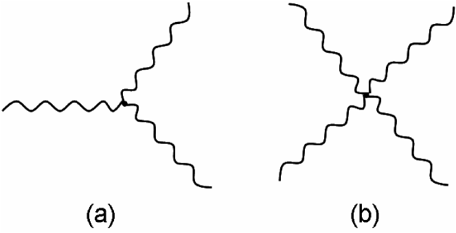
Figure 1: (a) three-photon vertex    (b) four-photon vertex

4 Conclusion

In this paper, we have proposed $SU(2)$ electromagnetism theory, which is the gauge theory of two-dimension electric charge space. In the theory, photon is massless, and it has self-interaction and interaction, i.e., there are three-photon and four-photon vertex. Otherwise, we find there are three kinds electric charge photons $\gamma^{+}$, $\gamma^{-}$ and $\gamma^{0}$. In some experiments, authors have found photon with teeny electric charge. We think the theory should be further tested by experiment.

References

- [1] M. Planck, The Theory of Heat Radiation, Philadel- phia, (1914).
- [2] A. Einstein, Concerning a Heuristic Point of View to-ward the Emission and Transformation of Light, Annals of Physics, Vol. 17, (1905).
- [3] A. Di Piazza, C. Muller, K.Z. Hatsagortsyan, and C.H. Kietel, Rev. Mod. Phys. 84, 1177 (2012).
- [4] V.I. Ritus, J. Sov. Laser Res. 6, 497 (1985).
- [5] C. N. Yang and R. L. Mills, Phys. Rev. 96, 191 (1954).
- [6] R. Horodecki, P. Horodecki, M. Horodecki and K. Horodecki, Rev. Mod. Phys. 81, 865 (2009).
- [7] R. Ghosh and L. Mandel, Phys. Rev. Lett. 59, 1903 (1987).
- [8] A. Zeilinger, Rev. Mod. Phys. 71, 288 ( 1999).
- [9] M. Genovese, Phys. Rep. 413, 319 (2005).
- [10] N. Gisin, G. Ribordy, W. Tittel and H. Zbinden, Rev. Mod. Phys. 74, 145 (2002).
- [11] N. Gisin and R. Thew, Nature Photonics 1, 165 (2007).
- [12] P. Kok, W. J. Munro, K. Nemoto, T. C. Ralph, J. P. Dowling and G. J. Milburn, Rev. Mod. Phys. 79, 135 (2007).
- [13] V. Giovannetti, S. Lloyd and L. Maccone, Nature Photonics 5, 222 (2011).
- [14] J. T. Barreiro, N. K. Langford, N. A. Peters and P. G. Kwiat Phys. Rev. Lett. 95, 260501 (2005).
- [15] D. Bouwmeester, J-W Pan, Phys. Rev. Lett, 82, 1345 (1999).
- [16] C. A. Sackett, Nature, 404, 256 (2000).
- [17] J. B. Bjorken and S. D. Drell. Relativistic Quantum Fields. Mc-Graw-Hill, (1965).
- [18] C. Itzykson and J. B. Zuber. Quantum Field Theory. Mc-Graw-Hill, (1980).
- [19] D. B. Lichtenberg, Unitary symmetry and elementary particles (2nd edn). Academic Press, New York. (1978).
- [20] M. I. Dobroliubov and A. Y. Ignatiev, Phys. Rev. Lett. 65, 679 (1990).
- [21] T. Mitsui, R. Fujimoto, Y. Ishisaki, Y. Ueda, Y. Yamazaki, S. Asai and S. Orito, Phys. Rev. Lett. 70, 2265 (1993).
- [22] A. Badertscher et al., Phys. Rev. D 75, 032004 (2007).