Correlation-based construction of neighborhood and edge features

Abstract

Motivated by an abstract notion of low-level edge detector filters, we propose a simple method of unsupervised feature construction based on pairwise statistics of features. In the first step, we construct neighborhoods of features by regrouping features that correlate. Then we use these subsets as filters to produce new neighborhood features. Next, we connect neighborhood features that correlate, and construct edge features by subtracting the correlated neighborhood features of each other. To validate the usefulness of the constructed features, we ran AdaBoost.MH on four multi-class classification problems. Our most significant result is a test error of $0.94\%$ on MNIST with an algorithm which is essentially free of any image-specific priors. On CIFAR-10 our method is suboptimal compared to today’s best deep learning techniques, nevertheless, we show that the proposed method outperforms not only boosting on the raw pixels, but also boosting on Haar filters.

1 Introduction

In this paper we propose a simple method of unsupervised feature construction based on pairwise statistics of features. In the first step, we construct neighborhoods of features by regrouping features that correlate. Then we use these subsets of features as filters to produce new neighborhood features. Next, we connect neighborhood features that correlate, and construct edge features by subtracting the correlated neighborhood features of each other. The method was motivated directly by the notion of low-level edge detector filters. These filters work well in practice, and they are ubiquitous in the first layer of both biological and artificial systems that learn on natural images. Indeed, the four simple feature construction steps are directly based on an abstract notion of Haar or Gabor filters: homogeneous, locally connected patches of contrasting intensities. In a more high-level sense, the technique is also inspired by a, perhaps naive, notion of how natural neural networks work: in the first layer they pick up correlations in stimuli, and settle in a “simple” theory of the world. Next they pick up events when the correlations are broken, and assign a new units to the new “edge” features. Yet another direct motivation comes from (Le Roux et al., 2007) where they show that pixel order can be recovered using only feature correlations. Once pixel order is recovered, one can immediately apply algorithms that explicitly use neighborhood-based filters. From this point of view, in this paper we show that it is possible to go from pixel correlations to feature construction, without going through the explicit mapping of the pixel order.

To validate the usefulness of the constructed features, we ran AdaBoost.MH (Schapire and Singer, 1999) on multi-class classification problems. Boosting is one of the best “shallow” multi-class classifiers, especially when the goal is to combine simple classifiers that act on small subsets a large set of possibly useful features. Within multi-class boosting algorithms, AdaBoost.MH is the state of the art. On this statement we are at odds with recent results on multiclass boosting. On the two UCI data sets we use in this paper (and on others reported in (Kégl and Busa-Fekete, 2009)), AdaBoost.MH with Hamming trees and products (Benbouzid et al., 2012) clearly outperforms SAMME (Zhu et al., 2009), ABC-Boost (Li, 2009), and most importantly, the implementation of AdaBoost.MH in (Zhu et al., 2009), suggesting that SAMME was compared to a suboptimal implementation of AdaBoost.MH in (Zhu et al., 2009).

Our most significant result comes on the MNIST set where we achieve a test error of $0.94\%$ with an algorithm which is essentially free of any image-specific priors (e.g., pixel order, preprocessing). On CIFAR-10, our method is suboptimal compared to today’s best deep learning techniques, reproducing basically the results of the earliest attempts on the data set (Ranzato et al., 2010). The main point in these experiments is that the proposed method outperforms not only boosting on the raw pixels, but also boosting on Haar filters. We also tried the technique on two relatively large UCI data sets. The results here are essentially negative: the lack of correlations between the features do not allow us to improve significantly on “shallow” AdaBoost.

The paper is organized as follows. In Section 2 we formally describe the method. In Section 3 we show experimental results, and we conclude with a discussion on future research in Section 4.

2 Constructing the representation

For the formal description of the method, let ${\cal D}=\big{\{}({\bf x}_{1},y_{1}),\ldots,({\bf x}_{n},y_{n})\big{\}}$ the training data, where ${\bf x}_{i}=(x_{i}^{1},\ldots,x_{i}^{d})\in{\mathbb{R}}^{d}$ are the input vectors and $y_{i}\in\{1,\ldots,K\}$ the labels. We will denote the input matrix and its elements by ${\cal X}=[x_{i}^{j}]_{i=1,\ldots,n}^{j=1,\ldots,d}$, and its raw feature (column) vectors by ${\bf x}^{j}=(x_{1}^{j},\ldots,x_{n}^{j})\in{\mathbb{R}}^{n}$. The algorithm consists of the following steps.

1. We construct neighborhoods $J({\bf x}^{j})$ for each feature vector ${\bf x}^{j}$, that is, sets of features that are correlated with ${\bf x}^{j}$. Formally, $J({\bf x}^{j})=\{j^{\prime}:{\bf x}^{j^{\prime}}\in{\cal X}:\rho({\bf x}^{j},{\bf x}^{j^{\prime}})<\rho_{\text{N}}\}$, where

   $$\rho({\bf x}^{j},{\bf x}^{j^{\prime}})=\frac{{{\mathrm{Cov}}\left\{{{\bf x}^{j},{\bf x}^{j^{\prime}}}\right\}}}{\sqrt{{{\mathrm{Var}}\left\{{{\bf x}^{j}}\right\}}{{\mathrm{Var}}\left\{{{\bf x}^{j^{\prime}}}\right\}}}}$$

   is the correlation of two feature vectors and $\rho_{\text{N}}$ is a hyperparameter of the algorithm.

2. We construct neighborhood features by using the neighborhoods as (normalized) filters, that is,

   $$z_{i}^{j}=\frac{1}{|J({\bf x}^{j})|}\sum_{j^{\prime}\in J({\bf x}^{j})}x_{i}^{j^{\prime}}$$

   for all $i=1,\ldots,n$ and $j=1\ldots,d$.

3. We construct edges between neighborhoods by connecting correlated neighborhood features. Formally, ${\cal L}=\{(j_{1},j_{2}):1\leq j_{1},j_{2}\leq d,\;\rho({\bf z}^{j_{1}},{\bf z}^{j_{2}})<\rho_{\text{E}}\}$, where $\rho_{\text{E}}$ is a hyperparameter of the algorithm. We will denote elements of the set of edges by $(\ell_{j,1},\ell_{j,2})$, and the size of the set by $|{\cal L}|=L$.

4. We construct edge features by subtracting the responses to correlated neighborhoods of each other, that is, $s_{i}^{j}=z_{i}^{\ell_{j,1}}-z_{i}^{\ell_{j,2}}$ for all $j=1,\ldots,L$ and $(\ell_{j,1},\ell_{j,2})\in{\cal L}$.

5. We concatenate neighborhood and edge features into a new representation of ${\bf x}_{i}$, that is, ${\bf x}^{\prime}_{i}=\big{(}z_{i}^{1},\ldots,z_{i}^{d},s_{i}^{1},\ldots,s_{i}^{L}\big{)}$ for all $i=1,\ldots,n$.

2.1 Setting $\rho_{\text{N}}$ and $\rho_{\text{E}}$

Both hyperparameters $\rho_{\text{N}}$ and $\rho_{\text{E}}$ threshold correlations, nevertheless, they have quite different roles: $\rho_{\text{N}}$ controls the neighborhood size whereas $\rho_{\text{E}}$ controls the distance of neighborhoods under which an edge (that is, a significantly different response or a “surprise”) is an interesting feature. In practice, we found that the results were rather insensitive to the value of these parameters in the $[0.3,0.9]$ interval. For now we manually set $\rho_{\text{N}}$ and $\rho_{\text{E}}$ in order to control the number of features. In our experiments we found that it was rarely detrimental to increase the number of features in terms of the asymptotic test error (w.r.t. the number of boosting iterations $T$) but the convergence of AdaBoost.MH slowed down if the number of features were larger than some thousands (either because each boosting iteration took too much time, or because we had to seriously subsample the features in each iteration, essentially generating random trees, and so the number of iterations exploded).

On images, where the dimensionality of the input space (number of pixels) is large, we subsample the pixels $[{\bf x}^{j}]_{j=1,\ldots,d}$ before constructing the neighborhoods $J({\bf x}^{j})$ to control the number of neighborhood features, again, for computational rather than statistical reasons. We simply run AdaBoost.MH with decision stumps in an autoassociative setup. A decision stump uses a single pixel as input and outputs a prediction on all the pixels. We take the first $d^{\prime}$ stumps that AdaBoost picks, and use the corresponding pixels (a subset of the full set of pixels) to construct the neighborhoods.

On small-dimensional (non-image) sets we face the opposite problem: the small number of input features limit the number of neighborhoods. This actually highlights a limitation of the algorithm: when the number of input features is small and they are not very correlated, the number of generated neighborhood and edge features is small, and they essentially contain the same information as the original features. Nevertheless, we were curious whether we can see any improvement by blowing up the number of features (similarly, in spirit, to what support vector machines do). We obtain a larger number of neighborhoods by defining a set of thresholds $\{\rho_{\text{N}}^{1},\ldots,\rho_{\text{N}}^{M}\}$, and constructing $M$ “concentric” neighborhoods for each feature ${\bf x}^{j}$. On data sets with heterogeneous feature types it is also important to normalize the features by the usual transformation ${x^{j}_{i}}^{\prime}=\big{(}x^{j}_{i}-\mu({\bf x}^{j})\big{)}/\sigma({\bf x}^{j})$, where $\mu({\bf x})$ and $\sigma({\bf x})$ denote the mean and the standard deviation of the elements of ${\bf x}$, respectively, before proceeding with the feature construction (Step 2).

Optimally, of course, automatic hyperparameter optimization (Bergstra and Bengio, 2012; Bergstra et al., 2011; Snoek et al., 2012) is the way to go, especially since AdaBoost.MH also has two or three hyperparameters, and manual grid search in a four-to-five dimensional hyperparameter space is not feasible. For now, we set aside this issue for future work.

2.2 AdaBoost.MH with Hamming trees

The constructed features can be input to any “shallow” classifier. Since we use AdaBoost.MH with Hamming trees, we briefly describe them here. The full formal description with the pseudocode is in the documentation of MultiBoost (Benbouzid et al., 2012). It is available at the multiboost.org website along with the code itself.

The advantage of $\Algo{AdaBoost.MH}$ over other multi-class boosting approaches is that it does not require from the base learner to predict a single label $\widehat{y}=h({\bf x})$ for an input instance ${\bf x}$, rather, it uses vector-valued base learners ${\bf h}({\bf x})$. The requirement for these base learners is weaker: it suffices if the edge $\gamma({\bf h},{\bf W})=\sum_{i=1}^{n}\sum_{\ell=1}^{K}w_{i,\ell}h_{\ell}(x_{i})y_{i,\ell}$ is slightly larger than zero, where ${\bf W}=[w_{i,\ell}]_{i=1,\ldots,n}^{\ell=1,\ldots,K}$ is the weight matrix (over instances and labels) in the current boosting iteration, and ${\bf y}_{i}=(y_{i,1},\ldots,y_{i,K})$ is a $\pm 1$-valued one-hot code of the label. This makes it easy to turn weak binary classifiers into multi-class base classifiers, without requiring that the multi-class zero-one base error be less than $1/2$. In case ${\bf h}$ is a decision tree, there are two important consequences. First, the size (the number of leaves $N$) of the tree can be arbitrary and can be tuned freely (whereas requiring a zero-one error to be less than $1/2$ usually implies large trees). Second, one can design trees with binary $\{\pm 1\}^{K}$-valued outputs, which could not be used as standalone multi-class classifiers.

In a Hamming tree, at each node, the split is learned by a multi-class decision stump of the form ${\bf h}({\bf x})={\bf v}\varphi({\bf x})$, where $\varphi({\bf x})$ is a (standard) scalar $\pm 1$-valued decision stump, and ${\bf v}$ is a $\{\pm 1\}^{K}$-valued vector. At leaf nodes, the full $\{\pm 1\}^{K}$-valued vector ${\bf v}\varphi({\bf x})$ is output for a given ${\bf x}$, whereas at inner nodes, only the binary function $\varphi({\bf x})$ is used to decide whether the instance ${\bf x}$ goes left or right. The tree is constructed top-down, and each node stump is optimized in a greedy manner, as usual. For a given ${\bf x}$, unless ${\bf v}$ happens to be a one-hot vector, no single class can be output (because of ties). At the same time, the tree is perfectly boostable: the weighted sum of Hamming trees produces a real-valued vector of length $K$, of which the predicted class can be easily derived using the $\mathop{\rm arg\,max}$ operator.

3 Experiments

We carried out experiments on four data sets: MNIST and CIFAR-10 are standard image classification data sets, and the Pendigit and Letter sets are relatively large benchmarks from the UCI repository. We boosted Hamming trees (Benbouzid et al., 2012) on each data sets. Boosted Hamming trees have three hyperparameters: the number of boosting iterations $T$, the number of leaves $N$, and the number of (random) features $d^{\prime}$ considered at each split (LazyBoost (Escudero et al., 2000) settings that give the flavor of a random forest to the final classifier). Out of these three, we validated only the number of leaves $N$ in the ‘‘classical’’ way using $80/20$ single validation on the training set. Since AdaBoost.MH does not exhibit any overfitting even after a very large number of iterations (see Figure 1), we run it for a large number of $T=10^{5}$ iterations, and report the average test error of the last $T/2$ iterations. The number of (random) features $d^{\prime}$ considered at each split is another hyperparameter which does not have to be tuned in the traditional way. In our experience, the larger it is, the smaller the asymptotic test error is. On the other hand, the larger it is the slower the algorithm converges to this error. This means that $d^{\prime}$ controls the trade-off between the accuracy of the final classifier and the training time. We tuned it to obtain the full learning curves in reasonable time.

The neighborhood and edge features were constructed as described in Section 2. Estimating correlations can be done robustly on relatively small random samples, so we ran the algorithm on a random input matrix ${\cal X}$ with $1000$ instances.

3.1 MNIST

MNIST consists of $60000$ grey-scale training images of hand-written digits of size $28\times 28=784$. In all experiments on MNIST, $d^{\prime}$ was set to $100$. The first baseline run was AdaBoost.MH with Hamming trees of $8$ leaves on the raw pixels (green curve in Figure 1(a)), achieving a test error of $1.25\%$. We also ran AdaBoost.MH with Hamming trees of $8$ leaves in the roughly $300000$-dimensional feature space generated by five types of Haar filters (Viola and Jones 2004; red curve in Figure 1(a)). This setup produced a test error of $0.85\%$ which is the state of the art among boosting algorithms. For generating neighborhood and edge features, we first ran autoassociative AdaBoost.MH with decision stumps for $800$ iterations that picked the $326$ pixels depicted by the white pixels in Figure 2(a). Then we constructed $326$ neighborhood features using $\rho_{\text{N}}=0.5$ and $1517$ edge features using $\rho_{\text{E}}=0.7$. The $100$ most important features (picked by running AdaBoost.MH with decision stumps) is depicted in Figure 3. Finally we ran AdaBoost.MH with Hamming trees of $8$ leaves on the constructed features (blue curve in Figure 1(a)), achieving a test error of $0.94\%$ which is one of the best results among methods that do not use explicit image priors (pixel order, specific distortions, etc.).

Note that AdaBoost.MH picked slightly more neighborhood than edge features relatively to their prior proportions. On the other hand, it was crucial to include both neighborhood and edge features: AdaBoost.MH was way suboptimal on either subset.

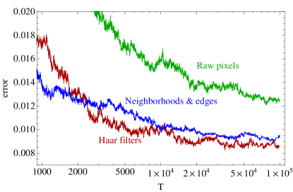
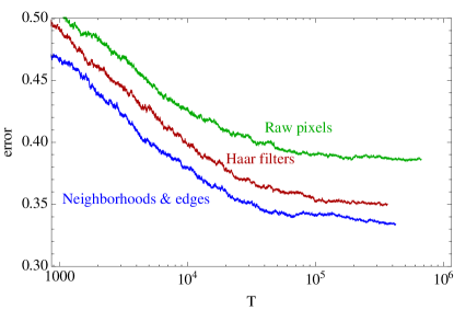
(a) MNIST (b) CIFAR-10

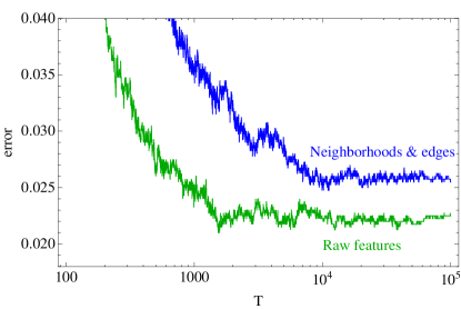
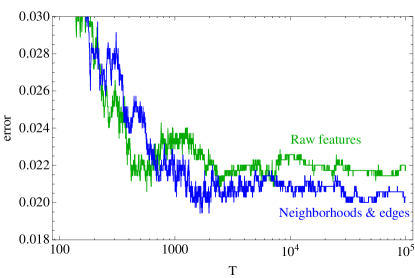
(c) UCI Letter (d) UCI Pendigit

Figure 1: Test learning curves.

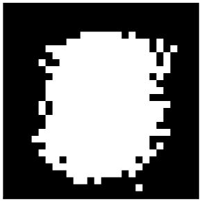
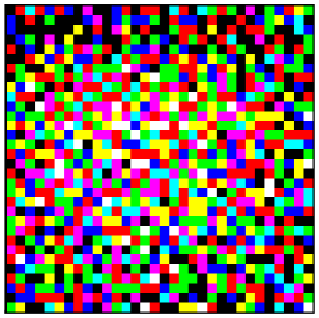
(a) MNIST (b) CIFAR-10

Figure 2: Initial pixel selection using autoassociative AdaBoost.MH. (a) White means that the pixel is selected, black means it is not. (b) Colors are mixtures of the color channels selected. White means that all channels were selected, and black means that none of them were selected.

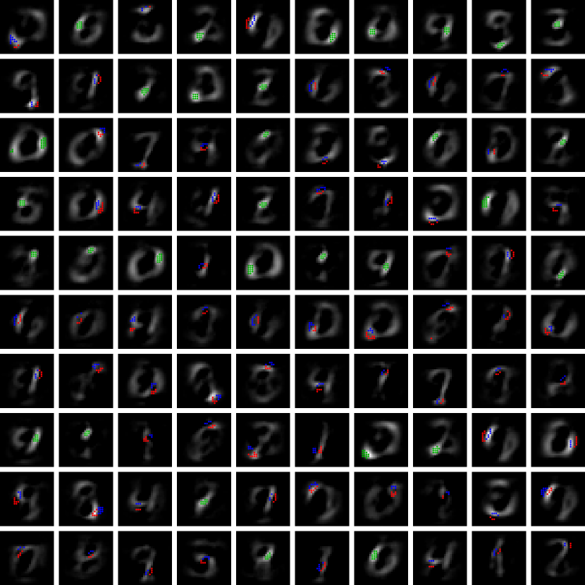
Figure 3: The $100$ most important neighborhood and edge features picked by AdaBoost.MH. In neighborhood features we mark the middles of pixels in the neighborhood $J({\bf x}^{j})$ by green dots. In edge features we mark the middles of pixels of the positive neighborhood by blue dots, and the pixels of the negative neighborhood by red dots. The black&white images in both cases are averages of the 20% of MNIST test images that respond the strongest to the given filter.

3.2 CIFAR

CIFAR-10 consists of $50000$ color training images of 10 object categories of size $32\times 32=1024$, giving a total of $3\times 1024=3072$ features. In all experiments on CIFAR, $d^{\prime}$ was set to $10$. The first baseline run was AdaBoost.MH with Hamming trees of $20$ leaves on the raw pixels (green curve in Figure 1(b)), achieving a test error of $39.1\%$. We also ran AdaBoost.MH with Hamming trees of $20$ leaves in the roughly $350000$-dimensional feature space generated by five types of Haar filters (Viola and Jones 2004; red curve in Figure 1(b)). This setup produced a test error of $36.1\%$. For generating neighborhood and edge features, we first ran autoassociative AdaBoost.MH with decision stumps for $1000$ iterations that picked the $922$ color channels depicted by the white and colored pixels in Figure 2(b). Then we constructed $922$ neighborhood features using $\rho_{\text{N}}=0.85$ and $4552$ edge features using $\rho_{\text{E}}=0.85$. Finally we ran AdaBoost.MH with Hamming trees of $20$ leaves on the constructed features (blue curve in Figure 1(a)), achieving a test error of $33.6\%$.

None of these results are close to the sate of the art, but they are not completely off the map, either: they match the performance of one of the early techniques that reported error on CIFAR-10 (Ranzato et al., 2010). The main significance of this experiment is that AdaBoost.MH with neighborhood and edge features can beat not only AdaBoost.MH on raw pixels but also AdaBoost.MH with Haar features.

3.3 UCI Pendigit and Letter

In principle, there is no reason why neighborhood and edge features could not work on non-image sets. To investigate, we ran some preliminary tests on the relatively large UCI data sets, Pendigit and Letter. Both of them contain $16$ features and several thousand instances. The baseline results are $2.16\%$ on Pendigit using AdaBoost.MH with Hamming trees of $4$ leaves (green curve in Figure 1(d)) and $2.23\%$ on Letter using AdaBoost.MH with Hamming trees of $20$ leaves (green curve in Figure 1(c)). We constructed neighborhoods using a set of thresholds $\rho_{\text{N}}=\{0.1,0.2,\ldots,0.9\}$, giving us $62$ unique neighborhoods on Letter and $86$ unique neighborhoods on Pendigit (out of the possible $9\times 16=126$). We then proceeded by constructing edge features with $\rho_{\text{E}}=0.7$, giving us $506$ more features on Letter, and $1040$ more features on Letter. We then ran AdaBoost.MH with Hamming trees of the same number of leaves as in the baseline experiments, using $d^{\prime}=100$. On Pendigit, we obtained $2.05\%$, better than in the baseline (blue curve in Figure 1(d)), while on Letter we obtained $2.59\%$, significantly worse than in the baseline (blue curve in Figure 1(c)). We see two reasons why a larger gain is difficult on these sets. First, there is not much correlation between the features to exploit. Indeed, setting $\rho_{\text{N}}$ and $\rho_{\text{E}}$ to similar values to those we used on the image sets, neighborhoods would have been very small, and there would have been almost no edges. Second, AdaBoost.MH with Hamming trees is already a very good algorithm on these sets, so there is not much margin for improvement.

4 Future work

Besides running more experiments and tuning hyperparameters automatically, the most interesting question is whether stacking neighborhood and edge features would work. There is no technical problem of re-running the feature construction on the features obtained in the first round, but it is not clear whether there is any more structure this simple method can exploit. We did some preliminary trials on MNIST where it did not improve the results, but this may be because MNIST is a relatively simple set with not very complex features and rather homogeneous classes. Experimenting with stacking on CIFAR is definitely the next step. Another interesting avenue is to launch a large scale exploration on more non-image benchmark sets to see whether there is a subclass of sets where the correlation-based feature construction may work, and then to try to characterize this subclass.

References

- Benbouzid et al. (2012) Benbouzid, D., Busa-Fekete, R., Casagrande, N., Collin, F.-D., and Kégl, B. (2012). MultiBoost: a multi-purpose boosting package. Journal of Machine Learning Research, 13, 549--553.
- Bergstra and Bengio (2012) Bergstra, J. and Bengio, Y. (2012). Random search for hyper-parameter optimization. Journal of Machine Learning Research.
- Bergstra et al. (2011) Bergstra, J., Bardenet, R., Kégl, B., and Bengio, Y. (2011). Algorithms for hyperparameter optimization. In Advances in Neural Information Processing Systems (NIPS), volume 24. The MIT Press.
- Escudero et al. (2000) Escudero, G., Màrquez, L., and Rigau, G. (2000). Boosting applied to word sense disambiguation. In Proceedings of the 11th European Conference on Machine Learning, pages 129--141.
- Kégl and Busa-Fekete (2009) Kégl, B. and Busa-Fekete, R. (2009). Boosting products of base classifiers. In International Conference on Machine Learning, volume 26, pages 497--504, Montreal, Canada.
- Le Roux et al. (2007) Le Roux, N., Bengio, Y., Lamblin, P., M., J., and Kégl, B. (2007). Learning the 2-D topology of images. In Advances in Neural Information Processing Systems, volume 20, pages 841--848. The MIT Press.
- Li (2009) Li, P. (2009). ABC-Boost: Adaptive base class boost for multi-class classification. In International Conference on Machine Learning.
- Ranzato et al. (2010) Ranzato, M., Krizhevsky, A., and Hinton, G. E. (2010). Factored 3-way restricted Boltzmann machines for modeling natural images. In International Conference on Artificial Intelligence and Statistics.
- Schapire and Singer (1999) Schapire, R. E. and Singer, Y. (1999). Improved boosting algorithms using confidence-rated predictions. Machine Learning, 37(3), 297--336.
- Snoek et al. (2012) Snoek, J., Larochelle, H., and Adams, R. P. (2012). Practical Bayesian optimization of machine learning algorithms. In Advances in Neural Information Processing Systems, volume 25.
- Viola and Jones (2004) Viola, P. and Jones, M. (2004). Robust real-time face detection. International Journal of Computer Vision, 57, 137--154.
- Zhu et al. (2009) Zhu, J., Zou, H., Rosset, S., and Hastie, T. (2009). Multi-class AdaBoost. Statistics and its Interface, 2, 349--360.