Coisotropic Hofer-Zehnder capacities and non-squeezing for relative embeddings

Abstract.

We introduce the notion of a symplectic capacity relative to a coisotropic submanifold of a symplectic manifold, and we construct two examples of such capacities through modifications of the Hofer-Zehnder capacity. As a consequence, we obtain a non-squeezing theorem for symplectic embeddings relative to coisotropic constraints and existence results for leafwise chords on energy surfaces.

1. Introduction

Symplectic capacities are an important tool in the study of symplectic rigidity phenomena. The first one was constructed by Gromov [Gromov_1985], and the notion was subsequently axiomatized by Ekeland and Hofer [Ekeland_Hofer_1989]. Many such capacities exist; indeed, each phenomenon of symplectic rigidity arguably gives rise to its own capacity. A large number of examples are described in [Cieliebak_Hofer_Latschev_Schlenk_2007], and relationships between them, notably energy-capacity inequalities, lead to interesting connections between Hamiltonian dynamics and symplectic topology.

Very little is known about capacities defined relative to special submanifolds $N\hookrightarrow M$ of a symplectic manifold, and even in the Lagrangian case there are many open questions. Barraud and Cornea introduced the first relative capacities for the Lagrangian case, the Lagrangian Gromov width and relative packing numbers [Barraud_Cornea_2007]. Upper bounds for the Lagrangian Gromov width of the Clifford torus in $\mathbb{C}P^{n}$ were computed by Biran and Cornea [Biran_Cornea_2009], and Buhovsky [Buhovsky_2010] later computed lower bounds for the Clifford torus. Schlenk’s constructions [Schlenk_2005] also work in the relative case, and therefore compute the relative packing numbers for $k\leq 6$ balls in $(\mathbb{C}P^{2},\mathbb{R}P^{2})$. In [Rieser_2014], the second author defined a blow-up and blow-down procedure for Lagrangian submanifolds, and used it to compute the Lagrangian Gromov width of a class of Lagrangians that are fixed point sets of real, rank-$1$ symplectic manifolds. In [Zehmisch_2012a] [Zehmisch_2012b], Zehmisch constructed a capacity of a manifold $(M,\omega)$ from embeddings of $n$-disk bundles over a Lagrangian submanifold and related it to the geometry of the Lagrangian. In [Borman_McLean_2014], Borman and McLean constructed a spectral capacity for wrapped Floer homology, and used it to study the Lagrangian Gromov width of closed Lagrangian submanifolds in Liouville manifolds. Dimitroglou Rizell [Rizell_2013] gave examples of compact Lagrangians in $\mathbb{C}^{3}$ with infinite Barraud-Cornea Lagrangian width, building on [Ekholm_etal_2013].

In this paper, we study a notion of a capacity relative to a coisotropic submanifold, which we call a coisotropic capacity. In a heuristic sense, if a symplectic capacity measures the ‘width’ of a symplectic manifold, a coisotropic capacity similarly measures the symplectic ‘size’ of a coisotropic embedding inside an ambient symplectic manifold. We construct a family of such capacities, analogous to the Hofer-Zehnder capacity, indexed by a suitable equivalence relation on the coisotropic submanifolds.

We recall that a coisotropic submanifold is foliated by the leaves of the characteristic foliation. A Hamiltonian trajectory that starts and ends on the same leaf of this foliation is called a leafwise chord. As an application of the capacity we introduce, we obtain existence of leafwise chords for the coisotropic submanifold for almost every energy level of an autonomous Hamiltonian, under the assumptions of having a finite capacity neighbourhood and transversality of the level set to the coisotropic submanifold. (See Theorem 1.)

Leafwise chords have been studied extensively in the literature, perhaps first appearing in the work of Moser [Moser_1978]. We mention a few works that similarly approach this problem from an energy–capacity–inequality point of view, notably Hofer [Hofer_1990], Ginzburg [Ginzburg_2007], Dragnev [Dragnev_2008], Ziltener [Ziltener_2010], Gürel [Gurel_2010], Albers and Frauenfelder [Albers_Frauenfelder_2010_TandA], Albers and Momin [Albers_Momin_2010], Usher [Usher_2011] and Kang [Kang_2013].

Of particular relevance to us are [Ginzburg_2007]*Theorem 2.7 and [Gurel_2010]*Theorem 1.1. These papers show that in the case of coisotropic submanifolds of restricted contact type, there is a lower bound on the leafwise displacement energy of the coisotropic submanifold coming from the symplectic area of a disk tangent to a leaf of the characteristic foliation.

Definition 1.1.

Let

1. $\mathbb{R}^{n,k}\coloneqq\left\{x\in\mathbb{R}^{2n}|x=(x_{1},\dots,x_{n},y_{1},\dots,y_{k},0,\dots,0)\right\}.$

2. $W(R)\coloneqq\left\{(x_{1},\dots,x_{n},y_{1},\dots,y_{n})\in\mathbb{R}^{2n}\;|\;x_{n}^{2}+y_{n}^{2}<R^{2}\text{ or }y_{n}<0\right\}$

3. $W^{n,k}(R)\coloneqq W(R)\cap\mathbb{R}^{n,k}$

4. $B(a,r)$ is the open ball of radius $r$ centered at

   $$a\coloneqq(0,\dots,0,b_{n})\in\mathbb{R}^{2n},$$

   and $B(r)$ is the open ball of radius $r$ centered at the origin.

5. $B^{n,k}(r)\coloneqq B(r)\cap\mathbb{R}^{n,k}$

Definition 1.2.

Let $(M,\omega)$ be a symplectic manifold and let $N\subset M$ be a submanifold. Then, $N$ is coisotropic if the symplectic orthogonal $TN^{\omega}\subset TN$.

The restriction $\omega|_{N}$ defines a distribution on $N$, consisting of the kernel of $\omega|_{N}$. By the Frobenius integrability theorem, this distribution is integrable and integrates to the characteristic foliation. The leaves of this distribution are the isotropic leaves.

Example 1.3.

Let $\omega_{0}$ denote the standard symplectic form on $\mathbb{R}^{2n}$, and recall that $\mathbb{R}^{n,k}$ is the linear coisotropic subspace of $(\mathbb{R}^{2n},\omega_{0})$ consisting of the first $n+k$ coordinates, i.e.

$$\mathbb{R}^{n,k}=\left\{x\in\mathbb{R}^{2n}\;|\;x=(x_{1},\dots,x_{n},y_{1},\dots,y_{k},0,\dots,0)\right\}.$$

Let $V_{0}$ be the linear subspace

$$V_{0}=\left\{x\in\mathbb{R}^{2n}\;|\;x=(0,\dots,0,x_{k+1},\dots,x_{n},0,\dots,0)\right\},\\$$

and note that any leaf $F$ in the characteristic foliation $\mathcal{F}$ of $\mathbb{R}^{n,k}$ has the form $z+V_{0}$, for some $z\in\mathbb{R}^{n,k}$.

Definition 1.4.

A coisotropic equivalence relation on $N$ is an equivalence relation $\sim$ with the property that if $x$, $y$ are in the same isotropic leaf, then $x\sim y$.

In particular, the leaf relation, given by $x\sim y$ if and only if $x,y$ are in the same isotropic leaf, is the finest coisotropic equivalence relation. The trivial relation defined by $x\sim y$ for every pair $x,y\in N$ is the coarsest coisotropic relation.

Note that if $N$ is a connected Lagrangian, there is only one coisotropic equivalence relation since there is only one leaf.

Definition 1.5.

Let $(M_{0},\omega_{0})$ and $(M_{1},\omega_{1})$ be symplectic manifolds and let $N_{0},N_{1}$ be coisotropic submanifolds of $M_{0},M_{1}$ respectively. Let $\sim_{0}$ and $\sim_{1}$ be coisotropic equivalence relations on $N_{0},N_{1}$.

Then, an embedding $\psi\colon M_{0}\to M_{1}$ is a relative symplectic embedding,

$$\psi\colon(M_{0},N_{0},\omega_{0})\hookrightarrow(M_{1},N_{1},\omega_{1})$$

if $\psi^{*}\omega_{1}=\omega_{0}$ and $\psi^{-1}(N_{1})=N_{0}$.

The embedding $\psi$ respects the pair of coisotropic equivalence relations $(\sim_{0},\sim_{1})$ if furthermore, for every $x,y\in C$, if $\psi(x)\sim_{1}\psi(y)$ then $x\sim_{0}y$.

If $\psi\colon(M_{0},N_{0},\omega_{0})\hookrightarrow(M_{1},N_{1},\omega_{1})$ is a relative embedding, we define the pull-back relation $\sim_{\psi}$ on $N_{0}$ by

$$x\sim_{\psi}y\Longleftrightarrow\psi(x)\sim_{1}\psi(y).$$

Thus, $\psi$ respects the pair $(\sim_{0},\sim_{1})$ if $\sim_{0}$ is a coarser relation than the pull-back $\sim_{\psi}$.

In particular, if $N_{0},N_{1}$ are Lagrangian, this recovers the definition of a relative symplectic embedding, first introduced (without the terminology) in Barraud-Cornea [Barraud_Cornea_2007], Section 1.3.3, and formally defined in Biran-Cornea [biran_cornea_2008], Section 6.2. Observe also that $\psi$ respects the relations $\sim_{\psi}$ and $\sim_{1}$ by construction of the pull-back. If $\sim$, $\approx$ are two equivalence relations on the coistropic submanifold $N$, the identity on $(M,N,\omega)$ respects $\sim,\approx$ if and only if $\sim$ is coarser than $\approx$.

Example 1.6.

The first class of non-trivial examples comes from considering a properly embedded coisotropic submanifold $C$ in an ambient symplectic manifold, say $\mathbb{R}^{2n}$. We now consider all pairs $(U,N)$ so that there exists an embedding $\psi\colon U\to\mathbb{R}^{2n}$ for which $\psi(N)=C\cap\psi(U)$. Then, we may take the coisotropic equivalence relation on $N$ to be the pull-back of the leaf relation on $C$ by $\psi$. Described more concretely, we say $x\sim y$ for $x,y\in N$ if $\psi(x)$ and $\psi(y)$ are in the same leaf of $C$.

Definition 1.7.

A coisotropic capacity is a map $(M,N,\omega,\sim)\mapsto c(M,N,\omega,\sim)$ which associates to a tuple $(M,N,\omega,\sim)$ consisting of a symplectic manifold $(M,\omega)$, a coisotropic submanifold $N^{n+k}\hookrightarrow M$, $k<n$, and a coisotropic equivalence relation $\sim$, a non-negative number or infinity and satisfies the following axioms:

1. Monotonicity. If there exists a relative symplectic embedding, respecting the coisotropic equivalence relations $\sim_{0},\sim_{1}$ on $N_{0},N_{1}$

   $$\phi\colon(M_{0},N_{0},\omega_{0})\hookrightarrow(M_{1},N_{1},\omega_{1})$$

   for $M_{0}$ and $M_{1}$ of the same dimension, then

   $$c(M_{0},N_{0},\omega_{0},\sim_{0})\leq c(M_{1},N_{1},\omega_{1},\sim_{1}).$$

2. Conformality. For fixed $(M,N,\omega,\sim)$,

   $$c(M,N,\alpha\omega,\sim)=|\alpha|c(M,N,\omega,\sim),\alpha\in\mathbb{R}\backslash\{0\}.$$

3. Non-triviality. With $\sim$ denoting the leaf relation (see Definition 1.2), $c\left(B(1),B^{n,k}(1),\omega_{0},\sim\right)=c\left(W(1),W^{n,k}(1),\omega_{0},\sim\right)=\pi/2$, where $W(1)$, $W^{n,k}(1)$ are as in Definition 1.1.

In general, a coisotropic capacity may not be defined for all possible tuples, but only for a distinguished class. In particular, most of our examples will be of this nature.

Remark 1.8.

When the symplectic form and the equivalence relation $\sim$ in $(M,N,\omega)$ are understood, we will abbreviate this to $(M,N)$.

Remark 1.9.

The non-triviality axiom is subtly different from the one required for a symplectic capacity (as in [Hofer_Zehnder_1994]). Let $Z(1)=B^{2}(1)\times\mathbb{C}^{n-1}$ be the standard symplectic cylinder, and let $Z^{n,k}(1)\coloneqq Z(1)\cap\mathbb{R}^{n,k}$. For a symplectic capacity $c_{0}$, the non-triviality axiom is $c_{0}(B(1))=c_{0}(Z(1))=\pi$, and rules out the volume. The non-triviality axiom for a coisotropic capacity serves to rule out taking a standard symplectic capacity: for any standard symplectic capacity $c_{0}$, $c_{0}(W(1))$ is infinite. If we replaced this axiom with a weaker one, for instance requiring instead

$$c(Z(1),Z^{n,k}(1))=\frac{\pi}{2},$$

we would be able to take a standard symplectic capacity $c_{0}(M,\omega)$ and define $c(M,N,\omega)=\frac{1}{2}c(M,\omega)$.

Observe also that by considering embeddings of the form $\operatorname{Id}\times\psi$ where $\psi\colon\mathbb{R}^{2}\to\mathbb{R}^{2}$ is symplectic, we may construct an embedding of $Z(1)$ to $W(1)$ so that $Z^{n,k}(1)$ is mapped to $W^{n,k}(1)$, and thus the weaker condition is implied by the stronger one.

The point of the non-triviality condition 3 is thus to rule out the trivial examples of rescaled symplectic capacities, but also implies the weaker (perhaps more natural seeming) non-triviality condition.

The coisotropic capacities that we will introduce are constructed similarly to the Hofer-Zehnder capacity, and depend on several classes of Hamiltonians that we define below.

Definition 1.10.

An autonomous Hamiltonian $H\colon M\to\mathbb{R}$ is simple if

1. There exists a compact set $K\subset M$ (depending on $H$) and a constant $m(H)$ such that $K\subset M\setminus\partial M$, $\emptyset\neq K\cap N\subsetneq N$, and

   $$H(M\setminus K)=m(H).$$

2. There exists an open set $U\subset M$ (depending on $H$), with $\emptyset\neq U\cap N\subsetneq N$, and on which $H(U)\equiv 0$.

3. $0\leq H(x)\leq m(H)$ for all $x\in M$.

Denote the set of simple Hamiltonians by $\mathcal{H}(M,N)$.

We now define a return time relative to a coisotropic equivalence relation.

Definition 1.11.

Let $(M,\omega)$ be a symplectic manifold, let $N\hookrightarrow M$ be a coisotropic submanifold and let $\sim$ be a coisotropic equivalence relation on $N$. Let $X_{H}$ denote the Hamiltonian vector field of the function $H\colon M\to\mathbb{R}$. Suppose $\gamma(t)$ is a solution to $\dot{\gamma}=X_{H}(\gamma)$, with $\gamma(0)\in N$.

The return time of the orbit $\gamma$, relative to $N$ and $\sim$, is defined by

$$T_{\gamma}=\inf\{t\,|\,t>0,\gamma(t)\in N\text{ with }\gamma(0)\sim\gamma(t).\}$$

We define the infimum of the empty set to be $+\infty$.

Notice that if $\sim$ is the trivial equivalence relation, this is a return time to the submanifold $N$ itself. If $\sim$ is the leaf relation, this measures the shortest non-trivial leafwise chord.

We now define admissibility for a simple Hamiltonian, and use this to define a Hofer-Zehnder-type capacity. We will find this particularly useful in the case of coisotropic submanifolds equipped with equivalence relations induced from an ambient coisotropic submanifold, as in Example 1.6.

Definition 1.12.

Fix $(M,N,\omega,\sim)$. A function $H\in\mathcal{H}(M,N)$ will be called admissible for the coisotropic equivalence relation $\sim$, if all of the solutions of $\dot{\gamma}=X_{H}(\gamma),\gamma(0)\in N$ are either such that (i) $\gamma(t)$is constant for all $t\in\mathbb{R}$, or (ii) $T_{\gamma}>1$, i.e. that the return time of the orbit $\gamma$ relative to $(N,\sim)$ is greater than $1$. We denote the collection of all admissible functions by $\mathcal{H}_{a}(M,N,\omega,\sim)$.

We now define the map

Definition 1.13.

$c(M,N,\omega,\sim)=\sup\{m(H)\,|\,H\in\mathcal{H}_{a}(M,N,\omega,\sim)\}$.

Our main theorem is then:

Theorem 1.14.

The map $c$ is a coisotropic capacity.

An application of this theorem together with a computation of capacities is the following non-squeezing result for coisotropic balls and cylinders which is the natural analogue of the Gromov non-squeezing theorem [Gromov_1985]. To the best of our knowledge, this gives the first relative embedding obstruction with coisotropic constraints which are not Lagrangian.

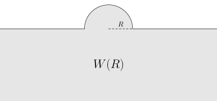
Figure 1.1. The region $W(R)$.

Corollary 1.15.

Let $B(a,1)\subset\mathbb{R}^{2n}$ be the (open) ball of radius $1$ centered at $a=(0,\dots,0,-|a|)$, let $r$ satisfy $|a|^{2}+r^{2}=1$ (so that, in particular, $B^{n,k}(r)=B(a,1)\cap\mathbb{R}^{n,k}$), and suppose that $k<n$.

There exists a relative symplectic embedding

$$\phi\colon(B(a,1),B^{n,k}(r),\omega_{0})\hookrightarrow(W(R),W^{n,k}(R),\omega_{0}),$$

such that any two distinct isotropic leaves of $B^{n,k}(r)$ are mapped to distinct leaves of $W^{n,k}(R)$ if and only if

$$\arcsin(r)-r(1-r^{2})^{1/2}\leq\frac{\pi}{2}R^{2}.$$

Remark 1.16.

The significance of this lower bound becomes clear in the 2-dimensional case. Consider the disk $B(a,1)\subset\mathbb{R}^{2}$ of radius $1$ centered at $a$, then $B^{1,0}(r)$ is (the interior of) a chord of the circle $\partial B(a,1)$. This chord cuts the disk into two regions.

The quantity

$$\arcsin(r)-r(1-r^{2})^{1/2}$$

is the area of the smaller of the two regions.

In this two dimensional case, $W(R)$ is precisely the region shown in Figure 1.1, and $\mathbb{R}^{1,0}=\mathbb{R}$ cuts the region into the lower half-plane and an open half-disk of radius $R$. This half-disk has area $\pi R^{2}/2$. This obstruction is therefore obvious in dimension 2.

Thus, the content of this corollary is that this a priori two dimensional area obstruction continues to hold in higher dimensions. The dynamical origins of the left side of the inequality may be observed in Proposition 2.7 and its proof.

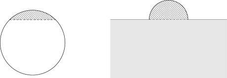
Figure 1.2. The 2-dimensional case. The hashed area on the left must be less than the hashed area on the right for the embedding to exist.

Observe that $\mathbb{R}^{2n-2}\times W(1)$ has infinite Gromov width, so this embedding is only obstructed by the coisotropic constraint.

Several additional applications also follow given the existence of the coisotropic capacity $c$, again using techniques from [Hofer_Zehnder_1994]. We give a few of these applications to the existence of chords in Section 4. In particular, we have: thmThmAlmostExistence

Let $(M,\omega)$ be a symplectic manifold. Let $S\hookrightarrow M$ be a compact, regular energy surface for the Hamiltonian $H$. Without loss of generality, $S=H^{-1}(1)$. Let $N\hookrightarrow M$ be an $(n+k)$-dimensional coisotropic submanifold transverse to $S$, and let $\sim$ be the leafwise relation on $N$.

Suppose there is a neighbourhood $U$ of $S$ such that ${c}(U,N,\omega,\sim)<\infty$.

Then there is a $\rho>0$ and a dense subset $\Sigma\subset[1-\rho,1+\rho]$ such that $X_{H}$ admits a leafwise chord on every energy surface of $H$ with energy in $\Sigma$.

2. Capacities relative to coisotropic submanifolds

We now begin the proof of Theorem 1.14, giving the monotonicity and conformality axioms, as well as a lower bound. We follow the construction of the Hofer-Zehnder capacity from [Hofer_Zehnder_1994]. We also provide a proof of Corollary 1.15.

Let $(M,N)$ be a pair consisting of a symplectic manifold $(M,\omega)$ and a properly embedded coisotropic submanifold $N\hookrightarrow M$, i.e. with $\partial N\subset\partial M$ (or $\partial N=\emptyset$). All of our symplectic manifolds will be assumed to be of the same dimension $2n$.

We begin with a few definitions.

Definition 2.1.

Recall that

$$\mathbb{R}^{n,k}\coloneqq\{x\in\mathbb{R}^{2n}|x=(x_{1},\dots,x_{n},y_{1},\dots,y_{k},0,\dots,0)\}$$

is an $(n+k)$-dimensional coisotropic linear subspace of $\mathbb{R}^{2n}$, and that $B(a,r)$ is the $2n$ dimensional symplectic ball of radius $r$ centered at

$$a\coloneqq(0,\dots,0,b_{n})\in\mathbb{R}^{2n},$$

and $B^{n,k}(r)\subset\mathbb{R}^{n,k}$ as the coisotropic ball of radius $r$ centered at $0\in\mathbb{R}^{n,k}$:

$$B^{n,k}(r)\coloneqq\{x\in\mathbb{R}^{n,k}\,|\,|x|\,\leq r\}.$$

Figure 2.1. A schematic image of the embedding of $B^{n,k}(r)$ into $B(a,1)$.

Recall that we likewise denote by

$$Z(a,r)\coloneqq\{x\in\mathbb{R}^{2n}\,|\,x_{n}^{2}+(y_{n}-b_{n})^{2}\leq r^{2}\}$$

the symplectic cylinder centered at $a\in\mathbb{R}^{2n}$, and by $Z^{n,k}(r)$ the coisotropic cylinder

$$Z^{n,k}(r)\coloneqq\{x\in\mathbb{R}^{n,k}\,|\,|x_{n}|\leq r\}$$

Remark 2.2.

Note that $B^{n,k}(r)$ and $Z^{n,k}(r)$ are properly embedded in $B(a,1)$, $Z(a,1)$, respectively, when $a=(0,\dots,0,b_{n})$ with $|b_{n}|<1$, and $r^{2}=1-|a|^{2}$. See Figure 2.1.

We will now study the properties of the map $c(M,N,\omega,\sim)$. We will show that this satisfies the axioms for coisotropic capacities.

We prove the monotonicity and conformality properties below, which proceed as in [Hofer_Zehnder_1994]. The proof of non-triviality will be completed in Section 3.

Lemma 2.3.

The map $c$ satisfies the monotonicity axiom.

Proof.

Let $\phi\colon(M_{1},N_{1},\omega_{1},\sim_{1})\to(M_{2},N_{2},\omega_{2},\sim_{2})$ be a relative embedding, respecting the coisotropic equivalence relations, as in Definition 1.5. Define the map $\phi_{*}\colon\mathcal{H}(M_{1},N_{1})\to\mathcal{H}(M_{2},N_{2})$ by

$$\phi_{*}(H)=\begin{cases}H\circ\phi^{-1}&x\in\phi(M_{1})\\ m(H)&x\notin\phi(M_{1})\end{cases}$$

Note that if $A\subset M_{1}\setminus\partial M_{1}$ is a non-empty compact set and $\emptyset\subsetneq A\cap N_{1}\subsetneq N_{1}$, then $\phi(A)\subset M_{2}\backslash\partial M_{2}$ and $\emptyset\subsetneq\phi(A)\cap N_{2}\subsetneq N_{2}$. By construction, $m(H)=m(\phi_{*}(H))$. If $U\subset M_{1}$ is an open set on which $H=0$, then, since $\phi$ is an embedding $\phi(U)$ is an open set on which $\phi_{*}(H)=0$. Also, by construction, $0\leq\phi_{*}(H)\leq m(\phi_{*}(H))$, and therefore $\phi_{*}(H)\in\mathcal{H}(M_{2},N_{2},\omega_{2})$.

We now check that $\phi_{*}(\mathcal{H}_{a}(M_{1},N_{1},\omega_{1},\sim_{1}))\subset\mathcal{H}_{a}(M_{2},N_{2},\omega_{2},\sim_{2})$. Let $H\colon M_{1}\to\mathbb{R}$ be an admissible simple Hamiltonian. Since $\phi$ is symplectic, $\phi_{*}(X_{H})=X_{\phi_{*}(H)}$. Furthermore, the Hamiltonian vector field $X_{\phi_{*}(H)}$ vanishes outside the image of $\phi$. Thus, all non-constant trajectories of $X_{\phi_{*}(H)}$ are conjugate to non-constant trajectories of $X_{H}$. In particular then, if $y(t)$ is a non-constant trajectory of $X_{\phi_{*}(H)}$ with $y(0)\in N_{2},y(T)\in N_{2}$ with $y(0)\sim_{2}y(T)$, then $y(t)$ must be in the image of $\phi$ and thus there exists a trajectory $x(t)$ of $X_{H}$ so that $\phi(x(t))=y(t)$.

Since $\phi$ is a relative embedding with $\phi^{-1}(N_{2})=N_{1}$, we have that $x(0),x(T)\in N_{1}$. Since the relative embedding $\phi$ respects the coisotropic equivalence relations, if $y(0)\sim_{2}y(T)$ then it must hold that $x(0)\sim_{1}x(T)$. As $H\in\mathcal{H}_{a}(M_{1},N_{1},\omega_{1},\sim_{1})$, it follows that $T>1$. Hence, it follows that $\phi_{*}H\in\mathcal{H}_{a}(M_{2},N_{2},\omega_{2},\sim_{2})$, as desired.

∎

We now give a slight extension of the above monotonicity, which will be of use to us in the proof of Theorem 3.26.

Lemma 2.4.

Let $(M,\omega)$ and $(M^{\prime},\omega^{\prime})$ be symplectic manifolds, let $N\subset M$ and $N^{\prime}\subset M^{\prime}$ be coisotropic submanifolds equipped with coisotropic equivalence relations $\sim$ and $\sim^{\prime}$.

Suppose that for every compact set $K\subset M$, there exists an open neighbourhood $U\supset K$ and a relative symplectic embedding $\psi\colon(U,N\cap U,\omega|_{U})\to(M,N,\omega)$ that respects the pair of coisotropic equivalence relations $(\sim,\sim^{\prime})$.

Then, $c(M,N,\omega,\sim)\leq c(M^{\prime},N^{\prime},\omega^{\prime},\sim^{\prime})$.

Proof.

Let $H\colon M\to\mathbb{R}$ be a Hamiltonian with $0\leq H\leq m(H)$ and that $m(H)-H$ is compactly supported in $M$. Then, by hypothesis, there exists a neighbourhood $U$ of the support of $m(H)-H$ and a symplectic embedding $\psi\colon U\to M^{\prime}$. Let $G=H\circ\psi^{-1}$ defined on $\psi(U)$ and then extend $G$ to all of $M^{\prime}$ by setting $G(x)=m(H)$ for all $x\notin\psi(U)$.

Proceeding as in Lemma 2.3, it follows that $G$ is simple if and only if $H$ is simple, with $m(G)=m(H)$. Furthermore, $X_{G}=\psi_{*}X_{H}$ on $\psi(U)$ and vanishes outside $\psi(U)$. Thus, arguing as in Lemma 2.3, $G$ is admissible if and only if $H$ is.

Thus for any $H\in\mathcal{H}_{a}(M,N,\omega,\sim)$, there exists $G\in\mathcal{H}_{a}(M^{\prime},N^{\prime},\omega^{\prime},\sim^{\prime})$ such that $m(H)=m(G)$. The desired inequality now follows immediately. ∎

Remark 2.5.

The monotonicity of the capacity depends in an essential way on the coisotropic equivalence relation. Indeed, if no condition is put on the relative embedding $\phi\colon(M_{1},N_{1},\omega_{1})\to(M_{2},N_{2},\omega_{2})$, it is easy to imagine a situation in which two or more leaves on $N_{1}$ are mapped to the same leaf in $N_{2}$. For instance, there are many examples of compact hypersurfaces in $\mathbb{R}^{2n}$ for which there is a dense leaf in the characteristic foliation — in this case, this is about dense orbits in a Hamiltonian system with compact energy level. One possible construction is originally due to Katok [Katok_1973], as is used in [Casals_Spacil_2016]. In particular, Katok’s construction can be done as a small, locally supported perturbation of the unit sphere in $\mathbb{R}^{2n}$. This construction of Katok’s also shows that the existence of leafwise chords must see the entirety of the coisotropic submanifold.

As discussed in Example 1.6, a natural class to consider is to consider a fixed (compact) coisotropic submanifold $\hat{N}$ in $\mathbb{R}^{2n}$. We then consider only symplectic manifolds that are open subsets $U\subset\mathbb{R}^{2n}$ and coisotropic submanifolds $N=\hat{N}\cap U$. The coisotropic equivalence relation is that $x\sim y$ if and only if $x,y$ are in the same isotropic leaf on $\hat{N}$. Then, all of the inclusion maps respect the equivalence relation, by construction.

A very simple example of this phenomenon occurs even with Lagrangians. Let $(\hat{M},\hat{N})$ be the pair consisting of the unit disk in $\mathbb{R}^{2}$ and the $x$-axis. Let $M$ be an open annulus centred at the origin. Then, $N=\hat{N}\cap M$ is the disjoint union of two line segments.

In $M$, each line segment is its own leaf: an admissible Hamiltonian for the leafwise relation, just considered relative to $N$, would allow for a finger move that pushed centre of the segments almost all the way around the annulus.

Notice however that the inclusion of $(M,N)\hookrightarrow(\hat{M},\hat{N})$ does not respect the leafwise relation! The two leaves of $\hat{N}$ are both mapped to the unique leaf of $N$. Relative to the equivalence relation induced from the leafwise relation on $\hat{N}$, however, these chords from one segment to the other would be eliminated.

We thank Kaoru Ono and Yoshihiro Sugimoto for pointing out that our original version of this capacity $c$ overlooked this point and implicitly required the embeddings to respect the leaf relation.

Lemma 2.6.

$c$ satisfies the conformality axiom.

Proof.

Let $\alpha\neq 0$. Define a map $\psi\colon\mathcal{H}(M,N)\to\mathcal{H}(M,N)$ by

$$\psi(H)\coloneqq|\alpha|\cdot H,$$

and let $H_{\alpha}$ denote $\psi(H)$.

Note that $\psi$ is clearly injective, and $m(H_{\alpha})=|\alpha|m(H)$, so the lemma follows if

$$\psi|_{\mathcal{H}_{a}(M,N,\omega,\sim)}\colon\mathcal{H}_{a}(M,N,\omega,\sim)\to\mathcal{H}_{a}(M,N,\alpha\omega,\sim)$$

is a bijection. Let $X_{H_{\alpha}}$ be the Hamiltonian vector field generated by $H_{\alpha}$ with respect to $\alpha\omega$, in other words such that $\alpha\omega(X_{H_{\alpha}},\cdot)=-dH_{\alpha}$. Hence,

$$\alpha\omega(X_{H_{\alpha}},\cdot)=-|\alpha|dH \omega(X_{H_{\alpha}},\cdot)=-\frac{|\alpha|}{\alpha}dH.$$

Thus, $X_{H_{\alpha}}=\pm X_{H}$, depending on the sign of $\alpha$. Therefore, the Hamiltonian flows for $H$ and $H_{\alpha}$ have the same orbits. In particular, the constant chords are the same for the two Hamiltonians. A non-constant chord for one of them, $x(0)\in N$, $x(T)\in N$ with $x(0)\sim x(T)$, will be a chord for the other, by considering $x(t)$ itself if $\alpha>0$ and the time reversal $t\mapsto x(T-t)$ if $\alpha<0$. Their return times are thus the same. ∎

In the next proposition, we give a lower bound for $c\left(B(a,1),B^{n,k}(r),\omega_{0}\right)$ with $r=\sqrt{1-|a|^{2}}$.

Proposition 2.7.

Let $a\coloneqq(0,\dots,0,b)\in\mathbb{R}^{2n}$, and set $r^{2}=1-|a|^{2}=1-|b|^{2}$. For $k\in\{0,\dots,n-1\}$,

$$c\left(B(a,1),B^{n,k}(r),\omega_{0}\right)\geq\arcsin(r)-r(1-r^{2})^{1/2}.$$

Proof.

We consider first when $|a|>0$. We suppose, without loss of generality, that $b<0$ and thus $b=-|a|$.

We will construct a family of Hamiltonian functions all of which are admissible and whose maximum is arbitrarily close to $\arcsin(r)-r(1-r^{2})^{1/2}$. First, decompose $\mathbb{R}^{2n}=\mathbb{R}^{n}\oplus J\mathbb{R}^{n}=(x_{1},\dots,x_{n},y_{1},\dots,y_{n})$, where $J:\mathbb{R}^{2n}\to\mathbb{R}^{2n}$

(2.1) $$\begin{split}J(0,\dots,0,x_{i},0,\dots,0)&=(0,\dots,0,y_{i},0,\dots,0)\\ J(0,\dots,0,y_{i},0,\dots,0)&=(0,\dots,0,-x_{i},0,\dots,0),\end{split}$$

and we understand $J\mathbb{R}^{n}$ to indicate $J$ applied to the first $n$ dimensions of $\mathbb{R}^{2n}$. Choose $\epsilon>0$, and let $f\colon[0,1]\subset\mathbb{R}\to\mathbb{R}$ be a function with the following properties:

$$f(t)=0 \text{ for }t\in[0,|a|+\epsilon],$$

$$0\leq f^{\prime}(t)<\arccos\left(\frac{|a|}{\sqrt{t}}\right)\quad \text{ for }t>|a|+\epsilon,$$

$$f(t)=\max f\quad \text{ for }t\in[1-\epsilon,1].$$

Let $H\colon\mathbb{R}^{2n}\to\mathbb{R}$ be the Hamiltonian defined by $H(x)\coloneqq f(|x-a|^{2})$.

We will first observe that $H$ is simple. Note first of all that $H=0$ in an open ball around $a$, and this ball intersects $B^{n,k}(r)$, as required. Also observe that $H=\max f$ once $|x-a|^{2}\geq 1-\epsilon$, so this gives $H=\max f$ in a collar neighbourhood of the boundary of $B(a,1)$ as required.

We will now show that any such Hamiltonian $H$ will be admissible.

We consider the associated Hamiltonian ODE given by

$$\dot{x}=J\nabla H(x)= 2f^{\prime}\left(|x-a|^{2}\right)J(x-a)$$

where $J\colon\mathbb{R}^{2n}\to\mathbb{R}^{2n}$ is the standard almost complex structure defined by Equation 2.1 above. Since $\langle Jx,x\rangle=0$, we see that $|x-a|^{2}$ is constant along solutions of the equation. Thus, with $z(t)\coloneqq x(t)-a$ we have for $\kappa=2f^{\prime}(|z(0)|^{2})\geq 0$,

(2.2) $$\dot{z}=\kappa Jz.$$

Thus, $z(t)=\operatorname{e}^{\kappa Jt}z(0)$.

If a trajectory $z(t)$ starts on the coisotropic submanifold, we then have the initial conditions

$$z(0)\in\mathbb{R}^{n,k}.$$

To verify admissibility, we will show that every non-constant trajectory starting on the coisotropic submanifold has (non-leafwise, coisotropic) return time greater than $1$.

Let $z(t)$ be such a non-constant trajectory, with $z(0)\in B^{n,k}(r)$. It follows then that $\kappa\neq 0$. Now consider the triangle formed by the origin, $a$, and $c=(0,\dots,-r,0,\dots,0)$, where the $-r$ is in the $n$-th position. Note that, if we consider the plane defined by these three points, then any flow $z(t)$ with $z(0)$ on the line from $a$ to $c$ flows counterclockwise in this plane. Since $f$ is a radial function, we may, without loss of generality, simply consider any such flow $z(t)$ with $z(0)$ on this line.

Figure 2.2.

Let $\rho=\sqrt{|x(0)|^{2}+|a|^{2}}=|z(0)|\geq|a|$, and let $\theta$ be the angle so that $|x(0)|=\rho\cos(\theta)$ and $|a|=\rho\sin(\theta)$. See Figure 2.2 for an illustration. Hence, $\theta=\arcsin(\frac{|a|}{\rho})$. If $T$ is such that $z(T)$ belongs to $\mathbb{R}^{n,k}$, we have $\sin(\kappa T+\theta)=\sin(\theta)=\frac{|a|}{\rho_{z}}$, which holds if and only if $\kappa T\in 2\pi\mathbb{Z}$ or $\kappa T=-2\theta+k\pi$ for some $k$ odd. In particular then, if $\kappa<\pi-2\theta$, there can be no chords of length at most $1$. Recall now that $\kappa=2f^{\prime}(|z(0)|^{2})$. Thus, the condition is satisfied if we have $2f^{\prime}(\rho^{2})<\pi-2\theta$ for each $\rho_{z}$. This is achieved if

$$f^{\prime}(\rho^{2})<\frac{\pi}{2}-\theta=\arccos\left(\frac{|a|}{\rho}\right)$$

However, by assumption, $f^{\prime}(\rho_{z}^{2})<\arccos\left(\frac{|a|}{\rho_{z}}\right)$. Observe now that by choosing $\epsilon>0$ sufficiently small, we may arrange for $f(1)$ to be arbitrarily close to

$$\int_{|a|^{2}}^{1}\arccos\left(\frac{|a|}{\sqrt{t}}\right)dt =\int_{0}^{\arccos(|a|)}2|a|^{2}\alpha\cos(\alpha)^{-3}\sin(\alpha)d\alpha$$

$$=|a|^{2}\left(\alpha\cos(\alpha)^{-2}-\tan\alpha\right)\Big{|}_{0}^{\arccos(|a|)}$$

$$=\arcsin r-r\sqrt{1-r^{2}}.$$

(Recalling that $a^{2}+r^{2}=1$.)

From this, we conclude

$$c(B(a,1),B^{n,k}(r),\omega_{0})\geq\arcsin(r)-r(1-r^{2})^{1/2},$$

as desired, in the case that $|a|>0$.

If $a=0$, we observe that for each $\delta>0$, we may set $p=(0,\dots,0,-\delta)$ and then we consider the inclusion of the ball $B(p,1-\delta)\subset B(0,1)$. The intersection of $B^{n,k}(r)$ with this smaller ball is given by $B^{n,k}(\sqrt{1-2\delta})+p$. After a translation of the origin, this gives a relative embedding of the pair $(B(-p,1-\delta),B^{n,k}(\sqrt{1-2\delta}))$. Let $r_{\delta}=\sqrt{1-2\delta}$. Then, applying the above construction and the Monotonicity Axiom (Lemma 2.3), we have for each $\delta>0$,

$$c(B(0,1),B^{n,k}(1),\omega_{0})\geq\arcsin(r_{\delta})-r_{\delta}(1-r_{\delta}^{2})^{1/2}$$

Taking $\delta\to 0$, we obtain $c(B(0,1),B^{n,k}(1))\geq\arcsin(1)=\frac{\pi}{2}$, proving the result.

∎

Proof of Corollary 1.15.

By the non-triviality and conformality axioms for the capacity, we obtain that $c(W(R),W^{n,k}(R))=\frac{\pi}{2}R^{2}$.

The monotonicity of the capacity $c$ and Proposition 2.7 then give that a relative embedding $(B(a,1),B^{n,k}(r))\hookrightarrow(W(R),W^{n,k}(R))$ respecting the leaf relations exists only if

$$\arcsin(r)-r(1-r^{2})^{1/2}\leq\frac{\pi}{2}R^{2}.$$

To prove that this suffices, we will construct an embedding for any $R$ that satisfies

$$\arcsin(r)-r(1-r^{2})^{1/2}<\frac{\pi}{2}R^{2}.$$

By a slight abuse of notation (since $a\in\mathbb{R}^{2n}$), let $D(a,\rho)\subset\mathbb{R}^{2}$ be the disk of radius $\rho$ centred at $(0,-|a|)$.

First, we notice that the ball embeds in an appropriate polydisk:

$$B(a,1)\subset D^{2}(0,1)\times\dots D^{2}(0,1)\times D^{2}(a,1)$$

$$\begin{split}=&\{(x_{1},\dots,x_{n},y_{1},\dots,y_{n})\,|\\ &\quad x_{1}^{2}+y_{1}^{2}<1,\dots,x_{n-1}^{2}+y_{n-1}^{2}<1,(x_{n}+a)^{2}+y_{n}^{2}<1\}.\end{split}$$

This respects the leaf relation on $\mathbb{R}^{n,k}$.

We will now construct an embedding

$$\psi\colon D^{2}(0,1)\times\dots D^{2}(0,1)\times D^{2}(a,1)\to W(R)$$

of the form

$$\psi(x_{1},\dots,x_{n-1},x_{n},y_{1},\dots,y_{n-1},y_{n})=(x_{1},\dots,x_{n-1},f(x_{n},y_{n}),y_{1},\dots,y_{n-1},g(x_{n},y_{n}))$$

for a suitable choice of map

$$\phi\colon\mathbb{R}^{2}\to\mathbb{R}^{2},\phi(x,y)=(f(x,y),g(x,y)).$$

Let $W^{2}(R)\coloneqq\{(x,y)\in\mathbb{R}^{2}\,|\,x^{2}+y^{2}<R^{2}\text{ or }y<0\}$. Observe now that $\psi$ is symplectic if and only if $\phi$ is area preserving. Furthermore, $\psi$ gives a relative embedding of the polydisk into $W(R)$ (with coisotropic submanifold given by the restriction of $\mathbb{R}^{n,k}$ to each) if and only $\phi\colon(D(a,1),\mathbb{R}\cap D(a,1))\to(W^{2}(R),\mathbb{R}\cap W^{2}(R))$ is a relative embedding. Finally, we observe that if $\phi$ is such a relative embedding, it immediately follows from the explicit description of the leaf relation in Example 1.3 that $\psi$ respects the leaf relation.

It suffices therefore to find an embedding $\phi\colon D(a,1)\to W^{2}(R)$. By a standard Moser-type argument, this exists whenever the area of the smaller of the two connected components of $D^{2}(a,1)\setminus\mathbb{R}$ is strictly smaller than the area of the upper half disk in $W^{2}(R)\setminus\mathbb{R}$. The result now follows by computing this area, as in Remark 1.16.

∎

3. An upper bound for $c\left(U(r),U^{n,k}(r),\omega_{0},\sim\right)$

In the following, we will write $c(M,N)=c(M,N,\omega,\sim)$ since we are considering subsets $M\subset\mathbb{R}^{2n}$ with respect to the standard symplectic form. Furthermore, we will take the equivalence relation to be the leafwise equivalence relation.

In order to show that $c$ is a coisotropic capacity, we must establish the non-triviality axiom. Recall that we have defined

$$W(1)=\left\{(x_{1},\dots,x_{n},y_{1},\dots,y_{n})\in\mathbb{R}^{2n}\;|\;x_{n}^{2}+y_{n}^{2}<1\text{ or }y_{n}<0\right\}$$

and $W^{n,k}(1)=W(1)\cap\mathbb{R}^{n,k}$, with $\mathbb{R}^{n,k}$ the standard $(n+k)$-dimensional coisotropic subspace of $\mathbb{R}^{2n}$, given by

$$\mathbb{R}^{n,k}=\left\{(x_{1},\dots,x_{n},y_{1},\dots,y_{k},0,\dots,0)\right\}.$$

By the relative symplectic embedding of the ball

$$(B(1),B^{n,k}(1))\hookrightarrow(W(1),W^{n,k}(1)),$$

and monotonicity (Lemma 2.3), together with Proposition 2.7, it suffices to prove the following inequality:

$$c(W(1),W^{n,k}(1))\leq\frac{\pi}{2}.$$

For our analytical set-up, it is most convenient to work with the region $U(1)$ in $\mathbb{R}^{2n}$ given as the union of the disk with a half-infinite strip

$$U(1)=\mathbb{R}^{2n-2}\times\{(x,y)\in\mathbb{R}^{2}\,|\,x^{2}+y^{2}<1\text{ or }-1<x<1\text{ and }y<0\}$$

and $U^{n,k}(1)=U(1)\cap\mathbb{R}^{n,k}$. In the following, we will write $U=U(1)$ and $U^{n,k}=U^{n,k}(1)$.

We claim that the relative capacities of these two domains are the same:

$$c(W(1),W^{n,k}(1))=c((U(1),U^{n,k}(1))).$$

Observe that there is a relative embedding

$$(U(1),U^{n,k}(1))\hookrightarrow(W(1),W^{n,k}(1))$$

by inclusion, showing one inequality. The other inequality is by applying Lemma 2.4. Indeed, for any compact set $K\subset W(1)$, by a Moser argument, we may find an open neighbourhood $V$ and a symplectic embedding $V\hookrightarrow U(1)$ that may be taken to the the identity in the region $y_{n}>-\delta$ for $\delta>0$ sufficiently small, and hence is the identity on the coisotropic submanifold. The existence of such a symplectic embedding for each compact $K\subset W(1)$ then verifies the hypotheses of the Lemma, and the claim follows.

Proposition 3.1.

The map $c$ verifies

$$c(U,U^{n,k})\leq\frac{\pi}{2}.$$

As explained above, this will then prove Theorem 1.14. The remainder of this section will prove Proposition 3.1.

3.1. The analytical setting

Definition 3.2.

We recall from Example 1.3 that $\omega_{0}$ denotes the standard symplectic form on $\mathbb{R}^{2n}$, and that $\mathbb{R}^{n,k}$ is the linear coisotropic subspace of $(\mathbb{R}^{2n},\omega_{0})$ consisting of the first $n+k$ coordinates, i.e.

$$\mathbb{R}^{n,k}=\left\{x\in\mathbb{R}^{2n}\;|\;x=(x_{1},\dots,x_{n},y_{1},\dots,y_{k},0,\dots,0)\right\}.$$

Let $V_{0},V_{1}$ and $W_{0}$ be the linear subspaces

$$V_{0} =\left\{x\in\mathbb{R}^{2n}\;|\;x=(0,\dots,0,x_{k+1},\dots,x_{n},0,\dots,0)\right\},$$

$$V_{1} =\left\{x\in\mathbb{R}^{2n}\;|\;x=(x_{1},\dots,x_{k},0,\dots,0,y_{1},\dots,y_{k},0\cdots,0)\right\}$$

$$W_{0} =\left\{\in\mathbb{R}^{2n}\;|\;x=(0,\dots,0,y_{k+1},\dots,y_{n})\right\}.$$

Remark 3.3.

As noted in Example 1.3, any leaf $F$ in the characteristic foliation has the form $z+V_{0}$, for $z\in\mathbb{R}^{n,k}$.

Let $C_{n,k}^{\infty}\left([0,1]\right)$ denote the space of smooth maps $\psi:[0,1]\to\mathbb{R}^{2n}$ such that $\psi(0),\psi(1)\in F\subset\mathcal{F}$ for some isotropic leaf $F$ in the characteristic foliation $\mathcal{F}$ of $\mathbb{R}^{n,k}$. Let $\langle\cdot,\cdot\rangle$ be the standard inner product on $\mathbb{R}^{2n}$, and define the functional $\Phi_{H}\colon C_{n,k}^{\infty}\left([0,1]\right)\to\mathbb{R}$ by

(3.1) $$\Phi_{H}(\psi)=\frac{1}{2}\int_{0}^{1}\langle-J\dot{\psi}(t),\psi(t)\rangle dt-\int_{0}^{1}H(\psi(t))dt.$$

In order to study the critical points of $\Phi_{H}$, we will extend the definition of $\Phi_{H}$ to the Hilbert space of $H^{1/2}$ paths. The Hilbert space is constructed so the paths have boundary in $\mathbb{R}^{n,k}$, even though $H^{1/2}$ does not embed in $C^{0}$, and thus a pointwise constraint cannot be imposed. The key observation we use is that $\mathbb{R}^{n,k}$ is the fixed point locus of an involution on $\mathbb{R}^{2n}$, which then induces an isometry on $H^{1/2}(S^{1},\mathbb{R}^{2n})$. Our path space is then an eigenspace of this isometry, though we also describe it explicitly.

We first show the following.

Lemma 3.4.

Any element $\gamma\in C^{\infty}_{n,k}\left([0,1]\right)$ is given by

(3.2) $$\gamma(t)=\sum_{k\in\mathbb{Z}}e^{k\pi Jt}a_{k}+\sum_{k\in 2\mathbb{Z}}e^{k\pi Jt}b_{k}$$

where

(3.3) $$\begin{split}&a_{k}\in V_{0}\subset\mathbb{R}^{n,k}\subset\mathbb{R}^{2n},\text{ and }\\ &b_{k}\in V_{1}\subset\mathbb{R}^{n,k}\subset\mathbb{R}^{2n}.\end{split}$$

Equivalently,

$$\gamma(t)=\sum_{k\in\mathbb{Z}}z_{k}e^{k\pi Jt}$$

with $z_{k}\in V_{0}$ for odd $k$ and $z_{k}\in V_{0}\oplus V_{1}$ for even $k$ (i.e. $z_{k}=a_{k}+b_{k}$ with $b_{k}=0$ for all odd $k$).

Proof.

We begin by identifying $\mathbb{R}^{2}$ with $\mathbb{C}$, and we consider a smooth map $\gamma(t):[0,1]\to\mathbb{C}$ such that $\gamma(0),\gamma(1)\in\mathbb{R}\subset\mathbb{C}$. We now extend this map to a piecewise smooth map $\alpha(t):S^{1}\to\mathbb{C}$ by

$$\alpha(t)=\begin{cases}\gamma(2t)&t\in\left[0,\frac{1}{2}\right]\\ \overline{\gamma(2-2t)}&t\in\left(\frac{1}{2},1\right],\end{cases}$$

where the bar indicates complex conjugation. Note that $\alpha(t)$ is continuous by definition. Writing $\alpha(t)$ in terms of its Fourier decomposition, we have

$$\alpha(t)=\sum_{k}e^{2\pi ikt}a_{k}.$$

However, since $\alpha(t)=\overline{\alpha(1-t)}$, and therefore

$$\sum_{k}e^{2\pi ikt}a_{k} =\sum_{k}e^{-2\pi ik(1-t)}\overline{a_{k}}$$

$$=\sum_{k}e^{-2\pi ik}e^{2\pi ikt}\overline{a_{k}}$$

$$=\sum_{k}e^{2\pi ikt}\overline{a_{k}},$$

which implies that $a_{k}=\overline{a_{k}}$, and therefore $a_{k}\in\mathbb{R}\subset\mathbb{C}$. Our original function $\gamma(t)$ is recovered by $\gamma(t)=\alpha(t/2)=\sum_{k}e^{\pi ikt}a_{k}$, where $a_{k}\in\mathbb{R}$.

Now consider a function $\gamma(t):[0,1]\to\mathbb{R}^{2n}$ such that $\gamma(0),\gamma(1)\in F$, where $F$ is a leaf of the characteristic foliation of $\mathbb{R}^{n,k}$. Write a point $x\in\mathbb{R}^{2n}$ by $(x_{1},\dots,x_{n},y_{1},\dots,y_{n})$, where $\omega_{0}(\frac{\partial}{\partial x_{i}},\frac{\partial}{\partial y_{i}})=1$, $J\frac{\partial}{\partial x_{i}}=\frac{\partial}{\partial y_{i}}$, for $J$ the standard complex structure on $\mathbb{R}^{2n}$, and define $c_{n,k}:\mathbb{R}^{2n}\to\mathbb{R}^{2n}$ by

$$c_{n,k}(x):=(x_{1},\dots,x_{n},y_{1},\dots,y_{k},-y_{k+1},-y_{n}).$$

Recall that $\mathbb{R}^{n,k}$ is the set of points

$$\mathbb{R}^{n,k}=\{x\in\mathbb{R}^{2n}|x=(x_{1},\dots,x_{n},y_{1},\dots,y_{k},0,\dots,0)\}.$$

In the special case of a Lagrangian, i.e. for $\mathbb{R}^{n,0}$, we note that $c_{n,0}$ is a real structure for $\omega_{0}$, i.e. $c_{n,0}^{*}\omega_{0}=-\omega_{0}$.

Any leaf $F$ of $\mathcal{F}$ is a set of the form

$$\{x\in\mathbb{R}^{n,k}\,|\,x=(0,\dots,0,x_{k+1},\dots,x_{n},0,\dots,0)+z\}$$

for some fixed $z=(x_{1},\dots,x_{k},0,\dots,0,y_{1},\dots,y_{k},0,\dots,0)$. We may write $\gamma(t)$ as a function $\gamma(t)=z_{1}(t)+z_{2}(t)+\dots+z_{n}(t)$, where each function $z_{i}\colon[0,1]\to\mathbb{R}^{2n}$ is a map $t\mapsto(0,\dots,0,x_{i}(t),0,\dots,0,y_{i}(t),0,\dots,0)$ for real functions $x_{i},y_{i}:[0,1]\to\mathbb{R}$.

From the above, we see that if $i>k$, then

$$z_{i}(t)=\sum_{j}e^{J\pi jt}a_{i,j}$$

where $a_{i,j}=a_{j}e_{i}$ for constants $a_{j}\in\mathbb{R}$, $e_{i}$ a vector with $1$ in the $i$-th position and $0$s elsewhere. This then gives that $a_{i,j}\in V_{0}$.

For $i\leq k$, $z_{i}(0)=z_{i}(1)$, and we have

$$z_{i}(t)=\sum_{j}e^{2\pi jJt}a_{i,j},$$

where $a_{i,j}=a_{j}e_{i}$ with $a_{j}\in\mathbb{C}$. From this, we have that $a_{i,j}\in V_{1}$.

The conclusion of the lemma now follows immediately. ∎

Remark 3.5.

Note that if $\gamma\in C^{0}([0,1],\mathbb{R}^{2n})\cap L^{1}$ and is of the form

$$\gamma(t)=\sum_{k\in\mathbb{Z}}e^{k\pi Jt}a_{k}+\sum_{k\in 2\mathbb{Z}}e^{k\pi Jt}b_{k}$$

with $a_{k},b_{k}$ as in Equation 3.3 above, then necessarily $\gamma(0),\gamma(1)\in F$.

Definition 3.6.

Let $L^{2}_{n,k}([0,1])$ be the Hilbert space

$$\begin{split}L^{2}_{n,k}=\bigg{\{}\gamma\in L^{2}([0,1],\mathbb{R}^{2n})\,\bigg{|}\,&\gamma=\sum_{k\in\mathbb{Z}}a_{k}e^{k\pi Jt}+\sum_{k\in 2\mathbb{Z}}b_{k}e^{k\pi Jt},\\ &\,a_{k}\in V_{0},\,b_{k}\in V_{1},\\ &\sum_{k\in\mathbb{Z}}|a_{k}|^{2}+|b_{k}|^{2}<\infty\bigg{\}}\end{split}$$

with inner product

$$\left\langle\psi,\phi\right\rangle_{L^{2}_{n,k}}=\left(\int_{0}^{1}\langle\psi(t),\phi(t)\rangle\,dt\right)^{\frac{1}{2}}.$$

Define $H_{n,k}^{s}\left([0,1]\right)$ to be the space

$$H_{n,k}^{s}([0,1])=\left\{x\in L^{2}_{n,k}\left([0,1]\right)\>\bigg{|}\;\sum_{k\in\mathbb{Z}}|k|^{2s}|z_{k}|^{2}<\infty\right\}$$

where $z_{k}\in V_{0}$ for odd $k$ and $z_{k}\in V_{0}\oplus V_{1}$ for even $k$.

In the following lemmas, we collect several standard results from [Hofer_Zehnder_1994] concerning the spaces $H^{s}_{n,k}([0,1])$. The proofs are identical to those in [Hofer_Zehnder_1994], replacing the spaces considered there with the corresponding spaces in our setting. For the convenience of the reader, we have tried to keep our notation compatible with the notation of [Hofer_Zehnder_1994]*Sections 3.3, 3.4. One notable change is that we use $X$ to denote the appropriate $H^{\frac{1}{2}}$ Hilbert space, which is denoted by $E$ in [Hofer_Zehnder_1994]. Some of the more immediate results are stated without proof.

Definition 3.7.

Denote by

$$X=H^{1/2}_{n,k}\left([0,1]\right).$$

For $\gamma\in X$, we have

$$\gamma=\sum_{k\in\mathbb{Z}}z_{k}e^{k\pi Jt}$$

where $z_{k}\in V_{0}$ for odd $k$ and $z_{k}\in V_{0}\oplus V_{1}$ for even $k$.

We take the norm on $X$ to be given by

$$\|\gamma\|=|z_{0}|^{2}+\frac{\pi}{2}\sum_{k\in\mathbb{Z}}|k||z_{k}|^{2}.$$

Lemma 3.8.

For each $s\geq 0$, $H^{s}_{n,k}([0,1])$ is a Hilbert space with the inner product

$$\langle\phi,\psi\rangle_{(s,n,k)}=\langle a_{0},a^{\prime}_{0}\rangle+\frac{\pi}{2}\sum_{k\neq 0}|k|^{2s}\left\langle a_{k},a^{\prime}_{k}\right\rangle.$$

Furthermore, if $s>t$, then the inclusion of $H^{s}_{n,k}([0,1])$ into $H^{t}_{n,k}([0,1])$ is compact.

In particular, $(X,\|\cdot\|)$ is a Hilbert space.

Proof.

Recall that $H^{s}(S^{1},\mathbb{R}^{2n})$ is a Hilbert space. The involution on $\mathbb{R}^{2n}$ given by

$$\begin{split}(x_{1},\dots,x_{n},y_{1},\dots,&y_{k},y_{k+1},\dots,y_{n})\mapsto\\ &(x_{1},\dots,x_{n},y_{1},\dots,y_{k},-y_{k+1},\dots,-y_{n})\end{split}$$

induces an isometry on $H^{s}(S^{1},\mathbb{R}^{2n})$ by acting on each Fourier coefficient. Observe now that $H^{s}_{n,k}([0,1])$ can be identified with the $+1$ eigenspace of this operator, and thus identifies $H^{s}_{n,k}([0,1])$ as a closed subspace of a Hilbert space.

The compactness of the inclusion follows by considering the finite rank truncation operators

$$P_{N}\colon\sum_{k}z_{k}\operatorname{e}^{k\pi Jt}\mapsto\sum_{|k|\leq N}z_{k}\operatorname{e}^{k\pi Jt}.$$

Let $\imath$ denote the inclusion $\imath\colon H^{s}_{n,k}\to H^{t}_{n,k}$. Then, in the operator norm for $\imath$, $P_{N}\colon H^{s}_{n,k}\to H^{t}_{n,k}$, $||P_{N}-\imath||\leq CN^{t-s}$, and thus the inclusion is the uniform limit of finite rank operators, and is thus compact. ∎

Lemma 3.9.

Let $s>t$. If $j\colon H^{s}_{n,k}([0,1])\to H^{t}_{n,k}([0,1])$ is the inclusion operator, then the Hilbert space adjoint $j^{*}:H^{t}_{n,k}([0,1])\to H^{s}_{n,k}([0,1])$ is compact. ∎

Lemma 3.10.

If $x\in H^{s}_{n,k}([0,1])$ for $s>\frac{1}{2}+r$, where $r$ is an integer, then $x\in C_{n,k}^{r}([0,1])$. ∎

Lemma 3.11.

$j^{*}(L^{2})\subset H^{1}$, and $\|j^{*}(y)\|_{H^{1}}\leq\|y\|_{L^{2}}$. ∎

Definition 3.12.

The Hilbert space $X=H^{1/2}_{n,k}([0,1])$ admits a decomposition into negative, zero and positive Fourier frequencies:

$$X^{-} =\left\{x\in H^{1/2}_{n,k}([0,1])\,|\,x=\sum_{k<0}x_{k}\operatorname{e}^{i\pi kt}\right\}$$

$$X^{0} =\left\{x\in H^{1/2}_{n,k}([0,1])\,|\,x=x_{0}\in\mathbb{R}^{n,k}\right\}$$

$$X^{+} =\left\{x\in H^{1/2}_{n,k}([0,1])\,|\,x=\sum_{k>0}x_{k}\operatorname{e}^{i\pi kt}\right\}$$

Let $P^{-},P^{0}$ and $P^{+}$ denote the orthogonal projections onto each of these subspaces, and we denote $x^{\pm}\coloneqq P^{\pm}(x)$ and $x^{0}\coloneqq P^{0}(x)$.

3.2. An extended Hamiltonian

Given a simple Hamiltonian $H\colon U\to\mathbb{R}$ with $m(H)>\frac{\pi}{2}$, we will analyze an associated Hamiltonian $\bar{H}\colon\mathbb{R}^{2n}\to\mathbb{R}$, and find a solution of $\dot{x}=X_{\bar{H}}(x)$ which is also a non-trivial solution of $\dot{x}=X_{H}(x)$. In the following, we construct the Hamiltonian $\bar{H}$.

We consider $n,k$ fixed and the simple Hamiltonian $H$ with $m(H)>\frac{\pi}{2}$ fixed.

Definition 3.13.

We now set some notation.

1. $\mathbb{R}^{2n}_{+}\coloneqq\{z\in\mathbb{R}^{2n}|y_{n}>0\},R^{2n}_{-}\coloneqq\{z\in\mathbb{R}^{2n}|y_{n}<0\}$,

2. $U_{\pm}\coloneqq U\cap\mathbb{R}^{2n}_{\pm}$.

3. Let $q:\mathbb{R}^{2n}\to\mathbb{R}$ be the quadratic function

   $$q(x)=\,\left(x_{n}^{2}+y_{n}^{2}\right)+\frac{1}{N^{2}}\sum_{i=k+1}^{n-1}\left(x_{i}^{2}+y_{i}^{2}\right)+\frac{2}{N^{2}}\sum_{i=1}^{k}(x_{i}^{2}+y_{i}^{2}).$$

   Let $q_{2}:\mathbb{R}^{2n}\to\mathbb{R}$ be defined by

   $$q_{2}(x)=\begin{cases}x_{n}^{2}+y_{n}^{2}&\text{for }y\geq 0\\ x_{n}^{2}&\text{for }y<0\end{cases}$$

   and $q_{2n-2}:\mathbb{R}^{2n}\to\mathbb{R}$ be given by

   $$q_{2n-2}(x)=\frac{1}{N^{2}}\sum_{i=k+1}^{n-1}\left(x_{i}^{2}+y_{i}^{2}\right)+\frac{2}{N^{2}}\sum_{i=1}^{k}(x_{i}^{2}+y_{i}^{2}).$$

   Define now

   $$q_{\Pi}(x)=q_{2}(x)+q_{2n-2}(x).$$

   Choose $N$ sufficiently large so that

   $$\operatorname{supp}dH\subset q_{\Pi}^{-1}([0,1)).$$

   Observe that $q_{\Pi}$ is a $C^{1}$ function with a jump discontinuity it its second derivative.

Now, given a small $\epsilon>0$ such that $\frac{\pi}{2}+\epsilon<m(H)$, we define $f:\mathbb{R}\to\mathbb{R}$ to be a function such that

$$f(r)=m(H)\text{ for }r\leq 1$$

$$f(r)\geq\left(\frac{\pi}{2}+\epsilon\right)r\text{ for all }r\in\mathbb{R}$$

$$f(r)=\left(\frac{\pi}{2}+\epsilon\right)r\text{ for }r\text{ large}$$

$$0<f^{\prime}(r)\leq\left(\frac{\pi}{2}+\epsilon\right)\text{ for }r>1.$$

We define the extended Hamiltonian $\bar{H}$ by

(3.4) $$\bar{H}(x)=\begin{cases}H(x)&\text{ if }q_{\Pi}(x)\leq 1\\ f(q_{\Pi}(x))&\text{ if }q_{\Pi}(x)>1.\end{cases}$$

In the next lemma, we give a criterion to show that certain orbits of the Hamiltonian $\bar{H}$ are actually orbits of $H$.

Lemma 3.14.

Suppose $x(t),t\in[0,1]$ is a solution of $\dot{x}=X_{\bar{H}}$ such that $x(0),x(1)\in\mathbb{R}^{n,k}$. If $\Phi_{\bar{H}}(x)>0$, then $x(t)$ is non-constant and $x(t)$ is an orbit of $H$.

Proof.

Let the functional $\Phi_{\bar{H}}\colon C_{n,k}^{\infty}\left([0,1]\right)\to\mathbb{R}$ be defined by Equation 3.1. Note first that if $x$ is constant, then $\Phi_{\bar{H}}(x)\leq 0$, since $\bar{H}\geq 0$.

To show the orbit of $\bar{H}$ is an orbit of $H$, we will show that $q_{\Pi}\leq 1$ at each point of the orbit. We will show instead that a chord $x(t)$ of $\bar{H}$ for which there exists a time at which $q_{\Pi}(x(t))>1$ must have negative action.

Let $x(t)$ be such a trajectory, with $x(0),x(1)\in\mathbb{R}^{n,k}$ and with $q_{\Pi}(x(t))>1$ for some time $t$. Notice that by construction, the region $\{x\in\mathbb{R}^{2n}\,|\,q_{\Pi}(x)>1\}$ is flow invariant. Thus, the trajectory $x(t)$ has $q_{\Pi}(x(t))>1$ for all time.

We will first argue that any such trajectory must lie in the upper half-space $\{(x_{1},\dots,x_{n},y_{1},\dots,y_{n})\,|\,y_{n}\geq 0\}$. Indeed, since $q_{\Pi}(x(t))>1$, we have that the Hamiltonian vector field is explicitly given by

$$\dot{x}(t)=f^{\prime}(q_{\Pi}(x(t)))J\nabla q_{\Pi}(x(t)).$$

For all times $t$ at which $y_{n}<0$, we have

$$\dot{x}_{n}(t)=0\qquad\dot{y}_{n}(t)=2f^{\prime}(q_{\Pi}(x(t)))x_{n}.$$

In particular, $x_{n}$ is constant and $y_{n}$ is either monotone non-increasing or monotone non-decreasing, depending on the sign of $x_{n}$. In particular then, it is impossible for both $y_{n}(0)=0$ and $y_{n}(1)=0$ if there is a time $0<t<1$ at which $y_{n}(t)<0$. The claim that the chord must lie in the upper half-space now follows.

Now, observe that on the upper half-space, we have $q_{\Pi}(x)=q(x)$, and hence the Hamiltonian vector field on $\mathbb{R}^{2n}_{+}\backslash U_{+}$ is given by $X_{\bar{H}}=f^{\prime}(q(x))J\nabla q(x)$, and thus $q(x)$ is an integral of motion in this region. It follows that $q(x(t))=\tau>1$ for all $t\in[0,1]$. Also notice that since $q(x)$ is quadratic, we have $\langle x,\nabla q(x)\rangle=2q(x)$. From this, we obtain:

$$\Phi_{\bar{H}}(x) =\int_{0}^{1}-\frac{1}{2}\langle J\dot{x},x\rangle-\bar{H}(x(t))\,dt$$

$$=\int_{0}^{1}\frac{1}{2}f^{\prime}(q(x(t)))\langle\nabla q(x),x\rangle-f(\tau)\,dt$$

$$=\int_{0}^{1}f^{\prime}(\tau)q(x(t))-f(\tau)\,dt$$

$$=f^{\prime}(\tau)\tau-f(\tau)$$

$$\leq 0$$

which completes the proof. ∎

3.3. The action functional

Definition 3.15.

For $\phi,\psi\in C_{n,k}^{\infty}([0,1])$, we define

$$a(\phi,\psi)=\frac{1}{2}\int_{0}^{1}\langle-J\dot{\phi},\psi\rangle\,dt.$$

We show the following simple lemma.

Lemma 3.16.

For any $e_{i}=(0,\dots,0,1,0,\dots,0)\in\mathbb{R}^{2n}$, $i\in\{1,\dots,2n\}$,

$$\int_{0}^{1}\left\langle e^{k\pi Jt}e_{i},e^{l\pi Jt}e_{i}\right\rangle\,dt=\delta_{kl}$$

Proof.

First, note that, if $0\leq i\leq n$,

$$e^{k\pi Jt}e_{i}=(0,\dots,0,\cos(k\pi t),0,\dots,0,\sin(k\pi t),0,\dots,0),$$

and if $n+1\leq i\leq 2n$, then

$$e^{k\pi Jt}e_{i}=(0,\dots,0,-\sin(k\pi t),0,\dots,0,\cos(k\pi t),0,\dots,0).$$

In either case, we have

$$\int_{0}^{1}\left\langle e^{k\pi Jt}e_{i},e^{l\pi Jt}e_{i}\right\rangle\,dt =\int_{0}^{1}\cos(k\pi t)\cos(l\pi t)+\sin(k\pi t)\sin(l\pi t)\,dt$$

$$=\int_{0}^{1}\cos((k-l)\pi t)\,dt$$

$$=\delta_{kl}.$$

∎

Lemma 3.17.

For $\phi,\psi\in C^{\infty}_{n,k}([0,1])$,

(3.5) $$a(\phi,\psi)=\frac{\pi}{2}\sum_{k>0}|k|\langle z_{k},w_{k}\rangle-\frac{\pi}{2}\sum_{k<0}|k|\langle z_{k},w_{k}\rangle$$

where

(3.6) $$\phi=\sum_{k\in\mathbb{Z}}z_{k}e^{k\pi Jt},\qquad\text{ and }\qquad\psi=\sum_{k\in\mathbb{Z}}w_{k}e^{k\pi Jt}.$$

Proof.

First, recall that, by Lemma 3.4, that for $\phi,\psi\in C^{\infty}_{n,k}$, the Fourier expansions $\phi=\sum_{k\in\mathbb{Z}}z_{k}e^{k\pi Jt}$ and $\psi=\sum_{k\in\mathbb{Z}}w_{k}e^{k\pi Jt}$ have that $z_{k},w_{k}\in V_{0}$ for odd $k$ and $z_{k},w_{k}\in V_{0}\oplus V_{1}$ for even $k$.

Substituting Equations 3.6 into the expression for $a$ and using Lemma 3.16, we get

$$a(\phi,\psi) =\frac{1}{2}\sum_{k}k\pi\langle z_{k},w_{k}\rangle$$

$$=\frac{\pi}{2}\left(\sum_{k>0}|k|\langle z_{k},w_{k}\rangle-\sum_{k<0}|k|\langle z_{k},w_{k}\rangle\right).$$

∎

Definition 3.18.

Given $\phi,\psi\in H^{1/2}_{n,k}([0,1])$, we define $a(\phi,\psi)$ by Equation 3.5, and $a(\phi)\coloneqq a(\phi,\phi)$.

Remark 3.19.

Lemma 3.17 gives that Definitions 3.18 and 3.15 are consistent, i.e. they coincide for smooth paths, $\phi,\psi\in C^{\infty}_{n,k}([0,1])$. Recalling the norm on $X$ given in Definition 3.7, the function $a\colon X\to\mathbb{R}$ given by

$$a(\phi)=\|\phi^{+}\|^{2}-\|\phi^{-}\|^{2}$$

is therefore differentiable with derivative

$$da(\phi)(\psi)=\langle(P^{+}-P^{-})\phi,\psi\rangle$$

and therefore the gradient $\nabla a$ is

$$\nabla a(\phi)=(P^{+}-P^{-})\phi=\phi^{+}-\phi^{-}\in X.$$

For $\phi\in C^{\infty}_{n,k}([0,1])$, consider the expression

$$b(\phi)=\int_{0}^{1}\bar{H}(\phi(t))\,dt.$$

Since, by construction, $|\bar{H}(x)|\leq M|x|^{2}$ for $q_{\Pi}(x)$ large, we have that $b$ may be extended to $L^{2}$, and therefore also on $H^{1/2}\subset L^{2}$. The following results follow immediately from the proofs in [Hofer_Zehnder_1994].

Lemma 3.20 ([Hofer_Zehnder_1994], Section 3.3, Lemma 4).

The map $b:X\to\mathbb{R}$ is differentiable. Its gradient is continuous and maps bounded sets into relatively compact sets. Moreover,

$$\|\nabla b(x)-\nabla b(y)\|\leq M\|x-y\|$$

and $\lvert b(x)\rvert\leq M\|x\|^{2}_{L^{2}_{n,k}}$ for all $x,y\in X$. ∎

Remark 3.21.

We now see that the functional $\Phi_{\bar{H}}:H^{1/2}_{n,k}([0,1])\to\mathbb{R}$ given by

$$\Phi_{\bar{H}}(x)=a(x)-b(x)$$

is well-defined. Furthermore, since $\bar{H}\in C^{1}([0,1],\mathbb{R}^{2n})$ and $a$ and $b$ are differentiable, $\Phi_{\bar{H}}$ is differentiable with gradient

$$\nabla\Phi_{\bar{H}}(x)=x^{+}-x^{-}-\nabla b(x).\qed$$

The results below summarize some of the properties of $\Phi_{\bar{H}}$ that we will use in the following sections. The proofs follow those given in [Hofer_Zehnder_1994]. Let $S=\{(x_{1},\dots,y_{n})\,|\,-1\leq y_{n}\leq 1\}$.

Lemma 3.22.

Assume $x\in X$ is a critical point of $\Phi_{\bar{H}}$, i.e. $\nabla\Phi_{\bar{H}}(x)=0$. Then $x$ is in $C_{n,k}^{1}([0,1])$. If, in addition, $x(t)\in\mathbb{R}^{2n}_{+}\cup\mathring{S}$ for all $t\in(0,1)$, then $x\in C^{\infty}_{n,k}([0,1])$.

Proof.

The proof given in Hofer and Zehnder [Hofer_Zehnder_1994], Section 3.3, Lemma 5 also applies in this case. That is, we write $x$ and $\nabla(\bar{H}(x))\in L^{2}_{n,k}$ by their Fourier series, we have

$$x =\sum_{k}e^{k\pi Jt}x_{k}$$

$$\nabla\bar{H}(x) =\sum_{k}e^{k\pi Jt}a_{k}.$$

Since $d\Phi_{H}(x)(v)=0$, this implies that

$$\left\langle(P^{+}-P^{-})x,v\right\rangle_{1/2,n,k}-\int_{0}^{1}\left\langle\nabla\bar{H}(x(t)),v(t)\right\rangle dt=0,\;\forall v\in X.$$

Substituting the Fourier series of $x$ and $\nabla\bar{H}(x)$ into this expression, we obtain

$$k\pi x_{k}=a_{k}.$$

Therefore $a_{0}=0$ and

$$\sum_{k}|k|^{2}|x_{k}|^{2}\leq\sum|a_{k}|^{2}<\infty.$$

We conclude that $x\in H^{1}_{n,k}([0,1])$, and therefore $x\in C^{0}_{n,k}([0,1])$ by Lemma 3.10. It follows that $\nabla\bar{H}(x(t))\in C^{0}_{n,k}([0,1])$, so

$$\xi(t)=\int_{0}^{t}J\nabla\bar{H}(x(s))\,ds\in C^{1}(\mathbb{R}).$$

However, it follows from the Fourier expansions that $\xi(t)=x(t)-x(0)$, and therefore $x\in C^{1}([0,1])$ and solves

$$\dot{x}(t)=J\nabla\bar{H}(x(t)).$$

If $x(t)\in\bar{\mathbb{R}}^{2n}_{+}\cup S$ for all $t$, then $J\nabla\bar{H}(x(t))\in C_{n,k}^{1}([0,1])$, so $x\in C_{n,k}^{2}([0,1])$. Repeating this, the second part of the lemma follows. ∎

Lemma 3.23.

$\Phi_{\bar{H}}$ satisfies the Palais-Smale condition.

Proof.

We recall that, for $\Phi_{\bar{H}}$ to satisfy the Palais-Smale condition, we must have that, for every sequence $\{x_{n}\}$ with $\nabla\Phi_{\bar{H}}(x_{n})\to 0$, there exists a convergent subsequence. If $\|x_{n}\|$ is bounded, then this follows from the compactness of $\nabla b$ and of $P^{0}$.

We now assume that the sequence of norms $\|x_{n}\|$ is unbounded. Consider the rescaled paths $y_{n}\coloneqq\frac{1}{\|x_{n}\|}x_{n}$, so that $\|y_{n}\|=1$. Now, by assumption,

$$(P^{+}-P^{-})y_{k}-j^{*}\left(\frac{1}{\|x_{k}\|}\nabla\bar{H}(x_{k})\right)\to 0.$$

Now note that there exists an $M$ such that $|\nabla\bar{H}(z)|<M|z|$ for all $z\in\mathbb{R}^{2n}$. It follows that the sequence

$$\frac{\nabla\bar{H}(x_{k})}{\|x_{k}\|}\in L^{2}$$

is bounded in $L^{2}$.

Since $j^{*}:L^{2}\to X$ is compact, $(P^{+}-P^{-})y_{k}$ is relatively compact, and $y^{0}_{k}$ is bounded in $\mathbb{R}^{2n}$, it follows that the sequence $y_{k}$ is relatively compact in $X$. Let $\epsilon>0$ be as in the definition of $\bar{H}$ in Equation 3.4. Define

$$Q(x)=\left(\frac{\pi}{2}+\epsilon\right)q_{\Pi}(x).$$

After taking a subsequence we may assume that $y_{k}\to y$ in $X$ and therefore $y_{k}\to y$ in $L^{2}$. Note that, since $\nabla Q$ defines a continuous operator on $L^{2}$, and also that, for $\lambda>0$,

$$\nabla Q(\lambda x)=\lambda\nabla Q(x).$$

It follows that

$$\begin{split}\left\|\frac{\nabla\bar{H}(x_{k})}{\left\|x_{k}\right\|}-\nabla Q(y)\right\|_{L^{2}}\leq&\left\|\frac{\nabla\bar{H}(x_{k})}{\left\|x_{k}\right\|}-\nabla Q(y_{k})\right\|_{L^{2}}\\ &+\left\|\nabla Q(y_{k})-\nabla Q(y)\right\|_{L^{2}}\\ &=\frac{1}{\left\|x_{k}\right\|}\left\|\nabla\bar{H}(x_{k})-\nabla Q(x_{k})\right\|_{L^{2}}\\ &+\left\|\nabla Q(y_{k})-\nabla Q(y)\right\|_{L^{2}}.\end{split}$$

Since, furthermore, $|\nabla\bar{H}(z)-\nabla Q(z)|\,\leq M$ for all $z\in\mathbb{R}^{2n}$, we may conclude that

$$\frac{\nabla\bar{H}(x_{k})}{\left\|x_{k}\right\|}\to\nabla Q(y)\text{ in }L^{2}.$$

Therefore,

$$\frac{\nabla b(x_{k})}{\left\|x_{k}\right\|}=j^{*}\left(\frac{\nabla\bar{H}(x_{k})}{\left\|x_{k}\right\|}\right)\to j^{*}\left(\nabla Q(y)\right)\text{ in }X.$$

It follows from this convergence that $y$ satisfies the following system of equations in $X$:

$$y^{+}-y^{-}-j^{*}\nabla Q(y) =0,$$

$$\left\|y\right\| =1.$$

As in Lemma 3.22, we now have that $y\in C^{1}([0,1],\mathbb{R}^{2n})$ and that $y$ also satisfies the Hamiltonian equation

(3.7) $$\begin{split}&\dot{y}(t)=X_{Q}(y(t)),\\ &y(0),y(1)\in\mathbb{R}^{n,k}.\end{split}$$

By construction of $Q$, however, there are no non-trivial solutions of (3.7). This, however, contradicts the assumption that $\|y\|=1$, and we conclude that the sequence $x_{k}$ must be bounded, proving the lemma.

∎

Lemma 3.24.

The equation

$$\dot{x}=-\nabla\Phi_{\bar{H}}(x),\;x\in X$$

defines a unique global flow $\mathbb{R}\times X\to X:(t,x)\mapsto\phi^{t}(x)\equiv x\cdot t$. ∎

Proof.

This follows immediately from the global Lipschitz continuity of $\nabla\Phi_{\bar{H}}$ as a vector field on $X$. ∎

Lemma 3.25.

The flow of the ODE $\dot{x}=-\nabla\Phi_{\bar{H}}(x)$ has the following form

(3.8) $$\phi^{t}(x)=e^{t}x^{-}+x^{0}+e^{-t}x^{+}+K(t,x),$$

where $K:\mathbb{R}\times X\to X$ is continuous and maps bounded sets into precompact sets and $x^{-}=P^{-}(x)$, $x^{0}=P^{0}(x)$ and $x^{+}=P^{+}(x)$.

Proof.

The proof of this lemma follows exactly the proof in Hofer and Zehnder [Hofer_Zehnder_1994], Section 3.3, Lemma 7. The key point is that if we explicitly define $K$ by the formula

$$K(t,x)=-\int_{0}^{t}\left(e^{t-s}P^{-}+P^{0}+e^{-t+s}P^{+}\right)\nabla b(x\cdot s)\,ds,$$

we may verify directly that this has the required properties. ∎

3.4. Existence of a chord

We will now complete the proof of Proposition 3.1. To do this, we will prove the following:

Theorem 3.26.

If $H$ is a simple Hamiltonian on $(U,U^{n,k})$ and $m(H)>\frac{\pi}{2}$, then there exists an orbit of the system $\dot{x}=X_{H}(x)$ with return time $T=1$ and $\Phi_{\bar{H}}(x)>0$.

The remainder of this section will prove the theorem. The proof follows closely the proof of [Hofer_Zehnder_1994], Section 3.1, Theorem 2, though it introduces some new subtleties. We start by recalling the Minimax Lemma (see [Hofer_Zehnder_1994], page 79 for a proof), which will play a key role.

Definition 3.27.

Let $f:X\to\mathbb{R}$ be a differentiable function on a Hilbert space $X$, i.e. $f\in C^{1}(X,\mathbb{R})$, and let $\mathcal{F}$ be a family of subsets $F\subset X$. We call the value

$$c(f,\mathcal{F})\coloneqq\inf_{F\in\mathcal{F}}\sup_{x\in F}f(x)\in\mathbb{R}\cup\{\infty\}\cup\{-\infty\}$$

the minimax of $f$ on the family $\mathcal{F}$.

Lemma 3.28 (Minimax Lemma).

Suppose $f\in C^{1}(X,\mathbb{R})$, where $X$ is a Hilbert space, and that $f$ satisfies the following conditions:

1. $f$ is Palais-Smale,

2. $x=-\nabla f(x)$ defines a global flow $\phi_{t}(x)$ on $X$,

3. The family $\mathcal{F}$ is positively invariant under the flow, i.e., $\phi_{t}(F)\in\mathcal{F}$ for all $F\in\mathcal{F}$ and all $t\geq 0$,

4. $-\infty<c(f,\mathcal{F})<\infty$,

then the real number $c(f,\mathcal{F})$ is a critical value of $f$, that is, there exists an element $x^{*}\in X$ with $\nabla f(x^{*})=0$ and $f(x^{*})=c(f,\mathcal{F})$.

We will use the Minimax Lemma above over the family of sets $\mathcal{F}=\{\phi^{t}(\Sigma_{\tau})\}$ to establish the existence of a critical point of the action functional. As established in Lemma 3.14, it suffices to show this for the Hamiltonian $\bar{H}$, as the resulting orbit will be an orbit of $H$.

The plan of the proof is as follows. In Lemmas 3.32 and 3.33, we prove a pair of technical inequalities on the polynomial part of $\bar{H}$. Then, we produce two “half-infinite” dimensional subsets of $X$, $\Sigma$ and $\Gamma$, and in Lemmas 3.34 and 3.35 we show that the action $\Phi_{\bar{H}}|_{\partial\Sigma}<0$ and that the action $\Phi_{\bar{H}}|_{\Gamma}>0$, respectively. We then use the a Leray-Schauder degree argument in Lemma 3.36 to show that the flow of $\phi_{t}(\Sigma_{\tau})$ intersects $\Gamma_{\alpha}$ for all $t\geq 0$, and finally, we apply the Minimax Lemma to the union of the sets $\phi_{t}(\Sigma_{\tau})$, which proves the result.

We begin with the following lemma.

Lemma 3.29.

Let $H\in\mathcal{H}(U,U^{n,k})$. Then there exists a compactly supported Hamiltonian diffeomorphism $\psi\colon U\to U$ with $\psi(U^{n,k})=U^{n,k}$ such that $H\circ\psi\in\mathcal{H}(U,U^{n,k})$ and $H\circ\psi$ vanishes in a neighbourhood of $0$.

Proof.

Observe that in order for a Hamiltonian $K$ to have a Hamiltonian vector field whose flow preserves $U^{n,k}$, the following derivatives

$$\frac{\partial}{\partial x_{i}}K(x_{1},\dots,x_{k},x_{k+1},\dots,x_{n},y_{1},\dots,y_{k},0,\dots,0)=0\qquad\text{ for }i\geq k+1$$

must vanish along $U^{n,k}$.

By hypothesis, $H$ is admissible, so there exists an interior point $p\in U^{n,k}$ in whose neighbourhood $H$ vanishes. Let $V$ be a neighbourhood of the ray $\{\tau p\,|\,\tau\in[0,1]\}$ that is invariant under the involution

(3.9) $$c_{n,k}\colon(x_{1},\dots,x_{n},y_{1},\dots,y_{k},y_{k+1},\dots,y_{n})\mapsto(x_{1},\dots,x_{n},y_{1},\dots,y_{k},-y_{k+1},\dots,-y_{n}).$$

Let $\rho$ be a $c_{n,k}$-invariant cut-off function, identically equal to $1$ on the neighbourhood $V$ and whose support is compactly contained in the interior of $U$.

Now define a Hamiltonian by $K\colon Z(1)\to\mathbb{R}$ by

$$K\colon z\mapsto\rho(z)\langle z,-Jp\rangle.$$

Let $X_{K}$ be its associated Hamiltonian vector field and $\psi_{K}$ its time $1$ map.

Observe first that the Hamiltonian vector field $X_{K}(z)=p$ for any $z\in V$, so $\psi_{K}(0)=p$ and thus $H\circ\psi_{K}$ vanishes in a neighbourhood of $0$.

A computation of $\partial_{x_{j}}K$ for $j\geq k+1$ shows that the vector field is tangent to $U^{n,k}$ (using both that $p\in U^{n,k}$ and that $\rho$ is $c_{n,k}$-invariant). ∎

From now on, without loss of generality, we assume that $H$ vanishes in a neighborood of $0$.

Proposition 3.30.

There exists $x^{*}\in X$ satisfying $\nabla\Phi_{\bar{H}}(x^{*})=0$ and $\Phi_{\bar{H}}(x^{*})>0$.

The proof of Proposition 3.30 follows from the following lemmas. We set some notation for the discussion which follows.

Definition 3.31.

1. $e_{n}\coloneqq(0,\dots,x_{n}=1,0,\dots,0)^{T}$

2. $e^{+}(t)\coloneqq e^{\pi Jt}e_{n}=(0,\dots,0,x_{n}=\cos(\pi t),0,\dots,0,y_{n}=\sin(\pi t))^{T}$

3. $$\begin{split}\Sigma_{\tau}\coloneqq\{x\in X\,|\,x=x^{-}+x^{0}+se^{+},x^{-}\in X^{-},x_{0}\in X^{0},\\ \|x^{-}+x^{0}\|\,\leq\tau,\text{ and }0\leq s\leq\tau\}\end{split}$$

4. $\Gamma_{\alpha}\coloneqq\left\{x\in X^{+}\,|\,\|x\|=\alpha\right\}$

Lemma 3.32.

Let $u=(0,\dots,0,\xi,0,\dots,0,\eta)\colon[0,1]\to\mathbb{R}^{2n}$ be a smooth function, where $\langle u(t),e_{n}\rangle=\xi(t)$ and $\langle u(t),e_{2n}\rangle=\eta(t)$ are the $x_{n}$ and $y_{n}$ coordinates, respectively, of $u(t)$, and suppose that $s\geq 0$. Then

$$q_{2}(u(t)+se^{+}(t))\geq s^{2}+2s\langle e^{+}(t),u(t)\rangle+\xi(t)^{2},$$

where $q_{2}$ is as in Definition 3.13.

Proof.

Recall that, for $x\in\mathbb{R}^{2n}$,

$$q_{2}(x)=\begin{cases}x_{n}^{2}+y_{n}^{2}&\text{for }y_{n}\geq 0\\ x_{n}^{2}&\text{for }y_{n}<0.\end{cases}$$

Let $\pi_{n}:\mathbb{R}^{2n}\to\mathbb{R}^{2}$ be given by $\pi_{n}(x)=(x_{n},y_{n})$. We now calculate

$$q_{2}(se^{+}+u)=\begin{cases}s^{2}+\langle 2se^{+},u\rangle+\xi^{2}(t)+\eta^{2}(t)&\text{if }\pi_{n}((se^{+}+u)(t))\in\mathbb{R}^{2}_{+}\\ s^{2}\cos^{2}(\pi t)+2s\cos(\pi t)\xi(t)+\xi^{2}(t)\quad&\text{if }\pi_{n}((se^{+}+u)(t))\in\mathbb{R}^{2}_{-}\end{cases}$$

If $t$ is such that $\pi_{n}(se^{+}(t)+u(t))\in\mathbb{R}^{2}_{+},$ the result follows immediately. We consider then the case when $\pi_{n}(se^{+}(t)+u(t))\in\mathbb{R}^{2}_{-}$. Equivalently, this occurs when $s\sin(\pi t)+\eta(t)\leq 0$.

We compute

$$s^{2}\cos^{2}(\pi t)+2s\cos(\pi t)\xi(t)= \begin{aligned} &s^{2}\cos^{2}(\pi t)+2s\cos(\pi t)\xi(t)\\ &+2s\sin(\pi t)\eta(t)-2s\sin(\pi t)\eta(t)\end{aligned}$$

$$= s^{2}\cos^{2}(\pi t)+\langle 2se^{+},u\rangle-2s\sin(\pi t)\eta(t)$$

$$= s^{2}(1-\sin^{2}(\pi t))+\langle 2se^{+},u\rangle-2s\sin(\pi t)\eta(t)$$

$$= s^{2}+\langle 2se^{+},u\rangle-s\sin(\pi t)\left(s\sin(\pi t)+2\eta(t)\right).$$

Observe now that we have $s\sin(\pi t)+\eta(t)\leq 0$, but $t\in[0,1]$ and $s\geq 0$, so it follows that $\eta(t)\leq-s\sin(\pi t)\leq 0$. Thus, $s\sin(\pi t)+2\eta(t)\leq 0$, and hence:

$$q_{2}(x)= s^{2}+\langle 2se^{+},u\rangle-s\sin(\pi t)\left(s\sin(\pi t)+2\eta(t)\right)+\xi^{2}$$

$$\geq s^{2}+2s\langle e^{+}(t),u(t)\rangle+\xi(t)^{2},$$

proving the result. ∎

Lemma 3.33.

For $\tau>0$ and $x=x^{-}+x^{0}+se^{+}\in\Sigma_{\tau}$

$$\int_{0}^{1}q_{\Pi}(x)\,dt\geq\int_{0}^{1}q_{\Pi}(x^{0})\,dt+\int_{0}^{1}q_{\Pi}(se^{+})\,dt.$$

Proof.

Recall that $q_{\Pi}(x)=q_{2}(x)+q_{2n-2}(x)$, where

$$q_{2n-2}(x)=\frac{1}{N^{2}}\sum_{i=k+1}^{n-1}\left(x_{i}^{2}+y_{i}^{2}\right)+\frac{2}{N^{2}}\sum_{i=1}^{k}(x_{i}^{2}+y_{i}^{2})$$

and $q_{2}$ is as in Definition 3.13.

If $x_{1}$ and $x_{2}$ are in orthogonal subspaces of $L^{2}([0,1],\mathbb{R}^{2n})$

$$\int_{0}^{1}\langle x_{1}(t),x_{2}(t)\rangle\,dt=0,$$

it follows that

(3.10) $$\int_{0}^{1}q_{2n-2}(x)\,dt=\int_{0}^{1}q_{2n-2}(x^{-})\,dt+\int_{0}^{1}q_{2n-2}(x^{0})\,dt+\int_{0}^{1}q_{2n-2}(x^{+})\,dt.$$

Now, consider a smooth element $x$ of $L^{2}_{n,k}([0,1])$ of the form $x=x^{-}+x^{0}+se^{+}$, with $s\geq 0$, and $x^{-}\in X^{-},x^{0}\in X^{0}$. Let $\xi^{-}(t)$ be the projection of $x^{-}(t)$ to the $x_{n}$ coordinate, and similarly let $\xi^{0}$ be the projection of $x^{0}$. Then, $\xi(t)=\xi^{-}(t)+\xi^{0}$ is the projection of $x^{-}(t)+x^{0}$. Note that by Lemma 3.4, we have $\xi^{0}=a_{0}e_{n}$ and

$$\xi^{-}(t)=\sum_{k<0}a_{k}\cos(k\pi t),$$

where the real constants $a_{0}$, $a_{k},k<0$ are obtained as the projections to $e_{n}$ of the terms $z_{k}$ as given in Lemma 3.4.

By Lemma 3.32 and using the fact that $x^{-}+x^{0}$ is orthogonal to $e^{+}$, we have

$$\int_{0}^{1}q_{2}(x)\,dt \geq\int s^{2}+2s\langle e^{+},x^{-}+x^{0}\rangle+\xi^{2}\,dt$$

$$=\int_{0}^{1}q_{2}(se^{+})\,dt+\int_{0}^{1}\xi^{2}\,dt.$$

Now, we observe that $q_{2}(x^{0})=(\xi^{0})^{2}$, since $x^{0}\in V_{0}\cap V_{1}$, and therefore

$$\int_{0}^{1}\xi^{2}\,dt =\int_{0}^{1}(\xi^{0})^{2}\,dt+\int_{0}^{1}(\xi^{-})^{2}\,dt$$

$$\geq\int_{0}^{1}(\xi^{0})^{2}$$

$$=\int_{0}^{1}q_{2}(x^{0})\,dt.$$

It now follows that

(3.11) $$\int_{0}^{1}q_{2}(x)\,dt \geq\int_{0}^{1}q_{2}(se^{+})\,dt+\int_{0}^{1}\xi^{2}\,dt$$

$$\geq\int_{0}^{1}q_{2}(se^{+})\,dt+\int_{0}^{1}q_{2}(x^{0})\,dt.$$

Combining now the inequalities (3.10) and (3.11), we obtain for smooth $x=x^{-}+x^{0}+se^{+}$:

$$\int_{0}^{1}q_{\Pi}(x)\,dt\geq\int_{0}^{1}q_{\Pi}(se^{+})\,dt+\int_{0}^{1}q_{\Pi}(x^{0})\,dt.$$

It now follows by continuity for all $x=x^{-}+x^{0}+se^{+}\in L^{2}_{n,k}$.

∎

Lemma 3.34.

There exists a $\tau^{*}>0$ such that for $\tau>\tau^{*}$,

$$\Phi_{\bar{H}}|_{\partial\Sigma_{\tau}}\leq 0.$$

Proof.

First, recall that $\Phi_{\bar{H}}(x)=a(x)+b(x)$. Since $b\leq 0$ and $a|_{X^{-}\oplus X^{0}}\leq 0$ we have that $\Phi_{\bar{H}}|_{X^{-}\oplus X^{0}}\leq 0$. We now need to examine $\Phi_{\bar{H}}$ on the boundary regions, where either $\|x^{-}+x^{0}\|=\tau$ or $s=\tau$. We note that by the construction of $\bar{H}$ above, there exists a constant $C>0$ such that

$$\bar{H}(z)\geq\left(\frac{\pi}{2}+\epsilon\right)q_{\Pi}(z)-C\quad\forall z\in\mathbb{R}^{2n}.$$

Therefore,

$$\Phi_{\bar{H}}(x)\leq a(x)-\left(\frac{\pi}{2}+\epsilon\right)\int_{0}^{1}q_{\Pi}(x(t))\,dt+C\quad\forall x\in X.$$

We now estimate $\Phi_{\bar{H}}(x)$ for $x(t)=x^{-}(t)+x^{0}+se^{+}(t)$ with $s\geq 0$. Note that by Lemma 3.4, $x^{0}\in\mathbb{R}^{2n}_{+}$. Lemma 3.33 gives

$$\Phi_{\bar{H}}(x^{-}+ x^{0}+se^{+})$$

$$\leq a(x^{-}+x^{2}+se^{+})-\left(\frac{\pi}{2}+\epsilon\right)\int_{0}^{1}q_{\Pi}(se^{+}(t))+q_{\Pi}(x^{0})\,dt+C$$

Using now Definition 3.18 and Remark 3.19:

$$\leq s^{2}\|e^{+}\|^{2}-\|x^{-}\|^{2}-\left(\frac{\pi}{2}+\epsilon\right)\int_{0}^{1}q_{\Pi}(se^{+}(t))+q_{\Pi}(x^{0})\,dt+C$$

$$=\ C+s^{2}\|e_{+}\|^{2}-\|x^{-}\|^{2}-\left(\frac{\pi}{2}+\epsilon\right)q_{\Pi}(x^{0})-s^{2}\left(\frac{\pi}{2}+\epsilon\right)\int_{0}^{1}q_{\Pi}(e^{+}(t))\,dt.$$

Recalling the definition of the norm from Definition 3.7, $||e^{+}||^{2}=\frac{\pi}{2}$, $\int_{0}^{1}q_{\Pi}(e^{+})dt=1$, and $q_{\Pi}(x^{0})=\|x^{0}\|^{2}$, it follows that

$$\Phi_{\bar{H}}(x^{-}+x^{0}+se^{+})\leq C-\|x^{-}\|^{2}-\left(\frac{\pi}{2}+\epsilon\right)\|x^{0}\|^{2}-\epsilon s^{2},$$

and thus there is a $\tau>0$, such that $\Phi_{\bar{H}}(x)|_{\partial\Sigma_{\tau}}\leq 0$. ∎

Lemma 3.35.

There exists $\alpha$ and $\beta$ such that $\Phi_{\bar{H}}|_{\Gamma_{\alpha}}\geq\beta>0$

Proof.

The proof proceeds exactly as in [Hofer_Zehnder_1994], Section 3.4, Lemma 9. As they observe, this lemma follows from the Sobolev inequality $\|u\|_{L^{3}}\leq C\|u\|_{1/2}$. Since $\bar{H}$ vanishes at the origin, Taylor’s theorem and the fact that $\bar{H}$ is quadratic at infinity implies that we may find a constant $K>0$ such that $|\bar{H}|\leq K|x|^{3}$, and therefore

$$\Phi_{\bar{H}}(x)\geq\frac{1}{2}\|x^{+}\|^{2}-\frac{1}{2}\|x^{-}\|^{2}-CK\|x\|^{3}.$$

For $x\in X^{+}$ with $\|x\|$ sufficiently small, the result follows. ∎

Lemma 3.36.

$\phi^{t}(\Sigma_{\tau})\cap\Gamma_{\alpha}\neq\emptyset$, for all $t\geq 0$.

Proof.

The proof of this lemma proceeds as in [Hofer_Zehnder_1994], Section 3.4, Lemma 10, which we summarize here. We use the Leray-Schauder degree to show the existence of an element in $\phi^{t}(\Sigma)\cap\Gamma$. (See Deimling [Deimling_1985], Theorem 8.2 or Zeidler [Zeidler_1986], Chapter 12, for properties of the Leray-Schauder degree.) Let $F$ denote the space $X^{-}+X^{0}+\mathbb{R}e^{+}$. Using the expression in Lemma 3.25, we will rewrite the condition

(3.12) $$\phi^{t}(\Sigma_{\tau})\cap\Gamma_{\alpha}\neq\emptyset$$

in the form $x+B(t,x)=0$ for the operator $B:\mathbb{R}\times F\to F$ defined by

$$B(t,x)\coloneqq(e^{-t}P^{-}+P^{0})K(t,x)+P^{+}\left((\|\phi^{t}(x)\|-\alpha)e^{+}-x\right).$$

We remark that $B$ is continuous and maps bounded sets into relatively compact sets by Lemma 3.25. We now recall that, since $x\in\Sigma_{\tau}$, $x=x^{-}+x^{0}+se^{+}$, for some $0\leq s\leq\tau$, so the system of Equations 3.12 is equivalent to

(3.13) $$\begin{split}0=&\,x+B(t,x)\\ x\in&\,\Sigma_{\tau}.\end{split}$$

Let $I$ denote the identity operator. By the Leray-Schauder degree theory, for any fixed $t\geq 0$, Equation 3.13 has a solution $x\in\Sigma_{\tau}$ if

$$\text{deg}(\Sigma_{\tau},I+B(t,\cdot),0)\neq 0.$$

Since, by Lemmas 3.34 and 3.35, $\phi^{t}(\partial\Sigma_{\tau})\cap\Gamma=\emptyset$ for $t\geq 0$, there is no solution of Equation 3.13 on the boundary $\partial\Sigma_{\tau}$. Therefore, since the Leray-Schauder degree is homotopy invariant, we have

$$\text{deg}(\Sigma_{\tau},I+B(t,\cdot),0)=\text{deg}(\Sigma_{\tau},I+B(0,\cdot),0).$$

We see that $K(0,x)=0$, so $B(0,x)=P^{+}\left((\|x\|-\alpha)e^{+}-x\right)$. We define $h:[0,1]\times X\to X^{+}$ by

$$h(\mu,x)=P^{+}\left((\mu\|x\|-\alpha)e^{+}-\mu x\right),$$

and we claim that $x+h(\mu,x)\neq 0$ for $x\in\partial\Sigma_{\tau}$.

To see this, note first that if $x\in\Sigma_{\tau}$ solves $x+h(\mu,x)=0$ then $x=se^{+}$, so $s((1-\mu)+\mu\|e^{+}\|)=\alpha$. Therefore, $0<s\leq\alpha$, so $x\notin\partial\Sigma_{\tau}$ if $\tau>\alpha$, which is true by hypothesis. Furthermore, since $\tau>\alpha$, $\alpha e^{+}\in\Sigma_{\tau}$, so by homotopy,

$$\deg(\Sigma_{\tau},I+B(t,\cdot),0) =\deg(\Sigma_{\tau},I+h(0,\cdot),0)$$

$$=\deg(\Sigma_{\tau},I-\alpha e^{+},0)$$

$$=\deg(\Sigma_{\tau},I,\alpha e^{+})$$

$$=1.$$

This completes the proof. ∎

We now proceed with the proof of Proposition 3.30.

Proof of Proposition 3.30.

Let $\alpha$ be such that $\Sigma_{\tau}$ and $\Gamma_{\alpha}$ satisfy the hypotheses of Lemmas 3.34 and 3.35. Let $\mathcal{U}$ be the union

$$\mathcal{U}\coloneqq\bigcup_{t\geq 0}\phi^{t}(\Sigma_{\tau}),$$

and define

$$c(\Phi_{\bar{H}},\mathcal{U})\coloneqq\inf_{t\geq 0}\sup_{x\in\phi^{t}{\Sigma_{\tau}}}\Phi_{\bar{H}}(x).$$

We wish to apply the Minimax Lemma to $\Phi_{\bar{H}}$ and $c(\Phi_{\bar{H}},\mathcal{U})$.

We first check that $c(\Phi_{\bar{H}},\mathcal{U})$ is finite. Since, by Lemmas 3.34, 3.35, and the hypothesis on $\alpha$, we have $\phi^{t}(\Sigma_{\tau})\cap\Gamma_{\alpha}\neq\emptyset$ and $\Phi_{\bar{H}}|_{\Gamma_{\alpha}}\geq\beta$, we have

(3.14) $$\beta\leq\inf_{x\in\Gamma_{\alpha}}\Phi_{\bar{H}}(x)\leq\sup_{x\in\phi^{t}(\Sigma_{\tau})}\Phi_{\bar{H}}(x).$$

By Lemma 3.20, $\Phi_{\bar{H}}$ maps bounded sets into bounded sets. Therefore, for each $t\geq 0$,

(3.15) $$\sup_{x\in\phi^{t}(\Sigma_{\tau})}\Phi_{\bar{H}}(x)<\infty.$$

Combining the inequalitites 3.14 and 3.15 we see that for every $t\geq 0$,

$$-\infty<\beta<\sup_{x\in\phi^{t}(\Sigma_{\tau})}\Phi_{\bar{H}}(x)<\infty$$

and therefore $-\infty<c(\Phi_{\bar{H}},\mathcal{U})<\infty$. By Lemma 3.23, $\Phi_{\bar{H}}$ satisfies the Palais-Smale condition, and by Lemma 3.24, the equation $\dot{x}=\nabla\Phi_{\bar{H}}(x)$ generates a global flow, from which it follows that $\phi^{t}(\mathcal{U})\subseteq\mathcal{U}$. By the Minimax Lemma, $c(\Phi_{\bar{H}},\mathcal{U})$ is a critical value. There is therefore a point $x^{*}\in X$ with $\nabla\Phi_{\bar{H}}(x^{*})=0$ and $\Phi_{\bar{H}}(x^{*})=c(\Phi_{\bar{H}},\mathcal{U})\geq\beta>0$, which completes the proof. ∎

Theorem 3.26 now follows immediately.

4. Existence of chords near an energy surface

We give here a dynamical consequence of our constructions: that the existence of the capacity ${c}$ proven in Theorem 1.14 implies the existence of Hamiltonian chords on a large family of energy surfaces.

Definition 4.1.

Let $H\colon M\to\mathbb{R}$ be a Hamiltonian function on the symplectic manifold $(M,\omega)$ and $\lambda\in\mathbb{R}$. We call $S=H^{-1}(\lambda)$ a regular energy surface with energy $\lambda$ if $dH(x)\neq 0$ for $x\in S$.

Proof.

The proof follows closely the proof of Theorem 1 in Chapter 4 of [Hofer_Zehnder_1994]. The new ingredient here comes from the fact that the admissible Hamiltonians in the coisotropic setting require that trajectories either be constant or have positive return time (i.e. ruling out trajectories that have tangencies to the isotropic leaves). This will be dealt with by Lemma 4.2 below.

Denote level sets by $S_{\lambda}=H^{-1}(\lambda)$. Since $S_{1}\subset U$, and since transversality is an open condition, there exists a $\rho>0$ such that for every energy $\lambda\in(1-\rho,1+\rho)$, $S_{\lambda}\subset U$ and $S_{\lambda}$ is transverse to $N$.

By shrinking $U$ as necessary, we may assume $U=H^{-1}(1-\rho,1+\rho)$. Monotonicity of the capacity gives that the smaller $U$ also has finite capacity.

We will construct an auxiliary Hamiltonian function $F$ on $U$ which is constant on every surface $S_{\lambda}$ contained in $U$. Choose $\epsilon$ in $(0,\rho)$, and let $f:\mathbb{R}\to\mathbb{R}$ be a smooth function such that

$$f(s)={c}(U,N,\omega,\sim)+1 s\leq 1-\epsilon\text{ and }s\geq 1+\epsilon$$ for

$$f(s)=0 1-\frac{\epsilon}{2}\leq s\leq 1+\frac{\epsilon}{2}$$ for

$$f^{\prime}(s)<0 1-\epsilon<s<1-\frac{\epsilon}{2}$$ for

$$f^{\prime}(s)>0 1+\frac{\epsilon}{2}<s<1+\epsilon.$$ for

Define $F\colon U\to\mathbb{R}$ by $F(x)\colonequals f\left(H(x)\right)$ for $x\in U$, and extend $F$ to $F\colon M\to\mathbb{R}$ by defining $F(x)\colonequals{c}(U,N,\omega,\sim)+1$ for $x\in M\backslash U$.

Observe that this function $F$ is therefore simple (see Definition 1.10). The maximum of $F$, $m(F)>{c}(U,N,\omega,\sim)$, so $F$ cannot be admissible. The failure of admissibility either gives the existence of a short leafwise chord of $F$ or there is a non-constant trajectory that fails to leave its isotropic leaf. We use the following lemma to rule out the latter case:

Lemma 4.2.

Let $N\subset M$ be a coisotropic submanifold and $H\colon M\to\mathbb{R}$ be a function. If $x\in N$ satisfies that $T_{x}N+\ker dH_{x}=T_{x}M$, then if $X_{H}(x)$ is tangent to the isotropic leaf through $x$, then $X_{H}(x)=0$.

Proof.

Let $K$ denote the isotropic leaf through $x$. If $X_{H}(x)\in T_{x}K$, we then have for any $v\in T_{x}N$,

$$0=\omega(X_{H}(x),v)=-dH(x)\cdot v.$$

By definition, we also have $\omega(X_{H}(x),v)=0$ for all $v\in\ker dH$. By hypothesis, $T_{x}M=\ker dH_{x}+T_{x}N$, so $\omega(X_{H}(x),v)=0$ for all $v\in T_{x}M$, hence $X_{H}(x)=0$. ∎

To conclude the proof, we recall that, by assumption, $N\pitchfork S_{\lambda}$ for every $S_{\lambda}\subset U$, so at each $x\in N\cap U$, we have $T_{x}N+\ker dH_{x}=T_{x}M$. By the construction of $F$, we have $dF_{x}=f^{\prime}(H(x))dH_{x}$ so $\ker dH_{x}\subset\ker dF_{x}$, and thus the hypotheses of the lemma are verified for $F$. It then follows that $X_{F}(x)$ either vanishes or points out of the isotropic leaf.

The remainder of the proof now proceeds as in [Hofer_Zehnder_1994]. We include it here for the convenience of the reader. Since $m(F)>{c}(U,N,\omega,\sim)$, there exists a nonconstant leafwise chord $x(t)$ with return time $0<T\leq 1$ which is a solution of the Hamiltonian system $\dot{x}(t)=X_{F}(x(t))$. Since $F=f(H)$, we have

$$X_{F}(x)=f^{\prime}(H(x))(X_{H}(x))\ .$$

Also, note that, for a solution $x(t)$ of the Hamiltonian equation, $H(x(t))=\lambda$ is constant in $t$, since

$$\frac{d}{dt}H(x(t))=dH(x(t))\cdot\dot{x}(t)=f^{\prime}(H)\omega(X_{H},X_{H})=0.$$

Since $x(t)$ is non-constant we must have

$$f^{\prime}(H(x(t)))=f^{\prime}(\lambda)\neq 0.$$

From the definition of $f$, we see that $\lambda\in(1-\epsilon,1-\frac{\epsilon}{2})\cup(1+\frac{\epsilon}{2},1+\epsilon)$. Let $\tau\colonequals f^{\prime}(\lambda)$. Reparametrizing, we define $y:\mathbb{R}\to S_{\lambda}$ by $y(t)\colonequals x(\frac{t}{\tau})$. This curve has period $\tau T$ and satisfies the equation

$$\bar{y}(t)=\frac{1}{\tau}\bar{x}(t)=X_{H}(y(t)),$$

and is therefore a solution of the original Hamiltonian equation on the energy surface $S_{\lambda}$. Since $\epsilon$ is arbitrary, we have shown that there exists a sequence $\lambda_{j}\to\alpha$ of energy levels such that there is a leafwise chord on each $S_{j}$. However, the same argument proves this for any $\lambda\in I$. Therefore, the theorem is proved. ∎

Remark.

This theorem only guarantees the existence of leafwise chords near a given energy level and says nothing about the energy level itself. However, if we add the assumption that the return times $T_{j}$ of the solutions $x_{j}(t)$ on each $S_{\lambda_{j}}$ are uniformly bounded, and that $S$ and each $S_{\lambda_{j}}$ are compact, then a standard Arzelà-Ascoli argument together with Lemma 4.2 (which prevents the resulting limit from being contained in a leaf) allows us to conclude:

Proposition 4.3.

Let $(M,\omega)$ be a symplectic manifold, $N\hookrightarrow M$ be a coisotropic submanifold. Let $H:M\to\mathbb{R}$ be a Hamiltonian function with Hamiltonian vector field $X_{H}$, and suppose there is an energy level $S_{\alpha}$ which is compact and such that $N\pitchfork S_{\alpha}$. Furthermore, let $\lambda_{j}\to\alpha$ and assume that the return times $T_{j}$ of the leafwise Hamiltonian chords $x_{j}(t)$ are bounded by some $\beta>0$ and that the $S_{\lambda_{j}}$ are compact. Then $S=S_{\alpha}$ admits a leafwise Hamiltonian chord which is a solution of the equation $\bar{x}(t)=X_{H}(x(t))$. ∎

Similarly, applying Lemma 4.2 to obtain compactness for non-trivial chords of bounded length, we may adapt many results proving the existence of periodic orbits on energy surfaces to our context of chords on coisotropic submanifolds. We finish by stating two such results here on the existence of leafwise Hamiltonian chords on energy surfaces transverse to a coisotropic submanifold $N$ of $(M,\omega)$. The proofs are modifications of the proofs of Theorems 3 and 4 in [Hofer_Zehnder_1994]*Chapter 4, using Lemma 4.2 and the same strategy as in the proof of Theorem 1. We omit them here.

Before stating the next theorem, we recall two definitions from [Hofer_Zehnder_1994]. First, a parametrized family of hypersurfaces based on $S$ is a diffeomorphism $\psi:S\times I\to U\subset M$, where $I$ is an open interval containing $0$, $U$ is bounded, and $\psi(x,0)=x$ for all $x\in S$.

Now suppose that each hypersurface $S_{\epsilon}$ in a parametrized family of hypersurfaces based on $S$ bound a symplectic manifold $U_{\epsilon}$. We say that $S_{\epsilon}$ is of ${c}$-Lipschitz type if there are positive constants $L$ and $a$ such that

$${c}(U_{\epsilon},N,\omega,\sim)<{c}(U_{\epsilon^{*}},N,\omega,\sim)+L(\epsilon-\epsilon^{*})$$

for all $\epsilon^{*}<\epsilon<\epsilon^{*}+L(\epsilon-\epsilon^{*})$.

When $S$ is a hypersurface as above, and $N$ is a coisotropic submanifold such that $S$ and $N$ intersect transversally, we write $\mathcal{C}(S,N)$ to denote the set of leafwise Hamiltonian chords on $S$ for any Hamiltonian that has $S$ as a regular level set.

Theorem 4.4.

Let $N\hookrightarrow M$ be a coisotropic submanifold of $(M,\omega)$, and suppose that $c(M,N,\omega,\sim)<\infty$. Let $S\hookrightarrow M$ be a compact hypersurface that intersects $N$ transversally and which bounds a compact symplectic submanifold of $M$. If $S$ is of $c_{0}$-Lipschitz type, then $\mathcal{C}(S,N)\neq\emptyset$. ∎

Theorem 4.5.

Let $N\hookrightarrow M$ be a coisotropic submanifold of $(M,\omega)$, and suppose that $c(M,N,\omega,\sim)<\infty$. Suppose the compact hypersurface $S\hookrightarrow M$ bounds a compact symplectic manifold. Let $S_{\epsilon}$, with $\epsilon\in I$ be a parametrized family of hypersurfaces modelled on $S$, with $S_{\epsilon}$ transverse to $N$ for each $\epsilon\in I$. Then

$$\mu\left\{\epsilon\in I\,|\,\mathcal{C}(S_{\epsilon},N)\neq\emptyset\right\}=\mu(I),$$

where $\mu$ denotes the Lebesgue measure on $\mathbb{R}$. ∎

Acknowledgements

The second author would like to thank the Laboratoire Jean Leray of the Université de Nantes and the Département de Mathématiques of the Université Libre de Bruxelles for their hospitality and the pleasant atmosphere during his visits to work on this project, and the Institut Mathématiques de Toulouse at the Université Paul Sabatier for the invitation to give a seminar talk on an early version of these results.

Both authors are grateful to Sobhan Seyfaddini, Rémi Leclercq, Vincent Humilière, Matthew Strom Borman, Leonid Polterovich, Felix Schlenk, Kaoru Ono, Yoshihiro Sugimoto, and Emmy Murphy for helpful feedback and interesting and useful discussions.

We also thank the referee for very detailed feedback for improvement.