Opportunistic Downlink Interference Alignment

Abstract

In this paper, we propose an opportunistic downlink interference alignment (ODIA) for interference-limited cellular downlink, which intelligently combines user scheduling and downlink IA techniques. The proposed ODIA not only efficiently reduces the effect of inter-cell interference from other-cell base stations (BSs) but also eliminates intra-cell interference among spatial streams in the same cell. We show that the minimum number of users required to achieve a target degrees-of-freedom (DoF) can be fundamentally reduced, i.e., the fundamental user scaling law can be improved by using the ODIA, compared with the existing downlink IA schemes. In addition, we adopt a limited feedback strategy in the ODIA framework, and then analyze the required number of feedback bits leading to the same performance as that of the ODIA assuming perfect feedback. We also modify the original ODIA in order to further improve sum-rate, which achieves the optimal multiuser diversity gain, i.e., $\operatorname{log}\operatorname{log}N$, per spatial stream even in the presence of downlink inter-cell interference, where $N$ denotes the number of users in a cell. Simulation results show that the ODIA significantly outperforms existing interference management techniques in terms of sum-rate in realistic cellular environments. Note that the ODIA operates in a distributed and decoupled manner, while requiring no information exchange among BSs and no iterative beamformer optimization between BSs and users, thus leading to an easier implementation.

I Introduction

Interference management has been taken into account as one of the most challenging issues to increase the throughput of cellular networks serving multiple users. In multiuser cellular environments, each receiver may suffer from intra-cell and inter-cell interference. Interference alignment (IA) was proposed by fundamentally solving the interference problem when there are multiple communication pairs [1]. It was shown that the IA scheme can achieve the optimal degrees-of-freedom (DoF) in the multiuser interference channel with time-varying channel coefficients. Subsequent studies have shown that the IA is also useful and indeed achieves the optimal DoF in various wireless multiuser network setups: multiple-input multiple-output (MIMO) interference channels [2, 3] and cellular networks [4, 5]. In particular, IA techniques [4, 5] for cellular uplink and downlink networks, also known as the interfering multiple-access channel (IMAC) or interfering broadcast channel (IBC), respectively, have received much attention. The existing IA framework for cellular networks, however, still has several practical challenges: the scheme proposed in [5] requires arbitrarily large frequency/time-domain dimension extension, and the scheme proposed in [4] is based on iterative optimization of processing matrices and cannot be optimally extended to an arbitrary downlink cellular network in terms of achievable DoF.

In the literature, there are some results on the usefulness of fading in single-cell downlink broadcast channels, where one can obtain multiuser diversity gain along with user scheduling as the number of users is sufficiently large: opportunistic scheduling [6], opportunistic beamforming [7], and random beamforming [8]. Scenarios exploiting multiuser diversity gain have been studied also in ad hoc networks [9], cognitive radio networks [10], and cellular networks [11].

Recently, the concept of opportunistic IA (OIA) was introduced in [12, 13, 14] for the $K$-cell uplink network (i,e., IMAC model), where there are one $M$-antenna base station (BS) and $N$ users in each cell. The OIA scheme incorporates user scheduling into the classical IA framework by opportunistically selecting $S$ ($S\leq M$) users amongst the $N$ users in each cell in the sense that inter-cell interference is aligned at a pre-defined interference space. It was shown in [13, 14] that one can asymptotically achieve the optimal DoF if the number of users in a cell is beyond a certain value, i.e., if a certain user scaling condition is guaranteed. For the $K$-cell downlink network (i.e., IBC model) assuming one $M$-antenna base station (BS) and $N$ per-cell users, studies on the OIA have been conducted in [15, 16, 17, 18, 19, 20]. More specifically, the user scaling condition for obtaining the optimal DoF was characterized for the $K$-cell multiple-input single-output (MISO) IBC [15], and then such an analysis of the DoF achievability was extended to the $K$-cell MIMO IBC with $L$ receive antennas at each user [16, 17, 18, 19, 20]—full DoF can be achieved asymptotically, provided that $N$ scales faster than ${\mathsf{SNR}}^{KM-L}$, for the $K$-cell MIMO IBC using OIA [19, 20], where SNR denotes the received signal-to-noise ratio.

In this paper, we propose an opportunistic downlink IA (ODIA) framework as a promising interference management technique for $K$-cell downlink networks, where each cell consists of one BS with $M$ antennas and $N$ users having $L$ antennas each. The proposed ODIA jointly takes into account user scheduling and downlink IA issues. In particular, inspired by the precoder design in [4], we use two cascaded beamforming matrices to construct our precoder at each BS. To design the first transmit beamforming matrix, we use a user-specific beamforming, which conducts a linear zero-forcing (ZF) filtering and thus eliminates intra-cell interference among spatial streams in the same cell. To design the second transmit beamforming matrix, we use a predetermined reference beamforming matrix, which plays the same role of random beamforming for cellular downlink [15, 19, 20] and thus efficiently reduces the effect of inter-cell interference from other-cell BSs. On the other hand, the receive beamforming vector is designed at each user in the sense of minimizing the total amount of received inter-cell interference using local channel state information (CSI) in a decentralized manner. Each user feeds back both the effective channel vector and the quantity of received inter-cell interference to its home-cell BS. The user selection and transmit beamforming at the BSs and the design of receive beamforming at the users are completely decoupled. Hence, the ODIA operates in a fully distributed manner while requiring no information exchange among BSs and no iterative optimization between transmitters and receivers, thereby resulting in an easier implementation.

The main contribution of this paper is four-fold as follows.

• We first show that the minimum number of users required to achieve $S$ DoF ($S\leq M$) can be fundamentally reduced to $\mathsf{SNR}^{(K-1)S-L+1}$ by using the ODIA at the expense of acquiring perfect CSI at the BSs from users, compared to the existing downlink IA schemes requiring the user scaling law $N=\omega(\mathsf{SNR}^{KS-L})$ [19, 20], where $S$ denotes the number of spatial streams per cell. The interference decaying rate with respect to $N$ for given SNR is also characterized in regards to the derived user scaling law.

• We introduce a limited feedback strategy in the ODIA framework, and then analyze the required number of feedback bits leading to the same DoF performance as that of the ODIA assuming perfect feedback, which is given by $\omega\left(\operatorname{log}_{2}\mathsf{SNR}\right)$.

• We modify the user scheduling part of the ODIA to achieve optimal multiuser diversity gain, i.e., $\operatorname{log}\operatorname{log}N$ per stream even in the presence of downlink inter-cell interference.

• To verify the ODIA schemes, we perform numerical evaluation via computer simulations. Simulation results show that the proposed ODIA significantly outperforms existing interference management and user scheduling techniques in terms of sum-rate in realistic cellular environments.

The remainder of this paper is organized as follows. Section II describes the system and channel models. Section III presents the overall procedure of the proposed ODIA. In Section IV, the DoF achievablility result is shown. Section V presents the ODIA scheme with limited feedback. In Section VI, the achievability of the spectrally efficient ODIA leading to a better sum-rate performance is characterized. Numerical results are shown in Section VII. Section VIII summarizes the paper with some concluding remarks.

II System and Channel Models

We consider a $K$-cell MIMO IBC where each cell consists of a BS with $M$ antennas and $N$ users with $L$ antennas each. The number of selected users in each cell is denoted by $S(\leq M)$. It is assumed that each selected user receives a single spatial stream. To consider nontrivial cases, we assume that $L<(K-1)S+1$, because all inter-cell interference can be completely canceled at the receivers (i.e., users) otherwise. The channel matrix from the $k$-th BS to the $j$-th user in the $i$-th cell is denoted by $\mathbf{H}_{k}^{[i,j]}\in\mathbb{C}^{L\times M}$, where $i,k\in\mathcal{K}\triangleq\{1,\ldots,K\}$ and $j\in\mathcal{N}\triangleq\{1,\ldots,N\}$. Each element of $\mathbf{H}_{k}^{[i,j]}$ is assumed to be independent and identically distributed (i.i.d.) according to $\mathcal{CN}(0,1)$. In addition, quasi-static frequency-flat fading is assumed, i.e., channel coefficients are constant during one transmission block and change to new independent values for every transmission block. Owing to the channel reciprocity of time-division duplexing (TDD) systems, the $j$-th user in the $i$-th cell can estimate the channels $\mathbf{H}_{k}^{[i,j]}$, $k=1,\ldots,K$, using pilot signals sent from all the BSs, i.e., the local CSI at the transmitters is available. Figure 1 shows an example of the MIMO IBC model, where $K=3$, $M=3$, $S=2$, $L=3$, and $N=2$. The details in the figure will be described in the subsequent section.

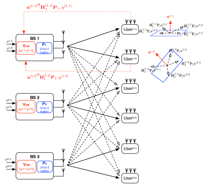
Figure 1: The MIMO IBC model, where $K=3$, $M=3$, $S=2$, $L=3$, and $N=2$.

III Proposed ODIA

We first describe the overall procedure of our proposed ODIA scheme for the MIMO IBC, and then define its achievable sum-rate and DoF.

III-A Overall Procedure

The ODIA scheme is described according to the following four steps.

III-A1 Initialization (Broadcast of Reference Beamforming Matrices)

First, as illustrated in Fig. 1, the precoding matrix at each BS is composed of the product of a predetermined reference beamforming matrix, denoted by $\mathbf{P}_{k}$, and a user-specific beamforming matrix, denoted by $\mathbf{V}_{k}$. In this step, we mainly focus on the design of $\mathbf{P}_{k}$. Specifically, the reference beamforming matrix at the BS in the $k$-th cell is given by $\mathbf{P}_{k}=\left[\mathbf{p}_{1,k},\ldots,\mathbf{p}_{S,k}\right]$, where $\mathbf{p}_{s,k}\in\mathbb{C}^{M\times 1}$ is an orthonormal basis for $k\in\mathcal{K}$ and $s=1,\ldots,S$. Each BS independently generates $\mathbf{p}_{k,s}$ according to the isotropic distribution over the $M$-dimensional unit sphere. If the reference beamforming matrix is generated in a pseudo-random fashion, BSs do not need to broadcast them to users. Then, the $j$-th user in the $i$-th cell obtains $\mathbf{H}^{[i,j]}_{k}$ and $\mathbf{P}_{k}$, $k=1,\ldots,K$.

III-A2 Receive Beamforming & Scheduling Metric Feedback

In the second step, we explain how to decide a user scheduling metric at each user along with given receive beamforming, where the design of receive beamforming will be explained in Section IV. Let $\mathbf{u}^{[i,j]}\in\mathbb{C}^{L\times 1}$ denote the unit-norm weight vector at the $j$-th user in the $i$-th cell, i.e., $\left\|\mathbf{u}^{[i,j]}\right\|^{2}=1$. Since the user-specific beamforming $\mathbf{V}_{k}$ will be utilized only to cancel intra-cell interference out, $\mathbf{V}_{k}$ does not change the inter-cell interference level at each user, which will be specified later. Thus, from the notion of $\mathbf{P}_{k}$ and $\mathbf{H}^{[i,j]}_{k}$, the $j$-th user in the $i$-th cell can compute the quantity of received interference from the $k$-th BS while using its receive beamforming vector $\mathbf{u}^{[i,j]}$, which is given by

$$\tilde{\eta}^{[i,j]}_{k} =\left\|{\mathbf{u}^{[i,j]}}^{\mathsf{H}}\mathbf{H}_{k}^{[i,j]}\mathbf{P}_{k}\right\|^{2},$$ (1)

where $i\in\mathcal{K}$, $j\in\mathcal{N}$, and $k\in\mathcal{K}\setminus i=\{1,\ldots,i-1,i+1,\ldots,K\}$. Using (1), the scheduling metric at the $j$-th user in the $i$-th cell, denoted by $\eta^{[i,j]}$, is defined as the sum of received interference power from other cells. That is,

$$\eta^{[i,j]} =\sum_{k=1,k\neq i}^{K}\tilde{\eta}^{[i,j]}_{k}.$$ (2)

As illustrated in Fig. 1, each user feeds the metric in (2) back to its home-cell BS. In addition to the scheduling metric in (2), each user needs to feed its effective channel vector back, so that the user-specific beamforming $\mathbf{V}_{k}$ is designed at each BS. The effective channel vector of the $j$-th user in the $i$-th cell is given by

$$\mathbf{f}_{i}^{[i,j]}\triangleq\left({\mathbf{u}^{[i,j]}}^{\mathsf{H}}\mathbf{H}^{[i,j]}_{i}\mathbf{P}_{i}\right)^{\mathsf{H}}.$$ (3)

III-A3 User Scheduling

Upon receiving $N$ users’ scheduling metrics in the serving cell, each BS selects $S$ users having the metrics up to the $S$-th smallest one. Without loss of generality, the indices of selected users in every cell are assumed to be $(1,\ldots,S)$. In this and subsequent sections, we focus on how to simply design a user scheduling method to guarantee the optimal DoF. An enhanced scheduling algorithm jointly taking into account the effective channel in (3) and the received interference level in (2) may provide a better performance in terms of sum-rate, which shall be discussed in Section VI.

III-A4 Transmit Beamforming & Downlink Data Transmission

The signal vector at the $i$-th BS transmitted to the $j$-th user in the $i$-th cell is given by $\mathbf{v}^{[i,j]}x^{[i,j]}$, where $x^{[i,j]}$ is the transmit symbol with power of $1/S$, and the user-specific beamforming matrix for $S$ users is given by $\mathbf{V}_{i}=\left[\mathbf{v}^{[i,1]},\ldots,\mathbf{v}^{[i,S]}\right]$, where $\mathbf{v}^{[i,s]}\in\mathbb{C}^{S\times 1}$, $i\in\mathcal{K}$. Denoting the transmit symbol vector of the $i$-th cell by $\mathbf{x}_{i}=\left[x^{[i,1]},\ldots,x^{[i,S]}\right]^{T}$, the received signal vector at the $j$-th user in the $i$-th cell is then written as

$$\mathbf{y}^{[i,j]} =\mathbf{H}_{i}^{[i,j]}\mathbf{P}_{i}\mathbf{V}_{i}\mathbf{x}_{i}+\sum_{k=1,k\neq i}^{K}\mathbf{H}_{k}^{[i,j]}\mathbf{P}_{k}\mathbf{V}_{k}\mathbf{x}_{k}+\mathbf{z}^{[i,j]}$$

$$=\underbrace{\mathbf{H}_{i}^{[i,j]}\mathbf{P}_{i}\mathbf{v}^{[i,j]}x^{[i,j]}}_{\textsf{desired signal}}+\underbrace{\sum_{s=1,s\neq j}^{S}\mathbf{H}_{i}^{[i,j]}\mathbf{P}_{i}\mathbf{v}^{[i,s]}x^{[i,s]}}_{\textsf{intra-cell interference}}$$

$$\hskip 20.0pt+\underbrace{\sum_{k=1,k\neq i}^{K}\mathbf{H}_{k}^{[i,j]}\mathbf{P}_{k}\mathbf{V}_{k}\mathbf{x}_{k}}_{\textsf{inter-cell interference}}+\mathbf{z}^{[i,j]},$$ (4)

where $\mathbf{z}^{[i,j]}\in\mathbb{C}^{L\times 1}$ denotes the additive white Gaussian noise vector, each element of which is i.i.d. complex Gaussian with zero mean and the variance of $\mathsf{{SNR}^{-1}}$. The received signal vector at the $j$-th user in the $i$-th cell after receive beamforming, denoted by $\tilde{y}^{[i,j]}={\mathbf{u}^{[i,j]}}^{\mathsf{H}}\mathbf{y}^{[i,j]}$, can be rewritten as:

$$\tilde{y}^{[i,j]} ={\mathbf{f}_{i}^{[i,j]}}^{\mathsf{H}}\mathbf{v}^{[i,j]}x^{[i,j]}+{\mathbf{f}_{i}^{[i,j]}}^{\mathsf{H}}\sum_{s=1,s\neq j}^{S}\mathbf{v}^{[i,s]}x^{[i,s]}$$

$$\hskip 10.0pt+\sum_{k=1,k\neq i}^{K}{\mathbf{f}_{k}^{[i,j]}}^{\mathsf{H}}\mathbf{V}_{k}\mathbf{x}_{k}+{\mathbf{u}^{[i,j]}}^{\mathsf{H}}\mathbf{z}^{[i,j]},$$ (5)

where ${\mathbf{f}_{k}^{[i,j]}}^{\mathsf{H}}={\mathbf{u}^{[i,j]}}^{\mathsf{H}}\mathbf{H}_{k}^{[i,j]}\mathbf{P}_{k}$. By selecting users with small $\eta^{[i,j]}$ in (2), $\mathbf{H}_{k}^{[i,j]}\mathbf{P}_{k}$ tends to be orthogonal to the receive beamforming vector $\mathbf{u}^{[i,j]}$; thus, inter-cell interference channel matrices $\mathbf{H}_{k}^{[i,j]}\mathbf{P}_{k}\mathbf{V}_{k}$ in (III-A4) also tend to be orthogonal to $\mathbf{u}^{[i,j]}$ as illustrated in Fig. 1.

To cancel out intra-cell interference, the user-specific beamforming matrix $\mathbf{V}_{i}\in\mathbb{C}^{S\times S}$is given by

$$\mathbf{V}_{i} =[\mathbf{v}^{[i,1]},\mathbf{v}^{[i,2]},\ldots,\mathbf{v}^{[i,S]}]$$

$$=\begin{bmatrix}{\mathbf{u}^{[i,1]}}^{\mathsf{H}}\mathbf{H}_{i}^{[i,1]}\mathbf{P}_{i}\\ {\mathbf{u}^{[i,2]}}^{\mathsf{H}}\mathbf{H}_{i}^{[i,2]}\mathbf{P}_{i}\\ \vdots\\ {\mathbf{u}^{[i,S]}}^{\mathsf{H}}\mathbf{H}_{i}^{[i,S]}\mathbf{P}_{i}\end{bmatrix}^{-1}\cdot\begin{bmatrix}\sqrt{\gamma^{[i,1]}}&0&\cdots&0\\ 0&\sqrt{\gamma^{[i,2]}}&\cdots&0\\ \vdots&\vdots&\ddots&\vdots\\ 0&0&\cdots&\sqrt{\gamma^{[i,S]}}\\ \end{bmatrix},$$ (6)

where $\sqrt{\gamma^{[i,j]}}$ denotes a normalization factor for satisfying the unit-transmit power constraint. In consequence, the received signal can be simplified to

$$\tilde{y}^{[i,j]} =\sqrt{\gamma^{[i,j]}}x^{[i,j]}$$

$$\hskip 20.0pt+\underbrace{\sum_{k=1,k\neq i}^{K}{\mathbf{f}_{k}^{[i,j]}}^{\mathsf{H}}\mathbf{V}_{k}\mathbf{x}_{k}}_{\textsf{inter-cell interference}}+{\mathbf{u}^{[i,j]}}^{\mathsf{H}}\mathbf{z}^{[i,j]},$$ (7)

which thus does not contain the intra-cell interference term.

As in [21, 22, 23, 24, 25, 13], we assume no loss in exchanging signaling messages such as information of effective channels, scheduling metrics, and receive beamforming vectors.

III-B Achievable Sum-Rate and DoF

From (III-A4), the achievable rate of the $j$-th user in the $i$-th cell is given by

$$R^{[i,j]} =\operatorname{log}_{2}\left(1+\frac{\gamma^{[i,j]}\cdot|x^{[i,j]}|^{2}}{\left|{{\mathbf{u}^{[i,j]}}^{\mathsf{H}}}\mathbf{z}^{[i,j]}\right|^{2}+\tilde{I}^{[i,j]}}\right)$$

$$=\operatorname{log}_{2}\left(1+\frac{\gamma^{[i,j]}}{\frac{S}{\mathsf{SNR}}+\sum_{k=1,k\neq i}^{K}\sum_{s=1}^{S}\left|{\mathbf{f}_{k}^{[i,j]}}^{\mathsf{H}}\mathbf{v}^{[k,s]}\right|^{2}}\right),$$ (8)

where $\tilde{I}^{[i,j]}\triangleq\sum_{k=1,k\neq i}^{K}\left|{\mathbf{f}_{k}^{[i,j]}}^{\mathsf{H}}\mathbf{V}_{k}\mathbf{x}_{k}\right|^{2}$. Using (III-B), the achievable total DoF can be defined as

$$\textrm{DoF}=\lim_{\textsf{SNR}\rightarrow\infty}\frac{\sum_{i=1}^{K}\sum_{j=1}^{S}R^{[i,j]}}{\operatorname{log}\textsf{SNR}}.$$ (9)

IV DoF Achievability

In this section, we characterize the DoF achievability in terms of the user scaling law with the optimal receive beamforming technique. To this end, we start with the receive beamforming design that maximizes the achievable DoF. For given channel instance, from (III-B), each user can attain the maximum DoF of 1 if and only if the interference $\sum_{k=1,k\neq i}^{K}\sum_{s=1}^{S}\Big{|}{\mathbf{f}_{k}^{[i,j]}}^{\mathsf{H}}\mathbf{v}^{[k,s]}\Big{|}^{2}\cdot\mathsf{SNR}$ remains constant for increasing SNR. Note that $R^{[i,j]}$ can be bounded as

$$R^{[i,j]}\geq\operatorname{log}_{2}\left(1+\frac{\gamma^{[i,j]}}{\frac{S}{\mathsf{SNR}}+\sum_{k=1,k\neq i}^{K}\sum_{s=1}^{S}\left\|\mathbf{f}_{k}^{[i,j]}\right\|^{2}\left\|\mathbf{v}^{[k,s]}\right\|^{2}}\right)$$ (10)

$$\geq\operatorname{log}_{2}\left(1+\frac{\gamma^{[i,j]}}{\frac{S}{\mathsf{SNR}}+\sum_{k\neq i}^{K}\sum_{s=1}^{S}\left\|\mathbf{f}_{k}^{[i,j]}\right\|^{2}\left\|\mathbf{v}^{(\operatorname{max})}_{i}\right\|^{2}}\right)$$ (11)

$$=\operatorname{log}_{2}\left(\mathsf{SNR}\right)+\operatorname{log}_{2}\left(\frac{1}{\mathsf{SNR}}+\frac{\frac{\gamma^{[i,j]}}{\left\|\mathbf{v}^{(\operatorname{max})}_{i}\right\|^{2}}}{\frac{S}{\left\|\mathbf{v}^{(\operatorname{max})}_{i}\right\|^{2}}+I^{[i,j]}}\right)$$ (12)

where $\mathbf{v}^{(\operatorname{max})}_{i}$ in (11) is defined by

$$\mathbf{v}^{(\operatorname{max})}_{i} =\operatorname{arg}\operatorname{max}\bigg{\{}\left\|\mathbf{v}^{[i^{\prime},j^{\prime}]}\right\|^{2}:i^{\prime}\in\mathcal{K}\setminus i,j^{\prime}\in\mathcal{S}\bigg{\}},$$ (13)

$\mathcal{S}\triangleq\{1,\ldots,S\}$, and $I^{[i,j]}$ in (12) is defined by

$$I^{[i,j]}\triangleq\sum_{k=1,k\neq i}^{K}\sum_{s=1}^{S}\left\|\mathbf{f}_{k}^{[i,j]}\right\|^{2}\cdot\mathsf{SNR}.$$ (14)

Here, $\mathbf{v}_{i}^{(\operatorname{max})}$ is fixed for given channel instance, because $\mathbf{v}^{[i,j]}$ is determined by $\mathbf{H}_{i}^{[i,j]}$, $j=1,\ldots,S$. Recalling that the indices of the selected users are $(1,\ldots,S)$ for all cells, we can expect the DoF of 1 for each user if and only if for some $0\leq\epsilon<\infty$,

$$I^{[i,j]}<\epsilon,\hskip 10.0pt\forall j\in\mathcal{S},i\in\mathcal{K}.$$ (15)

To maximize the achievable DoF, we aim to minimize the sum-interference $\sum_{i=1}^{K}\sum_{j=1}^{S}I^{[i,j]}$ through receive beamforming at the users. Since $I^{[i,j]}=\sum_{s=1}^{S}\eta^{[i,j]}\mathsf{SNR}$, we have

$$\sum_{i=1}^{K}\sum_{j=1}^{S}I^{[i,j]}=S\sum_{i=1}^{K}\sum_{j=1}^{S}\eta^{[i,j]}\mathsf{SNR}.$$ (16)

This implies that the collection of distributed effort to minimize $\eta^{[i,j]}$ at the users can reduce the sum of received interference. Therefore, each user finds the beamforming vector that minimizes $\eta^{[i,j]}$ from

$$\mathbf{u}^{[i,j]} =\operatorname{arg}\operatornamewithlimits{min}_{\mathbf{u}}\eta^{[i,j]}=\operatorname{arg}\operatornamewithlimits{min}_{\mathbf{u}}\sum_{k=1,k\neq i}^{K}\left\|\mathbf{u}^{\mathsf{H}}\mathbf{H}_{k}^{[i,j]}\mathbf{P}_{k}\right\|^{2}$$ (17)

$$=\operatorname{arg}\operatornamewithlimits{min}_{\mathbf{u}}\left\|\mathbf{G}^{[i,j]}\mathbf{u}\right\|^{2},$$ (18)

where

$$\mathbf{G}^{[i,j]} \triangleq\Bigg{[}\left(\mathbf{H}_{1}^{[i,j]}\mathbf{P}_{1}\right),\ldots,\left(\mathbf{H}_{i-1}^{[i,j]}\mathbf{P}_{i-1}\right),$$

$$\hskip 20.0pt\left(\mathbf{H}_{i+1}^{[i,j]}\mathbf{P}_{i+1}\right),\ldots,\left(\mathbf{H}_{K}^{[i,j]}\mathbf{P}_{K}\right)\Bigg{]}^{\mathsf{H}}\in\mathbb{C}^{(K-1)S\times L}.$$ (19)

Let us denote the singular value decomposition of $\mathbf{G}^{[i,j]}$ as

$$\mathbf{G}^{[i,j]}=\boldsymbol{\Omega}^{[i,j]}\boldsymbol{\Sigma}^{[i,j]}{\mathbf{V}^{[i,j]}}^{\mathsf{H}},$$ (20)

where $\boldsymbol{\Omega}^{[i,j]}\in\mathbb{C}^{(K-1)S\times L}$ and $\mathbf{V}^{[i,j]}\in\mathbb{C}^{L\times L}$ consist of $L$ orthonormal columns, and $\boldsymbol{\Sigma}^{[i,j]}=\textrm{diag}\left(\sigma^{[i,j]}_{1},\ldots,\sigma^{[i,j]}_{L}\right)$, where $\sigma^{[i,j]}_{1}\geq\cdots\geq\sigma^{[i,j]}_{L}$. Then, the optimal $\mathbf{u}^{[i,j]}$ is determined as

$$\mathbf{u}^{[i,j]}=\mathbf{v}^{[i,j]}_{L},$$ (21)

where $\mathbf{v}^{[i,j]}_{L}$ is the $L$-th column of $\mathbf{V}^{[i,j]}$. With this choice the scheduling metric is simplified to

$$\eta^{[i,j]}={\sigma^{[i,j]}_{L}}^{2}.$$ (22)

Since each column of $\mathbf{P}_{k}$ is isotropically and independently distributed, each element of the effective interference channel matrix $\mathbf{G}^{[i,j]}$ is i.i.d. complex Gaussian with zero mean and unit variance.

We start with the following lemma for the probabilistic interference level of the ODIA, which shall be frequently used in the sequel.

Lemma 1

The sum-interference remains constant with high probability for increasing SNR, that is,

$$\lim_{\textsf{SNR}\rightarrow\infty}\mathcal{P} \triangleq\lim_{\textsf{SNR}\rightarrow\infty}\textrm{Pr}\Bigg{\{}\sum_{i=1}^{K}\sum_{j=1}^{S}I^{[i,j]}\leq\epsilon\Bigg{\}}=1$$ (23)

for any $0<\epsilon<\infty$, if

$$N=\omega\left(\mathsf{SNR}^{(K-1)S-L+1}\right).$$ (24)

Proof:

Since the cumulative density function (CDF) of $\eta^{[i,j]}$ is the same as that of the scheduling metric of the MIMO IMAC [14], the lemma can be readily proved by following the footsteps of Lemma 1 and Theorem 2 of [14]. ∎

Now, the following theorem establishes the DoF achievability of the proposed ODIA.

Theorem 1 (User scaling law)

The proposed ODIA scheme with the scheduling metric (22) achieves the optimal $KS$ DoF for given $S$ with high probability if

$$N=\omega\left(\textsf{SNR}^{(K-1)S-L+1}\right).$$ (25)

Proof:

If the sum-interference remains constant with probability $\mathcal{P}$ as defined in (23), the achievable rate in (12) can be further bounded by

$$R^{[i,j]} \geq\left[\operatorname{log}_{2}\left(\mathsf{SNR}\right)+\operatorname{log}_{2}\left(\frac{1}{\mathsf{SNR}}+\frac{\frac{\gamma^{[i,j]}}{\left\|\mathbf{v}^{(\operatorname{max})}_{i}\right\|^{2}}}{\frac{S}{\left\|\mathbf{v}^{(\operatorname{max})}_{i}\right\|^{2}}+\epsilon}\right)\right]\cdot\mathcal{P},$$ (26)

for any $0\leq\epsilon<\infty$. Thus, the achievable DoF can be bounded by

$$\textrm{DoF}=\lim_{\textsf{SNR}\rightarrow\infty}\frac{\sum_{i=1}^{K}\sum_{j=1}^{S}R^{[i,j]}}{\operatorname{log}\textsf{SNR}}\geq\lim_{\textsf{SNR}\rightarrow\infty}KS\cdot\mathcal{P}.$$ (27)

From Lemma 1, it is immediate to show that $\mathcal{P}$ tends to 1, and hence $KS$ DoF is achievable if $N=\omega\left(\mathsf{SNR}^{(K-1)S-L+1}\right)$, which proves the theorem. ∎

Compared to the previous results of $N=\omega\left(\mathsf{SNR}^{KS-L}\right)$ [15, 19, 20], the exponent of SNR is reduced by $S-1$ using the proposed ODIA, owing to perfect CSI of the selected users at each BS, resulting in a slightly increased overhead. The essence of the ODIA is that the design of the precoder $\mathbf{V}_{i}$ can be decoupled from the design of the receive beamforming vector $\mathbf{u}^{[i,j]}$, because the scheduling metric $\eta^{[i,j]}$ is calculated at the user side in a distributed fashion without the knowledge of $\mathbf{V}_{i}$. Even with this decoupled approach, interference can still be minimized due to the cascaded precoder design. As a result, optimal DoF can be achieved without any iterative precoder and receive beamforming vector optimization as done in [4]. In addition, the proposed ODIA applies to arbitrary $M$, $L$, and $K$, whereas the optimal DoF is achievable only in a few special cases in the scheme proposed in [4].

The following remark discusses the uplink and downlink duality within the OIA framework.

Remark 1 (Uplink-downlink duality)

The same scaling condition of $N=\omega\left(\mathsf{SNR}^{K(S-1)-L+1}\right)$ was achieved to obtain $KS$ DoF in the uplink interference channel [14]. Therefore, Theorem 1 implies that a duality holds true for the uplink and downlink OIA frameworks in terms of the user scaling law.

The user scaling law characterizes the trade-off between the asymptotic DoF and number of users, i.e., the more number of users, the more achievable DoF. In addition, we relate the derived user scaling law to the interference decaying rate with respect to $N$ for given SNR. We start with the following lemma.

Lemma 2

The interference decaying rate of a selected $j$th user in the $i$-th cell with respect to $N$ is given by

$$E\left\{\frac{1}{\eta^{[i,j]}}\right\}\geq\Theta\left(N^{1/((K-1)S-L+1)}\right).$$ (28)

Here, $f(x)=\Theta(g(x))$ if $f(x)=O(g(x))$ and $g(x)=O(f(x))$.

Proof:

The lemma can be shown by following the footsteps of the proof of [16, Theorem 3]. The detailed proof is provided in Appendix A. ∎

Theorem 2 (Interference decaying rate)

If the user scaling condition to achieve a target DoF is given by $N=\omega\left(\textsf{SNR}^{\tau^{\prime}}\right)$ for some $\tau^{\prime}>0$, then the interference decaying rate is given by

$$E\left\{\frac{1}{\eta^{[i,j]}}\right\}\geq\Theta\left(N^{1/\tau^{\prime}}\right).$$ (29)

Proof:

Since both the user scaling law and interference decaying rate are determined by the tail CDF of the scheduling metric, the theorem can be readily proved by the proofs of Theorem 1 and Lemma 2. ∎

Therefore, from Theorem 2, the user scaling law also provides an insight on the interference decaying rate with respect to $N$ for given SNR; that is, the smaller SNR exponent of the user scaling law, the faster interference decreasing rate with respect to $N$.

V ODIA with Limited feedback

In the proposed ODIA scheme, the effective channel vectors (${\mathbf{u}^{[i,j]}}^{\mathsf{H}}\mathbf{H}^{[i,j]}_{i}\mathbf{P}_{i}$) in (3) can be fed back to the corresponding BS using pilots rotated by the effective channels [26]. However, this analog feedback requires two consecutive pilot phases for each user: regular pilot for uplink channel estimation and analog feedback for effective channel estimation. Hence, pilot overhead grows with respect to the number of users in the network. As a result, in practical systems with massive users, it is more preferable to follow the widely-used limited feedback approach [27], in which effective channels are fed back using codebooks.

For limited feedback of effective channel vectors, we define the codebook by

$$\mathcal{C}_{f}=\left\{\mathbf{c}_{1},\ldots,\mathbf{c}_{N_{f}}\right\},$$ (30)

where $N_{f}$ is the codebook size and $\mathbf{c}_{k}\in\mathbb{C}^{S\times 1}$ is a unit-norm codeword, i.e., $\|\mathbf{c}_{i}\|^{2}=1$. Hence, the number of feedback bits used is given by

$$n_{f}=\lceil\operatorname{log}_{2}N_{f}\rceil(\textrm{bits})$$ (31)

For the effective channel ${\mathbf{f}_{i}^{[i,j]}}^{\mathsf{H}}={\mathbf{u}^{[i,j]}}^{\mathsf{H}}\mathbf{H}^{[i,j]}_{i}\mathbf{P}_{i},$ each user quantizes the normalized effective channel for given $\mathcal{C}_{f}$ from

$$\mathbf{f}_{i}^{[i,j]}=\operatorname{arg}\operatorname{max}_{\{\mathbf{w}=\mathbf{c}_{k}:1\leq k\leq N_{f}\}}\frac{\left|{\mathbf{f}_{i}^{[i,j]}}^{\mathsf{H}}\mathbf{w}\right|^{2}}{\left\|\mathbf{f}_{i}^{[i,j]}\right\|^{2}}.$$ (32)

Now, the user feeds back three types of information: 1) index of $\mathbf{f}_{i}^{[i,j]}$, 2) channel gain of $\left\|\mathbf{f}_{i}^{[i,j]}\right\|^{2}$, and 3) scheduling metric $\eta^{[i,j]}$. Note that the channel gains and scheduling metrics are real scalar values, and thus can be accurately fed back as uplink data. Then, BS $i$ constructs the quantized effective channel vectors $\hat{\mathbf{f}}^{[i,j]}$ from

$$\hat{\mathbf{f}}^{[i,j]}\triangleq\left\|\mathbf{f}_{i}^{[i,j]}\right\|^{2}\cdot\mathbf{f}_{i}^{[i,j]},\hskip 10.0pti=1,\ldots,S,$$ (33)

and the precoding matrix $\hat{\mathbf{V}}_{i}$ from

$$\hat{\mathbf{V}}_{i}=\hat{\mathbf{F}}_{i}^{-1}\boldsymbol{\Gamma}_{i},$$ (34)

where $\boldsymbol{\Gamma}_{i}=\textrm{diag}\left(\sqrt{\gamma^{[i,1]}},\ldots,\sqrt{\gamma^{[i,S]}}\right)$ and $\hat{\mathbf{F}}_{i}=\left[\hat{\mathbf{f}}^{[i,1]},\ldots,\hat{\mathbf{f}}^{[i,S]}\right]^{\mathsf{H}}$.

With limited feedback, the received signal vector after receive beamforming is written by

$$\tilde{y}^{[i,j]} ={\mathbf{f}_{i}^{[i,j]}}^{\mathsf{H}}\hat{\mathbf{V}}_{i}\mathbf{x}_{i}+\cdot\sum_{k=1,k\neq i}^{K}{\mathbf{f}_{k}^{[i,j]}}^{\mathsf{H}}\hat{\mathbf{V}}_{k}\mathbf{x}_{k}$$

$$\hskip 50.0pt+{\mathbf{u}^{[i,j]}}^{\mathsf{H}}\mathbf{z}^{[i,j]}$$ (35)

$$=\sqrt{\gamma^{[i,j]}}x^{[i,j]}+\underbrace{\left({\mathbf{f}_{i}^{[i,j]}}^{\mathsf{H}}\hat{\mathbf{V}}_{i}\mathbf{x}_{i}-\sqrt{\gamma^{[i,j]}}x^{[i,j]}\right)}_{\textrm{residual intra-cell interference}}$$

$$\hskip 20.0pt+\sum_{k=1,k\neq i}^{K}{\mathbf{f}_{k}^{[i,j]}}^{\mathsf{H}}\hat{\mathbf{V}}_{k}\mathbf{x}_{k}+{\mathbf{u}^{[i,j]}}^{\mathsf{H}}\mathbf{z}^{[i,j]},$$ (36)

where the residual intra-cell interference is non-zero due to the quantization error in $\hat{\mathbf{V}}_{i}$.

It is important to note that the residual intra-cell interference is a function of $\hat{\mathbf{V}}_{i}$, which includes other users’ channel information, and thus each user treats this term as unpredictable noise and calculates only the inter-cell interference for the scheduling metric as in (2); that is, the scheduling metric is not changed for the ODIA with limited feedback.

The following theorem establishes the user scaling law for the ODIA with limited feedback.

Theorem 3

The ODIA with a Grassmannian or random codebook achieves the same user scaling law of the ODIA with perfect CSI described in Theorem 1, if

$$n_{f}=\omega\left(\operatorname{log}_{2}\mathsf{SNR}\right).$$ (37)

That is, $KS$ DoF is achievable with high probability if $N=\omega\left(\mathsf{SNR}^{(K-1)S-L+1}\right)$ and (37) holds true.

Proof:

Without loss of generality, the quantized effective channel vector $\hat{\mathbf{f}}^{[i,j]}$ can be decomposed as

$$\hat{\mathbf{f}}^{[i,j]} =\left\|\mathbf{f}_{i}^{[i,j]}\right\|^{2}\cdot\mathbf{f}_{i}^{[i,j]}$$

$$=\sqrt{1-{d^{[i,j]}}^{2}}\cdot\mathbf{f}_{i}^{[i,j]}+d^{[i,j]}\left\|\mathbf{f}_{i}^{[i,j]}\right\|^{2}\left(\mathbf{t}^{[i,j]}\right),$$ (38)

where $\mathbf{t}^{[i,j]}$ is a unit-norm vector i.i.d. over $\textrm{null}\left(\mathbf{f}_{i}^{[i,j]}\right)$ [21]. At this point, we consider the worse performance case where each user finds $\hat{\mathbf{f}}^{[i,j]}$ such that with a slight abuse of notation

$$\hat{\mathbf{f}}^{[i,j]}=\sqrt{1-{d^{\operatorname{max}}_{i}}^{2}}\cdot\mathbf{f}_{i}^{[i,j]}+d^{\operatorname{max}}_{i}\nu_{i}\cdot\mathbf{t}^{[i,j]},$$ (39)

where

$$d^{\operatorname{max}}_{i}=\operatorname{max}\left\{d^{[i,1]},\ldots,d^{[i,S]}\right\},$$ (40)

$$\nu_{i}=\operatorname{max}\left\{\left\|\mathbf{f}_{i}^{[i,j]}\right\|^{2},j=1,\ldots,S\right\}.$$ (41)

Note that more quantization error only degrades the achievable rate, and hence the quantization via (39) yields a performance lower-bound. Inserting (39) to (34) gives us

$$\hat{\mathbf{V}}_{i}=\left(\sqrt{1-{d^{\operatorname{max}}_{i}}^{2}}\mathbf{F}_{i}+d^{\operatorname{max}}_{i}\nu_{i}\mathbf{T}_{i}\right)^{-1}\boldsymbol{\Gamma}_{i},$$ (42)

where ${\mathbf{F}}_{i}=\left[\mathbf{f}_{i}^{[i,1]},\ldots,\mathbf{f}_{i}^{[i,S]}\right]^{\mathsf{H}}$ and ${\mathbf{T}}_{i}=\left[{\mathbf{t}}^{[i,1]},\ldots,{\mathbf{t}}^{[i,S]}\right]^{\mathsf{H}}$.

The Taylor expansion of $\left(\sqrt{1-{d^{\operatorname{max}}_{i}}^{2}}\mathbf{F}_{i}+d^{\operatorname{max}}_{i}\nu_{i}\mathbf{T}\right)^{-1}$ in (34) gives us

$$\left(\sqrt{1-{d^{\operatorname{max}}_{i}}^{2}}\mathbf{F}_{i}+d^{\operatorname{max}}_{i}\nu_{i}\mathbf{T}_{i}\right)^{-1}$$

$$\hskip 20.0pt=\mathbf{F}_{i}^{-1}-\mathbf{F}_{i}^{-1}\mathbf{T}_{i}\mathbf{F}_{i}^{-1}\nu_{i}d^{\operatorname{max}}_{i}+\sum_{k=2}^{\infty}\mathbf{A}_{k}\left(d^{\operatorname{max}}_{i}\right)^{k},$$ (43)

where $\mathbf{A}_{k}$ is a function of $\mathbf{F}_{i}$ and $\mathbf{T}_{i}$. Thus, $\hat{\mathbf{V}}_{i}$ can be written by

$$\hat{\mathbf{V}}_{i}=\mathbf{F}_{i}^{-1}\boldsymbol{\Gamma}_{i}-d^{\operatorname{max}}_{i}\nu_{i}\mathbf{F}_{i}^{-1}\mathbf{T}_{i}\mathbf{F}_{i}^{-1}\boldsymbol{\Gamma}_{i}+\sum_{k=2}^{\infty}\left(d^{\operatorname{max}}_{i}\right)^{k}\mathbf{A}_{k}\boldsymbol{\Gamma}_{i}$$ (44)

Inserting (44) to (V) yields

$$\tilde{y}^{[i,j]} =\sqrt{\gamma^{[i,j]}}x^{[i,j]}$$

$$\underbrace{-d^{\operatorname{max}}_{i}\nu_{i}{\mathbf{t}^{[i,j]}}^{\textsf{H}}\mathbf{F}_{i}^{-1}\boldsymbol{\Gamma}_{i}\mathbf{x}_{i}+\sum_{k=2}^{\infty}\left(d^{\operatorname{max}}_{i}\right)^{k}{\mathbf{f}_{i}^{[i,j]}}^{\mathsf{H}}\mathbf{A}_{k}\boldsymbol{\Gamma}_{i}\mathbf{x}_{i}}_{\textrm{residual intra-cell interference}}$$

$$+\sum_{k=1,k\neq i}^{K}{\mathbf{f}_{k}^{[i,j]}}^{\mathsf{H}}\hat{\mathbf{V}}_{k}\mathbf{x}_{k}+{\mathbf{u}^{[i,j]}}^{\mathsf{H}}\mathbf{z}^{[i,j]}.$$ (45)

Consequently, the rate $R^{[i,j]}$ in (III-B) is given by

$$R^{[i,j]}=\operatorname{log}_{2}\left(1+\frac{\gamma^{[i,j]}}{\frac{S+\Delta^{[i,j]}}{\mathsf{SNR}}+\sum_{k\neq i}^{K}\sum_{s=1}^{S}\left|{\mathbf{f}_{k}^{[i,j]}}^{\mathsf{H}}\mathbf{v}^{[k,s]}\right|^{2}}\right),$$ (46)

where

$$\Delta^{[i,j]}=\left(d^{\operatorname{max}}_{i}\right)^{2}\delta_{1}\cdot\mathsf{SNR}+\sum_{k=2}^{\infty}\left(d^{\operatorname{max}}_{i}\right)^{2k}\delta_{k}\cdot\mathsf{SNR},$$ (47)

$$\delta_{1}=\left(\nu_{i}^{2}{\mathbf{t}^{[i,j]}}^{\textsf{H}}\mathbf{F}_{i}^{-1}{\boldsymbol{\Gamma}_{i}}^{2}\mathbf{F}_{i}^{-\mathsf{H}}\mathbf{t}^{[i,j]}\right),$$ (48)

$$\delta_{k}=\left({\mathbf{f}_{i}^{[i,j]}}^{\mathsf{H}}\mathbf{A}_{k}\boldsymbol{\Gamma}_{i}^{2}\mathbf{A}_{k}^{\mathsf{H}}\mathbf{f}_{i}^{[i,j]}\right)$$ (49)

As in (10) to (12), the achievable rate can be bounded by

$$R^{[i,j]} \geq\left[\operatorname{log}_{2}\left(\mathsf{SNR}\right)+\operatorname{log}_{2}\left(\frac{1}{\mathsf{SNR}}+\frac{\frac{\gamma^{[i,j]}}{\left\|\mathbf{v}^{(\operatorname{max})}_{i}\right\|^{2}}}{\frac{1}{\left\|\mathbf{v}^{(\operatorname{max})}_{i}\right\|^{2}}+2\epsilon}\right)\right]\cdot\mathcal{P}^{\prime},$$ (50)

where

$$\mathcal{P}^{\prime} \triangleq\textrm{Pr}\Bigg{\{}\left(\sum_{i=1}^{K}\sum_{j=1}^{S}I^{[i,j]}\leq\epsilon\right)\&\left(\Delta^{[i,j]}/\left\|\mathbf{v}^{(\operatorname{max})}_{i}\right\|^{2}\leq\epsilon\right),$$

$$\hskip 80.0pt\forall i\in\mathcal{K},j\in\mathcal{S}\Bigg{\}}$$ (51)

$$=\textrm{Pr}\Bigg{\{}\sum_{i=1}^{K}\sum_{j=1}^{S}I^{[i,j]}\leq\epsilon,\forall i\in\mathcal{K},j\in\mathcal{S}\Bigg{\}}$$

$$\hskip 50.0pt\times\textrm{Pr}\Bigg{\{}\Delta^{[i,j]}\leq\epsilon^{\prime},\forall i\in\mathcal{K},j\in\mathcal{S}\Bigg{\}},$$ (52)

where $\epsilon^{\prime}\triangleq\epsilon\cdot\left\|\mathbf{v}^{(\operatorname{max})}_{i}\right\|^{2}$. Here, (V) follows from the fact that the inter-cell interference $I^{[i,j]}$ and residual intra-cell interference $\Delta^{[i,j]}$ are independent each other. Note also that the level of residual intra-cell interference does not affect the user selection and is determined only by the codebook size $N_{f}$. Hence, the user selection result does not change for different $N_{f}$.

The achievable DoF is given by

$$\textrm{DoF}\geq\lim_{\textsf{SNR}\rightarrow\infty}KS\cdot\mathcal{P}^{\prime}.$$ (53)

If $N=\omega\left(\textsf{SNR}^{(K-1)S-L+1}\right)$, the first term of (V) tends to 1 according to Lemma 1. Thus, the maximum DoF can be obtained if and only if $\Delta^{[i,j]}\leq\epsilon^{\prime}$ for all selected users for increasing SNR.

In Appendix B, it is shown that $\Delta^{[i,j]}\leq\epsilon^{\prime}$ for all selected users if $n_{f}=\omega\left(\operatorname{log}_{2}\mathsf{SNR}\right)$ for both Grassmannian and random codebooks. Therefore, if $N=\omega\left(\textsf{SNR}^{(K-1)S-L+1}\right)$ and $n_{f}=\omega\left(\operatorname{log}_{2}\mathsf{SNR}\right)$, $\mathcal{P}^{\prime}$ in (V) tends to 1, which proves the theorem. ∎

From Theorem 3, the minimum number of feedback bits $n_{f}$ is characterized to achieve the optimal $KS$ DoF, which increases with respect to $\operatorname{log}_{2}(\mathsf{SNR})$. It is worthwhile to note that the results are the same for the Grassmannian and random codebooks. In the previous works on limited feedback systems, the performance analysis was focused on the average SNR or the average rate loss [28]. In an average sense, the Grassmannian codebook is in general outperforms the random codebook. However, our scheme focuses on the asymptotic codebook performance for given channel instance for increasing SNR, and it turned out that this asymptotic behaviour is the same for the two codebooks. In fact, this result agrees with the previous works e.g., [29], in which the performance gap between the two codebooks was shown to be negligible as $n_{f}$ increases through computer simulations.

We conclude this section by providing the following comparison to the well-known conventional result on limited feedback systems.

Remark 2

For the MIMO broadcast channel with limited feedback, where the transmitter has $L$ antennas and employs the random codebook, it was shown [21] that the achievable rate loss for each user, denoted by $\Delta R$, due to the finite size of the codebook is lower-bounded by

$$\Delta<\operatorname{log}_{2}\left(1+\textrm{SNR}\cdot 2^{-n_{f}/(L-1)}\right).$$ (54)

Thus, to achieve the maximum 1 DoF for each user, or to make the rate loss negligible as the SNR increases, the term $\textrm{SNR}\cdot 2^{-n_{f}/(L-1)}$ should remain constant for increasing SNR. That is, $n_{f}$ should scale faster than $(L-1)\operatorname{log}_{2}(\textrm{SNR})$. Though the system is different, our results of Theorem 3 are consistent with this previous result.

VI Spectrally Efficient ODIA (SE-ODIA)

In this section, we propose a spectrally efficient OIA (SE-ODIA) scheme and show that the proposed SE-ODIA achieves the optimal multiuser diversity gain $\operatorname{log}\operatorname{log}N$. For the DoF achievability, it was enough to design the user scheduling in the sense to minimize inter-cell interference. However, to achieve optimal multiuser diversity gain, the gain of desired channels also needs to be considered in user scheduling. The overall procedure of the SE-ODIA follows that of the ODIA described in Section III except the the third stage ‘User Scheduling’. In addition, we assume the perfect feedback of the effective desired channels ${\mathbf{u}^{[i,j]}}^{\mathsf{H}}\mathbf{H}_{i}^{[i,j]}\mathbf{P}_{i}$ for the SE-ODIA. We incorporate the semiorthogonal user selection algorithm proposed in [30] to the ODIA framework taking into consideration inter-cell interference. Specifically, the algorithm for the user scheduling at the BS side is as follows:

• Step 1: Initialization:

  $$\mathcal{N}_{1} =\{1,\ldots,N\},\hskip 10.0pts=1$$ (55)

• Step 2: For each user $j\in\mathcal{N}_{s}$ in the $i$-th cell, the $s$-th orthogonal projection vector, denoted by $\tilde{\mathbf{b}}_{s}^{[i,j]}$, for given $\left\{\mathbf{b}_{1}^{[i]},\ldots,\mathbf{b}_{s-1}^{[i]}\right\}$ is calculated from:

  $$\tilde{\mathbf{b}}^{[i,j]}_{s} =\mathbf{f}_{i}^{[i,j]}-\sum_{s^{\prime}=0}^{s-1}\frac{{\mathbf{b}_{s^{\prime}}^{[i]}}^{\mathsf{H}}\mathbf{f}_{i}^{[i,j]}}{\|\mathbf{b}_{s^{\prime}}^{[i]}\|^{2}}\mathbf{b}_{s^{\prime}}^{[i]}$$ (56)

  Note that if $s=1$, $\tilde{\mathbf{b}}_{1}^{[i,j]}=\mathbf{f}_{i}^{[i,j]}$.

• Step 3: For the $s$-th user selection, a user is selected at random from the user pool $\mathcal{N}_{s}$ that satisfies the following two conditions:

  $$\mathsf{C}_{1}: \eta^{[i,j]}\leq\eta_{I},\hskip 10.0pt\mathsf{C}_{2}:\|\tilde{\mathbf{b}}_{s}^{[i,j]}\|^{2}\geq\eta_{D}$$ (57)

  Denote the index of the selected user by $\pi(s)$ and define

  $$\mathbf{b}_{s}^{[i]}=\tilde{\mathbf{b}}^{[i,\pi(s)]}_{s}.$$ (58)

• Step 4: If $s<S$, then find the $(s+1)$-th user pool $\mathcal{N}_{s+1}$ from:

  $$\mathcal{N}_{s+1} =\left\{j:j\in\mathcal{N}_{s},j\neq\pi(s),\frac{\left|{\mathbf{f}_{i}^{[i,j]}}^{\mathsf{H}}\mathbf{b}_{s}^{[i]}\right|}{\|\mathbf{f}_{i}^{[i,j]}\|\|\mathbf{b}_{s}^{[i]}\|}<\alpha\right\},\hskip 10.0pt$$ (59)

  $$s =s+1,$$ (60)

  where $\alpha>0$ is a positive constant. Repeat Step 2 to Step 4 until $s=S$.

To show the SE-ODIA achieves the optimal multiuser diversity gain, we start with the following lemma for the bound on $|\mathcal{N}_{s}|$.

Lemma 3

The cardinality of $\mathcal{N}_{s}$ can be bounded by

$$|\mathcal{N}_{s}| \gtrsim N\cdot\alpha^{2(S-1)}.$$ (61)

The approximated inequality becomes tight as $N$ increases.

Proof:

See Appendix C. ∎

We also introduce the following useful lemma.

Lemma 4

If $x\in\mathbb{C}^{M\times 1}$ has its element i.i.d. according to $\mathcal{CN}(0,\sigma^{2})$ and $\mathbf{A}$ is an idempotent matrix of rank $r$ (i.e., $\mathbf{A}^{2}=\mathbf{A}$), then $\mathbf{x}^{\mathsf{H}}\mathbf{A}\mathbf{x}/\sigma^{2}$ has a Chi-squared distribution with $2r$ degrees-of-freedom.

Proof:

See [31]. ∎

In addition, the following lemma on the achievable rate of the SE-ODIA will be used to show the achievability of optimal multiuser diversity gain.

Lemma 5

For the $j$-th selected user in the $i$-th cell, the achievable rate is bounded by

$$R^{[i,j]}\geq\operatorname{log}_{2}\left(1+\frac{\frac{\left\|\mathbf{b}_{j}^{[i]}\right\|^{2}}{1+\frac{(S-1)^{4}\alpha^{2}}{1-(S-1)\alpha^{2}}}}{\frac{S}{\mathsf{SNR}}+\sum_{k\neq i}^{K}\sum_{s=1}^{S}\left|{\mathbf{f}_{k}^{[i,j]}}^{\mathsf{H}}\mathbf{v}^{[k,s]}\right|^{2}}\right).$$ (62)

Proof:

Since the chosen channel vectors are not perfectly orthogonal, there is degradation in the effective channel gain $\gamma^{[i,j]}$. Specifically, for the $j$-th selected user in the $i$-th cell, we have

$$\gamma^{[i,j]} =\frac{1}{\left[\left(\mathbf{F}_{i}\mathbf{F}_{i}^{\mathsf{H}}\right)^{-1}\right]_{j,j}}>\frac{\left\|\mathbf{b}_{j}^{[i]}\right\|^{2}}{1+\frac{(S-1)^{4}\alpha^{2}}{1-(S-1)\alpha^{2}}},$$ (63)

which follows from [30, Lemma 2]. Inserting (63) to the sum-rate lower bound in (III-B) proves the lemma. ∎

Now the following theorem establishes the achievability of the optimal multiuser diversity gain.

Theorem 4

The proposed SE-ODIA scheme with

$$\eta_{D}=\epsilon_{D}\operatorname{log}\mathsf{SNR}$$ (64)

$$\eta_{I}=\epsilon_{I}\mathsf{SNR}^{-1}$$ (65)

for any $\epsilon_{D},\epsilon_{I}>0$ achieves the optimal multiuser diversity gain given by

$$R^{[i,j]}=\Theta\left(\operatorname{log}\left(\mathsf{SNR}\cdot\operatorname{log}N\right)\right),$$ (66)

with high probability for all selected users in the high SNR regime if

$$N=\omega\left(\mathsf{SNR}^{\frac{(K-1)S-L+1}{1-(\epsilon_{D}/2)}}\right).$$ (67)

Proof:

Amongst $|\mathcal{N}_{s}|$ users, there should exist at least one user satisfying the conditions $\mathsf{C}_{1}$ and $\mathsf{C}_{2}$ to make the proposed user scheduling for the SE-ODIA valid. Thus, we first show the probability that there exist at least one valid user, denoted by $\mathsf{p}_{s}$, converges to 1, for the $s$-th user selection, if $N$ scales according to (67) with the choices (64) and (65).

The probability that each user satisfies the two conditions is given by $\textrm{Pr}\left\{\mathsf{C}_{1}\right\}\cdot\textrm{Pr}\left\{\mathsf{C}_{2}\right\}$, because the two conditions are independent of each other. Consequently, $\mathsf{p}_{s}$ is given by

$$\mathsf{p}_{s} =1-\left(1-\textrm{Pr}\left\{\mathsf{C}_{1}\right\}\cdot\textrm{Pr}\left\{\mathsf{C}_{2}\right\}\right)^{|\mathcal{N}_{s}|}$$ (68)

$$\gtrsim 1-\left(1-\textrm{Pr}\left\{\mathsf{C}_{1}\right\}\cdot\textrm{Pr}\left\{\mathsf{C}_{2}\right\}\right)^{N\cdot\alpha^{2(S-1)}}.$$ (69)

Note that each element of ${\mathbf{f}_{i}^{[i,j]}}^{\mathsf{H}}={\mathbf{u}^{[i,j]}}^{\mathsf{H}}\mathbf{H}^{[i,j]}_{i}\mathbf{P}_{i}$ is i.i.d. according to $\mathcal{CN}(0,1)$, because each column of $\mathbf{P}_{i}$ is a random orthogonal unit vector and because ${\mathbf{u}^{[i,j]}}^{\mathsf{H}}$ is designed independently of $\mathbf{H}_{i}^{[i,j]}$ and isotropically distributed over a unit sphere. Thus, ${\mathbf{f}_{i}^{[i,j]}}^{\mathsf{H}}={\mathbf{u}^{[i,j]}}^{\mathsf{H}}\mathbf{H}^{[i,j]}_{i}\mathbf{P}_{i}$ has its element i.i.d. according to $\mathcal{CN}(0,1)$.

Let us define $\mathbf{P}$ by

$$\mathbf{P} \triangleq\left(\mathbf{I}-\sum_{s^{\prime}=0}^{s-1}\frac{\mathbf{b}_{s^{\prime}}^{[i]}{\mathbf{b}_{s^{\prime}}^{[i]}}^{\mathsf{H}}}{\|\mathbf{b}_{s^{\prime}}^{[i]}\|^{2}}\right),$$ (70)

which is a symmetric idempotent matrix with rank $(S-s+1)$. Since $\mathbf{b}_{s}^{[i]}=\mathbf{P}\mathbf{f}_{i}^{[i,j]}$, from Lemma 4, $\left\|\mathbf{b}_{s}^{[i]}\right\|^{2}$ is a Chi-squared random variable with $2(S-s+1)$ degrees-of-freedom.

In Appendix D, for $\eta_{D}>2$, we show that

$$\lim_{\mathsf{SNR}\rightarrow\infty}\mathsf{p}_{s}=1,\hskip 10.0pt\textrm{if }N=\omega\left(\mathsf{SNR}^{\frac{(K-1)S-L+1}{1-(\epsilon_{D}/2)}}\right).$$ (71)

Now, given that there always exist at least one user that satisfies the conditions $\mathsf{C}_{1}$ and $\mathsf{C}_{2}$, the achievable sum-rate can be bounded from Lemma 5 by

$$R^{[i,j]} \geq\operatorname{log}_{2}\left(1+\frac{\frac{\left\|\mathbf{b}_{j}^{[i]}\right\|^{2}}{1+\frac{(S-1)^{4}\alpha^{2}}{1-(S-1)\alpha^{2}}}\cdot\frac{1}{\left\|\mathbf{v}_{i}^{\operatorname{max}}\right\|^{2}}}{\frac{S}{\mathsf{SNR}\left\|\mathbf{v}_{i}^{\operatorname{max}}\right\|^{2}}+\sum_{k\neq i}^{K}\sum_{s=1}^{S}\left\|\mathbf{f}_{k}^{[i,j]}\right\|^{2}}\right)$$ (72)

$$\geq\operatorname{log}_{2}\left(1+\frac{\frac{\left\|\mathbf{b}_{j}^{[i]}\right\|^{2}}{1+\frac{(S-1)^{4}\alpha^{2}}{1-(S-1)\alpha^{2}}}\cdot\mathsf{SNR}/\left\|\mathbf{v}_{i}^{\operatorname{max}}\right\|^{2}}{S/\left\|\mathbf{v}_{i}^{\operatorname{max}}\right\|^{2}+KS\epsilon_{I}}\right)$$ (73)

$$=\operatorname{log}_{2}\left(1+\left\|\mathbf{b}_{j}^{[i]}\right\|^{2}\mathsf{SNR}\cdot\xi\right)$$ (74)

$$\geq\operatorname{log}_{2}\left(1+\epsilon_{D}(\operatorname{log}N)\cdot\mathsf{SNR}\right),$$ (75)

where (73) follows from the fact that the sum-interference for all selected users, given by $\sum_{j=1}^{S}\sum_{i=1}^{K}\eta^{[i,j]}\mathsf{SNR}$ (See (16)), does not exceed $KS\epsilon_{I}$ by choosing $\eta_{I}=\epsilon_{I}\mathsf{SNR}^{-1}$. Furthermore, $\xi$ is a constant given by

$$\xi=\frac{1}{\left\|\mathbf{v}_{i}^{\operatorname{max}}\right\|^{2}\left(1+\frac{(S-1)^{4}\alpha^{2}}{1-(S-1)\alpha^{2}}\right)\left(S/\left\|\mathbf{v}_{i}^{\operatorname{max}}\right\|^{2}+KS\epsilon_{I}\right)},$$ (76)

and (75) follows from $\|\mathbf{b}_{j}^{[i]}\|^{2}\geq\eta_{D}=\epsilon_{D}\operatorname{log}N$. Therefore, the proposed SE-ODIA achieves the optimal multiuser diversity gain $\operatorname{log}\operatorname{log}N$ in the high SNR regime, if $N=\omega\left(\mathsf{SNR}^{\frac{(K-1)S-L+1}{1-(\epsilon_{D}/2)}}\right)$. ∎

Therefore, the optimal multiuser gain of $\operatorname{log}\operatorname{log}N$ is achieved using the proposed SE-ODIA with the choices of (64) and (65). Note that since small $\epsilon_{D}$ suffices to obtain the optimal multiuser gain, the condition on $N$ does not dramatically change compared with that required to achieve $KS$ DoF (See Theorem 1). Combining the results in Theorem 1 and 4, we can conclude the achievability of the optimal DoF and multiuser gain as follows.

Remark 3

In fact, the ODIA described in Section III can be implemented using the SE-ODIA approach by choosing $\eta_{D}=0$, $\alpha=1$, and $\eta_{I}^{[i]}=\operatornamewithlimits{min}\left\{\eta^{[i,1]},\ldots,\eta^{[i,N]}\right\}$, where $\eta_{I}^{[i]}$ denotes $\eta_{I}$ at the $i$-th cell. In summary, the optimal $KM$ DoF and optimal multiuser gain of $\operatorname{log}\operatorname{log}N$ can be achieved using the proposed ODIA framework, if the number of users per cell increases according to $N=\omega\left(\mathsf{SNR}^{\frac{(K-1)M-L+1}{1-(\epsilon_{D}/2)}}\right)$ for any $\epsilon_{D}>0$.

VII Numerical Results

In this section, we compare the performance of the proposed ODIA with two conventional schemes which also utilize the multi-cell random beamforming technique at BSs. First, we consider “max-SNR” technique, in which each user designs the receive beamforming vector in the sense to maximize the desired signal power, and feeds back the maximized signal power to the corresponding BS. Each BS selects $S$ users who have higher received signal power. Second, “min-INR” technique is considered, in which each user performs receive beamforming in order to minimize the sum of inter-cell interference and intra-cell interference[19, 20]. Hence, intra-cell interference does not vanish at users, while the proposed ODIA perfectly eliminates it via transmit beamforming. Specifically, from (III-A4), the $j$-th user in the $i$-th cell should calculate the following $S$ scheduling metrics

$$\eta^{[i,j]}_{\textrm{min-INR},m} =\underbrace{\left\|{\mathbf{u}^{[i,j],m}}^{\mathsf{H}}\mathbf{H}_{i}^{[i,j]}\tilde{\mathbf{P}}_{i,m}\right\|^{2}}_{\textrm{intra-cell interference}}$$

$$\hskip 20.0pt+\underbrace{\sum_{k=1,k\neq i}^{K}\left\|{\mathbf{u}^{[i,j],m}}^{\mathsf{H}}\mathbf{H}_{k}^{[i,j]}\mathbf{P}_{k}\right\|^{2}}_{\textrm{inter-cell interference}},$$ (77)

for $m=1,\ldots,S$, where $\tilde{\mathbf{P}}_{i,m}\triangleq\left[\mathbf{p}_{1,i},\ldots,\mathbf{p}_{m-1,i},\mathbf{p}_{m+1,i},\ldots,\mathbf{p}_{S,i}\right]$. For each $m$, the receive beamforming vector $\mathbf{u}^{[i,j],m}$ is assumed to be designed such that $\eta^{[i,j]}_{\textrm{min-INR},m}$ is minimized. Each user feedbacks $S$ scheduling metrics to the corresponding BS, and the BS selects the user having the minimum scheduling metric for the $m$-th spatial stream, $m=1,\ldots,S$. For more details about the min-INR scheme, refer to [19, 20].

Fig. 2 shows the sum-interference at all users for varying number of users per cell, $N$, when $K=3$, $M=4$, $L=2$, and SNR=$20$dB. The solid lines are obtained from Theorem 2 with proper biases, and thus only the slopes of the solid lines are relevant. The decaying rates of sum-interference of the proposed ODIA are higher than those of the min-INR scheme since intra-cell interference is perfectly eliminated in the proposed ODIA. In addition, the interference decaying rates of the proposed ODIA are consistent with the theoretical results of Theorem 2, which proves that the user scaling condition derived in Theorem 1 and the interference bound in Theorem 2 are in fact accurate and tight.

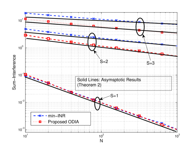
Figure 2: Normalized sum-interference vs. $N$ when $K=3$, $M=4$, $L=2$.

To evaluate the sum-rates of the proposed ODIA schemes, the parameters $\eta_{I}$, $\eta_{D}$, and $\alpha$ need to be optimized for the SE-ODIA. Fig. 3 shows the sum-rate performance of the proposed SE-ODIA for varying $\eta_{I}$ or $\eta_{D}$ with two different $\alpha$ values when $K=3$, $M=4$, $L=2$, $S=2$, and $N=20$. To obtain the sum-rate according to $\eta_{I}$, $\eta_{D}$ was fixed to $1$. Similarly, for the sum-rate according to $\eta_{D}$, $\eta_{I}$ was fixed to $1$. If $\eta_{I}$ is too small, then there may not be eligible users that satisfy the conditions $\mathsf{C}_{1}$ and $\mathsf{C}_{2}$ in (57). Thus, scheduling outage  can occur frequently and the achievable sum-rate becomes low. On the other hand, if $\eta_{I}$ is too large, then the received interference at users may not be sufficiently suppressed. Thus, the achievable sum-rate converges to that of the system without interference suppression. Similarly, if $\eta_{D}$ is too large, then the scheduling outage occurs; and if $\eta_{D}$ is too small, then desired channel gains cannot be improved. The orthogonality parameter $\alpha$ plays a similar role; if $\alpha$ is too small, the cardinality of the user pool $|\mathcal{N}_{s}|$ often becomes smaller than $S$, and scheduling outage happens frequently. If $\alpha$ is too large, then the orthogonality of the effective channel vectors of the selected users is not taken into account for scheduling. In short, the parameters $\eta_{I}$, $\eta_{D}$, and $\alpha$ need to be carefully chosen to improve the performance of the proposed SE-ODIA. In subsequent sum-rate simulations, proper sets of $\eta_{I}$, $\eta_{D}$, and $\alpha$ were numerically found for various $N$ and SNR values and applied to the SE-ODIA.

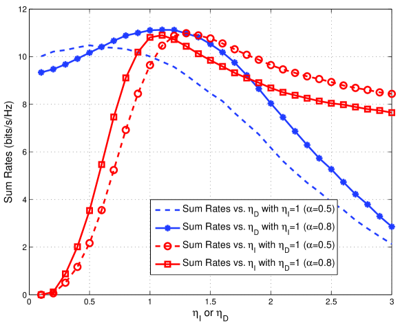
Figure 3: Sum-rates of SE-ODIA vs. $\eta_{D}$ or $\eta_{I}$ when $K=3$, $M=4$, $L=2$, $S=2$, and $N=20$.

For instance, optimal $(\eta_{I},\eta_{D},\alpha)$ values that maximize the sum-rate for a few cases are provided in Table I. It is seen that in the noise-limited low SNR regime, large $\eta_{D}$ helps, whereas in the interference-limited high SNR regime, small $\eta_{I}$ improves the sum-rate. On the other hand, as $N$ increases, interference can be suppressed by choosing smaller $\eta_{I}$ values.

TABLE I: Optimized parameters $(\eta_{I},\eta_{D},\alpha)$ for different SNRs and $N$ values

	$N$=20	$N$=50
SNR=3dB	(2.5, 2.5, 0.8)	(2, 2.5, 0.8)
SNR=21dB	(1.5, 2, 0.8)	(1, 2, 0.8)

Fig. 4 shows the sum-rates for varying SNR values when $K=3$, $M=4$, $L=2$, $S=2$, and (a) $N=20$ and (b) $N=50$. In the noise-limited low SNR regime, the sum-rate of the min-INR scheme is even lower than that of the max-SNR scheme, because $N$ is not large enough to suppress both intra- and inter-cell interference. The proposed ODIA outperforms the conventional schemes for SNRs larger than 2dB due to the combined effort of 1) transmit beamforming perfectly eliminating intra-cell interference and 2) receive beamforming effectively reducing inter-cell interference. The sum-rate performance of the ODIA with limited feedback (ODIA-LF) improves as $n_{f}$ increases as expected. In practice, $n_{f}=6$ exhibits a good compromise between the number of feedback bits and sum-rate performance for the codebook dimension of 2 (i.e., $S=2$). On the other hand, the proposed SE-ODIA achieves higher sum-rates than the others including the ODIA for all SNR regime, because the SE-ODIA improves desired channel gains and suppresses interference simultaneously. Note however that the SE-ODIA includes the optimization on the parameters for given SNR and $N$ and requires the user scheduling method based on perfect CSI feedback, which demands higher computational complexity than the user scheduling of the ODIA. As shown in Fig. 4, the amount of sum-rates improvement of the proposed ODIA schems for growing $N$ is much larger than those of the conventional schemes.

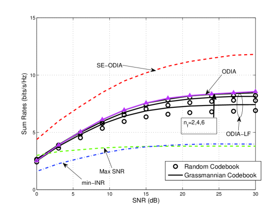
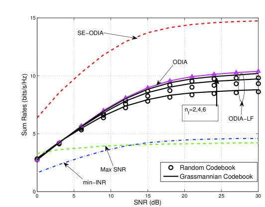
Figure 4: Sum-rates versus SNR when $K=3$, $M=4$, $L=2$, $S=2$, and (a) $N=20$ (b) $N=50$.

Fig. 5 shows the sum-rate performance of the proposed ODIA schemes for varying number of users per cell, $N$, when $K=3$, $M=4$, $L=2$, $S=2$, and SNR=$20$dB. For limited feedback, the Grassmannian codebook was employed. The sum-rates of the proposed ODIA schemes increase faster than the two conventional schemes, which implies that the user scaling conditions of the proposed ODIA schemes required for a given DoF or MUD gain are lowered than the conventional schemes, as shown in Theorems 1 and 4.

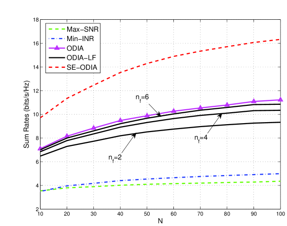
Figure 5: Sum-rates vs. $N$ when $K=3$, $M=4$, $L=2$, $S=2$, and SNR=20dB.

VIII Conclusion

In this paper, we proposed an opportunistic downlink interference alignment (ODIA) which intelligently combines user scheduling, transmit beamforming, and receive beamforming for multi-cell downlink networks. In the ODIA, the optimal DoF can be achieved with more relaxed user scaling condition $N=\left(\mathsf{SNR}^{(K-1)L-S+1}\right)$. To the best of our knowledge, this user scaling condition is the best known to date. We also considered a limited feedback approach for the ODIA, and analyzed the minimum number of feedback bits required to achieve the same user scaling condition of the ODIA with perfect feedback. We found that both Grassmannian and random codebooks yield the same condition on the number of required feedback bits. Finally, a spectrally efficient ODIA (SE-ODIA) was proposed to further improve the sum-rate of the ODIA, in which optimal multiuser diversity can be achieved even in the presence of inter-cell interference. Through numerical results, it was shown that the proposed ODIA schemes significantly outperform the conventional interference management schemes in practical environments.

Appendix A Proof of Lemma 2

Recall that the selected users’ $\eta^{[i,j]}$ are the minimum $S$ values out of $N$ i.i.d. random variables. For given $S$, suppose the worse performance case where $N$ users are randomly divided into $S$ subgroups with $N/S$ users per each and where one user with the minimum $\eta^{[i,j]}$ is selected for each subgroup. Thus, $\eta^{[i,j]}$ is the minimum of $N/S$ i.i.d. random variables. At this point, let us define $\beta$ such that

$$\textrm{Pr}\left\{\eta^{[i,j]}\leq\frac{1}{\beta}\right\}=\frac{S}{N}.$$ (78)

Note that since $\eta^{[i,j]}$ only decreases with respect to $N$, $\beta$ also decreases as $N$ increases from (78). In addition, since the CDF of $\eta^{[i,j]}$ obtained from (22) is the same as that of the scheduling metric of the MIMO IMAC [14], the CDF of $\eta^{[i,j]}$ is given by [14, Lemma 1]

$$F_{\eta}(x)=c_{0}x^{(K-1)S-L+1}+o\left(x^{(K-1)S-L+1}\right),$$ (79)

where $c_{0}$ is a constant determined by $K$, $S$, and $L$. Thus, we have $\textrm{Pr}\left\{\eta^{[i,j]}\leq\frac{1}{\beta}\right\}=c_{0}\beta^{-\tau}+o\left(\beta^{-\tau}\right)$ from Lemma 1, where $\tau=(K-1)S-L+1$, and hence $\beta=\Theta\left(N^{1/\tau}\right)$. In addition, since selected user’s $1/\eta^{[i,j]}$ is the maximum out of $N/S$ reversed scheduling metrics, it can be shown from (78) that

$$\textrm{Pr}\left\{\frac{1}{\eta^{[i,j]}|_{\textrm{selected}}}\leq\beta\right\} =\left(1-\frac{1}{N/S}\right)^{N/S}.$$ (80)

Therefore, the Markov inequality yields

$$E\left\{\frac{1}{\eta^{[i,j]}|_{\textrm{selected}}}\right\} \geq\beta\cdot\textrm{Pr}\left\{\frac{1}{\eta^{[i,j]}|_{\textrm{selected}}}\geq\beta\right\}$$ (81)

$$=\beta\cdot\left(1-\left(1-\frac{1}{N/S}\right)^{N/S}\right)$$ (82)

$$=\Theta\left(N^{1/\tau}\right),$$ (83)

where (83) follows from the fact that $\beta=\Theta\left(N^{1/\tau}\right)$ and $\left(1-\frac{1}{N/S}\right)^{N/S}$ converges to a constant for increasing $N$.

Appendix B Proof of Theorem 3

i) Grassmannian codebook
For the Grassmannian codebook, the chordal distance between any two codewords is the same, i.e., $\sqrt{1-\left|\mathbf{c}_{i}^{\mathsf{H}}\mathbf{c}_{j}\right|^{2}}=d,$, $\forall i\neq j$. The Rankin, Gilbert-Varshamov, and Hamming bounds on the chordal distance give us [32, 33, 34]

$${d^{[i,j]}}^{2}\leq\operatornamewithlimits{min}\left\{\frac{1}{2},\frac{(S-1)N_{f}}{2S(N_{f}-1)},\left(\frac{1}{N_{f}}\right)^{1/(S-1)}\right\}.$$ (84)

The bound in (84) is reduced to the third bound as $N_{f}$ increases, thus providing arbitrarily tight upper-bound on ${d^{[i,j]}}^{2}$. Thus, the first term of (47) remains constant if

$$\left(d^{\operatorname{max}}_{i}\right)^{2}\delta_{1}\cdot\mathsf{SNR} \leq\left(\frac{1}{N_{f}}\right)^{1/(S-1)}\delta_{1}\cdot\mathsf{SNR}\leq\epsilon^{\prime}.$$ (85)

This is reduced to $N_{f}^{-1/(S-1)}\leq\epsilon^{\prime}\delta_{1}^{-1}\mathsf{SNR}^{-1}$, or equivalently (37). Now, if (37) holds true, $d_{i}^{\operatorname{max}}$ tends to be arbitrarily small as SNR increases, and thus the second term of (47) is dominated by the first term. Therefore, if $n_{f}$ scales with respect to $\operatorname{log}_{2}(\mathsf{SNR})$ as (37), the residual intra-cell interference $\Delta^{[i,j]}$ remains constant.

ii) Random codebook
In a random codebook, each codeword $\mathbf{c}_{k}$ is chosen isotropically and independently from the $L$-dimensional hyper sphere, and thus the maximum chordal distance of a random codebook is unbounded. Since ${d^{[i,j]}}^{2}$ is the minimum of $N_{f}$ chordal distances resulting from $N_{f}$ independent codewords, the CDF of ${d^{[i,j]}}^{2}$ is given by [35, 21]

$$F_{d}(z)\triangleq\textrm{Pr}\left\{{d^{[i,j]}}^{2}\leq z\right\}=1-\left(1-z^{S-1}\right)^{N_{f}}.$$ (86)

From (47), the second term of (V) can be bounded by

$$\textrm{Pr}\Bigg{\{}\Delta^{[i,j]}\leq\epsilon^{\prime},\forall i\in\mathcal{K},j\in\mathcal{S}\Bigg{\}}$$

$$\hskip 10.0pt\geq\textrm{Pr}\left\{\left(d^{\operatorname{max}}_{i}\right)^{2}\delta_{1}\cdot\mathsf{SNR}\leq\epsilon^{\prime},\forall i\in\mathcal{K}\right\}$$

$$\hskip 30.0pt\times\textrm{Pr}\left\{\sum_{k=2}^{\infty}\left(d^{\operatorname{max}}_{i}\right)^{2k}\delta_{k}\cdot\mathsf{SNR}\leq\epsilon^{\prime},\forall i\in\mathcal{K}\right\}.$$ (87)

Subsequently, we have

$$\textrm{Pr}\left\{\left(d^{\operatorname{max}}_{i}\right)^{2}\delta_{1}\cdot\mathsf{SNR}\leq\epsilon^{\prime}\right\}=\prod_{k=1}^{S}\textrm{Pr}\left\{\left(d^{[k,i]}\right)^{2}\delta_{1}\cdot\mathsf{SNR}\leq\epsilon^{\prime}\right\},$$ (88)

which follows from the fact that $d^{[k,i]}$ and $d^{[m,i]}$ are independent for $k\neq m$. From (86) we have

$$\textrm{Pr}\left\{\left(d^{[k,i]}\right)^{2}\delta_{1}\cdot\mathsf{SNR}\leq\epsilon^{\prime}\right\}$$

$$\hskip 20.0pt=1-\left(1-{\epsilon^{\prime}}^{S-1}\delta_{1}^{-S+1}\left(\mathsf{SNR}\right)^{-(S-1)}\right)^{N_{f}}.$$ (89)

Therefore, $\lim_{\mathsf{SNR}\rightarrow\infty}\textrm{Pr}\left\{\left(d^{\operatorname{max}}_{i}\right)^{2}\delta_{1}\cdot\mathsf{SNR}\leq\epsilon^{\prime}\right\}=1$ if and only if $N_{f}=\omega\left(\mathsf{SNR}^{S-1}\right)$, or equivalently (37). Now, if (37) holds true, $d_{i}^{\operatorname{max}}$ tends to arbitrarily small with high probability as SNR increases. Therefore, the second term of (47) is dominated by the first term, and hence $\textrm{Pr}\left\{\Delta^{[i,j]}\leq\epsilon^{\prime},\forall i\in\mathcal{K},j\in\mathcal{S}\right\}$ in (B) tends to 1.

Appendix C Proof of Lemma 3

Let us define the set $\Pi_{s}$ by

$$\Pi_{s}\triangleq\left\{\mathbf{h}\in\mathbb{C}^{S\times 1}:\frac{{\mathbf{h}}^{\mathsf{H}}\mathbf{v}}{\|\mathbf{h}\|\|\mathbf{v}\|}<\alpha,\forall\mathbf{v}\in\textrm{span}\left(\mathbf{b}_{1}^{[i]},\ldots,\mathbf{b}_{s-1}^{[i]}\right)\right\}.$$ (90)

Since the $s$-th user pool is determined only by checking the orthogonality to the chosen users’ channel vectors, for arbitrarily large $N$, we have the followings by the law of large numbers:

$$|\mathcal{N}_{s}| \approx N\cdot\textrm{Pr}\left\{\mathbf{h}\in\mathbb{C}^{S\times 1}:\frac{{\mathbf{h}}^{\mathsf{H}}{\mathbf{b}_{s}^{[i]}}^{\prime}}{\|\mathbf{h}\|\|\mathbf{b}_{s^{\prime}}^{[i]}\|}<\alpha,s^{\prime}=1,\ldots,s-1\right\}$$ (91)

$$\geq N\cdot\textrm{Pr}\left\{\mathbf{h}\in\mathbb{C}^{S\times 1}:\mathbf{h}\in\Pi_{s}\right\}$$ (92)

$$=N\cdot I_{\alpha^{2}}(s-1,S-s+1)$$ (93)

$$\geq N\cdot\alpha^{2(S-1)},$$ (94)

where $I_{\alpha^{2}}$ is the regularized incomplete beta function (See [30, Lemma 3]), and (94) follows from $I_{\alpha^{2}}(s-1,S-s+1)\geq I_{\alpha^{2}}(S-1,1)=\alpha^{2(S-1)}$.

Appendix D Proof of (71)

Since $\left\|\mathbf{b}_{s}^{[i]}\right\|^{2}$ is a Chi-squared random variable with $2(S-s+1)$ degrees-of-freedom, for $\eta_{D}>2$, we have

$$\textrm{Pr}\left\{\mathsf{C}_{2}\right\} =1-\frac{\gamma((S-s+1),\eta_{D}/2)}{\Gamma(S-s+1)}=\frac{\Gamma((S-s+1),\eta_{D}/2)}{\Gamma(S-s+1)}$$ (95)

$$=\sum_{m=0}^{S-s}e^{-(\eta_{D}/2)}\frac{{(\eta_{D}/2)}^{m}}{m!}$$ (96)

$$=\frac{e^{-(\eta_{D}/2)}\cdot{(\eta_{D}/2)}^{S-s}}{(S-s)!}\left(1+O\left({(\eta_{D}/2)}^{-1}\right)\right)$$ (97)

$$\geq\frac{e^{-(\eta_{D}/2)}}{(S-s)!},$$ (98)

where $\Gamma(s,x)=\int_{x}^{\infty}t^{s-1}e^{-t}dt$ is the upper incomplete gamma function and $\gamma(s,x)=\int_{0}^{x}t^{s-1}e^{-t}dt$ is the lower incomplete gamma function.

Note that from the CDF of $\eta^{[i,j]}$ (See [14, Lemma 1]), $\textrm{Pr}\left\{\eta^{[i,j]}\leq\eta_{I}\right\}=c_{0}\eta_{I}^{\tau}+o(\eta_{I}^{\tau})$, where $\tau=(K-1)S-L+1$. Thus, from (64), (65), and (98), (69) can be bounded by

$$\mathsf{p}_{s} \gtrsim 1-\Bigg{(}1-\left(c_{0}(\epsilon_{I})^{\tau}{\mathsf{SNR}}^{-\tau}+\Omega\left({\mathsf{SNR}}^{-(\tau-1)}\right)\right)$$

$$\hskip 100.0pt\times\frac{N^{-(\epsilon_{D}/2)}}{(S-s)!}\Bigg{)}^{N\cdot\alpha^{2(S-1)}}.$$ (99)

The right-hand side of (D) converges to 1 for increasing SNR if and only if

$$\lim_{\mathsf{SNR}\rightarrow\infty}\left(N\cdot\alpha^{2(S-1)}\right)\cdot\left(c_{0}(\epsilon_{I})^{\tau}{\mathsf{SNR}}^{-\tau}+\Omega\left({\mathsf{SNR}}^{-(\tau-1)}\right)\right)$$

$$\hskip 50.0pt\times\frac{N^{-(\epsilon_{D}/2)}}{(S-s)!}\rightarrow\infty.$$ (100)

Since the left-hand side of (D) can be written by $\tilde{c}_{0}\frac{N^{1-(\epsilon_{D}/2)}}{\mathsf{SNR}^{\tau}}+\tilde{c}_{1}\frac{N^{1-(\epsilon_{D}/2)}}{o\left(\mathsf{SNR}^{\tau}\right)}$, where $\tilde{c}_{0}$ and $\tilde{c}_{1}$ are positive constants independent of SNR and $N$, it tends to infinity for increasing SNR, and thereby $\mathsf{p}_{s}$ tends to 1 if and only if $N=\omega\left(\mathsf{SNR}^{\frac{(K-1)S-L+1}{1-(\epsilon_{D}/2)}}\right)$.

References

• [1] V. R. Cadambe and S. A. Jafar, “Interference alignment and degrees of freedom of the K-user interference channel,” IEEE Trans. Inf. Theory, vol. 54, no. 8, pp. 3425–3441, Aug. 2008.
• [2] K. Gomadam, V. R. Cadambe, and S. A. Jafar, “A distributed numerical approach to interference alignment and applications to wireless interference networks,” IEEE Trans. Inf. Theory, vol. 57, no. 6, pp. 3309–3322, June 2011.
• [3] T. Gou and S. A. Jafar, “Degrees of freedom of the K user M X N MIMO interference channel,” IEEE Trans. Inf. Theory, vol. 56, no. 12, pp. 6040–6057, Dec. 2010.
• [4] C. Suh, M. Ho, and D. Tse, “Downlink interference alignment,” IEEE Trans. Commun., vol. 59, no. 9, pp. 2616–2626, Sept. 2011.
• [5] C. Suh and D. Tse, “Interference alignment for cellular networks,” in Proc. 46th Annual Allerton Conf. Communication, Control, and Computing, Urbana-Champaign, IL, Sept. 2008, pp. 1037 – 1044.
• [6] R. Knopp and P. Humblet, “Information capacity and power control in single cell multiuser communications,” in Proc. Int’l Conf. Commun. (ICC), Seattle, WA, June 1995, pp. 331–335.
• [7] P. Viswanath, D. N. C. Tse, and R. Laroia, “Opportunistic beamforming using dumb antennas,” IEEE Trans. Inf. Theory, vol. 48, no. 6, pp. 1277–1294, Aug. 2002.
• [8] M. Sharif and B. Hassibi, “On the capacity of MIMO broadcast channels with partial side information,” IEEE Trans. Inf. Theory, vol. 51, no. 2, pp. 506–522, Feb. 2005.
• [9] W.-Y. Shin, S.-Y. Chung, and Y. H. Lee, “Parallel opportunistic routing in wireless networks,” IEEE Trans. Inf. Theory, to appear.
• [10] T. W. Ban, W. Choi, B. C. Jung, and D. K. Sung, “Multi-user diversity in a spectrum sharing system,” IEEE Trans. Wireless Commun., vol. 8, no. 1, pp. 102–106, Jan. 2009.
• [11] W. Y. Shin, D. Park, and B. C. Jung, “Can one achieve multiuser diversity in uplink multi-cell networks?” IEEE Trans. Commun., vol. 60, no. 12, pp. 3535–3540, Dec. 2012.
• [12] B. C. Jung and W.-Y. Shin, “Opportunistic interference alignment for interference-limited cellular TDD uplink,” IEEE Commun. Lett., vol. 15, no. 2, pp. 148–150, Feb. 2011.
• [13] B. C. Jung, D. Park, and W.-Y. Shin, “Opportunistic interference mitigation achieves optimal degrees-of-freedom in wireless multi-cell uplink networks,” IEEE Trans. Commun., vol. 60, no. 7, pp. 1935–1944, July 2012.
• [14] H. J. Yang, W.-Y. Shin, B. C. Jung, and A. Paulraj, “Opportunistic interference alignment for MIMO interfering multiple access channels,” IEEE Trans. Wireless Commun., vol. 12, no. 5, pp. 2180–2192, May 2013.
• [15] W.-Y. Shin and B. C. Jung, “Network coordinated opportunistic beamforming in downlink cellular networks,,” IEICE Trans. Commun., vol. E95-B, no. 4, pp. 1393–1396, Apr. 2012.
• [16] J. Jose, S. Subramanian, X. Wu, and J. Li, “Opportunistic interference alignment in cellular downlink,” in 50th Annual Allerton Conference on Communication, Control, and Computing (Allerton), 2012, pp. 1529–1545.
• [17] J. H. Lee and W. Choi, “On the achievable dof and user scaling law of opportunistic interference alignment in 3-transmitter MIMO interference channels,” IEEE Trans. Wireless Commun., vol. 12, no. 6, pp. 2743–2753, Jun. 2013.
• [18] H. D. Nguyen, R. Zhang, and H. T. Hui, “Multi-cell random beamforming: Achievable rate and degrees-of-freedom region,” IEEE Trans. Signal Process., vol. 61, no. 14, pp. 3532–3544, July 2013.
• [19] ——, “Effect of receive spatial diversity on the degrees-of-freedom region in multi-cell random beamforming,” IEEE Trans. Wireless Commun., submitted, Preprint, [Online]. Available: http://arxiv.org/abs/1303.5947.
• [20] J. H. Lee, W. Choi, and B. D. Rao, “Multiuser diversity in interfering broadcast channels: Achievable degrees of freedom and user scaling law,” IEEE Trans. Wireless Commun., vol. 12, no. 11, pp. 5837–5849, Nov. 2013.
• [21] N. Jindal, “MIMO broadcast channels with finite-rate feedback,” IEEE Trans. Inform. Theory, vol. 52, no. 11, Nov. 2006.
• [22] T. Yoo, N. Jindal, and A. Goldsmith, “Multi-antenna downlink channels with limited feedback and user selection,” IEEE J. Select. Areas Commun., vol. 25, no. 7, pp. 1478–1491, Sept. 2007.
• [23] J. Thukral and H. Bölcskei, “Interference alignment with limited feedback,” in Proc. IEEE Int’l Symp. Inf. Theory (ISIT), Seoul, Korea, July 2009, pp. 1759–1763.
• [24] R. T. Krishnamachari and M. K. Varanasi, “Interference alignment under limited feedback for MIMO interference channels,” in Proc. IEEE Int’l Symp. Inf. Theory (ISIT), AUstin, TX, June 2010, pp. 619–623.
• [25] S. Pereira, A. Paulraj, and G. Papanicolaou, “Opportunistic scheduling for multiantenna cellular: Interference limited regime,” in Proc. Asilomar Conference on Signals, Systems and Computers, Pacific Grove, CA, Nov. 2007.
• [26] L. Choi and R. D. Murch, “A transmit preprocessing technique for multiuser MIMO systems using a decomposition approach,” IEEE Trans. Wireless Commun., vol. 3, no. 1, pp. 20–24, Jan. 2004.
• [27] D. J. Love and R. W. Heath, Jr., “Grassmannian beamforming for multiple-input multple-output wireless systems,” IEEE Trans. Inf. Theory, vol. 49, no. 10, pp. 2735–2747, Oct. 2003.
• [28] C. K. Au-Yeung and D. J. Love, “Optimization and tradeoff analysis of two-way limited feedback beamforming systems,” IEEE Trans. Wireless Commun., vol. 8, no. 5, pp. 2570–2579, May 2009.
• [29] B. Khoshnevis, “Multiple-antenna communications with limited channel state information,” Ph.D. dissertation, University of Toronto, 2011.
• [30] T. Yoo and A. Goldsmith, “On the optimality of multi-antenna broadcast scheduling using zero-forcing beamforming,” IEEE J. Select. Areas Commun., vol. 24, pp. 528–541, 2006.
• [31] G. A. F. Seber and J. L. Alan, Linear Regression Analysis, 2nd ed.   Wiley, 2003.
• [32] A. Barg and D. Y. Nogin, “Bounds on packings of spheresin the Grassmann manifold,” IEEE Trans. Inf. Theory, vol. 48, no. 9, pp. 2450–2454, Sept. 2002.
• [33] J. H. Conway, R. H. Hardin, and N. J. A. Sloane, “Packing lines, planes, etc.: Packings in Grassmannian spaces,” Experimental Mathematics, vol. 5, pp. 139–159, 1996.
• [34] W. Dai, Y. E. Liu, and B. Rider, “Quantization bounds on Grassmann manifolds and applications to MIMO communications,” IEEE Trans. Inf. Theory, vol. 54, no. 3, pp. 1108–1123, Mar. 2008.
• [35] C. K. Au-Yeung and D. J. Love, “On the performance of random vector quantization limited feedback beamforming in a MISO system,” IEEE Trans. Wireless Commun., vol. 6, no. 2, pp. 458–462, Feb. 2007.