The Ramond Sector of Heterotic String Field Theory

Abstract

We attempt to construct the full equations of motion for the Neveu-Schwarz and the Ramond sectors of the heterotic string field theory. Although they are also non-polynomial in the Ramond string field $\Psi$, we can construct them order by order in $\Psi$. Their explicit forms with the gauge transformations are given up to the next-to-next-to-leading order in $\Psi$. We also determine a subset of the terms to all orders. By introducing an auxiliary Ramond string field $\Xi$, we construct a covariant action supplemented with a constraint, which should be imposed on the equations of motion. We propose the Feynman rules and show how they reproduce well-known physical four-point amplitudes with external fermions.

1 Introduction

The Neveu-Schwarz (NS) sector of the heterotic string field theory was first constructed order by order in the coupling constant using the large Hilbert space of the superghosts.[1] Soon afterwards, it was completed by giving the action and gauge transformations in a closed form as a Wess-Zumino-Witten (WZW)-like theory,[2] which is a natural extension of the similar formulation of the open superstring field theory[3]. This heterotic string field theory is a closed string field theory with non-polynomial interactions (in the NS string field), which can be constructed based on the polyhedral overlapping conditions.[4, 5, 6, 7, 8, 9] The corresponding string products satisfy a set of identities with an additional derivation $\eta$ characterizing the algebraic structure of the heterotic string field theory. An analog of the Maurer-Cartan form, the basic ingredient of the WZW-like action, can be constructed by means of the pure gauge field in bosonic closed string field theory.[2]

On the other hand, the Ramond (R) sector of the heterotic string field theory has not been studied so far. This is presumably because one of the main motivations to construct string field theories is to find classical solutions, including the solution for tachyon condensation, which does not require the R sector. Nevertheless, it is important to understand the R sector for many other purposes, such as discussing non-renormalization theorems, supersymmetry breaking, and so on. The aim of this paper is to attempt to construct the full heterotic string field theory by including the R sector.

In the case of the WZW-like open superstring field theory, however, it was not straightforward to construct the covariant R action due to the picture number mismatch. Therefore, at first, only the equations of motion could be given in the covariant form.[10] Subsequently, a covariant action was constructed by introducing an auxiliary R string field with a constraint.[11] The auxiliary string field is eliminated by the constraint, and the equations of motion reduce to those previously obtained. According to this open superstring case, we will at first attempt to construct the equations of motion for the NS and the R sectors of the heterotic string field theory since the picture number difficulty is common to the heterotic string case.

From simple consideration, one can easily notice that the full equations of motion in the heterotic string field theory have to be non-polynomial not only in the NS string field but also in the R string field to reproduce correct fermion amplitudes. We will construct them order by order in the R string field $\Psi$ by imposing some consistency conditions, including invariance under a gauge transformation. Their explicit forms will be given up to the next-to-next-to-leading order corrections in $\Psi$. The non-polynomial gauge transformations will also be determined up to the same order. In addition, we will find a subset of terms in the equations of motion and the gauge transformations built with one or two string products to all orders.

Then we will introduce an auxiliary R string field and construct an action. The above equations of motion can be obtained from those derived from the action by eliminating the auxiliary field using a constraint,[11] which is also non-polynomial in $\Psi$. We will also propose the Feynman rules to compute tree amplitudes. Since the action has to be supplemented by the constraint, these Feynman rules cannot be simply derived by the conventional method. Nevertheless, we can extend the rules proposed for the open superstring[11] to those of the heterotic string with a few additional prescriptions. As evidence that these Feynman rules work well, we will show that they actually reproduce on-shell four-point amplitudes with external fermions.

This paper is organized as follows. In §2, we will briefly summarize the known results on the NS sector of the heterotic string field theory. The heterotic string fields are defined based on the large Hilbert space of superghosts for the holomorphic, superstring, sector. Together with the NS string field $V$, we will also introduce the R string field $\Psi$ here. After explaining the fundamental properties of the string products, the WZW-like action of the NS sector will be given. We will attempt to construct the full equations of motion, including interactions with the R sector, in §3, and find a general form of the full equations of motion required by a gauge invariance. The explicit forms of the equations of motion and the gauge transformations will be given up to the next-to-next-to-leading order in $\Psi$. We will also determine a subset of terms to all orders. We will construct, in §4, an action and a constraint by introducing an auxiliary R string field $\Xi$. In §5, we will propose the Feynman rules by adding a few prescriptions to the straightforward extensions of those for the open superstring field theory.[11] We will show how well-known four-point fermion amplitudes are reproduced. Section 6 is devoted to open questions and discussion. We add three appendices. In Appendix A, We will give the explicit forms of the gauge transformations at the next-to-next-to-leading order in $\Psi$. We will explain in detail how the general form of the full equations of motion are obtained by imposing a gauge invariance in Appendix B. The derivation of the all-order results in §3 will be presented in Appendix C. The gauge transformation laws built with two string products will also be given.

2 The NS sector of the heterotic string field theory

In this section, we summarize the known results in the NS sector of the heterotic string field theory.[1, 2]. Together with the NS string field $V$, the R string field $\Psi$ is also introduced. After introducing the string products and discussing their fundamental properties, the gauge-invariant WZW-like action is given.

2.1 Heterotic string fields

The first quantized heterotic string in a consistent background is in general described by a conformal field theory with the following structure of holomorphic and anti-holomorphic sectors. The holomorphic sector is composed of the Hilbert spaces of an $N=1$ superconformal matter with central charge $c=15$, the reparametrization ghosts $(b(z),c(z))$ with $c=-26$ and the bosonized superghosts $(\xi(z),\eta(z),\phi(z))$ with $c=11$. In particular, we adopt the large Hilbert space for the superconformal ghosts involving the zero mode $\xi_{0}$ of the field $\xi(z)$. The anti-holomorphic sector consists of a conformal matter theory with $\bar{c}=26$ and the reparametrization ghosts $(\bar{b}(\bar{z}),\bar{c}(\bar{z}))$ with $\bar{c}=-26$. The normalization of correlation function in this Hilbert space is given by

$$\langle\langle\xi e^{-\phi}c\partial c\partial^{2}c\bar{c}\bar{\partial}\bar{c}\bar{\partial}^{2}\bar{c}\rangle\rangle=2.$$ (1)

There are two sectors, the NS sector and the R sector, in the full heterotic string theory depending on the boundary conditions of the holomorphic world-sheet fermions. The states in the NS (R) sector represent space-time bosons (fermions).

Using the BRST operator $Q$, the linearized equations of motion are given by

$$Q\eta V= 0,$$ (2a)

$$Q\eta\Psi= 0,$$ (2b)

for the NS string field $V$ and the R string field $\Psi$, respectively. In this paper, we denote the zero-mode $\eta_{0}$ of the field $\eta(z)$ as $\eta$, for simplicity. Due to the nilpotency $Q^{2}=\eta^{2}=0$ and the anti-commutativity $\{Q,\eta\}=0$, these equations of motion are invariant under the gauge transformations

$$\delta V= Q\Lambda_{0}+\eta\Lambda_{1},$$ (3a)

$$\delta\Psi= Q\Lambda_{\frac{1}{2}}+\eta\Lambda_{\frac{3}{2}},$$ (3b)

where $\Lambda_{n}$ with integer (half-integer) $n$ are the gauge parameter NS (R) string fields with the picture number $n$ as shown below. The on-shell physical states obtained from these equations of motion and gauge transformations coincide with those given by the conventional BRST cohomology in the small Hilbert space.[12]

In the NS string field $V$, a physical vertex operator takes the form of

$$|V\rangle=\cdots+\xi_{0}e^{-\phi}c\bar{c}V_{A}^{(NS)}(k)|0\rangle\varphi^{A}(k)+\cdots,$$ (4)

where $V_{A}^{(NS)}$ is a general matter primary operator with conformal dimensions $(1/2,1)$. The coefficient $\varphi^{A}(k)$ represents a space-time boson field, where the space-time tensor indices are simply denoted as $A$. Since the matter vertex $V_{A}^{(NS)}$ is Grassmann odd, the NS string field $V$ is found to be Grassmann odd. We also find, from the structure of (4), that the NS string field $V$ has the ghost number $(G)$ equal to one and the picture number $(P)$ equal to zero. In summary,

$$V\ :\ \textrm{Grassmann\ odd},\ (G,P)=(1,0).$$ (5)

Similarly, a physical vertex operator in the R string field has the form

$$|\Psi\rangle=\cdots+\xi_{0}e^{-\phi/2}c\bar{c}V_{\alpha}^{(R)}(k)|0\rangle\psi^{\alpha}(k)+\cdots.$$ (6)

The matter primary operator $V_{\alpha}^{(R)}$ has conformal dimension $(5/8,1)$, whose holomorphic sector is including the matter spin operator and $\alpha$ denotes the space-time tensor-spinor indices. We can assign odd Grassmann parity to the vertex $e^{-\phi/2}V_{\alpha}^{(R)}$ after imposing the GSO projection. Taking account of the fact that the space-time fermion fields $\psi^{\alpha}(k)$ are Grassmann odd, we can read from (6) that the R string field $\Psi$ is Grassmann odd and has the ghost number one and the picture number one-half:

$$\Psi\ :\ \textrm{Grassmann\ odd},\ (G,P)=(1,\frac{1}{2}).$$ (7)

The gauge parameter string fields $\Lambda_{n}$ are found, from (3), to be Grassmann even and have $(G,P)=(0,n)$.

All the heterotic string fields and the parameters,$V$, $\Psi$, and $\Lambda_{n}$ also satisfy the subsidiary conditions for the closed string:

$$b_{0}^{-}V=L_{0}^{-}V=0,\qquad b_{0}^{-}\Psi=L_{0}^{-}\Psi=0,\qquad b_{0}^{-}\Lambda_{n}=L_{0}^{-}\Lambda_{n}=0,$$ (8)

where

$$c_{0}^{\pm}=\frac{1}{2}(c_{0}\pm\bar{c}_{0}),\qquad b_{0}^{\pm}=b_{0}\pm\bar{b}_{0},\qquad L_{0}^{\pm}=L_{0}\pm\bar{L}_{0}.$$ (9)

We also define an inner product by $\langle A,B\rangle=\langle A|c_{0}^{-}|B\rangle$, where $\langle A|$ is the BPZ conjugate state of $|A\rangle$. This inner product satisfies

$$\langle A,B\rangle= (-1)^{(A+1)(B+1)}\langle B,A\rangle,$$ (10)

$$\langle XA,B\rangle= (-1)^{A}\langle A,XB\rangle,\ \textrm{with}\ X=Q\ \textrm{or}\ \eta,$$ (11)

and is non-zero if and only if the total ghost and picture numbers are equal to four and minus one, respectively:

$$G(A)+G(B)=4,\qquad P(A)+P(B)=-1.$$ (12)

2.2 String products and identities

As in the bosonic string field theory,[8, 9] the $n$ string product $(n\geq 2)$ in the heterotic string field theory is defined by a multilinear map from $n$ string fields $\{B_{i}\}$ $(i=1,\cdots,n)$ annihilated by $b_{0}^{-}$ and $L_{0}^{-}$ to one string field $[B_{1},\cdots,B_{n}]$ also annihilated by $b_{0}^{-}$ and $L_{0}^{-}$. Each string field $B_{i}$ can either be an NS string field or an R string field. We can find that the resultant string field $[B_{1},\cdots,B_{n}]$ is an NS (R) string field if the number of the R string in $\{B_{i}\}$ is even (odd) from the cut structure of the world-sheet fermions.[13] This is also consistent with the space-time fermion number conservation. The string field $[B_{1},\cdots,B_{n}]$ has ghost and picture numbers

$$(G,P)=\left(\sum_{i=1}^{n}G_{i}-2n+3,\ \sum_{i=1}^{n}P_{i}\right),$$ (13)

where $(G_{i},P_{i})$ are those of $B_{i}$.

The BRST operator $Q$ does not act as derivation on these string products but satisfies[9]

$$0= Q[B_{1},\cdots,B_{n}]+\sum^{n}_{i=1}(-1)^{(B_{1}+\cdots+B_{i-1})}[B_{1},\cdots,QB_{i},\cdots,B_{n}]$$

$$+\sum_{\underset{l+k=n}{\{i_{l},j_{k}\}}}\sigma(i_{l},j_{k})[B_{i_{1}},\cdots,B_{i_{l}},[B_{j_{1}},\cdots,B_{j_{k}}]],$$ (14)

where $\sigma(i_{l},j_{k})$ is a sign factor defined to be the sign picked up when one rearranges the sequence $\{Q,B_{1},\cdots,B_{n}\}$ into the order $\{B_{i_{1}},\cdots,B_{i_{l}},Q,B_{j_{1}},\cdots,B_{j_{k}}\}$. These identities have exactly the same form as those of bosonic closed string field theory because they have the same structure of the anti-ghost $b$ insertion. We have three additional derivations $X=\{\eta,\delta,\partial_{t}\}$ playing important roles in the heterotic string field theory. They are graded commutative with the BRST operator $XQ=(-1)^{X}QX$ and act on the string products as derivations:

$$X[B_{1},\cdots,B_{n}]=\sum^{n}_{i=1}(-1)^{X(1+B_{1}+\cdots+B_{i-1})}[B_{1},\cdots,XB_{i},\cdots,B_{n}].$$ (15)

In addition to these fundamental BRST operator $Q$ and string products $[\cdots]$, it is useful to introduce a new BRST operator $Q_{B_{0}}$,

$$Q_{B_{0}}B\equiv\ QB+\sum^{\infty}_{m=1}\frac{\kappa^{m}}{m!}[B_{0}^{m},B],$$ (16)

and string products $[\cdots]_{B_{0}}$,

$$[B_{1},\cdots,B_{n}]_{B_{0}}\equiv\ \sum^{\infty}_{m=0}\frac{\kappa^{m}}{m!}[B_{0}^{m},B_{1},\cdots,B_{n}],$$ (17)

shifted by a Grassmann even NS string field $B_{0}$ with $(G,P)=(2,0)$. If $B_{0}$ satisfies the equation

$$\mathcal{F}(B_{0})\equiv QB_{0}+\sum_{n=2}^{\infty}\frac{\kappa^{n-1}}{n!}[B_{0}^{n}]=0,$$ (18)

the shifted BRST operator $Q_{B_{0}}$ is nilpotent and the shifted string products $[\cdots]_{B_{0}}$ satisfy the same form of identities as (14):

$$0= Q_{B_{0}}[B_{1},\cdots,B_{n}]_{B_{0}}+\sum^{n}_{i=1}(-1)^{(B_{1}+\cdots+B_{i-1})}[B_{1},\cdots,Q_{B_{0}}B_{i},\cdots,B_{n}]_{B_{0}}$$

$$+\sum_{\underset{l+k=n}{\{i_{l},j_{k}\}}}\sigma(i_{l},j_{k})[B_{i_{1}},\cdots,B_{i_{l}},[B_{j_{1}},\cdots,B_{j_{k}}]_{B_{0}}]_{B_{0}}.$$ (19)

The operators $X=\{\eta,\delta,\partial_{t}\}$ are, in contrast, neither graded commutative with $Q_{B_{0}}$ nor derivation on the shifted string products $[\cdots]_{B_{0}}$. Extra terms appear in the relations from the contribution that $X$ operates on $B_{0}$:

$$Q_{B_{0}}(XB)-(-1)^{X}X(Q_{B_{0}}B)=-\kappa[XB_{0},B]_{B_{0}},$$ (20)

$$X[B_{1},\cdots,B_{n}]_{B_{0}}=\sum_{i=1}^{n}(-1)^{X(1+B_{1}+\cdots+B_{i-1})}[B_{1},\cdots,XB_{i},\cdots,B_{n}]_{B_{0}}$$

$$\hskip 85.35826pt+(-1)^{X}\kappa[XB_{0},B_{1},\cdots,B_{n}]_{B_{0}}.$$ (21)

2.3 WZW-like action for the NS sector of the heterotic string

As in the conventional WZW theory, we introduce an extra dimension parameterized by $t\in[0,1]$. The string field $V$ is extended to the $t$-dependent one $\mathcal{V}(t)$ satisfying $\mathcal{V}(0)=0$ and $\mathcal{V}(1)=V$. The fundamental quantities to construct the action are the four string fields $B_{Q}(\mathcal{V})$ and $B_{X}(\mathcal{V})$ with $X=\{\eta,\delta,\partial_{t}\}$, which are analogs of the Maurer-Cartan form $g^{-1}dg$. The most important one $B_{Q}(\mathcal{V})$ is defined by the pure gauge field $G(\mathcal{V})$ in closed bosonic string field theory associated with a finite gauge parameter $\mathcal{V}$, which satisfies Eq. (18): $\mathcal{F}(G)=0$.[2] The remaining three, $B_{X}$, are determined so that they satisfy an analog of the Maurer-Cartan equation,

$$XB_{Q}=(-1)^{X}Q_{B_{Q}}B_{X}.$$ (22)

Although we can obtain the explicit forms of these basic quantities by solving some differential equations order by order in $\kappa$,[2] here we give only their first few terms as

$$B_{Q}(\mathcal{V})= G(\mathcal{V})$$

$$= Q\mathcal{V}+\frac{\kappa}{2}[\mathcal{V},Q\mathcal{V}]+\frac{\kappa^{2}}{3!}([\mathcal{V},(Q\mathcal{V})^{2}]+[\mathcal{V},[\mathcal{V},Q\mathcal{V}]])+\cdots,$$

$$B_{X}(\mathcal{V})= X\mathcal{V}+\frac{\kappa}{2}[\mathcal{V},X\mathcal{V}]+\frac{\kappa^{2}}{3!}(2[\mathcal{V},Q\mathcal{V},X\mathcal{V}]+[\mathcal{V},[\mathcal{V},X\mathcal{V}]])+\cdots,$$ (23)

which are enough for later use.

Using these “Maurer-Cartan forms,”the NS sector action of the heterotic string field theory is written in the form[2]

$$S_{NS}=\int^{1}_{0}dt\langle\eta B_{\partial_{t}},B_{Q}\rangle.$$ (24)

From Eq. (22), we can show that an arbitrary variation of this action can be written as

$$\delta S_{NS}=-\langle\bar{B}_{\delta},\eta\bar{B}_{Q}\rangle,$$ (25)

where the string fields with a bar denote those evaluated at $t=1$, such as $\bar{B}_{\delta}=B_{\delta}(\mathcal{V}(1))=B_{\delta}(V)$. In particular, we denote hereafter $\bar{B}_{Q}=G(V)\equiv G$, for simplicity. As a result, the equation of motion becomes

$$\eta G=0.$$ (26)

By use of (25), one can also show that the action (24) is invariant under the gauge transformations,

$$\bar{B}_{\delta}(V)=Q_{G}\Lambda_{0}+\eta\Lambda_{1},$$ (27)

which are the non-linear extensions of (3a). Here the operator $Q_{G}$ is the nilpotent BRST operator (16) shifted by the $G(V)$. One can easily find that the equation of motion (26) and gauge transformations (27) coincide with (2a) and (3a), respectively, in the lowest order in $\kappa$.

We note that the string field $\eta G(V)$ in the left-hand side of the equation of motion (26) satisfies two identities,

$$Q_{G}(\eta G)\equiv 0,$$ (28)

$$\eta(\eta G)\equiv 0,$$ (29)

following from (22) and the nilpotency $\eta^{2}=Q_{G}^{2}=0$. These identities give quite powerful constraints to determine the equations of motion in the next section.

3 Equations of motion including the R sector

The full equations of motion for the NS and the R sectors of the heterotic string field theory are non-polynomial not only in the NS string field $V$ but also in the R string field $\Psi$. In this section we find their explicit forms order by order in $\Psi$ by imposing some consistency conditions. We also determine a subset of the terms to all orders.

We start with the equation of motion for the NS sector (the NS equation of motion),

$$\eta G-\frac{\kappa}{2}[(\eta\Psi)^{2}]_{G}=0,$$ (30)

including the leading-order coupling to the R string $\Psi$. This is a straightforward extension of that of the open superstring field theory.[10] We use here the string product shifted by $G(V)$, on which the shifted BRST operator $Q_{G}$ acts as derivation. As a result, (30) becomes consistent with the identity (28) by taking

$$Q_{G}\eta\Psi=0$$ (31)

to be the equation of motion for the R sector (the R equation of motion), a non-linear extension of (2b). In contrast, (30) is not consistent with another identity (29) because $\eta$ fails to be derivation of the shifted string products. If we apply $\eta$ on the left-hand side of (30), we obtain

$$\eta\left(\eta G-\frac{\kappa}{2}[(\eta\Psi)^{2}]_{G}\right)=\frac{\kappa^{2}}{2}[\eta G,(\eta\Psi)^{2}]_{G},$$ (32)

where the right-hand side is non-zero under (30) although it is higher order in $\Psi$. This inconsistency can be improved order by order in $\Psi$ by adding the correction terms to the equations of motion.

Before looking for the next order corrections, we consider here the gauge transformations. We first note that (30) and (31) are invariant under the $\Lambda_{0}$-gauge transformation,

$$\bar{B}_{\delta_{\Lambda_{0}}}(V)=Q_{G}\Lambda_{0},\qquad\delta_{\Lambda_{0}}\Psi=0,$$ (33)

since it keeps $G(V)$ invariant:

$$\delta_{\Lambda_{0}}G(V)=Q_{G}\bar{B}_{\delta_{\Lambda_{0}}}(V)=Q_{G}(Q_{G}\Lambda_{0})=0.$$ (34)

From the leading order $\Lambda_{1}$-gauge transformation of $V$, (27), we can determine that of $\Psi$ so that the R equation of motion (31) is invariant up to higher-order terms in $\Psi$. The leading-order gauge transformation is, in total, given by

$$\bar{B}_{\delta^{(0)}_{\Lambda_{1}}}(V)=\eta\Lambda_{1},\qquad\delta^{(0)}_{\Lambda_{1}}\Psi=-\kappa[\Psi,\eta\Lambda_{1}]_{G},$$ (35)

where we explicitly indicated, as the superscript on $\delta$, the fermion number difference between before and after the transformation. In fact, the R equation of motion (31) is transformed under this transformation as

$$\delta^{(0)}_{\Lambda_{1}}(Q_{G}\eta\Psi)=-\kappa[Q_{G}\eta\Psi,\eta\Lambda_{1}]_{G}+\kappa^{2}Q_{G}\left([\eta G,\Psi,\eta\Lambda_{1}]_{G}\right),$$ (36)

where the second term is $\mathcal{O}(\Psi^{3})$ under (30). The next order correction,

$$\bar{B}_{\delta^{(2)}_{\Lambda_{1}}}(V)=-\frac{\kappa^{2}}{2}[\Psi,\eta\Psi,\eta\Lambda_{1}]_{G},$$ (37)

has to be included in the transformation of $V$ to keep the NS equation of motion (30) invariant, except for the $\mathcal{O}(\Psi^{4})$ terms, as

$$(\delta^{(0)}_{\Lambda_{1}}+\delta^{(2)}_{\Lambda_{1}})\left(\eta G-\frac{\kappa}{2}[(\eta\Psi)^{2}]_{G}\right)= -\kappa[\left(\eta G-\frac{\kappa}{2}[(\eta\Psi)^{2}]_{G}\right),\eta\Lambda_{1}]_{G}+\kappa^{2}[Q_{G}\eta\Psi,\eta\Psi,\eta\Lambda_{1}]_{G}$$

$$+\frac{\kappa^{3}}{2}[\eta G,[\Psi,\eta\Psi,\eta\Lambda_{1}]_{G}]_{G}-Q_{G}\left(\frac{\kappa^{3}}{2}[\eta G,\Psi,\eta\Psi,\eta\Lambda_{1}]_{G}\right)$$

$$-\kappa^{3}[\eta\Psi,[\eta G,\Psi,\eta\Lambda_{1}]_{G}]_{G}+\mathcal{O}(\Psi^{4}).$$ (38)

The leading-order $\Lambda_{\frac{1}{2}}$-gauge transformation can similarly be determined as

$$\bar{B}_{\delta^{(0)}_{\Lambda_{1/2}}}(V)=0,\qquad\delta^{(0)}_{\Lambda_{1/2}}\Psi=Q_{G}\Lambda_{\frac{1}{2}},$$ (39)

so that the R equation of motion (31) is invariant:

$$\delta^{(0)}_{\Lambda_{1/2}}(Q_{G}\eta\Psi)=-\kappa[\eta G,Q_{G}\Lambda_{\frac{1}{2}}]_{G}.$$ (40)

The right-hand side is equal to zero except for $\mathcal{O}(\Psi^{3})$ terms under (30). The invariance of the NS equation of motion (30) requires the next order correction

$$\bar{B}_{\delta^{(2)}_{\Lambda_{1/2}}}(V)=\kappa[\eta\Psi,\Lambda_{\frac{1}{2}}]_{G}.$$ (41)

Then,

$$(\delta^{(0)}_{\Lambda_{1/2}}+\delta^{(2)}_{\Lambda_{1/2}})\left(\eta G-\frac{\kappa}{2}[(\eta\Psi)^{2}]_{G}\right)= \kappa^{2}[\left(\eta G-\frac{\kappa}{2}[(\eta\Psi)^{2}]_{G}\right),\eta\Psi,Q_{G}\Lambda_{\frac{1}{2}}]_{G}$$

$$-\eta\left(\kappa[Q_{G}\eta\Psi,\Lambda_{\frac{1}{2}}]_{G}\right)+\mathcal{O}(\Psi^{4}).$$ (42)

The invariance under the leading-order $\Lambda_{\frac{3}{2}}$-gauge transformation,

$$\bar{B}_{\delta^{(2)}_{\Lambda_{3/2}}}(V)=0,\qquad\delta^{(0)}_{\Lambda_{3/2}}\Psi=\eta\Lambda_{\frac{3}{2}},$$ (43)

is exact in this order since $\Psi$ appears only in the form of $\eta\Psi$ so far.

In order to consider further corrections, we assume that the $\Lambda_{0}$-gauge transformation (33) receives no more correction and the NS string field $V$ only appears in the correction terms through $G(V)$ in the quantities $Q_{G}$ and $[\cdots]_{G}$, which keeps the equations of motion invariant under (33). We call this assumption the G-ansatz in this paper. Then the consistency with the identity (28) requires the full equations of motion to be in the form of

$$\eta G-\frac{\kappa}{2}[\Omega^{2}]_{G}+Q_{G}\Sigma= 0,$$ (44a)

$$Q_{G}\Omega= 0,$$ (44b)

as explained in detail in Appendix B, where the string fields $\Omega$ and the $\Sigma$ have $(G,P)=(2,-1/2)$ and $(2,-1)$, respectively, and can be expanded in $\Psi$ as

$$\Omega=\sum_{n=0}^{\infty}\Omega^{(2n+1)},\qquad\Sigma=\sum_{n=0}^{\infty}\Sigma^{(2n+2)},$$ (45)

with the leading terms

$$\Omega^{(1)}=\eta\Psi,\qquad\Sigma^{(2)}=0.$$ (46)

The number in the parentheses of the superscript denotes the fermion number, that is the number of $\Psi$, of the terms included. One can see, by counting the ghost and the picture numbers using (13), that the fundamental possible terms in the $\Omega^{(2n+1)}$ and the $\Sigma^{(2n+2)}$ at each order $n\ (\geq 1)$ take the form,

$$\kappa^{2n+\alpha}[\Psi,(Q_{G}\Psi)^{k_{1}},(\eta\Psi)^{l_{1}},[\Psi,(Q_{G}\Psi)^{k_{2}},(\eta\Psi)^{l_{2}},[\cdots,[\Psi,(Q_{G}\Psi)^{k_{m}},(\eta\Psi)^{l_{m}}]_{G}\cdots]_{G}]_{G}]_{G},$$ (47)

under the G-ansatz, with $\alpha=0$ $(1)$ for $\Omega^{(2n+1)}$ $(\Sigma^{(2n+2)})$. Each term is made by use of $m$ ($1\leq m\leq n$) string products with the non-negative integers $k_{i}$ and $l_{i}$ $(1\leq i\leq m)$ restricted by the equations, $\sum_{i=1}^{m}k_{i}=n-m$, $\sum_{i=1}^{m}l_{i}=n+1+\alpha$ and $k_{m}+l_{m}\neq 0$. More general possible terms, appearing for ($n\geq 3$), can be obtained by replacing the $\eta\Psi$s in these fundamental terms with fundamental terms in $\Omega$, such as

$$\kappa^{2n+\alpha}[\Psi, (Q_{G}\Psi)^{k_{1}},(\eta\Psi)^{l_{1}-3},\Omega_{1}^{(2n_{1}+1)},(\Omega_{2}^{(2n_{2}+1)})^{2},$$

$$\times[\Psi,(Q_{G}\Psi)^{k_{2}},(\eta\Psi)^{l_{2}-1},\Omega_{3}^{(2n_{3}+1)},[\cdots,[\Psi,(Q_{G}\Psi)^{k_{m}},(\eta\Psi)^{l_{m}}]_{G}\cdots]_{G}]_{G}]_{G},$$ (48)

with $\sum_{i=1}^{m}k_{i}=n-n_{1}-2n_{2}-n_{3}-m$, $\sum_{i=1}^{m}l_{i}=n-n_{1}-2n_{2}-n_{3}+1+\alpha$ and $k_{m}+l_{m}\neq 0$, where

$$\Omega_{1}^{(2n_{1}+1)}= \kappa^{2n_{1}}[\Psi,(Q_{G}\Psi)^{k_{11}},(\eta\Psi)^{l_{11}},[\Psi,(Q_{G}\Psi)^{k_{12}},(\eta\Psi)^{l_{12}},$$

$$\hskip 85.35826pt\times[\cdots,[\Psi,(Q_{G}\Psi)^{k_{1m_{1}}},(\eta\Psi)^{l_{1m_{1}}}]_{G}\cdots]_{G}]_{G}]_{G},$$ (49)

$$\Omega_{2}^{(2n_{2}+1)}= \kappa^{2n_{2}}[\Psi,(Q_{G}\Psi)^{k_{21}},(\eta\Psi)^{l_{21}},[\Psi,(Q_{G}\Psi)^{k_{22}},(\eta\Psi)^{l_{22}},$$

$$\hskip 85.35826pt\times[\cdots,[\Psi,(Q_{G}\Psi)^{k_{2m_{2}}},(\eta\Psi)^{l_{2m_{2}}}]_{G}\cdots]_{G}]_{G}]_{G},$$ (50)

$$\Omega_{3}^{(2n_{3}+1)}= \kappa^{2n_{3}}[\Psi,(Q_{G}\Psi)^{k_{31}},(\eta\Psi)^{l_{31}},[\Psi,(Q_{G}\Psi)^{k_{32}},(\eta\Psi)^{l_{32}},$$

$$\hskip 85.35826pt\times[\cdots,[\Psi,(Q_{G}\Psi)^{k_{3m_{3}}},(\eta\Psi)^{l_{3m_{3}}}]_{G}\cdots]_{G}]_{G}]_{G},$$ (51)

with $\sum_{j=1}^{m_{i}}k_{ij}=n_{i}-m_{i}$, $\sum_{j=1}^{m_{i}}l_{ij}=n_{i}+1$ and $k_{im}+l_{im}\neq 0$ for $i=1,2,3$. Moreover, the terms obtained by moving the positions of $\eta\Psi$s are also allowed. For example, the terms

$$[\Psi,\eta\Psi,[\Psi,\eta\Psi]_{G},[\Psi,(\eta\Psi)^{2}]_{G}]_{G},\quad[\Psi,[\Psi,\eta\Psi]_{G},[\Psi,(\eta\Psi)^{3}]_{G}]_{G},\quad[\Psi,(\eta\Psi)^{2},[\Psi,\eta\Psi]_{G},[\Psi,\eta\Psi]_{G}]_{G}$$ (52)

are also possible in $\Omega^{(7)}$, which are obtained by moving $\eta\Psi$s in a term

$$[\Psi,(\Omega^{(3)})^{2}]_{G}\sim[\Psi,[\Psi,(\eta\Psi)^{2}]_{G},[\Psi,(\eta\Psi)^{2}]_{G}]_{G}.$$ (53)

After these replacements and moves, we can again replace the $\eta\Psi$s with fundamental terms in $\Omega$ and move the $\eta\Psi$s for higher $n$. All the possible terms are obtained by repeating these replacements and moves as many times as possible for given $n$.

From these general considerations, we can find that the possible next-to-leading-order corrections to the equations of motion are given by

$$\Omega^{(3)}=-\frac{\kappa^{2}}{3!}[\Psi,(\eta\Psi)^{2}]_{G},\qquad\Sigma^{(4)}=\frac{\kappa^{3}}{4!}[\Psi,(\eta\Psi)^{3}]_{G},$$ (54)

where the numerical coefficients were fixed by solving the consistency equation,

$$\eta\left(\frac{\kappa}{2}[\Omega^{2}]_{G}-Q_{G}\Sigma\right)=0,$$ (55)

with the identity (29).

As in the case of the leading order, we can obtain the gauge transformations in the next-to-leading order, $\delta^{(2)}\Psi$ and $\bar{B}_{\delta^{(4)}}$, by imposing the invariance of the R and the NS equations of motion, respectively. The results are

$$\bar{B}_{\delta^{(4)}_{\Lambda_{1}}}(V)= -\frac{\kappa^{4}}{4!}[\Psi,Q_{G}\Psi,(\eta\Psi)^{2},\eta\Lambda_{1}]_{G}-\frac{\kappa^{4}}{8}[[\Psi,\eta\Psi]_{G},\Psi,\eta\Psi,\eta\Lambda_{1}]_{G}$$

$$+\frac{\kappa^{4}}{4!}[[\Psi,(\eta\Psi)^{2}]_{G},\Psi,\eta\Lambda_{1}]_{G}+\frac{\kappa^{4}}{4!}[\Psi,[\Psi,(\eta\Psi)^{2},\eta\Lambda_{1}]_{G}]_{G}$$

$$+\frac{\kappa^{4}}{8}[\Psi,\eta\Psi,[\Psi,\eta\Psi,\eta\Lambda_{1}]_{G}]_{G},$$

$$\delta^{(2)}_{\Lambda_{1}}\Psi= -\frac{\kappa^{3}}{3!}[\Psi,Q_{G}\Psi,\eta\Psi,\eta\Lambda_{1}]_{G}-\frac{\kappa^{3}}{3}[[\Psi,\eta\Psi]_{G},\Psi,\eta\Lambda_{1}]_{G}$$

$$+\frac{\kappa^{3}}{3!}[\Psi,[\Psi,\eta\Psi,\eta\Lambda_{1}]_{G}]_{G},$$ (56)

for $\Lambda_{1}$-transformation,

$$\bar{B}_{\delta^{(4)}_{\Lambda_{1/2}}}(V)= \frac{\kappa^{3}}{8}[\Psi,(\eta\Psi)^{2},Q_{G}\Lambda_{\frac{1}{2}}]_{G}-\frac{\kappa^{3}}{3!}[[\Psi,(\eta\Psi)^{2}]_{G},\Lambda_{\frac{1}{2}}]_{G},$$

$$\delta^{(2)}_{\Lambda_{1/2}}\Psi= \frac{\kappa^{2}}{3}[\Psi,\eta\Psi,Q_{G}\Lambda_{\frac{1}{2}}]_{G},$$ (57)

for $\Lambda_{1/2}$-transformation and

$$\bar{B}_{\delta^{(4)}_{\Lambda_{3/2}}}(V)=-\frac{\kappa^{3}}{4!}[\Psi,(\eta\Psi)^{2},\eta\Lambda_{\frac{3}{2}}]_{G},\qquad\delta^{(2)}_{\Lambda_{3/2}}\Psi=-\frac{\kappa^{2}}{3!}[\Psi,\eta\Psi,\eta\Lambda_{\frac{3}{2}}]_{G},$$ (58)

for $\Lambda_{3/2}$-transformation.

The next-to-next-to-leading corrections the $\Omega^{(5)}$ and the $\Sigma^{(6)}$ are further determined by solving (55) as

$$\Omega^{(5)}= -\frac{\kappa^{4}}{5!}[\Psi,Q_{G}\Psi,(\eta\Psi)^{3}]_{G}+\frac{\kappa^{4}}{5!}[\Psi,[\Psi,(\eta\Psi)^{3}]_{G}]_{G}+\frac{4}{5!}\kappa^{4}[\Psi,\eta\Psi,[\Psi,(\eta\Psi)^{2}]_{G}]_{G}$$

$$-\frac{4}{5!}\kappa^{4}[\Psi,(\eta\Psi)^{2},[\Psi,\eta\Psi]_{G}]_{G},$$

$$\Sigma^{(6)}= \frac{\kappa^{5}}{6!}[\Psi,Q_{G}\Psi,(\eta\Psi)^{4}]_{G}-\frac{\kappa^{5}}{6!}[\Psi,[\Psi,(\eta\Psi)^{4}]_{G}]_{G}-\frac{5}{6!}\kappa^{5}[\Psi,\eta\Psi,[\Psi,(\eta\Psi)^{3}]_{G}]_{G}$$

$$-\frac{10}{6!}\kappa^{5}[\Psi,(\eta\Psi)^{2},[\Psi,(\eta\Psi)^{2}]_{G}]_{G}+\frac{5}{6!}\kappa^{5}[\Psi,(\eta\Psi)^{3},[\Psi,\eta\Psi]_{G}]_{G}.$$ (59)

The gauge transformations $\bar{B}_{\delta^{(6)}}$ and $\delta^{(4)}\Psi$ are also obtained similarly and their explicit forms are given in Appendix A since they are lengthy.

In general, we conjecture that the full equations of motion can be constructed order by order in $\Psi$ in a similar manner. In order to show that this is actually the case, we have to prove the existence of a non-trivial, but not necessarily unique, solution to the consistency equation (55). If it has a unique solution, we can, in principle, obtained the full equations of motion and also the gauge transformations in any order in $\Psi$ in the same way as above. If a non-trivial solution exists but is not unique, we must take into account the further gauge invariance(s) to find the full equations of motion, where the equations of motion and the gauge transformation(s) have to be determined simultaneously.

While we have not explicitly found all the terms of the full equations of motion, we have completely determined a subset of the terms built with one string product in the $\Omega$ and the $\Sigma$ and those with two string products in the $\Sigma$ to all orders in $\Psi$ similarly by solving (55). The result is

$$\Omega= \eta\Psi\ -\ \sum_{n=1}^{\infty}\frac{\kappa^{2n}}{(2n+1)!}[\Psi,(Q_{G}\Psi)^{n-1},(\eta\Psi)^{n+1}]_{G}+\cdots,$$ (60a)

$$\Sigma= \sum_{n=1}^{\infty}\frac{\kappa^{2n+1}}{(2n+2)!}[\Psi,(Q_{G}\Psi)^{n-1},(\eta\Psi)^{n+2}]_{G}$$

$$+\sum_{n=2}^{\infty}\underset{(m,l)\neq(0,0)}{\sum_{m=0}^{n-2}\sum_{l=0}^{n+2}}g_{n,m,l}\kappa^{2n+1}[\Psi,(Q_{G}\Psi)^{n-m-2},(\eta\Psi)^{n-l+2},[\Psi,(Q_{G}\Psi)^{m},(\eta\Psi)^{l}]_{G}]_{G}+\cdots,$$ (60b)

with

$$g_{n,m,l}=\begin{cases}\displaystyle\sum_{k=0}^{l}\left(\begin{array}[]{c}n-1\\ m+l+1-k\end{array}\right)\left(\begin{array}[]{c}n+3\\ k\end{array}\right)\frac{1}{(2n+2)!}&\textrm{for}\ (0\leq l\leq m+1),\\ \displaystyle-\sum_{k=0}^{m}\left(\begin{array}[]{c}n-1\\ k\end{array}\right)\left(\begin{array}[]{c}n+3\\ m+l+1-k\end{array}\right)\frac{1}{(2n+2)!}&\textrm{for}\ (m+2\leq l\leq n+2).\end{cases}$$ (61)

The dots in the right-hand side of (60) represent the terms built with more string products and $(\begin{smallmatrix}n\\ m\end{smallmatrix})$ is the binomial coefficient defined by

$$\left(\begin{array}[]{c}n\\ m\end{array}\right)=\begin{cases}\displaystyle\frac{n!}{(n-m)!m!}&\textrm{for}\ (0\leq m\leq n),\\ \ 0&\textrm{for}\ (m<0,\ \textrm{or}\ \ m>n).\end{cases}$$ (62)

The derivation of (60) is presented in more detail in Appendix C. The gauge transformations in the corresponding approximation are also found in a similar way to those in the fermion expansions as

$$\bar{B}_{\delta_{\Lambda_{1}}}(V)=\eta\Lambda_{1}-\sum_{n=1}^{\infty}\frac{\kappa^{2n}}{(2n)!}[\Psi,(Q_{G}\Psi)^{n-1},(\eta\Psi)^{n},\eta\Lambda_{1}]_{G}+\bar{B}^{[2]}_{\delta_{\Lambda_{1}}}(V)+\cdots,$$

$$\delta_{\Lambda_{1}}\Psi=-\sum_{n=0}^{\infty}\frac{\kappa^{2n+1}}{(2n+1)!}[\Psi,(Q_{G}\Psi)^{n},(\eta\Psi)^{n},\eta\Lambda_{1}]_{G}+\cdots,$$ (63)

$$\bar{B}_{\delta_{\Lambda_{1/2}}}(V)=\kappa[\eta\Psi,\Lambda_{\frac{1}{2}}]_{G}+\sum_{n=1}^{\infty}\frac{(n+2)\kappa^{2n+1}}{(2n+2)!}[\Psi,(Q_{G}\Psi)^{n-1},(\eta\Psi)^{n+1},Q_{G}\Lambda_{\frac{1}{2}}]_{G}+\bar{B}^{[2]}_{\delta_{\Lambda_{1}}}(V)+\cdots,$$

$$\delta_{\Lambda_{1/2}}\Psi=Q_{G}\Lambda_{\frac{1}{2}}+\sum_{n=1}^{\infty}\frac{(n+1)\kappa^{2n}}{(2n+1)!}[\Psi,(Q_{G}\Psi)^{n-1},(\eta\Psi)^{n},Q_{G}\Lambda_{\frac{1}{2}}]_{G}+\cdots,$$ (64)

$$\bar{B}_{\delta_{\Lambda_{3/2}}}(V)=-\sum_{n=2}^{\infty}\frac{(n-1)\kappa^{2n-1}}{(2n)!}[\Psi,(Q_{G}\Psi)^{n-2},(\eta\Psi)^{n},\eta\Lambda_{\frac{3}{2}}]_{G}+\bar{B}^{[2]}_{\delta_{\Lambda_{1}}}(V)+\cdots,$$

$$\delta_{\Lambda_{3/2}}\Psi=\eta\Lambda_{\frac{3}{2}}-\sum_{n=1}^{\infty}\frac{n\kappa^{2n}}{(2n+1)!}[\Psi,(Q_{G}\Psi)^{n-1},(\eta\Psi)^{n},\eta\Lambda_{\frac{3}{2}}]_{G}+\cdots,$$ (65)

where the terms built with two string products are denoted by $\bar{B}^{[2]}_{\delta}(V)$’s and explicitly given in Appendix C. We regard these results as evidence that the consistency equation (55) actually has a non-trivial solution and we can construct the full equations of motion and gauge transformations to all orders in $\Psi$.

4 Action with constraint

As in the case of the open superstring field theory,[11] one can construct an action by introducing an auxiliary R string field $\Xi$ with a constraint. The above equations of motion can be obtained from those derived from this action after eliminating $\Xi$ using the constraint.

Let us start with the bilinear action

$$S_{R}^{(2)}=\frac{1}{2}\langle\eta\Psi,Q_{G}\Xi\rangle,$$ (66)

which is a natural extension of the action in the open superstring field theory.[11] In order for this action (66) to be non-zero, the auxiliary string field $\Xi$ must have the properties:

$$\Xi\ :\ \textrm{Grassmann\ odd},\ (G,P)=(1,-\frac{1}{2}).$$ (67)

From the action $S_{NS}+S_{R}^{(2)}$, we can derive the three equations of motion,

$$\eta G-\frac{\kappa}{2}[\eta\Psi,Q_{G}\Xi]_{G}=0,\qquad Q_{G}\eta\Psi=0,\qquad\eta Q_{G}\Xi=0,$$ (68)

which are equivalent to the equations of motion with the leading-order coupling, (30) and (31), if we impose the constraint, $Q_{G}\Xi=\eta\Psi$.

In general, the full R action is given by the infinite series

$$S_{R}=\sum_{n=1}^{\infty}S_{R}^{(2n)},$$ (69)

where $S_{R}^{(2n)}$ includes $2n$ R string fields, the $\Psi$ and the $\Xi$, in total. If we take the first three terms as (66) and

$$S_{R}^{(4)}= \frac{\kappa^{2}}{4!}\langle\eta\Psi,[\Psi,(Q_{G}\Xi)^{2}]_{G}\rangle,$$ (70)

$$S_{R}^{(6)}= \frac{\kappa^{4}}{6!}\langle\eta\Psi,[\Psi,(Q_{G}\Psi),(Q_{G}\Xi)^{3}]_{G}\rangle-\frac{2}{6!}\kappa^{4}\langle\eta\Psi,[\Psi,[\Psi,(Q_{G}\Xi)^{3}]_{G}]_{G}\rangle$$

$$+\frac{2}{6!}\kappa^{4}\langle\eta\Psi,[\Psi,(Q_{G}\Xi),[\Psi,(Q_{G}\Xi)^{2}]_{G}]_{G}\rangle+\frac{3}{6!}\kappa^{4}\langle\eta\Psi,[\Psi,(Q_{G}\Xi)^{2},[\Psi,(Q_{G}\Xi)]_{G}]_{G}\rangle,$$ (71)

the action $S_{NS}+S_{R}^{(2)}+S_{R}^{(4)}+S_{R}^{(6)}$ yields the equations of motion,

$$\eta G-\frac{\kappa}{2}[\tilde{\Omega},(Q_{G}\Xi)]_{G}+Q_{G}\tilde{\Sigma}=0,\qquad Q_{G}\tilde{\Omega}=0,\qquad\eta\Theta+\Delta=0,$$ (72)

with

$$\tilde{\Omega}= \eta\Psi-\frac{\kappa^{2}}{3!}[\Psi,\eta\Psi,(Q_{G}\Xi)]_{G}$$

$$-\frac{\kappa^{4}}{5!}[\Psi,(Q_{G}\Psi),\eta\Psi,(Q_{G}\Xi)^{2}]_{G}+\frac{\kappa^{4}}{5!}[\Psi,[\Psi,\eta\Psi,(Q_{G}\Xi)^{2}]_{G}]_{G}$$

$$-\frac{2}{3\cdot 5!}\kappa^{4}[\Psi,\eta\Psi,[\Psi,(Q_{G}\Xi)^{2}]_{G}]_{G}+\frac{4}{3\cdot 5!}\kappa^{4}[\Psi,(Q_{G}\Xi),[\Psi,\eta\Psi,(Q_{G}\Xi)]_{G}]_{G}$$

$$-\frac{2}{5!}\kappa^{4}[\Psi,\eta\Psi,(Q_{G}\Xi),[\Psi,(Q_{G}\Xi)]_{G}]_{G}-\frac{2}{5!}\kappa^{4}[\Psi,(Q_{G}\Xi)^{2},[\Psi,\eta\Psi]_{G}]_{G},$$ (73)

$$\tilde{\Sigma}= \frac{\kappa^{3}}{4!}[\Psi,\eta\Psi,(Q_{G}\Xi)^{2}]_{G}$$

$$+\frac{\kappa^{5}}{6!}[\Psi,(Q_{G}\Psi),\eta\Psi,(Q_{G}\Xi)^{3}]_{G}-\frac{\kappa^{5}}{6!}[\Psi,[\Psi,\eta\Psi,(Q_{G}\Xi)^{3}]_{G}]_{G}$$

$$-\frac{2}{6!}\kappa^{5}[\Psi,\eta\Psi,[\Psi,(Q_{G}\Xi)^{3}]_{G}]_{G}-\frac{3}{6!}\kappa^{5}[\Psi,(Q_{G}\Xi),[\Psi,\eta\Psi,(Q_{G}\Xi)^{2}]_{G}]_{G}$$

$$+\frac{2}{6!}\kappa^{5}[\Psi,\eta\Psi,(Q_{G}\Xi),[\Psi,(Q_{G}\Xi)^{2}]_{G}]_{G}-\frac{2}{6!}\kappa^{5}[\Psi,(Q_{G}\Xi)^{2},[\Psi,\eta\Psi,(Q_{G}\Xi)]_{G}]_{G}$$

$$+\frac{3}{6!}\kappa^{5}[\Psi,\eta\Psi,(Q_{G}\Xi)^{2},[\Psi,(Q_{G}\Xi)]_{G}]_{G}+\frac{2}{6!}\kappa^{5}[\Psi,(Q_{G}\Xi)^{3},[\Psi,\eta\Psi]_{G}]_{G},$$ (74)

$$\Theta= Q_{G}\Xi+\frac{\kappa^{2}}{3!}[\Psi,(Q_{G}\Xi)^{2}]_{G}$$

$$+\frac{\kappa^{4}}{5!}[\Psi,(Q_{G}\Psi),(Q_{G}\Xi)^{3}]_{G}-\frac{\kappa^{4}}{5!}[\Psi,[\Psi,(Q_{G}\Xi)^{3}]_{G}]_{G}$$

$$+\frac{\kappa^{4}}{45}[\Psi,(Q_{G}\Xi),[\Psi,(Q_{G}\Xi)^{2}]_{G}]_{G}+\frac{4}{5!}\kappa^{4}[\Psi,(Q_{G}\Xi)^{2},[\Psi,(Q_{G}\Xi)]_{G}]_{G},$$ (75)

$$\Delta= \frac{\kappa^{4}}{3\cdot 5!}[\eta\Psi,(Q_{G}\Xi),[\Psi,(Q_{G}\Xi)^{2}]_{G}]_{G}-\frac{\kappa^{4}}{3\cdot 5!}[(Q_{G}\Xi)^{2},[\Psi,\eta\Psi,(Q_{G}\Xi)]_{G}]_{G}$$

$$+\frac{\kappa^{4}}{3\cdot 5!}[\Psi,\eta\Psi,[(Q_{G}\Xi)^{3}]_{G}]_{G}-\frac{\kappa^{4}}{3\cdot 5!}[\Psi,(Q_{G}\Xi),[\eta\Psi,(Q_{G}\Xi)^{2}]_{G}]_{G}$$

$$+\frac{\kappa^{4}}{5!}[\eta\Psi,(Q_{G}\Xi)^{2},[\Psi,(Q_{G}\Xi)]_{G}]_{G}-\frac{\kappa^{4}}{5!}[(Q_{G}\Xi)^{3},[\Psi,\eta\Psi]_{G}]_{G}$$

$$+\frac{\kappa^{4}}{5!}[\Psi,\eta\Psi,(Q_{G}\Xi),[(Q_{G}\Xi)^{2}]_{G}]_{G}-\frac{\kappa^{4}}{5!}[\Psi,(Q_{G}\Xi)^{2},[\eta\Psi,(Q_{G}\Xi)]_{G}]_{G}.$$ (76)

One can show that if we impose the constraint

$$Q_{G}\Xi=\Omega,$$ (77)

these quantities become

$$\tilde{\Omega}=\Omega,\qquad\tilde{\Sigma}=\Sigma,\qquad\Theta=\eta\Psi,\qquad\Delta=0,$$ (78)

with (46), (54), and (59), and thus the equations of motion (72) reduce to those obtained in the previous section.

Although we can also consider the gauge transformations, the action $S_{NS}+S_{R}^{(2)}+S_{R}^{(4)}+S_{R}^{(6)}$ has less symmetry than the corresponding equations of motion written by the $V$ and the $\Psi$. The action is only invariant under the transformations,

$$\bar{B}_{\delta_{\Lambda_{0}}}(V)=Q_{G}\Lambda_{0},\qquad\delta\Psi=0,\qquad\delta\Xi=Q_{G}\Lambda_{-\frac{1}{2}}.$$ (79)

This symmetry enhancement (decline) also happens in the open superstring field theory,[11] but the action symmetry (79) is smaller. The gauge symmetry generated by $\Lambda_{-1/2}$ requires that the auxiliary field $\Xi$ have to take the form of $Q_{G}\Xi$ in the action.

We have also completely determined a subset of terms, built with the one string product, in the full action (69) to all orders in $\Psi$ as

$$S_{R}=\frac{1}{2}\langle\eta\Psi,Q_{G}\Xi\rangle+\sum_{n=1}^{\infty}\frac{\kappa^{2n}}{(2n+2)!}\langle\eta\Psi,[\Psi,(Q_{G}\Psi)^{n-1},(Q_{G}\Xi)^{n+1}]_{G}\rangle+\cdots.$$ (80)

This reproduces the terms with one string product in (60) by imposing the constraint (77) with (60a).

5 Feynman rules and four–point amplitudes

We propose in this section the Feynman rules to compute tree-level amplitudes in the heterotic string field theory by extending those for the open superstring.[11] We show that these rules actually reproduce the correct on-shell four-point amplitudes with external fermions.

5.1 Feynman rules for tree-level amplitudes

Let us first focus on the kinetic terms

$$S_{0}=\frac{1}{2}\langle\eta V,QV\rangle+\frac{1}{2}\langle\eta\Psi,Q\Xi\rangle,$$ (81)

in the action, which are invariant under the transformations,

$$\delta V=Q\Lambda_{0}+\eta\Lambda_{1},\qquad\delta\Psi=Q\Lambda_{\frac{1}{2}}+\eta\Lambda_{\frac{3}{2}},\qquad\delta\Xi=Q\Lambda_{-\frac{1}{2}}+\eta\Lambda^{\prime}_{\frac{1}{2}}.$$ (82)

The non-trivial point is that not all of these symmetries can be extended to those of the full action. In particular, it may be worthwhile to note that even the NS propagator cannot be derived by means of the conventional method in the heterotic string field theory since the action symmetry (79) does not include that generated by $\Lambda_{1}$.

Here we simply assume that we can “effectively” fix these symmetries (82) by the gauge conditions

$$b_{0}^{+}V=\xi_{0}V=0,\qquad b_{0}^{+}\Psi=\xi_{0}\Psi=0,\qquad b_{0}^{+}\Xi=\xi_{0}\Xi=0.$$ (83)

Then, by inverting the kinetic terms (81), the propagators in this gauge are given by

$$\overbracket{\!\!VV\!\!}\equiv \Pi_{NS}=\xi_{0}\frac{b_{0}^{+}b_{0}^{-}}{L_{0}^{+}}\delta(L_{0}^{-})=\xi_{0}b_{0}^{+}b_{0}^{-}\int_{0}^{\infty}\!\!dT\!\!\int_{0}^{2\pi}\frac{d\theta}{2\pi}e^{-TL^{+}_{0}-i\theta L^{-}_{0}},$$ (84)

$$\overbracket{\!\!\Psi\Xi\!\!}=\overbracket{\!\!\Xi\Psi\!\!}\equiv \Pi_{R}=2\xi_{0}\frac{b_{0}^{+}b_{0}^{-}}{L_{0}^{+}}\delta(L_{0}^{-})=2\Pi_{NS}.$$ (85)

As in the open superstring field theory,[11] the constraint can be taken into account by replacing the $Q\Xi$ and the $\eta\Psi$ with their self-dual part $\omega=(Q\Xi+\eta\Psi)/2$ in the vertices. However, the $\Xi$ and the $\Psi$ do not always appear in the action (69) in the form of the $Q\Xi$ and the $\eta\Psi$, respectively. Some preparation is needed in advance of the replacement.

First, we point out that the open superstring action can be written in a similar form of the heterotic string action by using the relation,

$$Q^{\prime}A=QA+[(e^{-\Phi}Qe^{\Phi}),A\}=e^{-\Phi}(Q\tilde{A})e^{\Phi},$$ (86)

with $\tilde{A}=e^{\Phi}Ae^{-\Phi}$. It is reasonable to expect that a similar relation enables us to rewrite the action (69) in the opposite direction so that the redefined auxiliary field $\tilde{\Xi}$ always appears in the form of $Q\tilde{\Xi}$. Actually, we can show, up to $\mathcal{O}(\kappa^{3})$, that the relation

$$Q_{G}\Xi= Q\tilde{\Xi}+\kappa[V,Q\tilde{\Xi}]+\frac{\kappa^{2}}{2}[V,QV,Q\tilde{\Xi}]+\frac{\kappa^{2}}{2}[V,[V,Q\tilde{\Xi}]]$$

$$+\frac{\kappa^{3}}{3!}[V,(QV)^{2},Q\tilde{\Xi}]+\frac{\kappa^{3}}{3!}[V,[V,QV,Q\tilde{\Xi}]]+\frac{\kappa^{3}}{3}[V,QV,[V,Q\tilde{\Xi}]]$$

$$+\frac{\kappa^{3}}{3!}[[V,QV],V,Q\tilde{\Xi}]+\frac{\kappa^{3}}{3!}[V,[V,[V,Q\tilde{\Xi}]]]+\cdots,$$ (87)

holds, where

$$\tilde{\Xi}= \Xi-\kappa[V,\Xi]-\frac{\kappa^{2}}{2}[V,QV,\Xi]+\frac{\kappa^{2}}{2}[V,[V,\Xi]]-\frac{\kappa^{3}}{3!}[V,(QV)^{2},\Xi]+\frac{\kappa^{3}}{3}[V,[V,QV,\Xi]]$$

$$+\frac{\kappa^{3}}{3!}[V,QV,[V,\Xi]]-\frac{\kappa^{3}}{3!}[[V,QV],V,\Xi]-\frac{\kappa^{3}}{3!}[V,[V,[V,\Xi]]]+\cdots.$$ (88)

If we also note that $\Psi=\xi_{0}(\eta\Psi)$ under the gauge conditions (83), the action (69) can be rewritten in such a way that all the $\tilde{\Xi}$ and the $\Psi$ appear in the form of $Q\tilde{\Xi}$ and $\eta\Psi$, respectively. As a consequence, we can completely project out the component which does not satisfy the (linearized) constraint $Q\tilde{\Xi}=\eta\Psi$ by replacing $Q\tilde{\Xi}$ and $\eta\Psi$ with $\omega=(Q\tilde{\Xi}+\eta\Psi)/2$.

In the end of this subsection, we must mention that the prescription proposed here can give definite rules but has an ambiguity coming from the fact that $\eta\Psi=\eta\xi_{0}(\eta\Psi)$ but $\omega\neq\eta\xi_{0}\omega$. We take here a convention that $\eta\Psi$, $\Psi$, and $Q\Psi$ are replaced with $\omega$, $\xi_{0}\omega$, and $Q\xi_{0}\omega$, respectively. We expect that this ambiguity does not affect the on-shell physical amplitudes.

5.2 Four-point amplitudes with external fermions

As evidence that the above Feynman rules work well, we show that they actually reproduce the on-shell physical four-point amplitudes with external fermions.

The external states are the on-shell states $|V\rangle$ and $|\Psi\rangle$ satisfying linearized equations of motion (2) and gauge conditions (83). Since they have to also satisfy the linearized constraint, we can replace $\omega$ and $\xi_{0}\omega$ connected to external legs with the on-shell states $\eta|\Psi\rangle$ and $|\Psi\rangle$, respectively. The vertices for computing four-point amplitudes can be read from the action as follows.

The three-boson vertex is obtained from the NS action (24) as

$$S_{BBB}=\frac{\kappa}{3!}\langle\eta V,[V,QV]\rangle.$$ (89)

The boson-fermion-fermion (Yukawa) vertex in (66) is given by

$$S_{BFF}= \ \frac{\kappa}{2}\langle\eta\Psi,[V,Q\tilde{\Xi}]\rangle$$

$$\sim \ \frac{\kappa}{2}\langle\omega,[V,\omega]\rangle,$$ (90)

where the above replacement was made in the second line.

The boson-boson-fermion-fermion coupling and four-fermion coupling are similarly read from (66) and (70), respectively, as

$$S_{BBFF}= \ \frac{\kappa^{2}}{4}\left(\langle\eta\Psi,[V,QV,Q\tilde{\Xi}]\rangle+\langle\eta\Psi,[V,[V,Q\tilde{\Xi}]]\right)$$

$$\sim \ \frac{\kappa^{2}}{4}\langle\omega,[V,QV,\omega]\rangle,$$ (91)

$$S_{FFFF}= \ \frac{\kappa^{2}}{4!}\langle\eta\Psi,[\Psi,(Q\tilde{\Xi})^{2}]\rangle$$

$$\sim \ \frac{\kappa^{2}}{4!}\langle\omega,[\xi_{0}\omega,\omega^{2}]\rangle=\frac{\kappa^{2}}{4!}\langle\xi_{0}\omega,[\omega^{3}]\rangle.$$ (92)

We used in (91) the fact that

$$\langle\omega,[V,[V,\omega]]\rangle=\langle[V,\omega],[V,\omega]\rangle=0.$$ (93)

Now let us first calculate the four-fermion amplitude $A_{FFFF}$. In general, a four-point amplitudes in the heterotic string field theory has contributions from the four Feynman diagrams depicted in Fig. 1 and Fig. 3. The first three diagrams, in Fig. 1, the $s$-channel, $t$-channel, and $u$-channel diagrams for $A_{FFFF}$, can be drawn using the two Yukawa vertices (90) and the NS propagator (84). Their contributions to the amplitudes are given by

(a)

(b)

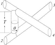
(c)

Figure 1: Three Feynman diagrams composed of two three-point vertices and a propagator called (a) $s$-channel, (b) $t$-channel, and (c) $u$-channel diagrams. The external legs should be read as semi-infinite cylinders. The line winding around the propagator denotes the contour along which $\xi$ and $b^{\pm}$ are integrated.

$$A^{stu}_{FFFF}= \kappa^{2}\int_{0}^{\infty}\!\!dT\!\!\int_{0}^{2\pi}\frac{d\theta}{2\pi}\Bigg{(}\langle(\eta\Psi_{1})(\eta\Psi_{2})\xi_{s}b_{s}^{+}b_{s}^{-}(\eta\Psi_{3})(\eta\Psi_{4})\rangle_{s}$$

$$+\langle(\eta\Psi_{1})(\eta\Psi_{3})\xi_{t}b_{t}^{+}b_{t}^{-}(\eta\Psi_{2})(\eta\Psi_{4})\rangle_{t}+\langle(\eta\Psi_{1})(\eta\Psi_{4})\xi_{u}b_{u}^{+}b_{u}^{-}(\eta\Psi_{2})(\eta\Psi_{3})\rangle_{u}\Bigg{)},$$ (94)

where the correlation function $\langle\cdots\rangle_{i=s,t,u}$ is evaluated as the conformal field theory (CFT) in the large Hilbert space on the $i$-channel Feynman diagram. The operators $\xi_{i}$ and $b^{\pm}_{i}$ inserted in each term are integrated along the contour winding around the propagator as depicted in Fig. 1. We can remove this $\xi$-insertion using an $\eta$ on an external state, for example $\eta\Psi_{1}$. As a result, the contribution (94) becomes

$$A^{stu}_{FFFF}= \kappa^{2}\int_{0}^{\infty}\!\!dT\!\!\int_{0}^{2\pi}\frac{d\theta}{2\pi}\Bigg{(}\langle\Psi_{1}(\eta\Psi_{2})b_{s}^{+}b_{s}^{-}(\eta\Psi_{3})(\eta\Psi_{4})\rangle_{s}$$

$$\hskip 28.45274pt+\langle\Psi_{1}(\eta\Psi_{3})b_{t}^{+}b_{t}^{-}(\eta\Psi_{2})(\eta\Psi_{4})\rangle_{t}+\langle\Psi_{1}(\eta\Psi_{4})b_{u}^{+}b_{u}^{-}(\eta\Psi_{2})(\eta\Psi_{3})\rangle_{u}\Bigg{)},$$

$$= \kappa^{2}\int_{F_{s}\cup F_{t}\cup F_{u}}d^{2}z_{1}\langle\xi U_{F}^{(-1/2)}(z_{1})V_{F}^{(-1/2)}(0)V_{F}^{(-1/2)}(1)V_{F}^{(-1/2)}(\infty)\rangle_{C},$$ (95)

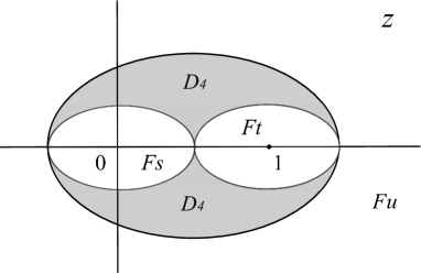
Figure 2: Complex plane

where, in the second equality, we conformally mapped the Feynman diagram to the complex plane[14, 15] depicted in Fig. 2. The external strings, one, two, three and four, are mapped to $z=z_{1}$, $0$, $1$, and $\infty$, respectively. The operator $V_{F}^{(-1/2)}$ is the conventional on-shell physical fermion vertex in the $-1/2$-picture[16] and related to the on-shell physical R state $|\Psi\rangle$ as $|\Psi\rangle=\xi_{0}V_{F}^{(-1/2)}(0)|0\rangle$. The integrated vertex operator $U_{F}$ is also the conventional one: $V_{F}=c\bar{c}U_{F}$. The correlation function $\langle\cdots\rangle_{C}$ of these operators is evaluated as the CFT on the complex plane, where the parameters $\{T,\theta\}$ of the Feynman diagram are mapped into the single complex moduli parameter $z_{1}$. The integration region coming from the $i$-channel $(i=s,t,u)$ contribution are depicted as $F_{i}$ in Fig. 2.

For $A_{FFFF}$, the last Feynman diagram depicted in Fig. 3 is drawn using the four-fermi interaction (92). The contribution from this diagram is

$$A_{FFFF}^{4}= \frac{\kappa^{2}}{4}\int d\theta_{a}d\theta_{b}\Bigg{(}\langle b_{C_{a}}b_{C_{b}}\Psi_{1}(\eta\Psi_{2})(\eta\Psi_{3})(\eta\Psi_{4})\rangle_{4}+\sum_{i=2}^{4}\langle\Psi(1)\rightarrow\Psi(i)\rangle_{4}\Bigg{)}$$

$$= \kappa^{2}\int_{D_{4}}d^{2}z_{1}\langle\xi U_{F}^{(-1/2)}(z_{1})V_{F}^{(-1/2)}(0)V_{F}^{(-1/2)}(1)V_{F}^{(-1/2)}(\infty)\rangle_{C},$$ (96)

where the correlation function in the first line is evaluated as the CFT on the diagram in Fig. 3. The moduli parameters $\{\theta_{a},\theta_{b}\}$ and corresponding anti-ghost insertions, $\{b_{C_{a}},b_{C_{b}}\}$, are the same as those given in Ref. Kugo:1989tk. In the second equality, we mapped the Feynman diagram to the complex plane and used the fact that the position of the $\xi(z)$ is irrelevant.[16] This contribution fills the shaded region $D_{4}$ in Fig. 2.

Figure 3: Feynman diagram using the four-point interaction

By summing up all of these contributions, the four-fermion amplitude $A_{FFFF}$ is finally given by integrating over the complete moduli space $\mathcal{M}_{(0,4)}=F_{s}\cup F_{t}\cup F_{u}\cup D_{4}$, the whole complex plane:

$$A_{FFFF}= A_{FFFF}^{stu}+A_{FFFF}^{4}$$

$$= \kappa^{2}\int_{\mathcal{M}_{(0,4)}}d^{2}z_{1}\langle\xi U_{F}^{(-1/2)}(z_{1})V_{F}^{(-1/2)}(0)V_{F}^{(-1/2)}(1)V_{F}^{(-1/2)}(\infty)\rangle_{C}.$$ (97)

This coincides with the well-known four-Ramond string amplitude.[16]

We can similarly show that the two-boson-two-fermion amplitude coincides with the well-known result. We suppose that the initial strings, strings one and two, are the NS strings and the final strings, strings three and four, are the R strings. In this case, the $s$-channel Feynman diagram consists of the three-boson vertex (89), the Yukawa vertex (90), and the NS propagator (84). Its contribution to the amplitudes is

$$A_{BBFF}^{s}= \frac{\kappa^{2}}{2}\int_{0}^{\infty}\!\!dT\!\!\int_{0}^{2\pi}\frac{d\theta}{2\pi}\Bigg{(}\langle(\eta V_{1})(QV_{2})\xi_{s}b_{s}^{+}b_{s}^{-}(\eta\Psi_{3})(\eta\Psi_{4})\rangle_{s}$$

$$\hskip 142.26378pt+\langle(QV_{1})(\eta V_{2})\xi_{s}b_{s}^{+}b_{s}^{-}(\eta\Psi_{3})(\eta\Psi_{4})\rangle_{s}\Bigg{)},$$

$$= \frac{\kappa^{2}}{2}\int_{0}^{\infty}\!\!dT\!\!\int_{0}^{2\pi}\frac{d\theta}{2\pi}\Bigg{(}\langle V_{1}(QV_{2})b_{s}^{+}b_{s}^{-}(\eta\Psi_{3})(\eta\Psi_{4})\rangle_{s}$$

$$\hskip 142.26378pt+\langle(QV_{1})V_{2}b_{s}^{+}b_{s}^{-}(\eta\Psi_{3})(\eta\Psi_{4})\rangle_{s}\Bigg{)},$$

$$= \frac{\kappa^{2}}{2}\int_{F_{s}}d^{2}z_{1}\Big{(}\langle\xi U_{B}^{(-1)}(z_{1})V_{B}^{(0)}(0)V_{F}^{-1/2}(1)V_{F}^{-1/2}(\infty)\rangle_{C}$$

$$\hskip 128.0374pt+\langle U_{B}^{(0)}(z_{1})\xi V_{B}^{(-1)}(0)V_{F}^{(-1/2)}(1)V_{F}^{(-1/2)}(\infty)\rangle_{C}\Big{)}.$$ (98)

Here, in a similar way to the four-fermion amplitudes, we eliminated $\xi$-insertion in the second equality by using the $\eta$ on the external NS state $\eta V_{1}$, and mapped the Feynman graph to the complex plane in the third equality. The boson vertex operator $V_{B}^{(-1)}$ is the conventional one in the $(-1)$-picture and related to the on-shell physical NS state $|V\rangle$ as $|V\rangle=\xi V_{B}(0)^{(-1)}|0\rangle$. The vertex $V_{B}^{(0)}$ in the $0$-picture also appears in (98) because $Q|V\rangle=V_{B}^{(0)}(0)|0\rangle$.[16] The integrated vertex $U_{B}$ is given by $V_{B}=c\bar{c}U_{B}$.

The other two, $t$-channel and $u$-channel, diagrams consist of the two Yukawa vertices (90) and the R propagator (85). Their contributions are

$$A_{BBFF}^{tu}= \frac{\kappa^{2}}{2}\int_{0}^{\infty}\!\!dT\!\!\int_{0}^{2\pi}\frac{d\theta}{2\pi}\Bigg{(}\langle(\eta V_{1})(\eta\Psi_{3})\xi_{t}b_{t}^{+}b_{t}^{-}(QV_{2})(\eta\Psi_{4})\rangle_{t}+\langle(QV_{1})(\eta\Psi_{3})\xi_{t}b_{t}^{+}b_{t}^{-}(\eta V_{2})(\eta\Psi_{4})\rangle_{t}$$

$$\hskip 56.9055pt+\langle(\eta V_{1})(\eta\Psi_{4})\xi_{u}b_{u}^{+}b_{u}^{-}(QV_{2})(\eta\Psi_{3})\rangle_{u}+\langle(QV_{1})(\eta\Psi_{4})\xi_{u}b_{u}^{+}b_{u}^{-}(\eta V_{2})(\eta\Psi_{3})\rangle_{u}\Bigg{)},$$

$$= \frac{\kappa^{2}}{2}\int_{0}^{\infty}\!\!dT\!\!\int_{0}^{2\pi}\frac{d\theta}{2\pi}\Bigg{(}\langle V_{1}(\eta\Psi_{3})b_{t}^{+}b_{t}^{-}(QV_{2})(\eta\Psi_{4})\rangle_{t}+\langle(QV_{1})(\eta\Psi_{3})b_{t}^{+}b_{t}^{-}V_{2}(\eta\Psi_{4})\rangle_{t}$$

$$\hskip 85.35826pt+\langle V_{1}(\eta\Psi_{4})b_{u}^{+}b_{u}^{-}(QV_{2})(\eta\Psi_{3})\rangle_{u}+\langle(QV_{1})(\eta\Psi_{4})b_{u}^{+}b_{u}^{-}V_{2}(\eta\Psi_{3})\rangle_{u}\Bigg{)},$$

$$= \frac{\kappa^{2}}{2}\int_{F_{t}\cup F_{u}}d^{2}z_{1}\Bigg{(}\langle\xi U_{B}^{(-1)}(z_{1})V_{B}^{(0)}(0)V_{F}^{(-1/2)}(1)V_{F}^{(-1/2)}(\infty)\rangle_{C}$$

$$\hskip 128.0374pt+\langle U_{B}^{(0)}(z_{1})\xi V_{B}^{(-1)}(0)V_{F}^{(-1/2)}(1)V_{F}^{(-1/2)}(\infty)\rangle_{C}\Bigg{)}.$$ (99)

The missing integration region $D_{4}$ is again filled by the contribution of the graph consisting of the four-string interaction (91),

$$A_{BBFF}^{4}= \frac{\kappa^{2}}{2}\int d\theta_{a}d\theta_{b}\Bigg{(}\langle b_{C_{a}}b_{C_{b}}V_{1}(z)(QV_{2})(\eta\Psi_{3})(\eta\Psi_{4})\rangle_{4}+\langle b_{C_{a}}b_{C_{b}}(QV_{1})V_{2}(\eta\Psi_{3})(\eta\Psi_{4})\rangle_{4}\Bigg{)},$$

$$= \frac{\kappa^{2}}{2}\int_{D_{4}}d^{2}z_{1}\Bigg{(}\langle\xi U_{B}^{(-1)}(z_{1})V_{B}^{(0)}(0)V_{F}^{(-1/2)}(1)V_{F}^{(-1/2)}(\infty)\rangle_{C}$$

$$\hskip 128.0374pt+\langle U_{B}^{(0)}(z_{1})\xi V_{B}^{(-1)}(0)V_{F}^{(-1/2)}(1)V_{F}^{(-1/2)}(\infty)\rangle_{C}\Bigg{)}.$$ (100)

As a result, the two-boson-two-fermion amplitude becomes the well-known form as

$$A_{BBFF}= A_{BBFF}^{s}+A_{BBFF}^{tu}+A_{BBFF}^{4}$$

$$= \frac{\kappa^{2}}{2}\int_{\mathcal{M}_{(0,4)}}d^{2}z_{1}\Bigg{(}\langle\xi U_{B}^{(-1)}(z_{1})V_{B}^{(0)}(0)V_{F}^{(-1/2)}(1)V_{F}^{(-1/2)}(\infty)\rangle_{C}$$

$$\hskip 85.35826pt+\langle U_{B}^{(0)}(z_{1})\xi V_{B}^{(-1)}(0)V_{F}^{(-1/2)}(1)V_{F}^{(-1/2)}(\infty)\rangle_{C}\Bigg{)},$$

$$= \kappa^{2}\int_{\mathcal{M}_{(0,4)}}d^{2}z_{1}\langle\xi U_{B}^{(-1)}(z_{1})V_{B}^{(0)}(0)V_{F}^{(-1/2)}(1)V_{F}^{(-1/2)}(\infty)\rangle_{C},$$ (101)

where in the last equality we used a $\xi$ manipulation,[16] which is only available if the moduli $z_{1}$ is integrated over the whole complex plane, $\mathcal{M}_{(0,4)}$.

6 Open questions and discussion

An important remaining problem is to prove the existence of a non-trivial solution to Eq. (55). If it has no non-trivial solution at some order in $\Psi$, we must relax the G-ansatz, for example by allowing the string field $\bar{B}_{\eta}(V)$ in (23) to appear in the correction terms. Then the general form (44) has to be modified.

A more important task is to give the complete equations of motion and the gauge transformations in a closed form. The general form (44) determined so as to be invariant under the $\Lambda_{0}$-gauge transformation (33) and consistent with the identity (28), or its alternative in the case mentioned above, will give an important clue in this study. In particular, the $\Omega$ seems to play an important role since it also appears in the constraint (77) and can be considered as a kind of non-linear extension of the R string field $\eta\Psi$ in the open superstring field theory.

It is also important to find the action giving the complete equations of motion. In this regard, it is worth noting that, in contrast to the equations of motion (i.e. $\Omega$ and $\Sigma$) (46), (54), and (59), not all the possible terms allowed by the ghost number and the picture number counting appear in the action (70) and (71). We conjecture, from the explicit form of $S_{R}^{(4)}$, (70), and $S_{R}^{(6)}$, (71), that each term in the R action includes the same number of $\Psi$s and $\Xi$s. Then, the possible terms in $S_{R}^{(2n+2)}$ take the form,

$$\kappa^{2n}\langle\eta\Psi,[\Psi,(Q_{G}\Psi)^{k_{1}},(Q_{G}\Xi)^{l_{1}},[\Psi,(Q_{G}\Psi)^{k_{2}},(Q_{G}\Xi)^{l_{2}},[\cdots,[\Psi,(Q_{G}\Psi)^{k_{m}},(Q_{G}\Xi)^{l_{m}}]_{G}\cdots]_{G}]_{G}]_{G}\rangle,$$

or that obtained by exchanging $\eta\Psi$ and one of the $Q_{G}\Xi$ in the middle ($2\geq i\geq m-1$) for $m\geq 3$, where $1\leq m\leq n$ and the non-negative integers $k_{i}$ and $l_{i}$ $(1\leq i\leq m)$ are restricted by $\sum_{i=1}^{m}k_{i}=n-m$, $\sum_{i=1}^{m}l_{i}=n+1$ and $k_{m}+l_{m}\neq 0$. Since these forms are much simpler than those of possible terms in the equations of motion, given in §4, it is interesting to look for some guiding principle to determine the action with the constraint without the help of the equations of motion.

Another remaining problem is to confirm that the Feynman rules constructed in §§5.1 reproduce general tree-level physical amplitudes since the proposed prescription has an ambiguity as already mentioned. The possible difficulty due to this ambiguity occurs when the $\omega$ in question is connected to the other vertex as an internal line, which first happens in the five-point amplitudes with the four external fermions. It must be confirmed whether this five-point amplitude is independent of the ambiguity or not. We might have to modify the Feynman rules, which seems to be suggested from the computation of the five-point amplitudes with external fermions in open superstring field theory.[17] Rules for computing loop amplitudes should also be found, which forces us to investigate the gauge-fixing procedure[18, 19] in more detail.

Appendix A The next-to-next-to-leading order corrections to the gauge transformations

In this Appendix, we give the explicit forms of the next-to-next-to-leading order corrections $\bar{B}_{\delta^{(6)}}$ and $\delta^{(4)}\Psi$ to the gauge transformations.

The next-to-next-to-leading order corrections to the $\Lambda_{1}$-gauge transformation are given by

$$\bar{B}_{\delta^{(6)}_{\Lambda_{1}}}(V)= -\frac{\kappa^{6}}{6!}[\Psi,(Q_{G}\Psi)^{2},(\eta\Psi)^{3},\eta\Lambda_{1}]_{G}-\frac{\kappa^{6}}{6!}[[\Psi,Q_{G}\Psi]_{G},\Psi,(\eta\Psi)^{3},\eta\Lambda_{1}]_{G}$$

$$-\frac{\kappa^{6}}{80}\kappa^{6}[[\Psi,\eta\Psi]_{G},\Psi,Q_{G}\Psi,(\eta\Psi)^{2},\eta\Lambda_{1}]_{G}-\frac{4}{6!}\kappa^{6}[[\Psi,Q_{G}\Psi,\eta\Psi]_{G},\Psi,(\eta\Psi)^{2},\eta\Lambda_{1}]_{G}$$

$$+\frac{4}{6!}\kappa^{6}[[\Psi,(\eta\Psi)^{2}]_{G},\Psi,Q_{G}\Psi,\eta\Psi,\eta\Lambda_{1}]_{G}-\frac{\kappa^{6}}{5!}[[\Psi,Q_{G}\Psi,(\eta\Psi)^{2}]_{G},\Psi,\eta\Psi,\eta\Lambda_{1}]_{G}$$

$$+\frac{\kappa^{6}}{6!}[[\Psi,(\eta\Psi)^{3}]_{G},\Psi,Q_{G}\Psi,\eta\Lambda_{1}]_{G}+\frac{2}{6!}\kappa^{6}[[\Psi,Q_{G}\Psi,(\eta\Psi)^{3}]_{G},\Psi,\eta\Lambda_{1}]_{G}$$

$$+\frac{2}{6!}\kappa^{6}[\Psi,[\Psi,Q_{G}\Psi,(\eta\Psi)^{3},\eta\Lambda_{1}]_{G}]_{G}+\frac{\kappa^{6}}{6!}[\Psi,Q_{G}\Psi,[\Psi,(\eta\Psi)^{3},\eta\Lambda_{1}]_{G}]_{G}$$

$$+\frac{\kappa^{6}}{80}[\Psi,\eta\Psi,[\Psi,Q_{G}\Psi,(\eta\Psi)^{2},\eta\Lambda_{1}]_{G}]_{G}+\frac{4}{6!}\kappa^{6}[\Psi,Q_{G}\Psi,\eta\Psi,[\Psi,(\eta\Psi)^{2},\eta\Lambda_{1}]_{G}]_{G}$$

$$+\frac{\kappa^{6}}{6!}[\Psi,(\eta\Psi)^{2},[\Psi,Q_{G}\Psi,\eta\Psi,\eta\Lambda_{1}]_{G}]_{G}+\frac{\kappa^{6}}{5!}[\Psi,Q_{G}\Psi,(\eta\Psi)^{2},[\Psi,\eta\Psi,\eta\Lambda_{1}]_{G}]_{G}$$

$$-\frac{\kappa^{6}}{6!}[\Psi,(\eta\Psi)^{3},[\Psi,Q_{G}\Psi,\eta\Lambda_{1}]_{G}]_{G}-\frac{5}{6!}\kappa^{6}[[\Psi,[\Psi,\eta\Psi]_{G}]_{G},\Psi,(\eta\Psi)^{2},\eta\Lambda_{1}]_{G}$$

$$+\frac{\kappa^{6}}{72}[[\Psi,[\Psi,(\eta\Psi)^{2}]_{G}]_{G},\Psi,\eta\Psi,\eta\Lambda_{1}]_{G}-\frac{\kappa^{6}}{48}[[\Psi,\eta\Psi,[\Psi,\eta\Psi]_{G}]_{G},\Psi,\eta\Psi,\eta\Lambda_{1}]_{G}$$

$$-\frac{\kappa^{6}}{48}[[\Psi,\eta\Psi]_{G},[\Psi,\eta\Psi]_{G},\Psi,\eta\Psi,\eta\Lambda_{1}]_{G}-\frac{\kappa^{6}}{6!}[[\Psi,[\Psi,(\eta\Psi)^{3}]_{G}]_{G},\Psi,\eta\Lambda_{1}]_{G}$$

$$-\frac{4}{6!}\kappa^{6}[[\Psi,\eta\Psi,[\Psi,(\eta\Psi)^{2}]_{G}]_{G},\Psi,\eta\Lambda_{1}]_{G}+\frac{\kappa^{6}}{80}[[\Psi,(\eta\Psi)^{2},[\Psi,\eta\Psi]_{G}]_{G},\Psi,\eta\Lambda_{1}]_{G}$$

$$+\frac{5}{6!}\kappa^{6}[[\Psi,\eta\Psi]_{G},[\Psi,(\eta\Psi)^{2}]_{G},\Psi,\eta\Lambda_{1}]_{G}+\frac{5}{6!}\kappa^{6}[\Psi,[\Psi,\eta\Psi]_{G},[\Psi,(\eta\Psi)^{2},\eta\Lambda_{1}]_{G}]_{G}$$

$$+\frac{\kappa^{6}}{80}[\Psi,[[\Psi,\eta\Psi]_{G},\Psi,(\eta\Psi)^{2},\eta\Lambda_{1}]_{G}]_{G}+\frac{\kappa^{6}}{48}[\Psi,\eta\Psi,[\Psi,\eta\Psi]_{G},[\Psi,\eta\Psi,\eta\Lambda_{1}]_{G}]_{G}$$

$$-\frac{4}{6!}\kappa^{6}[\Psi,[[\Psi,(\eta\Psi)^{2}]_{G},\Psi,\eta\Psi,\eta\Lambda_{1}]_{G}]_{G}+\frac{\kappa^{6}}{24}[\Psi,\eta\Psi,[[\Psi,\eta\Psi]_{G},\Psi,\eta\Psi,\eta\Lambda_{1}]_{G}]_{G}$$

$$-\frac{\kappa^{6}}{72}[\Psi,[\Psi,(\eta\Psi)^{2}]_{G},[\Psi,\eta\Psi,\eta\Lambda_{1}]_{G}]_{G}-\frac{\kappa^{6}}{6!}[\Psi,[[\Psi,(\eta\Psi)^{3}]_{G},\Psi,\eta\Lambda_{1}]_{G}]_{G}$$

$$-\frac{5}{6!}\kappa^{6}[\Psi,\eta\Psi,[[\Psi,(\eta\Psi)^{2}]_{G},\Psi,\eta\Lambda_{1}]_{G}]_{G}+\frac{5}{6!}\kappa^{6}[\Psi,(\eta\Psi)^{2},[[\Psi,\eta\Psi]_{G},\Psi,\eta\Lambda_{1}]_{G}]_{G}$$

$$-\frac{\kappa^{6}}{6!}[\Psi,[\Psi,[\Psi,(\eta\Psi)^{3},\eta\Lambda_{1}]_{G}]_{G}]_{G}-\frac{4}{6!}\kappa^{6}[\Psi,[\Psi,\eta\Psi,[\Psi,(\eta\Psi)^{2},\eta\Lambda_{1}]_{G}]_{G}]_{G}$$

$$-\frac{5}{6!}\kappa^{6}[\Psi,\eta\Psi,[\Psi,[\Psi,(\eta\Psi)^{2},\eta\Lambda_{1}]_{G}]_{G}]_{G}-\frac{\kappa^{6}}{5!}[\Psi,[\Psi,(\eta\Psi)^{2},[\Psi,\eta\Psi,\eta\Lambda_{1}]_{G}]_{G}]_{G}$$

$$-\frac{\kappa^{6}}{48}[\Psi,\eta\Psi,[\Psi,\eta\Psi,[\Psi,\eta\Psi,\eta\Lambda_{1}]_{G}]_{G}]_{G}a+\frac{5}{6!}\kappa^{6}[\Psi,(\eta\Psi)^{2},[\Psi,[\Psi,\eta\Psi,\eta\Lambda_{1}]_{G}]_{G}]_{G},$$ (102)

$$\delta^{(4)}_{\Lambda_{1}}\Psi= -\frac{\kappa^{5}}{5!}[\Psi,(Q_{G}\Psi)^{2},(\eta\Psi)^{2},\eta\Lambda_{1}]_{G}-\frac{\kappa^{5}}{5!}[[\Psi,Q_{G}\Psi]_{G},\Psi,(\eta\Psi)^{2},\eta\Lambda_{1}]_{G}$$

$$-\frac{7}{5!}\kappa^{5}[[\Psi,\eta\Psi]_{G},\Psi,Q_{G}\Psi,\eta\Psi,\eta\Lambda_{1}]_{G}-\frac{3}{5!}\kappa^{5}[[\Psi,Q_{G}\Psi,\eta\Psi]_{G},\Psi,\eta\Psi,\eta\Lambda_{1}]_{G}$$

$$+\frac{\kappa^{5}}{5!}[[\Psi,(\eta\Psi)^{2}]_{G},\Psi,Q_{G}\Psi,\eta\Lambda_{1}]_{G}-\frac{3}{5!}\kappa^{5}[[\Psi,Q_{G}\Psi,(\eta\Psi)^{2}]_{G},\Psi,\eta\Lambda_{1}]_{G}$$

$$+\frac{2}{5!}\kappa^{5}[\Psi,[\Psi,Q_{G}\Psi,(\eta\Psi)^{2},\eta\Lambda_{1}]_{G}]_{G}+\frac{\kappa^{5}}{5!}[\Psi,Q_{G}\Psi,[\Psi,(\eta\Psi)^{2},\eta\Lambda_{1}]_{G}]_{G}$$

$$+\frac{\kappa^{5}}{3\cdot 5!}[\Psi,\eta\Psi,[\Psi,Q_{G}\Psi,\eta\Psi,\eta\Lambda_{1}]_{G}]_{G}+\frac{3}{5!}\kappa^{5}[\Psi,Q_{G}\Psi,\eta\Psi,[\Psi,\eta\Psi,\eta\Lambda_{1}]_{G}]_{G}$$

$$-\frac{\kappa^{5}}{5!}[\Psi,(\eta\Psi)^{2},[\Psi,Q_{G}\Psi,\eta\Lambda_{1}]_{G}]_{G}-\frac{4}{5!}\kappa^{5}[[\Psi,[\Psi,\eta\Psi]_{G}]_{G},\Psi,\eta\Psi,\eta\Lambda_{1}]_{G}$$

$$+\frac{4}{5!}\kappa^{5}[[\Psi,[\Psi,(\eta\Psi)^{2}]_{G}]_{G},\Psi,\eta\Lambda_{1}]_{G}-\frac{\kappa^{5}}{15}[[\Psi,\eta\Psi,[\Psi,\eta\Psi]_{G}]_{G},\Psi,\eta\Lambda_{1}]_{G}$$

$$-\frac{\kappa^{5}}{15}[[\Psi,\eta\Psi]_{G},[\Psi,\eta\Psi]_{G},\Psi,\eta\Lambda_{1}]_{G}+\frac{7}{5!}\kappa^{5}[\Psi,[[\Psi,\eta\Psi]_{G},\Psi,\eta\Psi,\eta\Lambda_{1}]_{G}]_{G}$$

$$+\frac{4}{5!}\kappa^{5}[\Psi,[\Psi,\eta\Psi]_{G},[\Psi,\eta\Psi,\eta\Lambda_{1}]_{G}]_{G}-\frac{\kappa^{5}}{5!}[\Psi,[[\Psi,(\eta\Psi)^{2}]_{G},\Psi,\eta\Lambda_{1}]_{G}]_{G}$$

$$+\frac{\kappa^{5}}{45}[\Psi,\eta\Psi,[[\Psi,\eta\Psi]_{G},\Psi,\eta\Lambda_{1}]_{G}]_{G}-\frac{\kappa^{5}}{5!}[\Psi,[\Psi,[\Psi,(\eta\Psi)^{2},\eta\Lambda_{1}]_{G}]_{G}]_{G}$$

$$-\frac{3}{5!}\kappa^{5}[\Psi,[\Psi,\eta\Psi,[\Psi,\eta\Psi,\eta\Lambda_{1}]_{G}]_{G}]_{G}r+\frac{\kappa^{5}}{45}[\Psi,\eta\Psi,[\Psi,[\Psi,\eta\Psi,\eta\Lambda_{1}]_{G}]_{G}]_{G},$$ (103)

The same order corrections to the $\Lambda_{\frac{1}{2}}$-gauge transformations are obtained as

$$\bar{B}_{\delta^{(6)}_{\Lambda_{1/2}}}(V)= \frac{2}{3\cdot 5!}\kappa^{5}[\Psi,Q_{G}\Psi,(\eta\Psi)^{3},Q_{G}\Lambda_{\frac{1}{2}}]_{G}-\frac{\kappa^{5}}{5!}[[\Psi,Q_{G}\Psi,(\eta\Psi)^{3}]_{G},\Lambda_{\frac{1}{2}}]_{G}$$

$$+\frac{\kappa^{5}}{5!}[[\Psi,[\Psi,(\eta\Psi)^{3}]_{G}]_{G},\Lambda_{\frac{1}{2}}]_{G}+\frac{4}{5!}\kappa^{5}[[\Psi,\eta\Psi,[\Psi,(\eta\Psi)^{2}]_{G}]_{G},\Lambda_{\frac{1}{2}}]_{G}$$

$$-\frac{4}{5!}\kappa^{5}[[\Psi,(\eta\Psi)^{2},[\Psi,\eta\Psi]_{G}]_{G},\Lambda_{\frac{1}{2}}]_{G}+\frac{\kappa^{5}}{48}[[\Psi,\eta\Psi]_{G},\Psi,(\eta\Psi)^{2},Q_{G}\Lambda_{\frac{1}{2}}]_{G}$$

$$-\frac{\kappa^{5}}{36}[[\Psi,(\eta\Psi)^{2}]_{G},\Psi,\eta\Psi,Q_{G}\Lambda_{\frac{1}{2}}]_{G}-\frac{\kappa^{5}}{144}[[\Psi,(\eta\Psi)^{3}]_{G},\Psi,Q_{G}\Lambda_{\frac{1}{2}}]_{G}$$

$$-\frac{2}{3\cdot 5!}\kappa^{5}[\Psi,[\Psi,(\eta\Psi)^{3},Q_{G}\Lambda_{\frac{1}{2}}]_{G}]_{G}-\frac{\kappa^{5}}{48}[\Psi,\eta\Psi,[\Psi,(\eta\Psi)^{2},Q_{G}\Lambda_{\frac{1}{2}}]_{G}]_{G}$$

$$+\frac{\kappa^{5}}{72}[\Psi,(\eta\Psi)^{2},[\Psi,\eta\Psi,Q_{G}\Lambda_{\frac{1}{2}}]_{G}]_{G}+\frac{\kappa^{5}}{144}[\Psi,(\eta\Psi)^{3},[\Psi,Q_{G}\Lambda_{\frac{1}{2}}]_{G}]_{G},$$ (104)

$$\delta^{(4)}_{\Lambda_{1/2}}\Psi= \frac{\kappa^{4}}{40}[\Psi,Q_{G}\Psi,(\eta\Psi)^{2},Q_{G}\Lambda_{\frac{1}{2}}]_{G}$$

$$+\frac{\kappa^{4}}{15}[[\Psi,\eta\Psi]_{G},\Psi,\eta\Psi,Q_{G}\Lambda_{\frac{1}{2}}]_{G}-\frac{\kappa^{4}}{30}[[\Psi,(\eta\Psi)^{2}]_{G},\Psi,Q_{G}\Lambda_{\frac{1}{2}}]_{G}$$

$$-\frac{\kappa^{4}}{40}[\Psi,[\Psi,(\eta\Psi)^{2},Q_{G}\Lambda_{\frac{1}{2}}]_{G}]_{G}+\frac{2}{45}\kappa^{4}[\Psi,\eta\Psi,[\Psi,\eta\Psi,Q_{G}\Lambda_{\frac{1}{2}}]_{G}]_{G}$$

$$+\frac{\kappa^{4}}{30}[\Psi,(\eta\Psi)^{2},[\Psi,Q_{G}\Lambda_{\frac{1}{2}}]_{G}]_{G},$$ (105)

Those to the $\Lambda_{3/2}$-gauge transformations are

$$\bar{B}_{\delta^{(6)}_{\Lambda_{3/2}}}(V)= -\frac{2}{6!}\kappa^{5}[\Psi,Q_{G}\Psi,(\eta\Psi)^{3},\eta\Lambda_{\frac{3}{2}}]_{G}+\frac{2}{6!}\kappa^{5}[\Psi,[\Psi,(\eta\Psi)^{3},\eta\Lambda_{\frac{3}{2}}]_{G}]_{G}$$

$$+\frac{\kappa^{5}}{80}[\Psi,\eta\Psi,[\Psi,(\eta\Psi)^{2},\eta\Lambda_{\frac{3}{2}}]_{G}]_{G}+\frac{\kappa^{5}}{6!}[\Psi,(\eta\Psi)^{2},[\Psi,\eta\Psi,\eta\Lambda_{\frac{3}{2}}]_{G}]_{G}$$

$$-\frac{\kappa^{5}}{6!}[\Psi,(\eta\Psi)^{3},[\Psi,\eta\Lambda_{\frac{3}{2}}]_{G}]_{G}-\frac{\kappa^{5}}{80}[[\Psi,\eta\Psi]_{G},\Psi,(\eta\Psi)^{2},\eta\Lambda_{\frac{3}{2}}]_{G}$$

$$+\frac{4}{6!}\kappa^{5}[[\Psi,(\eta\Psi)^{2}]_{G},\Psi,\eta\Psi,\eta\Lambda_{\frac{3}{2}}]_{G}+\frac{\kappa^{5}}{6!}[[\Psi,(\eta\Psi)^{3}]_{G},\Psi,\eta\Lambda_{\frac{3}{2}}]_{G},$$ (106)

$$\delta^{(4)}_{\Lambda_{3/2}}\Psi= -\frac{2}{5!}\kappa^{4}[\Psi,Q_{G}\Psi,(\eta\Psi)^{2},\eta\Lambda_{\frac{3}{2}}]_{G}+\frac{2}{5!}\kappa^{4}[\Psi,[\Psi,(\eta\Psi)^{2},\eta\Lambda_{\frac{3}{2}}]_{G}]_{G}$$

$$+\frac{\kappa^{4}}{3\cdot 5!}[\Psi,\eta\Psi,[\Psi,\eta\Psi,\eta\Lambda_{\frac{3}{2}}]_{G}]_{G}-\frac{\kappa^{4}}{5!}[\Psi,(\eta\Psi)^{2},[\Psi,\eta\Lambda_{\frac{3}{2}}]_{G}]_{G}$$

$$-\frac{7}{5!}\kappa^{4}[[\Psi,\eta\Psi]_{G},\Psi,\eta\Psi,\eta\Lambda_{\frac{3}{2}}]_{G}+\frac{\kappa^{4}}{5!}[[\Psi,(\eta\Psi)^{2}]_{G},\Psi,\eta\Lambda_{\frac{3}{2}}]_{G}.$$ (107)

Appendix B Derivation of Eq. (44)

Let us start to consider the correction to the equations of motion

$$\eta G =0,$$ (108)

$$Q_{G}\eta\Psi =0.$$ (109)

Since the left-hand sides of these equations are identically annihilated by $Q_{G}$, the correction terms have to be also annihilated by $Q_{G}$ at least up to the equations of motion. We can classify the correction terms into two categories depending on whether they are annihilated by $Q_{G}$ without using the equations of motion or not. Since the terms, composed of general off-shell string fields, identically annihilated by $Q_{G}$ have to be $Q_{G}$-exact, let us write them $Q_{G}\Sigma$ and $Q_{G}(\Omega-\eta\Psi)$ for the NS and the R equations of motion, respectively. Then the full equations of motion become the form

$$\eta G+Q_{G}\Sigma+E_{NS} =0,$$ (110a)

$$Q_{G}\Omega+E_{R} =0,$$ (110b)

where $E_{NS}$ and $E_{R}$ are the correction terms in the second category, which have to be self-consistently determined in such a way that $Q_{G}E_{NS}$ and $Q_{G}E_{R}$ are proportional to (the left-hand side of) these equations of motion (110) themselves.

Now let us first determine $E_{R}$. Under the G-ansatz, we can suppose, without loss of generality, that the possible terms in $E_{R}$ take the form of those obtained by replacing one of the $\Psi$s in the general possible terms in $\Omega$, given in §3, with $Q_{G}\Psi$. One can deduce that $Q_{G}E_{R}$ must be proportional to the R equation of motion (110b) from the form of these general terms. Then, from the (non-) linearity of $Q_{G}$ acting on the two (more than two) string products, the possible form of $E_{R}$ has to be

$$E_{R}=[\Omega,Q_{G}A]_{G}+[[\Omega,A]_{G},Q_{G}A]_{G}+\cdots,$$ (111)

where $A$ is a string field with Grassmann odd and the ghost and picture numbers $(G,P)=(1,0)$. The terms represented by dots can be iteratively determined so that $Q_{G}E_{R}$ is proportional to the R equation of motion (110b). We cannot, however, construct such a string field $A$ with the desired ghost and picture numbers, and hence $E_{R}\equiv 0$. We can similarly determine the $E_{NS}$, using the fact that $E_{R}\equiv 0$, as

$$E_{NS}=-\frac{\kappa}{2}[\Omega^{2}]_{G},$$ (112)

where the numerical coefficient is fixed to reproduce the leading correction term (30).

In conclusion, consistency with the identity (28) requires the full equations of motion to be in the form of (44) under the G-ansatz.

Appendix C Derivation of Eq. (60) and the explicit forms of $\bar{B}^{[2]}_{\delta}$

From the forms of the fundamental possible terms (47), the terms built with the one string product in the $\Omega^{(2n+1)}$ and the $\Sigma^{(2n+2)}$ and the terms with two string products in the $\Sigma^{(2n+2)}$ can be written for $n\geq 1$ as

$$\Omega^{(2n+1)}= \kappa^{2n}f_{n}[\Psi,(Q_{G}\Psi)^{n-1},(\eta\Psi)^{n+1}]_{G}+\cdots,$$ (113)

$$\Sigma^{(2n+2)}= \kappa^{2n+1}g_{n}[\Psi,(Q_{G}\Psi)^{n-1},(\eta\Psi)^{n+2}]_{G}$$

$$+\kappa^{2n+1}\underset{(m,l)\neq(0,0)}{\sum_{m=0}^{n-2}\sum_{l=0}^{n+2}}g_{n,m,l}[\Psi,(Q_{G}\Psi)^{n-m-2},(\eta\Psi)^{n-l+2},[\Psi,(Q_{G}\Psi)^{m},(\eta\Psi)^{l}]_{G}]_{G}+\cdots,$$ (114)

where $f_{n}$, $g_{n}$ and $g_{n,m,l}$ are the numerical coefficients to be determined and the dots represent the terms with greater numbers of string products. The terms built with the two string products in the $\Sigma^{(2n+2)}$ only exist for $n\geq 2$. The consistency equation (55) requires, neglecting the terms with more than two string products, that the following equations hold:

$$f_{1}=-4g_{1},\qquad g_{1}=\frac{1}{4!},$$

$$\left(\begin{array}[]{c}n-1\\ m\end{array}\right)\left(\begin{array}[]{c}n+3\\ l\end{array}\right)g_{n}+g_{n,m,l-1}-g_{n,m-1,l}$$ (119)

$$\hskip 142.26378pt+2(n-m+1)g_{n-m}f_{m}\delta_{l,m+1}-g_{n-m-1}g_{m}\delta_{l,m+2}=0,$$

$$\hskip 213.39566pt(n\geq 2,\ 0\leq m\leq n-2,\ 1\leq l\leq n+2),$$

$$\left(\begin{array}[]{c}n+3\\ l\end{array}\right)g_{n}-g_{n,n-2,l}+\frac{1}{3!}f_{n-1}\delta_{l,n}-\frac{1}{2}g_{n-1}\delta_{l,n+1}+f_{n}\delta_{l,n+2}=0,$$ (122)

$$\hskip 284.52756pt(n\geq 3,\ 1\leq l\leq n+2),$$

$$\left(\begin{array}[]{c}n-1\\ m+1\end{array}\right)g_{n}-g_{n,m,0}=0,\hskip 85.35826pt(n\geq 3,\ 1\leq m\leq n-2),$$ (125)

$$\left(\begin{array}[]{c}n-1\\ m\end{array}\right)g_{n}+g_{n,m,n+2}=0,\hskip 56.9055pt(n\geq 3,\ 1\leq m\leq n-2).$$ (128)

All the coefficients $f_{n}$, $g_{n}$ and $g_{n,m,l}$ are uniquely determined by solving these equations as

$$f_{n}=-\frac{1}{(2n+1)!},\qquad g_{n}=\frac{1}{(2n+2)!},$$

$$g_{n,m,l}=\begin{cases}\displaystyle\sum_{k=0}^{l}\left(\begin{array}[]{c}n-1\\ m+l+1-k\end{array}\right)\left(\begin{array}[]{c}n+3\\ k\end{array}\right)\frac{1}{(2n+2)!},&\textrm{for}\ 0\leq l\leq m+1,\\ \displaystyle-\sum_{k=0}^{m}\left(\begin{array}[]{c}n-1\\ k\end{array}\right)\left(\begin{array}[]{c}n+3\\ m+l+1-k\end{array}\right)\frac{1}{(2n+2)!},&\textrm{for}\ m+2\leq l\leq n+2,\end{cases}$$ (129)

with the help of the formula:

$$\sum_{r=0}^{p}\left(\begin{array}[]{c}n\\ r\end{array}\right)\left(\begin{array}[]{c}m\\ p-r\end{array}\right)=\left(\begin{array}[]{c}n+m\\ p\end{array}\right)\ \textrm{for}\ p\leq n+m.$$ (130)

The explicit forms of the terms with two string products, $\bar{B}^{[2]}_{\delta}(V)$, in the gauge transformations of $V$ are given by

$$\bar{B}^{[2]}_{\delta_{\Lambda_{1}}}(V)= -\sum_{n=3}^{\infty}\sum_{m=1}^{n-2}\sum_{l=0}^{n+1}\left(g_{n,m,l}+\left(\begin{array}[]{c}n-1\\ m\end{array}\right)\left(\begin{array}[]{c}n+2\\ l\end{array}\right)g_{n}\right)$$ (135)

$$\hskip 42.67912pt\times\kappa^{2n+2}[\Psi,(Q_{G}\Psi)^{n-m-1},(\eta\Psi)^{n-l+1},[\Psi,(Q_{G}\Psi)^{m},(\eta\Psi)^{l},\eta\Lambda_{1}]_{G}]_{G}$$

$$+\sum_{n=2}^{\infty}\sum_{l=1}^{n+1}\left(\begin{array}[]{c}n+2\\ l+1\end{array}\right)g_{n}\kappa^{2n+2}[\Psi,(Q_{G}\Psi)^{n-1},(\eta\Psi)^{n-l+1},[\Psi,(\eta\Psi)^{l},\eta\Lambda_{1}]_{G}]_{G}$$ (138)

$$-\sum_{n=3}^{\infty}\sum_{l=0}^{n+1}\left(\begin{array}[]{c}n+2\\ l\end{array}\right)g_{n}\kappa^{2n+2}[\Psi,(\eta\Psi)^{n-l+1},[\Psi,(Q_{G}\Psi)^{n-1},(\eta\Psi)^{l},\eta\Lambda_{1}]_{G}]_{G}$$ (141)

$$+\sum_{n=3}^{\infty}\sum_{m=1}^{n-2}g_{n-m-1}g_{m}$$

$$\hskip 42.67912pt\times\kappa^{2n+2}[\Psi,(Q_{G}\Psi)^{n-m-1},(\eta\Psi)^{n-m},[\Psi,(Q_{G}\Psi)^{m},(\eta\Psi)^{m+1},\eta\Lambda_{1}]_{G}]_{G}$$

$$-\sum_{n=3}^{\infty}\sum_{m=1}^{n-2}(n-m)g_{n-m}f_{m}$$

$$\hskip 42.67912pt\times\kappa^{2n+2}[\Psi,(Q_{G}\Psi)^{n-m-1},(\eta\Psi)^{n-m+1},[\Psi,(Q_{G}\Psi)^{m},(\eta\Psi)^{m},\eta\Lambda_{1}]_{G}]_{G}$$

$$-\sum_{n=1}^{\infty}f_{n}\kappa^{2n+2}[\Psi,[\Psi,(Q_{G}\Psi)^{n-1},(\eta\Psi)^{n+1},\eta\Lambda_{1}]_{G}]_{G}$$

$$+\sum_{n=1}^{\infty}\frac{1}{2}g_{n-1}\kappa^{2n+2}[\Psi,\eta\Psi,[\Psi,(Q_{G}\Psi)^{n-1},(\eta\Psi)^{n},\eta\Lambda_{1}]_{G}]_{G}$$

$$-\sum_{n=3}^{\infty}\frac{1}{4!}f_{n-1}\kappa^{2n+2}[\Psi,(\eta\Psi)^{2},[\Psi,(Q_{G}\Psi)^{n-1},(\eta\Psi)^{n-1},\eta\Lambda_{1}]_{G}]_{G}$$

$$-\frac{3}{4!}\kappa^{4}[\Psi,[\Psi,(\eta\Psi)^{2},\eta\Lambda_{1}]_{G}]_{G}-\frac{3}{4!}\kappa^{4}[\Psi,\eta\Psi,[\Psi,\eta\Psi,\eta\Lambda_{1}]_{G}]_{G}$$

$$-\frac{4}{6!}\kappa^{6}[\Psi,[\Psi,Q_{G}\Psi,(\eta\Psi)^{3},\eta\Lambda_{1}]_{G}]_{G}-\frac{\kappa^{6}}{5!}[\Psi,\eta\Psi,[\Psi,Q_{G}\Psi,(\eta\Psi)^{2},\eta\Lambda_{1}]_{G}]_{G}$$

$$+\frac{\kappa^{6}}{6!}[\Psi,(\eta\Psi)^{2},[\Psi,Q_{G}\Psi,\eta\Psi,\eta\Lambda_{1}]_{G}]_{G}-\frac{\kappa^{6}}{6!}[\Psi,(\eta\Psi)^{3},[\Psi,Q_{G}\Psi,\eta\Lambda_{1}]_{G}]_{G}$$

$$-\sum_{n=3}^{\infty}\sum_{m=1}^{n-2}\sum_{l=0}^{n+1}\left(g_{n,m,l}+\left(\begin{array}[]{c}n-1\\ m\end{array}\right)\left(\begin{array}[]{c}n+2\\ l\end{array}\right)g_{n}\right)$$ (146)

$$\hskip 42.67912pt\times\kappa^{2n+2}[[\Psi,(Q_{G}\Psi)^{m},(\eta\Psi)^{l}]_{G},\Psi,(Q_{G}\Psi)^{n-m-1},(\eta\Psi)^{n-l+2},\eta\Lambda_{1}]_{G}$$

$$+\sum_{n=2}^{\infty}\sum_{l=1}^{n+1}\left(\begin{array}[]{c}n+2\\ l+1\end{array}\right)g_{n}\kappa^{2n+2}[[\Psi,(\eta\Psi)^{l}]_{G},\Psi,(Q_{G}\Psi)^{n-1},(\eta\Psi)^{n-l+1},\eta\Lambda_{1}]_{G}$$ (149)

$$-\sum_{n=3}^{\infty}\sum_{l=0}^{n+1}g_{n}\kappa^{2n+2}[[\Psi,(Q_{G}\Psi)^{n-1},(\eta\Psi)^{l}]_{G},\Psi(\eta\Psi)^{n-l+1},\eta\Lambda_{1}]_{G}$$

$$-\sum_{n=2}^{\infty}\frac{1}{2}g_{n-1}\kappa^{2n+2}[[\Psi,\eta\Psi]_{G},\Psi,(Q_{G}\Psi)^{n-1},(\eta\Psi)^{n},\eta\Lambda_{1}]_{G}$$

$$-\frac{3}{4!}\kappa^{4}[[\Psi,\eta\Psi]_{G},\Psi,\eta\Psi,\eta\Lambda_{1}]_{G}+\frac{\kappa^{4}}{4!}[[\Psi,(\eta\Psi)^{2}]_{G},\Psi,\eta\Lambda_{1}]_{G}$$

$$-\frac{\kappa^{6}}{6!}[[\Psi,Q_{G}\Psi]_{G},\Psi,(\eta\Psi)^{3},\eta\Lambda_{1}]_{G}-\frac{4}{6!}\kappa^{6}[[\Psi,Q_{G}\Psi,\eta\Psi]_{G},\Psi,(\eta\Psi)^{2},\eta\Lambda_{1}]_{G}$$

$$-\frac{\kappa^{6}}{5!}[[\Psi,Q_{G}\Psi,(\eta\Psi)^{2}]_{G},\Psi,\eta\Psi,\eta\Lambda_{1}]_{G}+\frac{2}{6!}\kappa^{6}[[\Psi,Q_{G}\Psi,(\eta\Psi)^{3}]_{G},\Psi,\eta\Lambda_{1}]_{G},$$ (150)

for the $\Lambda_{1}$-gauge transformation,

$$\bar{B}^{[2]}_{\delta_{\Lambda_{1/2}}}(V)= \sum_{n=1}^{\infty}f_{n}\kappa^{2n+1}[[\Psi,(Q_{G}\Psi)^{n-1},(\eta\Psi)^{n+1}]_{G},\Lambda_{\frac{1}{2}}]_{G}$$

$$+\sum_{n=2}^{\infty}\sum_{m=0}^{n-2}\sum_{l=0}^{n+1}(n-l+2)g_{n,m,l}$$

$$\hskip 42.67912pt\times\kappa^{2n+1}[[\Psi,(Q_{G}\Psi)^{m},(\eta\Psi)^{l}]_{G},\Psi,(Q_{G}\Psi)^{n-m-2},(\eta\Psi)^{n-l+1},Q_{G}\Lambda_{\frac{1}{2}}]_{G}$$

$$+\sum_{n=2}^{\infty}\sum_{m=0}^{n-2}\sum_{l=0}^{n+2}lg_{n,m,l}$$

$$\hskip 42.67912pt\times\kappa^{2n+1}[\Psi,(Q_{G}\Psi)^{n-m+2},(\eta\Psi)^{n-l+2},[\Psi,(Q_{G}\Psi)^{m},(\eta\Psi)^{l-1},Q_{G}\Lambda_{\frac{1}{2}}]_{G}]_{G}$$

$$-\sum_{n=2}^{\infty}\sum_{m=0}^{n-2}(n-m+1)(m+2)g_{n-m-1}f_{m+1}$$

$$\hskip 42.67912pt\times\kappa^{2n+1}[\Psi,(Q_{G}\Psi)^{n-m+2},(\eta\Psi)^{n-m},[\Psi,(Q_{G}\Psi)^{m},(\eta\Psi)^{m+1},Q_{G}\Lambda_{\frac{1}{2}}]_{G}]_{G},$$ (151)

for the $\Lambda_{1/2}$-gauge transformation, and

$$\bar{B}_{\delta_{\Lambda_{3/2}}}^{[2]}(V)= -\sum_{n=3}^{\infty}\sum_{m=1}^{n-2}\sum_{l=0}^{n+1}\left((n-m-1)g_{n,m,l}+(n-1)\left(\begin{array}[]{c}n-2\\ m\end{array}\right)\left(\begin{array}[]{c}n+2\\ l\end{array}\right)g_{n}\right)$$ (156)

$$\hskip 42.67912pt\times\kappa^{2n+1}[[\Psi,(Q_{G}\Psi)^{m},(\eta\Psi)^{l}]_{G},\Psi,(Q_{G}\Psi)^{n-m-2},(\eta\Psi)^{n-l+2},\eta\Lambda_{\frac{3}{2}}]_{G}$$

$$+\sum_{n=2}^{\infty}\sum_{l=1}^{n+1}(n-1)\left(\begin{array}[]{c}n+2\\ l+1\end{array}\right)g_{n}$$ (159)

$$\hskip 42.67912pt\times\kappa^{2n+1}[[\Psi,(\eta\Psi)^{l}]_{G},\Psi,(Q_{G}\Psi)^{n-2},(\eta\Psi)^{n-l+1},\eta\Lambda_{\frac{3}{2}}]_{G}$$

$$-\sum_{n=2}^{\infty}\frac{1}{2}(n-1)g_{n-1}\kappa^{2n+1}[[\Psi,\eta\Psi]_{G},\Psi,(Q_{G}\Psi)^{n-2},(\eta\Psi)^{n},\eta\Lambda_{\frac{3}{2}}]_{G}$$

$$-\sum_{n=3}^{\infty}\sum_{m=0}^{n-3}\sum_{l=1}^{n+2}\left((m+1)g_{n,m,l}-(n-1)\left(\begin{array}[]{c}n-2\\ m\end{array}\right)\left(\begin{array}[]{c}n+2\\ l\end{array}\right)g_{n}\right)$$ (164)

$$\hskip 42.67912pt\times\kappa^{2n+1}[\Psi,(Q_{G}\Psi)^{n-m-2},(\eta\Psi)^{n-l+2},[\Psi,(Q_{G}\Psi)^{m},(\eta\Psi)^{l-1},\eta\Lambda_{\frac{3}{2}}]_{G}]_{G}$$

$$+\sum_{n=3}^{\infty}\sum_{m=0}^{n-3}(n-m+1)(m+1)g_{n-m-1}f_{m+1}$$

$$\hskip 42.67912pt\times\kappa^{2n+1}[\Psi,(Q_{G}\Psi)^{n-m-2},(\eta\Psi)^{n-m},[\Psi,(Q_{G}\Psi)^{m},(\eta\Psi)^{m+1},\eta\Lambda_{\frac{3}{2}}]_{G}]_{G}$$

$$-\sum_{n=2}^{\infty}\sum_{l=1}^{n+2}(n-1)\left(\begin{array}[]{c}n+2\\ l-1\end{array}\right)g_{n}$$ (167)

$$\hskip 42.67912pt\times\kappa^{2n+1}[\Psi,(\eta\Psi)^{n-l+2},[\Psi,(Q_{G}\Psi)^{n-2},(\eta\Psi)^{l-1},\eta\Lambda_{\frac{3}{2}}]_{G}]_{G}$$

$$-\sum_{n=2}^{\infty}(n-1)f_{n}\kappa^{2n+1}[\Psi,[\Psi,(Q_{G}\Psi)^{n-2},(\eta\Psi)^{n+1},\eta\Lambda_{\frac{3}{2}}]_{G}]_{G}$$

$$+\sum_{n=2}^{\infty}\frac{1}{2}(n-1)g_{n-1}\kappa^{2n+1}[\Psi,\eta\Psi,[\Psi,(Q_{G}\Psi)^{n-2},(\eta\Psi)^{n},\eta\Lambda_{\frac{3}{2}}]_{G}]_{G}$$

$$-\sum_{n=2}^{\infty}\frac{1}{4!}(n-1)f_{n-1}\kappa^{2n+1}[\Psi,(\eta\Psi)^{2},[\Psi,(Q_{G}\Psi)^{n-2},(\eta\Psi)^{n-1},\eta\Lambda_{\frac{3}{2}}]_{G}]_{G},$$ (168)

for the $\Lambda_{3/2}$-gauge transformation.

References

- [1] Y. Okawa and B. Zwiebach, J. High Energy Phys. 0407, 042 (2004) [hep-th/0406212].
- [2] N. Berkovits, Y. Okawa, and B. Zwiebach, J. High Energy Phys. 0411, 038 (2004) [hep-th/0409018].
- [3] N. Berkovits, Nucl. Phys. B 450, 90 (1995)[hep-th/9503099]; Nucl. Phys. B 459, 439 (1996)[erratum].
- [4] M. Saadi and B. Zwiebach, Annals Phys. 192, 213 (1989).
- [5] M. Kaku, Phys. Rev. D38 3052 (1988).
- [6] M. Kaku and J. Lykken, Phys. Rev. D38, 3067 (1988).
- [7] T. Kugo, H. Kunitomo, and K. Suehiro, Phys. Lett. B226, 48 (1989).
- [8] T. Kugo and K. Suehiro, Nucl. Phys. B 337, 434 (1990).
- [9] B. Zwiebach, Nucl. Phys. B 390, 33 (1993) [hep-th/9206084].
- [10] N. Berkovits, J. High Energy Phys. 0111, 047 (2001) [hep-th/0109100].
- [11] Y. Michishita, J. High Energy Phys. 0501, 012 (2005) [hep-th/0412215].
- [12] N. Berkovits and C. Vafa, Nucl. Phys. B 433 (1995) 123 [hep-th/9407190].
- [13] H. Hata, K. Itoh, T. Kugo, H. Kunitomo, and K. Ogawa, Prog. Theor. Phys. 78, 453 (1987).
- [14] A. LeClair, M. E. Peskin and C. R. Preitschopf, Nucl. Phys. B 317, 411 (1989).
- [15] A. LeClair, M. E. Peskin and C. R. Preitschopf, Nucl. Phys. B 317, 464 (1989).
- [16] D. Friedan, E. J. Martinec and S. H. Shenker, Nucl. Phys. B 271, 93 (1986).
-
[17]
Y. Michishita, Talk given at “String Field Theory 07”, RIKEN,
6-7 October 2007.
(Available at http://www.riken.jp/lab-www/theory/sft/sft07_michishita.pdf, date last accessed February 19, 2014.) - [18] M. Kroyter, Y. Okawa, M. Schnabl, S. Torii, and B. Zwiebach, JHEP 1203, 030 (2012) [arXiv:1201.1761 [hep-th]].
- [19] N. Berkovits, JHEP 1203, 012 (2012) [arXiv:1201.1769 [hep-th]].