Inference on Dynamic Models for non-Gaussian Random Fields using INLA: A Homicide Rate Anaysis of Brazilian Cities

Abstract

Robust time series analysis is an important subject in statistical modeling. Models based on Gaussian distribution are sensitive to outliers, which may imply in a significant degradation in estimation performance as well as in prediction accuracy. State-space models, also referred as Dynamic Models, is a very useful way to describe the evolution of a time series variable through a structured latent evolution system. Integrated Nested Laplace Approximation (INLA) is a recent approach proposed to perform fast approximate Bayesian inference in Latent Gaussian Models which naturally comprises Dynamic Models. We present how to perform fast and accurate non-Gaussian dynamic modeling with INLA and show how these models can provide a more robust time series analysis when compared with standard dynamic models based on Gaussian distributions. We formalize the framework used to fit complex non-Gaussian space-state models using the R package INLA and illustrate our approach in both a simulation study and a Brazilian homicide rate dataset.

arXiv:0000.0000

, , and

a]Department of Statistics, Universidade Federal de Minas Gerais b]Department of Mathematical Sciences, Norwegian University of Science and Technology c]Department of Sociology, Universidade Federal de Minas Gerais

1 Introduction

Robust estimation of time series analysis is an important and challenging field of statistical application from either frequentist (bustos1986; denby1979) or Bayesian perspectives (west1981). Such models are preferred when the dataset under study is affected by structural or abrupt changes. Dynamic Linear Models (DLM) and Generalized Dynamic Linear Models (DGLM), also referred as state-space models, are a broad class of parametric models that generalizes regression and time series models with time varying parameters, where both the parameter variation and the observed data are described in an evolution structured way (migon2005). Dynamic models are composed by an observational equation and one or more system equations in which the error terms are usually chosen to follow a Gaussian distribution. However, it is well known that the Gaussian distribution is very sensitive to outliers, which may produce degradation in the estimation performance (fox1972). Therefore, one might be interested in building a more flexible model based on heavy-tailed distributions rather than the usual Gaussian. Such models fall into the class of non-Gaussian dynamic models (see, kitagawa1987non; durbin2000 for a detailed description as well as applications of this class of models).

Integrated Nested Laplace Approximation (INLA) is an approach proposed by rue2009approximate to perform approximate fully Bayesian inference in the class of latent Gaussian models (LGMs). LGMs is a broad class and include many of the standard models currently in use by the applied community, e.g., stochastic volatility, disease mapping, log-Gaussian Cox process and generalized linear models. As opposed to the simulation-based methods, like Markov Chain Monte Carlo (MCMC), INLA performs approximate inference using a series of deterministic approximations that take advantage of the LGM structure to provide fast and accurate approximations. Moreover, it avoids known problems with commonly used simulation-based methods, e.g., difficulty in diagnosing convergence, additive Monte Carlo errors, and high demand in terms of computational time. Even for dynamic models within the class of LGMs, it was not possible to fit most of them using the available tools in the INLA package for R, hereafter denoted as R-INLA. ruiz2011direct presented a general framework which enabled users to use R-INLA to perform fully Bayesian inference for a variety of state-space models. However, their approach does not include the class of non-Gaussian dynamic models where the errors of the system equations have a non-Gaussian distribution as, for example, the heavy-tailed distributions.

One of the key assumptions of the INLA approach is that the latent field follows a Gaussian distribution. However, martins2014extendingScan have shown a way to extend INLA to cases where some independent components of the latent field have a non-Gaussian distribution. Their approach transfer the non-Gaussianity of the latent field to the likelihood function and it has shown to produce satisfactory results as long as this distribution is not far from Gaussian. Distributions that add flexibility around a Gaussian as near-Gaussian distributions are referred as being, for example, unimodal and symmetric.

The contribution of this paper is three folded: 1) Extend INLA for non-Gaussian latent models with dependent structure, specifically for non-Gaussian DLMs; 2) Present in a simple manner how to use R-INLA to perform non-Gaussian DLMs modelling. To accomplish these issues, we introduce a reparametrization of the non-Gaussian DLM and combine with the computational framework provided by R-INLA to introduce how to model dependent non-Gaussian latent field in the R-INLA setup; 3) We analyze the Brazilian homicides rates using a robust approach. The analysis indicates that, in most of our application scenarios, the robust method outperforms the traditional Gaussian approach.

The paper is organized as following: Section 2 introduces the methodology of our approach, presenting how to perform fast Bayesian inference using R-INLA for non-Gaussian DLMs. Section 3 presents our simulation study to compare two competitor models using some quality measures. In Section 4 we present the study over the Brazilian Homicide data, explaining our findings. Finally, in Section 5 we discuss some final remarks and future research.

2 Methodology

This Section will describe our approach to handle non-Gaussian DLM within R-INLA. Although valid for DGLM, we have chosen to illustrate our extension using a DLM to facilitate the presentation. To apply the extension for DGLM, a simple change in the Gaussian likelihood is necessary, which is a trivial modification under R-INLA. Section 2.1 will define a general DLM of interest, and show that it fits the class of LGM only if the error terms of the system equations are Gaussian distributed. Section 2.2 will review the INLA methodology, including the recent extension that allows INLA to be applied to models where some components of the latent field have non-Gaussian distribution. Section 2.3 gives an overview of a generic approach to fit dynamic models using R-INLA through an augmented model structure. Finally, Section 2.4 extend the approaches presented in Sections 2.2 and 2.3 and show how this extension can be exploited to fit non-Gaussian DLM within R-INLA.

2.1 Models

INLA approach performs approximate Bayesian inference in latent Gaussian models where the first stage is formed by the likelihood function with conditional independence properties given the latent field $\boldsymbol{x}$ and possible hyperparameters $\boldsymbol{\theta}_{1}$, where each data point $\{y_{t},\ t=1,...,n_{d}\}$ is connected to one element in the latent field. In this context, the latent field $\boldsymbol{x}$ is formed by linear predictors, random and fixed effects, depending on the model formulation. Assuming that the elements of the latent field connected to the data points, i.e., the linear predictors $\{\eta_{t},\ t=1,...,n_{d}\}$, are positioned on the first $n_{d}$ elements of $\boldsymbol{x}$, we have

• Stage 1. $\boldsymbol{y}|\boldsymbol{x},\boldsymbol{\theta}_{1}\sim\pi(\boldsymbol{y}|\boldsymbol{x},\boldsymbol{\theta}_{1})=\prod_{t=1}^{n_{d}}\pi(y_{t}|x_{t},\boldsymbol{\theta}_{1})$.

The conditional distribution of the $\boldsymbol{x}$ given some possible hyperparameters $\boldsymbol{\theta}_{2}$ forms the second stage of the model and has a joint Gaussian distribution,

• Stage 2. $\boldsymbol{x}|\boldsymbol{\theta}_{2}\sim\pi(\boldsymbol{x}|\boldsymbol{\theta}_{2})=\mathcal{N}(\boldsymbol{x};\boldsymbol{\mu}(\boldsymbol{\theta}_{2}),\boldsymbol{Q}^{-1}(\boldsymbol{\theta}_{2}))$,

where $\mathcal{N}(\cdot;\boldsymbol{\mu},\boldsymbol{Q}^{-1})$ denotes a multivariate Gaussian distribution with mean vector $\boldsymbol{\mu}$ and a precision matrix $\boldsymbol{Q}$. In most applications, the latent Gaussian field have conditional independence properties, which translates into a sparse precision matrix $\boldsymbol{Q}(\boldsymbol{\theta}_{2})$, which is of extreme importance for the numerical algorithms used by INLA. The latent field $\boldsymbol{x}$ may have additional linear constraints of the form $\boldsymbol{A}\boldsymbol{x}=\boldsymbol{e}$ for an $q\times n_{d}$ matrix $\boldsymbol{A}$ of rank $q$, where $q$ is the number of constraints and $n_{d}$ the size of the latent field. The hierarchical model is then completed with an appropriate prior distribution for the $m$-dimensional hyperparameter of the model $\boldsymbol{\theta}=(\boldsymbol{\theta}_{1},\boldsymbol{\theta}_{2})$

• Stage 3. $\boldsymbol{\theta}\sim\pi(\boldsymbol{\theta}).$

The structure of a non-Gaussian DLM is composed by an observation equation describing the relationship between the observations $\boldsymbol{y}$ $\{y_{t};\ t=1,...,n_{d}\}$, which are connected to a linear combination of the state parameters $\boldsymbol{a}$ $\{a_{t};\ t=1,...,n_{d}\}$, and a system of equations describing the evolution of $\boldsymbol{a}$, for example:

$$y_{t}=a_{t}+v_{t}, \qquad v_{t}\sim N(0,\theta_{1})$$

$$a_{t}=a_{t-1}+w_{t}, \qquad w_{t}\sim\pi(\cdot)$$

in which $a_{t}$ is the state vector at time t, $\theta_{1}$ is the Gaussian variance of $v_{t}$ and the noises $w_{t}$ could follow a non-Gaussian distribution. We emphasize that the structure described above could be more flexible allowing any linear combination and addition of covariates. Furthermore, this is an extension over the traditional DLM where we now can have a non-Gaussian distribution for the noise $w_{t}$ in the system equation .

If $w_{t}$ is assumed to be Gaussian, this structure falls naturally into the class of LGMs (see Section 2.3). To help understand the INLA review of Section 2.2 we can rewrite a LGM using a hierarchical structure with three stages. To elucidate the understanding of notation in our examples, we highlight that state vector $\boldsymbol{a}$ does not necessarily corresponds to the latent field $\boldsymbol{x}$. Since our approach lies in a augmented likelihood function, the dimension of the latent field $\boldsymbol{x}$ is larger than the dimension of $\boldsymbol{y}$ and $\boldsymbol{a}$.

However, if a Gaussian distribution is not assumed for $w_{t}$, it is no longer possible to write the model as a hierarchical structure with the Gaussian assumption in the second stage. To accommodate the non-Gaussian DLM it is necessary to expand the class of LGMs defined early to allow that nodes of the latent field have non-Gaussian distributions. We then rewrite stage 2 of the hierarchical model as

• Stage $\boldsymbol{2^{new}}$. $\underbrace{(\boldsymbol{x}_{G},\boldsymbol{x}_{NG})}_{\boldsymbol{x}}|\boldsymbol{\theta}_{2}\sim\pi(\boldsymbol{x}|\boldsymbol{\theta}_{2})=\mathcal{N}(\boldsymbol{x}_{G};\boldsymbol{0},\boldsymbol{Q}^{-1}(\boldsymbol{\theta}_{2}))\times\prod_{t}\pi(\boldsymbol{x}_{NG_{t}}|\boldsymbol{\theta}_{2})$,

where $\boldsymbol{x}_{G}$ and $\boldsymbol{x}_{NG}$ represent the Gaussian and independent non-Gaussian terms of the latent field, respectively. As a result, the distribution of the latent field is not Gaussian, which precludes the use of INLA to fit this class of models.

Section 2.2 summarizes how to perform inference, within the R-INLA framework, on models where the non-Gaussian components of the latent field belong to the class of near-Gaussian distributions. Later, in Section 2.4 we introduce how to perform inference when the non-Gaussian components have a dependent structure, specifically belong to the class of non-Gaussian DLMs.

2.2 INLA review

Using the hierarchical representation of LGMs given in Section 2.1 we have that the joint posterior distribution of the unknowns is

$$\pi(\boldsymbol{x},\boldsymbol{\theta}|\boldsymbol{y}) \propto\pi(\boldsymbol{\theta})\pi(\boldsymbol{x}|\boldsymbol{\theta})\prod_{t=1}^{n_{d}}\pi(y_{t}|x_{t},\boldsymbol{\theta})$$

$$\propto\pi(\boldsymbol{\theta})|\boldsymbol{Q}(\boldsymbol{\theta})|^{n/2}\exp\bigg{[}-\frac{1}{2}\boldsymbol{x}^{T}\boldsymbol{Q}(\boldsymbol{\theta})\boldsymbol{x}+\sum_{t=1}^{n_{d}}\log\{\pi(y_{t}|x_{t},\boldsymbol{\theta})\}\bigg{]}.$$

The approximated posterior marginals of interest $\tilde{\pi}(x_{t}|\boldsymbol{y})$, $t=1,..,n_{d}$ and $\tilde{\pi}(\theta_{j}|\boldsymbol{y})$, $j=1,...,m$ returned by INLA have the following form

$$\tilde{\pi}(x_{t}|\boldsymbol{y}) =\sum_{u}\tilde{\pi}(x_{t}|\boldsymbol{\theta}^{(u)},\boldsymbol{y})\tilde{\pi}(\boldsymbol{\theta}^{(u)}|\boldsymbol{y})\ \Delta\boldsymbol{\theta}^{(u)}$$ (2.1)

$$\tilde{\pi}(\theta_{s}|\boldsymbol{y}) =\int\tilde{\pi}(\boldsymbol{\theta}|\boldsymbol{y})d\boldsymbol{\theta}_{-s}$$ (2.2)

where $\{\tilde{\pi}(\boldsymbol{\theta}^{(u)}|\boldsymbol{y})\}$ are the density values computed during a grid exploration on $\tilde{\pi}(\boldsymbol{\theta}|\boldsymbol{y})$, for given approximations of $\pi(x_{t}|\boldsymbol{\theta},\boldsymbol{y})$ and $\pi(\boldsymbol{\theta}|\boldsymbol{y})$.

Looking at Eqs. (2.1)-(2.2) we can see that the method can be divided into three main tasks. First, propose an approximation $\tilde{\pi}(\boldsymbol{\theta}|\boldsymbol{y})$ to the joint posterior of the hyperparameters $\pi(\boldsymbol{\theta}|\boldsymbol{y})$, second propose an approximation $\tilde{\pi}(x_{t}|\boldsymbol{\theta},\boldsymbol{y})$ to the marginals of the conditional distribution of the latent field given the data and the hyperparameters $\pi(x_{t}|\boldsymbol{\theta},\boldsymbol{y})$ and last explore $\tilde{\pi}(\boldsymbol{\theta}|\boldsymbol{y})$ on a grid and use it to integrate out $\boldsymbol{\theta}$ in Eq. (2.1) and $\boldsymbol{\theta}_{-j}$ in Eq. (2.2).

The approximation used for the joint posterior of the hyperparameters $\pi(\boldsymbol{\theta}|\boldsymbol{y})$ is

$$\tilde{\pi}(\boldsymbol{\theta}|\boldsymbol{y})\propto\frac{\pi(\boldsymbol{x},\boldsymbol{\theta},\boldsymbol{y})}{\pi_{G}(\boldsymbol{x}|\boldsymbol{\theta},\boldsymbol{y})}\bigg{|}_{\boldsymbol{x}=\boldsymbol{x}*(\boldsymbol{\theta})}$$ (2.3)

where $\pi_{G}(\boldsymbol{x}|\boldsymbol{\theta},\boldsymbol{y})$ is a Gaussian approximation to the full conditional of $\boldsymbol{x}$, and $\boldsymbol{x}^{*}(\boldsymbol{\theta})$ is the mode of the full conditional for $\boldsymbol{x}$, for a given $\boldsymbol{\theta}$. The full conditional of the latent field when dealing with LGMs is given by

$$\pi(\boldsymbol{x}|\boldsymbol{\theta},\boldsymbol{y})\propto\exp\bigg{\{}-\frac{1}{2}\boldsymbol{x}^{T}\boldsymbol{Q}(\boldsymbol{\theta})\boldsymbol{x}+\sum_{t\in\mathcal{T}}g_{t}(x_{t})\bigg{\}},$$ (2.4)

where $\mathcal{T}$ is an index set and $g_{t}(x_{t})=\log\pi(y_{t}|x_{t},\boldsymbol{\theta_{1}})$. The Gaussian approximation used by INLA is obtained by matching the modal configuration and the curvature at the mode. The good performance of INLA is highly dependent on the appropriateness of the Gaussian approximation in Eq. (2.4) and this turns out to be the case when dealing with LGMs because the Gaussian prior assigned to the latent field has a non-negligeable effect on the full conditional, specially in terms of shape and correlations. Besides, the likelihood function is usually well behaved and not very informative on $\boldsymbol{x}$. It is very important to note that Eq. (2.3) is equivalent to the Laplace approximation of a marginal posterior distribution (tierney1986accurate), and it is exact if $\pi(\boldsymbol{x}|\boldsymbol{y},\boldsymbol{\theta})$ is Gaussian, in which case INLA gives exact results up to small integration error due to the numerical integration of Eq. (2.1) and Eq. (2.2).

For approximating $\pi(x_{t}|\boldsymbol{\theta},\boldsymbol{y})$, three options are available in R-INLA. The so called Laplace, Simplified Laplace and Gaussian which are ordered in terms of accuracy. We refer to rue2009approximate for a detailed description of these approximations and martins2012bayesian on how to compute Eq. (2.2) efficiently.

martins2014extendingScan have demonstrated how INLA can be used to perform inference in latent models where some independent components of the latent field have a non-Gaussian distribution, in which case the latent field is no longer Gaussian. Their approach approximates the distribution of the non-Gaussian components $\pi(\boldsymbol{x}_{NG}|\boldsymbol{\theta}_{2})$ by a Gaussian distribution $\pi_{G}(\boldsymbol{x}_{NG}|\boldsymbol{\theta}_{2})$ and corrects this approximation with the correction term

$$CT=\pi(\boldsymbol{x}_{NG}|\boldsymbol{\theta}_{2})/\pi_{G}(\boldsymbol{x}_{NG}|\boldsymbol{\theta}_{2})$$

in the likelihood. Taking into consideration the above approximation and correction term we can rewrite our latent model with the following hierarchical structure

• Stage 1. $\boldsymbol{z}|\boldsymbol{x},\boldsymbol{\theta}\sim\pi(\boldsymbol{z}|\boldsymbol{x},\boldsymbol{\theta})=\prod_{t=1}^{n_{d}+k}\pi(z_{t}|x_{t},\boldsymbol{\theta})$, where

$$\pi(z_{t}|x_{t},\boldsymbol{\theta})=\Bigg{\{}\begin{array}[]{cc}\pi(y_{t}|x_{t},\boldsymbol{\theta}_{1})&\mbox{ for }1\leq t\leq n_{d}\\ \pi(x_{NG_{t}}|\boldsymbol{\theta}_{2})/\pi_{G}(x_{NG_{t}}|\boldsymbol{\theta}_{2})&\mbox{ for }n_{d}<t\leq n_{d}+k\end{array}$$

and $\boldsymbol{z}$ is an augmented response vector with $z_{t}=y_{t}$ if $t\leq n_{d}$ and $z_{t}=0$ if $n_{d}<t\leq n_{d}+k$, where $k$ is the length of $\boldsymbol{x}_{NG}$. It is important to emphasize that Stage 1 above is not the likelihood function, but expressing the model using this form makes the practical definition of the non-Gaussian latent model within the R-INLA framework easier to understand.

The latent field has now a Gaussian approximation replacing the non-Gaussian distribution of $\boldsymbol{x}_{NG}$,

• Stage 2. $\underbrace{(\boldsymbol{x}_{G},\boldsymbol{x}_{NG})}_{\boldsymbol{x}}|\boldsymbol{\theta}_{2}\sim\pi(\boldsymbol{x}|\boldsymbol{\theta}_{2})=\mathcal{N}(\boldsymbol{x}_{G};\boldsymbol{0},\boldsymbol{Q}^{-1}(\boldsymbol{\theta}_{2}))\times\pi_{G}(\boldsymbol{x}_{NG}|\boldsymbol{\theta}_{2})$,

which means that $\pi(\boldsymbol{x}|\boldsymbol{\theta}_{2})$ is now Gaussian distributed.

martins2014extendingScan have shown that the main impact of this strategy occurs in the Gaussian approximation to the full conditional of the latent field that now takes the form

$$\pi(\boldsymbol{x}|\boldsymbol{\theta},\boldsymbol{y})\propto\exp\bigg{\{}-\frac{1}{2}\boldsymbol{x}^{T}\boldsymbol{Q}(\boldsymbol{\theta})\boldsymbol{x}+\sum_{t=1}^{n_{d}}g_{t}(x_{t})+\sum_{t=n_{d}+1}^{n_{d}+k}h_{t}(x_{t})\bigg{\}},$$ (2.5)

where $g_{t}(x_{t})=\log\pi(y_{t}|x_{t},\boldsymbol{\theta})$ as before and

$$h_{t}(x_{t})=\log CT_{t}=\log\pi(\boldsymbol{x}_{NG_{t}}|\boldsymbol{\theta}_{2})-\log\pi_{G}(\boldsymbol{x}_{NG_{t}}|\boldsymbol{\theta}_{2}).$$

The key for a good accuracy of INLA depends on the behavior of $h_{t}(x_{t})$ which is influenced by the distribution $\pi(\boldsymbol{x}_{NG_{t}}|\boldsymbol{\theta}_{2})$ of the non-Gaussian components and by the Gaussian approximation $\pi_{G}(\boldsymbol{x}_{NG_{t}}|\boldsymbol{\theta}_{2})$ to this non-Gaussian distribution. Also good results are obtained when $\pi_{G}(\boldsymbol{x}_{NG_{t}}|\boldsymbol{\theta}_{2})$ is chosen to be a zero mean and low precision Gaussian distribution such that

$$\pi_{G}(\boldsymbol{x}_{NG_{t}}|\boldsymbol{\theta}_{2})\propto\text{constant}$$

and $\pi(\boldsymbol{x}_{NG_{t}}|\boldsymbol{\theta}_{2})$ is not too far away from a Gaussian, for which they coined the term near-Gaussian distributions. This means that the application of INLA within the context of non-Gaussian DLM will yield accurate results as long as these components are distributed according to a flexible distribution around the Gaussian, as in the Student’s t case for example, which is unimodal and symmetric.

2.3 R-INLA for DLM

In this section, we present a simple dynamic model to illustrate the framework to perform fast Bayesian inference within R-INLA. The INLA approach could be used to estimate any dynamic structure that could be written as a latent Gaussian model described in Section 2.1, however the approach presented here is motivated to overcome some limitations of R-INLA. Suppose as a Toy Example the following first order univariate dynamic linear model

$$y_{t} =a_{t}+v_{t},\quad v_{t}\sim N(0,\theta_{1}),\ t=1,...,n_{d}$$ (2.6)

$$a_{t} =a_{t-1}+w_{t},\quad w_{t}\sim N(0,\theta_{2}),\ t=2,...,n_{d}.$$ (2.7)

It is possible to fit the model given by Eqs. (2.6) and (2.7) using the standard latent models available in R-INLA and we are aware that the corresponding model could be estimated through the well-known Kalman Filter (kalman1960new). However, this simple model is useful to illustrate the framework used in this paper, which allow us to fit more complex dynamic models that would otherwise not be available through R-INLA. The presented approach involves an augmented model structure in which the system equations are treated as observation equations.

The key step is to equate to zero the system equations of the state-space model, so that

$$0=a_{t}-a_{t-1}-w_{t},\quad w_{t}\sim N(0,\theta_{2}),\ t=2,...,n_{d}.$$ (2.8)

Then it is possible to build an augmented model by merging the ”faked zero observations” from Eq. (2.8) to the actual observations $\{y_{t},\ t=1,...,n_{d}\}$ of Eq. (2.6). In addition, the ”faked observations” are assumed to follow a Gaussian distribution with high and fixed precision to represent the fact that those artificial observations are deterministically known. Instead of using this Gaussian distribution with high and fixed precision and mean given by $\phi_{t}=a_{t}-a_{t-1}-w_{t}$ for the artificial observations, as in ruiz2011direct, we use in what follows a Gaussian with variance $\theta_{2}$ and mean $\eta_{t}^{*}=a_{t}-a_{t-1}$. This is an equivalent representation and will make it easier to describe in Section 2.4 the extension of this approach to dynamic models with non-Gaussian error terms in the system equations.

To complete the model definition, note that there is no information about $a_{t}$ beyond the temporal evolution given by Eq. (2.7), and so we only need to know the perturbations $w_{t}$, $t=2,...,n_{d}$ to estimate the states $a_{t}$, since $\{w_{t}\}$ are the only stochastic term in system equation (Eq. (2.7)). This characteristic of dynamic models allow to represent the dependence structure as a function of the independent perturbation terms. To represent this within R-INLA, let $\boldsymbol{a}=\{a_{1},...,a_{n_{d}}\}$ be formed by independent random variables each following a Gaussian distribution with fixed and low precision and encode the temporal evolution present in Eq. (2.8) using the copy feature available in R-INLA (martins2012bayesian). Finally, inverse-gamma priors are assigned to the variances $\theta_{1}$ and $\theta_{2}$. The reason to use this augmented model is that it allows us to encode the dynamic evolution of Eq. (2.7) using standard generic tools available in R-INLA, instead of requiring the implementation of a different dynamic structure for each possible type of dynamic model.

2.4 R-INLA for non-Gaussian DLM

We now present how to perform fast Bayesian inference on non-Gaussian DLM through the R-INLA package. We first formalize the augmented model described in Section 2.3 and the likelihood correction described in Section 2.2 in this framework. We then show how our approach can be exploited to fit non-Gaussian DLM using R-INLA. The results of formalizing our approach overcomes the limitation assumption of independence for the non-Gaussian components in the latent field and, moreover, generalizes the DLM class of models.

The augmented model approach described in Section 2.3 can be represented using a hierarchical framework. Similar to Section 2.2, assume we have an augmented response vector $\boldsymbol{z}$ with $z_{t}=y_{t}$ if $t\leq n_{d}$ and $z_{t}=0$ if $n<t\leq 2n_{d}-1$ and

• Stage 1. $\boldsymbol{z}|\boldsymbol{x},\boldsymbol{\theta}\sim\pi(\boldsymbol{z}|\boldsymbol{x},\boldsymbol{\theta})=\prod_{t=1}^{2n_{d}-1}\pi(z_{t}|x_{t},\boldsymbol{\theta})$, where

$$\pi(z_{t}|x_{t},\boldsymbol{\theta})=\Bigg{\{}\begin{array}[]{cc}\pi(y_{t}|x_{t},\theta_{1})&\mbox{ for }1\leq t\leq n_{d}\\ \pi(z_{t}|x_{t},\theta_{2})&\mbox{ for }n<t\leq 2n_{d}-1\end{array}$$ (2.9)

with $\pi(y_{t}|x_{t},\theta_{1})\overset{d}{=}\mathcal{N}(y_{t};x_{t},\theta_{1})$ and $\pi(z_{t}|x_{t},\theta_{2})\overset{d}{=}\mathcal{N}(0;x_{t},\theta_{2})$. Note that, as mentioned in Section 2.3, we have used a Gaussian distribution with variance given by $\theta_{2}$ as the likelihood for the artificial zero observations. Internally, for R-INLA, the $(4n_{d}-1)$-dimensional latent field is defined as

• Stage 2. $\boldsymbol{x}=(\eta_{1},...,\eta_{n_{d}},\eta_{n_{d}+1},...,\eta_{2n_{d}-1},a_{1},...,a_{n_{d}})$,

where $\boldsymbol{a}$ is given independent Gaussian priors with low and fixed precision, $\eta_{t}=a_{t}+s_{t}$ is the linear predictor connected to the observation $y_{t}$, for $t=1,...,n_{d}$ and $\eta_{t}=a_{t}-a_{t-1}+s_{t}$ is the linear predictor connected with the artifial zero observations, for $t=n_{d}+1,...,2n_{d}-1$, and $s_{t}$ is a small noise represented by a Gaussian distribution with zero mean and high and fixed precision to eliminate a rank deficiency in the above representation of $\boldsymbol{x}$. Finally, priors are assigned to the hyperparameters of the model

• Stage 3. $\theta_{1}\sim IG(a_{v},b_{v}),\quad\theta_{2}\sim IG(a_{w},b_{w}).$

By comparing this hierarchical representation with the likelihood correction approach described in Section 2.2, we note that we are approximating the distribution of the state vector $\boldsymbol{a}=\{a_{t},\ t=1,...,n_{d}\}$, defined by Eq. (2.7), which is originally given by a Gaussian with precision matrix $Q_{a}=\theta_{2}^{-1}\boldsymbol{R}$, with

$$\boldsymbol{R}=\left(\begin{array}[]{ccccccc}1&-1&0&\cdots&0&0&0\\ -1&2&-1&\cdots&0&0&0\\ 0&-1&2&\cdots&0&0&0\\ \vdots&\vdots&\vdots&\ddots&\vdots&\vdots&\vdots\\ 0&0&0&\cdots&2&-1&0\\ 0&0&0&\cdots&-1&2&-1\\ 0&0&0&\cdots&0&-1&1\end{array}\right),$$

by a very low precision independent Gaussian distribution. In the correction approach

$$\pi(\boldsymbol{a})\propto\text{constant}$$

and this approximation is corrected in the likelihood function by adding the following correction term

$$CT=\prod_{t=n_{d}+1}^{2n_{d}-1}\pi(z_{t}|x_{t},\theta_{2})$$

with $\pi(z_{t}|x_{t},\theta_{2})$ defined in Eq. (2.9). Note that this representation also corresponds to those ”faked zero observations” of Eq. (2.8). Once we have identified this, observe that the log likelihood $g_{t}(x_{t})$ and the log correction term $h_{t}(x_{t})$ in Eq. (2.5) both have quadratic forms, which implies that the full conditional of the latent field $\pi(\boldsymbol{x}|\boldsymbol{y},\boldsymbol{\theta})$ is Gaussian distributed, meaning that R-INLA gives exact results up to a small integration error, as mentioned in Section 2.2.

Next, assume the following non-Gaussian DLM,

$$y_{t} =a_{t}+v_{t},\quad v_{t}\sim N(0,\theta_{1}),\ t=1,...,n_{d}$$ (2.10)

$$a_{t} =a_{t-1}+w_{t},\quad w_{t}\sim t(0,\tau,\nu),\ t=2,...,n_{d},$$ (2.11)

which can be written in a hierarchical structure

$$y_{t}\mid a_{t},\theta_{1} \sim N\left(a_{t},\theta_{1}\right)$$

$$a_{t}\mid a_{t-1},\tau,\nu \sim t\left(a_{t-1},\tau,\nu\right)$$

$$\tau\sim\pi\left(\tau\right),\quad\nu \sim\pi\left(\nu\right),\quad\theta_{1}\sim\pi\left(\theta_{1}\right)$$

highlighting the fact that the latent field is no longer Gaussian. Note that the $\boldsymbol{\theta_{2}}=(\tau,\nu)$ and the distribution of $v_{t}$ in Eq. (2.10) could have a non-Gaussian distribution as well, since non-Gaussian likelihood functions are already standard in R-INLA, but using a Gaussian here makes the final impact of the non-Gaussianity of $w_{t}$ more easily visible and analyzed in Section 3. As mentioned in Section 1, the motivation of using heavier tailed distributions such as Student-t in the noise of the latent system is to robustify the model. Robustifying the model means that the dynamic system is less sensitive to different types of outliers. By allowing this higher flexibility of $w_{t}$ we can better handle what is called innovative outliers in time series literature (fox1972; masreliezmartin1977; mcquarrietsai2003).

By a similar argument made in Section 2.3, we note that we only need to know the stochastic terms $\{w_{t},\ t=2,...,n_{d}\}$ and the system dynamics in Eq. (2.11) to estimate $\boldsymbol{a}=(a_{1},...,a_{n_{d}})$. Consequently, if we include those pieces of information in the likelihood function through a correction term, we can assign independent Gaussian priors with zero mean and low and fixed precisions for $\boldsymbol{a}$, which will lead to the following hierarchical model

• Stage 1. $\boldsymbol{z}|\boldsymbol{x},\boldsymbol{\theta}\sim\pi(\boldsymbol{z}|\boldsymbol{x},\boldsymbol{\theta})=\prod_{t=1}^{2n_{d}-1}\pi(z_{t}|x_{t},\boldsymbol{\theta})$, where

$$\pi(z_{t}|x_{t},\boldsymbol{\theta})=\Bigg{\{}\begin{array}[]{cc}\pi(y_{t}|x_{t},\theta_{1})&\mbox{ for }1\leq t\leq n_{d}\\ \pi(z_{t}|x_{t},\tau,\nu)&\mbox{ for }n_{d}<t\leq 2n_{d}-1\end{array}$$

with $\pi(y_{t}|x_{t},\theta_{1})\overset{d}{=}\mathcal{N}(y_{t};x_{t},\theta_{1})$ and $\pi(z_{t}|x_{t},\tau,\nu)\overset{d}{=}t(0;x_{t},\tau,\nu)$.

• Stage 2. $\boldsymbol{x}=(\eta_{1},...,\eta_{n_{d}},\eta_{n_{d}+1},...,\eta_{2_{d}n-1},a_{1},...,a_{n_{d}})$

where $\boldsymbol{a}$ and $\boldsymbol{\eta}$ are the same as defined earlier. Finally, priors are assigned to the hyperparameters of the model

• Stage 3. $\boldsymbol{\theta}\sim\pi(\boldsymbol{\theta})$ with $\boldsymbol{\theta}=(\theta_{1},\tau,\nu)$

We see that the hierarchical model above is very similar to the one presented by Eq. (2.9) and the difference is on the correction term

$$CT=\prod_{t=n_{d}+1}^{2n_{d}-1}\pi(z_{t}|x_{t},\tau,\nu),$$

which is no longer Gaussian distributed, leading to a full conditional of the form Eq. (2.5) with a non-Gaussian log correction term $h_{t}(x_{t})$. As we have showed, this configuration fits the framework summarized in Section 2.2 and therefore we can apply the results to the context of non-Gaussian dependent latent fields, specifically DLMs. Thus, R-INLA provides accurate results for non-Gaussian DLM, as long as the non-Gaussian distribution attributed to the error terms of the system equations are not too far from a Gaussian distribution, as discussed in Section 1. This assumption is satisfied by the Student-t distribution, as well as for other distributions that corrects the Gaussian in terms of skewness and/or kurtosis.

3 Simulation Study

In this Section we present the results of a Monte Carlo simulation for the Toy Example defined in Section 2.4 (see Eqs. (2.10) and (2.11)) to better understand the benefits of fitting a non-Gaussian DLM with INLA. Moreover, we investigate the property of different model selection criteria available from R-INLA in this context. We have chosen to perform a contamination study similar to the ones presented in pinheiro2001efficient and in martins2014extendingScan where the noise $w_{t}$ from Eq. (2.11) is contaminated with the following mixture of Gaussian distributions

$$w_{t}\sim\left(1-p\right)\times N\left(0,\theta_{2}\right)+p\times f\times N\left(0,\theta_{2}\right)\quad t=1,\ldots,n_{d},$$

where $p$ is the expected percentage of innovative outliers in the latent system and $f$ is a fixed value indicating the magnitude of the contamination. We have generated all possible scenarios with $n_{d}=100,250,500$, $p=0,0.05,0.1,0.15,0.20,0.25$ and $f=2,4,8$, resulting in a total of $54$ different scenarios. For each of them, $1000$ datasets were simulated and analyzed. The true variance parameter of the observational and system noises are set to $\theta_{1},\theta_{2}=2$.

In R-INLA the Student’s t likelihood is parametrized in terms of its marginal precision $\tau$ and degrees of freedom $\nu$. This is advantageous because the precision parameter under the Gaussian and the Student’s t distribution possess the same interpretation allowing the same prior to be used for $\tau$ whether we refer to the Gaussian or to the Student’s t model. In this Monte Carlo experiment we have used a Gamma prior with shape and rate parameters given by 1 and 2.375 for both the observational and system noise precision parameters. The prior for $\nu$ is based on the framework of martins2013priorarXiv. In their context, the prior is design for the flexibility parameters, which in this case is the degrees of freedom $\nu$, in such way that the basic model plays a central role in the more flexible one. In our context, it means that the prior for the degrees of freedom is constructed such that the mode of the prior happens to be in the value that recovers the Gaussian model and deviations from the Gaussian model are penalyzed based on the distance between the basic and the flexible model. The prior specification consists in the choice of the degree of flexibility (df) parameter, $0<\text{df}<1$, which represents the percentage of prior mass attributed to the degrees of freedom between 2 and 10. We have set $\text{df}=0.3$ in our applications. We refer to martins2013priorarXiv for more details about priors for flexibility parameters.

As mentioned in the introduction, a model based on the Student’s t distribution is expected to be more robust with respect to outliers in a contaminated data setup when compared to a similar model based on Gaussian distributions. To assess the gain in performance of the more flexible model based on the Student’s t distribution, we will compute the mean squared error (MSE), the conditional predictive ordinate (CPO) (gelfanddey1992; deychan1997) and deviance information criteria (DIC) (Spiegelhalter2002). The intuition behind the CPO criterion is to choose a model with higher predictive power measured in terms of predictive density.

For the $j$-th simulated dataset of a given scenario, let $a_{tj}$ be the true latent variable at time $t$. We will denote by $\widehat{a_{tj,G}}$ and $\widehat{a_{tj,T}}$ the posterior mean of $a_{tj}$ computed by the Gaussian and Student’s t model, respectively. The Student-t model efficiency over the Gaussian one to estimate $a_{tj}$ for each dataset $j$ is defined by

$$E_{j}=\frac{\sum_{t=1}^{n_{d}}\left(\widehat{a_{tj,G}}-a_{tj}\right)^{2}}{\sum_{t=1}^{n_{d}}\left(\widehat{a_{tj,T}}-a_{tj}\right)^{2}}-1,$$

which can be viewed as ratio of the respective MSEs centered at $0$.

Figure 1 represents the median over $\{E_{j},\ j=1,...,1000\}$ for each scenario. The results were as expected. There were slight efficiency improvements for close contamination patterns while the efficiency gains become larger as we move to higher contamination patterns, reaching efficiency gains greater than $15\%$ for some critical scenarios. The efficiency gains are higher for moderate expected contamination percentage, around $10\%$ in our case, and this non-monotonic behavior can be explained by the fact that once the data becomes too much contaminated, not even the more flexible model based on the Student’s t distribution can continue to give increasingly better results when compared to the Gaussian model, although the more flexible one continues to improve upon it.

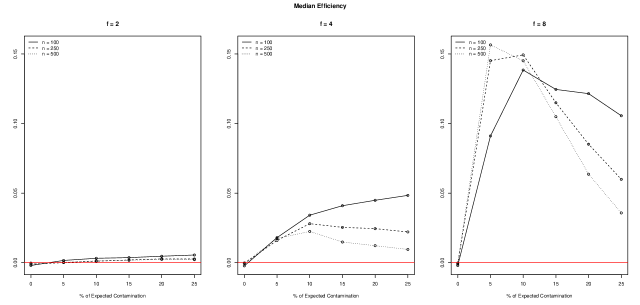
Figure 1: Median of Efficiencies for magnitude f = 2 (left), f = 4 (center) and f = 8 (right), $n_{d}$ = 100 (solid line), $n_{d}$ = 250 (dashed line) and $n_{d}$ = 500 (dotted line). We have the percentage of expected contamination in the x-axis and the median of efficiency in the y-axis.

To compare the model fitting we use the DIC as well as the CPO criteria. First, we define the relative DIC (RDIC) as

$$\mbox{RDIC}_{j}=\frac{\mbox{DIC}_{Gj}-\mbox{DIC}_{tj}}{\mbox{DIC}_{tj}},$$ (3.1)

for each one of the simulated data, $j=1,\ldots,1000$. In the top part of Figure 2 we plot the median of RDIC values obtained by the fitted Gaussian model and by fitted the Student’s t model for each scenario. From this Figure we observe the same pattern of Figure 1.

The summary statistic provided by the CPO criteria is called logarithm of the pseudo marginal likelihood (LPML) which evaluates the predictive power of a model. Therefore, to compare both models the LPML difference is used. To make it comparable to other goodness-of-fit measures, e.g. DIC, we define the -LPML by

$$\mbox{-LPML}_{j}=-\left(\sum_{i=1}^{n_{d}}\log\left\{\pi\left(y_{i}\mid\boldsymbol{y}_{-i}\right)\right\}\right)_{j}$$

where $j$ is the $j$-th dataset in a given scenario. In this definition, lower values of -LPML indicates better predictive power. In order to compare both approaches, we have computed the logarithm of the Pseudo Bayes Factor (lPsBF) (geiseddy1979) for each iteration. This measure is defined as

$$\mbox{lPsBF}_{j}=\mbox{-LPML}_{tj}-(\mbox{-LPML}_{Gj})=\mbox{LPML}_{Gj}-\mbox{LPML}_{tj}.$$

To make the comparison equivalent to the RDIC presented in Eq. (3.1) we define the relative lPsBF (RPsBF) as

$$\mbox{RPsBF}_{j}=\frac{\mbox{LPML}_{Gj}-\mbox{LPML}_{tj}}{\mbox{LPML}_{tj}}.$$

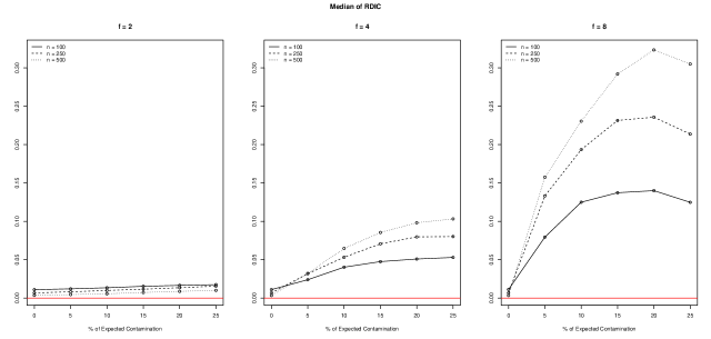
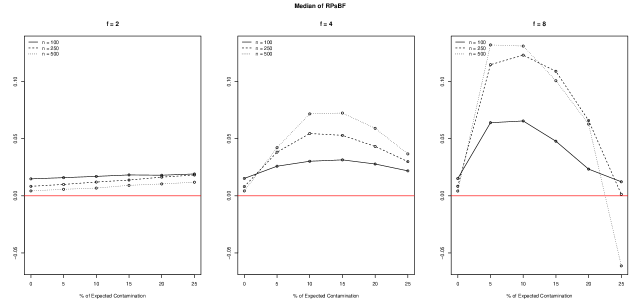
Figure 2: Top: Median of RDIC, in the y-axis, for all scenarios; Bottom: Median of RPsBF, in the y-axis, for all scenarios. We have the percentage of expected contamination in the x-axis and all scenarios are: f = 2 (left), f = 4 (center) and f = 8 (right), $n_{d}$ = 100 (solid line), $n_{d}$ = 250 (dashed line) and $n_{d}$ = 500 (dotted line).

From the bottom part of Figure 2, all conclusions from the MSE and RDIC can be applied in the context of the RPsBF measure, but the gain becomes more evident. Moreover, we can see from the bottom part of Figure 2 that when the simulated scenario is stable with low expected proportion and low contamination, the median of the RPsBF is small and not significant. However, for larger sample size and contamination it is showed that the Student-t approach is preferable for most of the scenarios and highlights this choice when the magnitude of the contamination increase reaching values of this median relative difference even higher than 10% in some cases. One curious fact observed is that in the most critical scenario where $p=0.25$, $f=8$ and $n_{d}=500$ the RPsBF values pointed incisively to the Gaussian approach, indicating that, since the generation process has too much contamination and generates to many innovative outliers, even the Student-t approach is not able to control for this behavior producing predictive measures that are less accurate.

From the simulation study we can conclude that the more flexible model is preferred over the traditional one in most of the scenarios analyzed, and the gap between the models are higher when a moderate number of innovative outliers are involved.

4 Data Application

The goal of this Section is to analyze Brazilian Homicide rates with approximate Bayesian Inference for Dynamic Models using R-INLA. The data comprises homicide rates of all the Brazilian cities available online in the database of the Brazilian National Public Health System (DATASUS). The time series under study represents the number of events standardized by each city population. In Brazil, experimental studies capable of evaluating the impact of determined political program about the spatial or temporal crime pattern are not common, mainly because of the difficulty in getting such data. On the other hand, international experience points-out that crime prevention policies are efficient after considering characteristics in which crime occurs (sherman1995; sherman1997; sherman1998).

According to Waiselfisz2012 and due to Brazilian legislation number 6,216 of 1975, all death, due to natural causes or not, must have a corresponding death register. This death register, made by a legist or two witnesses, has a standard national structure containing age, sex, civil state, occupation, naturality and local residence of the victim. According to the law, the death register must be computed by the ”local of the death”, i.e., the local of the occurrence of the event. All death occurrences in the dataset have been classified by the Brazilian government as homicides and comprises annual time series from 1980 to 2010.

Homicides studies have a broad field of sociological research (see, for example, jacobs2008). Homicides represent a specific criminal category that, although it has less cases when compared to patrimonial crimes, as burglary and robbery, it generates strong population demand for public policies of prevention. In this sense, studies that deal with the temporal dynamic of homicides try to associate, in a general way, this behavior with economic, social and political factors. For instance, high Brazilian homicide rates could be due to high levels of unemployment, poverty and economic inequality (mir2004). Population age structure (graham1995; floodpage2000) and disordered populational growth, or inequality in social conditions, could be other factors to explain these rates (blau1982). In summary, alteration in the criminal historic behavior is associated to law-enforcement elements, such as increase of the number of police officers, expenses with safety policies and increase of imprisonment rates. Analyzing data from New York City, zimring2007 concluded that ”there is a strong evidence that changing the number of cops, as well policing tactics, has a important impact in crime” (pg. 151). Specifically in Brazil, goertzel2009, while studying the behavior of the strong decline of homicides rates in São Paulo state since 2000’s, have concluded that more repressive police models and disarmament policies reduced substantially homicides and other violent crimes in the state. Statistically, it was expected that in certain regions, the rates could suffer from sudden structural changes. This fact requires a robust approach to model them, such as the assumption of heavy-tailed distribution for the latent system noise to handle possible innovative outliers as discussed in Section 3.

The model adopted was similar to Eqs. (2.6) and (2.7). However, to model each time series we considered the capital cities grouped according to a specific criterion. Specifically, we have used the following capital division:

• Group 1 (G1) - São Paulo and Rio de Janeiro

• Group 2 (G2) - Belo Horizonte, Recife, Vitória and Porto Alegre

• Group 3 (G3) - All the 21 remaining capitals.

This division was motivated in terms of different urbanization process. For each group created we have one tendency estimated for the capitals and one tendency estimated for all first order spatial neighbors (those which share border with the capital). Thus, for each group, there is a model for the capitals and another one for the capitals neighbors, totaling six models.

Let $Y_{til}$ be the Homicide Rate of city $i=1,\ldots,n_{l}$ in group $l=1,\ldots,6$ at time $t$, then we have the following model:

$$Y_{til} =a_{tl}+v_{til}, \,v_{til}\sim N(0,\theta_{1il}), t=1,...,31$$

$$a_{tl} =a_{(t-1)l}+w_{tl}, \,w_{tl}\sim(0,\theta_{2l}), t=2,...,31$$

where $w_{tl}$ is either Gaussian or Student-t and $n_{l}$ is the number of cities in group $l$.

To complete the model specification it is necessary to specify the priors for the hyperparameters. In our case, we have to specify priors for the precision of each group in the observational equation and a single prior for the system equation precision. The prior of the precision of the observational equation is created to cover with high probability the variances of all Brazilian cities, setting a prior $\theta_{1il}^{-1}\sim Gamma\left(5,500\right),i=1,\ldots,n_{l}$ and $l=1,\ldots,6$ we cover with 90% of probability the values between the 25th and 75th quantiles of the cities sample variance. For the precision prior for the latent equation, a prior $\theta_{2l}^{-1}\sim Gamma\left(1,0.1\right)$ is used for all cases. Finally, the same prior set in the simulation study for the degrees of freedom $\nu$ assuming 30% of probability of prior mass for $\nu$ values between 2 and 10 is used.

It is important to emphasize that the latent state represented by the vector $\boldsymbol{a}$, can be interpreted as the non-observed mean tendency of the cities of each modeling.

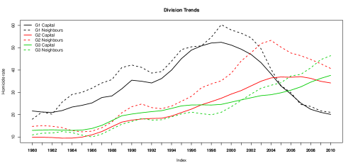
Figure 3: Division posterior tendencies, $\boldsymbol{a}$, for each group of Student-t approach. G1: São Paulo and Rio de Janeiro; G2: Belo Horizonte, Recife, Vitória and Porto Alegre; G3: All the 21 remaining capitals

To understand the temporal trends, sociological literature analyzes the context of how interpersonal violence spreads. Analyzing a historical time series of more than 30 years of delinquency and crime, shaw1942 verified that not only crime, but several social problems were related to a disorganized social environment. The theoretical approach developed by these authors helps to understand the effects of a unplanned urbanization process in criminal behavior. In Brazil, specially in big cities, the economic development was followed by the appearance of urban enclaves (such as slums) where the impairment of the traditional mechanisms of social control promotes an environment of differentiated criminal opportunities (sutherland1992). For more information about Social Disorganization Theory we refer to shaw1942 and kubrin2003.

Figure 3 presents the posterior tendency, $\boldsymbol{a}$, of each group capital and neighbours for the adjusted Student-t model. The tendency of the first group tells us that its urbanization process started earlier when compared to the other groups because the homicide rate started to get higher firstly. Another aspect was that until 2000, all the tendencies were nearly linear for all groups. However, a reverse tendency was observed as result of investments and criminal control policies established in G1 (goertzel2009). The other two groups are heading towards the same behavior, but they still didn’t show it in such an evident way, as seen in G1, the effect of safety policies. In G2 some states already adopted some safety measures, e.g., Minas Gerais, which capital is Belo Horizonte, with the creation of Integração da Gestão em Segurança Pública (IGESP) in May 2005, and Pernambuco, which capital is Recife, with the creation of the Pacto Pela Vida in May 2007.

		G1		G2		G3
		Gaussian	Student-t	Gaussian	Student-t	Gaussian	Student-t
-LPML	Capitals	229.09	227.81	496.72	496.45	2481.70	2473.55
	Neighbours	3536.78	3517.38	2379.98	2375.89	3026.54	3002.48
DIC	Capitals	460.22	459.64	997.44	996.60	4960.98	4946.32
	Neighbours	7063.15	7030.68	4753.67	4746.94	6040.70	6004.27

Table 1: Quality measures of the division. G1: São Paulo and Rio de Janeiro; G2: Belo Horizonte, Recife, Vitória and Porto Alegre; G3: All the 21 remaining capitals

In order to assess the goodness of fit of our robust approach, we computed the -LPMLs and the DICs for every model, as can be seen in Table 1. From Table 1, all criteria, -LPMLs and DICs, pointed to the robust approach assuming the Student-t distribution for the system noise. To verify the evidence that the robust approach outperforms significantly the traditional one, in the real data set, we chose to analyze Table 2 which was proposed and used in prates2010. From Table 2, we can see that the PsBF, which is the -LPML difference as presented in Section 3, have a positive evidence against the Gaussian model for the capital modeling in G1 (2PsBF = 2.56) and a strong evidence against the Gaussian model for the neighboring modeling in G2 (2PsBF = 8.18). However, the bigger gain in favor of the Student-t model is verified for the neighboring modeling in G1 and G3 as well as the capitals in this last group, with all having strong evidence in terms of the -LPML differences. Since for each group we have many first order neighbors time series, for G1, G2 and G3 there are 30, 24 and 152 neighbors respectively, analysis suggests that as the number of cities increases there is a demand for a more robust approach.

2PsBF	Evidence against Gaussian
(-1,1]	worth mention
(1,5]	positive
(5,9]	strong
(9,$\infty$)	very strong

Table 2: Pseudo Bayes Factor criteria

In our real data application the gain in terms of predictive power was very clear. We also should point out that there is evidence of deviation from Gaussianity when we look to the posterior distribution of the $\nu$ in the Student-t model. From Table 3 we can see the posterior median and 95% credible intervals (CI). The median measure indicates that the Student-t distribution is concentrated in medium values of the degrees of freedom but the 95% CI are highly asymmetric reaching very high values.

Group	Type	Median	95% Credible Interval
G1	Capitals	35.53	(5.84; 441.30)
	Neighbours	28.46	(6.04; 339.38)
G2	Capitals	39.93	(6.73; 533.77)
	Neighbours	31.69	(5.56; 445.12)
G3	Capitals	32.23	(5.14; 434.54)
	Neighbours	55.91	(21.69; 556.67)

Table 3: Posterior measures of the $\nu$ of Student-t approach. G1: São Paulo and Rio de Janeiro; G2: Belo Horizonte, Recife, Vitória and Porto Alegre; G3: All the 21 remaining capitals

5 Conclusions

This paper describes how to perform Bayesian inference using R-INLA to estimate non-Gaussian Dynamic Models when the evolution noise has a non-Gaussian distribution. Such models can be viewed as part of latent hierarchical models where a non-Gaussian Random Field is assumed for the latent field and, therefore, invalidates the direct use of the INLA methodology that requires that the latent field must be Gaussian.

Using a random walk example we presented how to use an augmented structure to overcome the Gaussian limitation of INLA for the latent field. The key to understand why our approach works relies on the fact that we approximate the non-Gaussian latent field through a Gaussian distribution and corrects this approximation in the likelihood function trying to minimize the loss of this approximation for dependent models. We discussed and explained the reasons to make this approximative approach and, specially, where in the R-INLA calculations it will impact.

Through simulations, we showed the necessity of more robust models when the time series suffer sudden structural changes. From our results we observe that Gaussian models are sensitive to structural changes while our approach assuming a Student-t field is robust. Specifically, our simulation study presented an incisive demand to avoid the usual Gaussian assumption in most contaminated scenarios. There are indication that some public policies for crime control can generate a positive effect in crime’s temporal tendencies allowing the presence of structural changes. It is evident that other control factors might help to confirm this hypothesis, however it is very likely that investments in security policies, such as those implemented in G1 and G2, have contribution in the dynamic observed. Our homicide rate application pointed-out, as expected, that public policies could play an important role to explain homicides dynamics through a robust approach due to the characteristic of these kind of data. Although we analyzed homicide rate because of their sociological impacts, we are aware that this extension would also be well justified in other fields such as stochastic volatility models (see, for example, jacquier2003).

As mentioned in Section 2 a natural extension of the model class presented is the DGLM, where one could assume a non-Gaussian distribution for the observed data and, consequently, impacting Eq. (2.5) which both $g_{t}(x_{t})$ and $h_{t}(x_{t})$ could have a non-quadratic form. This extension is investigated in a different manuscript. The main advantage of the model structure presented here is that it allows users to fit basically any complex structured non-Gaussian dynamic model with fast and good accuracy using a friendly tool already available.

We believe that the applied community can make good use of this methodology when necessary. For real time series data is not rare to observe structural breaks and a robust approach, as the one presented, may be more adequate to adjust this type of data. Furthermore, we have formalized how to use the R-INLA software for non-Gaussian dynamic models in a simple way.