The closure of a linear space in a product of lines

Abstract

Given a linear space $L$ in affine space $\mathbb{A}^{n}$, we study its closure $\widetilde{L}$ in the product of projective lines $(\mathbb{P}^{1})^{n}$. We show that the degree, multigraded Betti numbers, defining equations, and universal Gröbner basis of its defining ideal $I(\widetilde{L})$ are all combinatorially determined by the matroid $M$ of $L$. We also prove $I(\widetilde{L})$ and all of its initial ideals are Cohen-Macaulay with the same Betti numbers, and can be used to compute the $h$-vector of $M$. This variety $\widetilde{L}$ also gives rise to two new objects with interesting properties: the cocircuit polytope and the external activity complex of a matroid.

1 Introduction.

If $L\subset\mathbb{A}^{n}$ is a $d$-dimensional linear space in affine space $\mathbb{A}^{n}$ over an infinite field ${\mathbbm{k}}$, its usual closure in $\mathbb{P}^{n}$ is one of the simplest projective varieties. It is trivially a projective linear space, and its defining ideal is generated by $n-d$ linear forms. However, this is only one of many possible closures!

In this paper we study the next simplest possibility. Choose a frame $F=\{\langle e_{1}\rangle,\ldots,\langle e_{n}\rangle\}$ where the $e_{i}$ form a basis of $n$-space and $\langle\ \rangle$ denotes linear span. This frame gives rise to an embedding $\mathbb{A}^{n}\hookrightarrow(\mathbb{P}^{1})^{n}$, and we consider the closure $\widetilde{L}\subset(\mathbb{P}^{1})^{n}$ of $L$ in this product of projective lines. This case is already quite interesting; several algebraic, combinatorial, and geometric invariants of $\widetilde{L}$ are determined purely combinatorially. There is a matroid $M$ which encodes the relative position of $L$ with respect to the frame $F$. Our main result is that this matroid, which in principle only knows linear information about $L$, actually determines much of the structure of $\widetilde{L}$:

Theorem 1.1.

Let $L\subset\mathbb{A}^{n}$ be a linear space and let $\widetilde{L}$ be its closure via the embedding $\mathbb{A}^{n}\hookrightarrow(\mathbb{P}^{1})^{n}$. The following invariants depend only on the matroid of $L$: the $\mathbb{Z}^{n}$–multidegree of $\widetilde{L}$, the multigraded Betti numbers of $I(\widetilde{L})$ and all its initial ideals, the number of minimal generators of the defining ideal $I(\widetilde{L})$, and the set of initial ideals of $I(\widetilde{L})$. Furthermore, $I(\widetilde{L})$ and all of its initial ideals are Cohen-Macaulay with the same Betti numbers.

In fact, when we state this result more precisely in Theorem 1.3, we will see that several important matroid invariants are realized as algebro-geometric invariants of the projective variety $\widetilde{L}$. For instance, we can use $\widetilde{L}$ to compute algebraically the $h$-vector of the matroid of $L$, and the internal activities of its bases under any order. This variety also gives rise to two new objects with interesting properties: the cocircuit polytope and the external activity complex of a matroid.

The paper is organized as follows. In Section 1.1 we define our main subject of study: the closure of a linear space $L\subset\mathbb{A}^{n}$ in $(\mathbb{P}^{1})^{n}$. We state our main algebraic and combinatorial theorems in Sections 1.2 and Section 1.3 respectively, illustrating them in an example. Section 1.4 discusses related work. In Sections 2 and 3 we collect the basic facts from matroid theory and commutative algebra that we will need. In Section 4 and 5 respectively, we introduce and study two combinatorial objects that arise naturally in our work: the cocircuit polytope and the external activity complex of a matroid. We study their combinatorial properties, which may be interesting in their own right, but also play a key role in the proof of our main result, Theorem 1.3. We carry out this proof in Section 6. Finally, in Section 7 we extend our results to affine linear spaces. In that case the invariants of $\widetilde{L}$ are controlled by two matroids, and Las Vergnas’s Tutte polynomial of a morphism of matroids plays an interesting role.

1.1 Closures of linear spaces.

Choose a frame $F=\{\langle e_{1}\rangle,\ldots,\langle e_{n}\rangle\}$ where the $e_{i}$ form a basis of ${\mathbbm{k}}^{n}$ and $\langle\ \rangle$ denotes linear span. This allows us to identify $\mathbb{A}^{n}$ with $\mathbb{A}^{1}\times\cdots\times\mathbb{A}^{1}$. The usual embedding of $\mathbb{A}^{1}$ into $\mathbb{P}^{1}$ by adding a single point at infinity then gives us an embedding $\mathbb{A}^{n}\hookrightarrow(\mathbb{P}^{1})^{n}$.

Definition 1.2.

If $X$ is an affine variety in affine space $\mathbb{A}^{n}$, we let ${\widetilde{X}}$ denote the scheme-theoretic closure ${\widetilde{X}}$ of $X$ in $(\mathbb{P}^{1})^{n}$ induced by this embedding $\mathbb{A}^{n}\hookrightarrow(\mathbb{P}^{1})^{n}$. If $I=I(X)$ is the ideal of polynomials vanishing at $X$, we let $\widetilde{I}=I({\widetilde{X}})$ be the ideal of polynomials vanishing at ${\widetilde{X}}$.

For the remainder of the paper, we fix a choice of coordinates, and let $S={\mathbbm{k}}[x_{1},\ldots,x_{n}]$. The ideals $I(X)\subset S$ and $I(\widetilde{X})\subset{\mathbbm{k}}[x_{1},\ldots,x_{n},y_{1},\ldots,y_{n}]$ of ${\widetilde{X}}$ are related by

$$I(\widetilde{X}):=(f^{h}\ |\ f\in I),$$

where $f^{h}$ is the total homogenization of $f$, obtained by substituting $x_{i}$ with $x_{i}/y_{i}$ in $f$ and clearing denominators.

For general $X$, it does not suffice to only homogenize a set of generators of $I$ to cut out $\widetilde{X}$. It seems quite difficult to find a canonical presentation of the ideal $I(\widetilde{X})$, or to determine its algebraic invariants, such as the degree, number of generators, or multigraded Betti numbers. However, we show that when $X=L$ is a linear subspace (resp., an affine subspace), all of these questions have elegant answers in terms of the matroid of $L$ (resp., the morphism of matroids), which encodes the relative position of the subspace $L$ with respect to the chosen frame $F$. Let us describe this matroid in two ways.

Our linear space $L$ corresponds to a point in $\mathrm{Gr}(d,n)$, the Grassmannian of $d$-subspaces of ${\mathbbm{k}}^{n}$. The choice of a basis $\{e_{1},\ldots,e_{n}\}$ gives an embedding $\pi:\mathrm{Gr}(d,n)\to\mathbb{P}(\wedge^{d}{\mathbbm{k}}^{n})$ which maps a vector subspace $L$ of ${\mathbbm{k}}^{n}$ to its Plücker vector $\pi(L)$ in $\mathbb{P}(\wedge^{d}{\mathbbm{k}}^{n})$. Although the coordinates of $\pi(L)$ depend on the choice of basis, the set of coordinate hyperplanes containing $\pi(L)$ only depends on the frame $F$. This set can be identified with the matroid $M$ of $L$: for a $d$-subset $S$ of $[n]$, the hyperplane $H_{S}$ contains $\pi(L)$ if and only if $[n]-S$ is not a basis of $M$.

More explicitly, if $A$ is an $(n-d)\times n$ matrix whose rows generate the ideal $I=I(L)$ when regarded as linear forms, then the bases of the matroid $M$ are the linearly independent $(n-d)$-subsets of columns of $A$. This matroid will play a key role in what follows.

1.2 Our results on closures of linear spaces.

Given a linear space $L\subset\mathbb{A}^{n}$, we are interested in computing various invariants of the closure $\widetilde{L}\subset(\mathbb{P}^{1})^{n}$ and its ideal $I(\widetilde{L})\subset{\mathbbm{k}}[x_{1},\ldots,x_{n},y_{1},\ldots,y_{n}]$. We consider two gradings of ${\mathbbm{k}}[x_{1},\ldots,x_{n},y_{1},\ldots,y_{n}]$ which make the ideal $I(\widetilde{L})$ homogeneous: the bidegree with

$$\mathrm{bideg\,\,}x_{i}=(1,0),\qquad\mathrm{bideg\,\,}y_{i}=(0,1)\qquad(1\leq i\leq n)$$

and the $\mathbb{Z}^{n}$-multidegree given by

$$\mathrm{mdeg\,\,}x_{i}=\mathrm{mdeg\,\,}y_{i}=e_{i}\qquad(1\leq i\leq n)$$

where $e_{i}$ is the $i$th unit vector in $\mathbb{Z}^{n}$.

The following theorem shows that the structure of the matroid $M$ of $L$ determines several important geometric, algebraic, and combinatorial invariants of $I(\widetilde{L})$. Conversely, it offers a geometric context where Tutte’s basis activities and other matroid invariants appear very naturally. We will discuss in detail all the relevant definitions in Section 2.

Theorem 1.3.

Let $L\subset\mathbb{A}^{n}$ be a $d$-dimensional linear space and let ${\widetilde{L}}\subset(\mathbb{P}^{1})^{n}$ be the closure of $L$ induced by the embedding $\mathbb{A}^{n}\hookrightarrow(\mathbb{P}^{1})^{n}$. Let $M$ be the matroid of $L$; it has rank $r=n-d$. Then:

1. The homogenized cocircuits of $I(L)$ minimally generate the ideal $I(\widetilde{L})$.

2. The homogenized cocircuits of $I(L)$ form a universal Gröbner basis for $I(\widetilde{L})$, which is reduced under any term order.

3. The $\mathbb{Z}^{n}$-multidegree of $\widetilde{L}$ is $\sum\limits_{B}t_{b_{1}}\cdots t_{b_{r}}$ summing over all bases $B=\{b_{1},\ldots,b_{r}\}$ of $M$.

4. The bidegree of $\widetilde{L}$ is $t^{r}h_{M}(s/t)$ where $h_{M}$ is the $h$-polynomial of $M$.

5. There are at most $r!\cdot b$ distinct initial ideals of $I(\widetilde{L})$, where $b$ is the number of bases of $M$.

6. The initial ideal $\operatorname{in}_{<}I(\widetilde{L})$ is the Stanley–Reisner ideal of the external activity complex $B_{<}(M^{*})$ of the dual matroid $M^{*}$. Its primary decomposition is:

   $$\operatorname{in}_{<}I(\widetilde{L})=\bigcap_{B\textrm{ basis }}\left<\,x_{e}\,:\,e\in IA_{<}(B)\,,\,y_{e}\,:\,e\in IP_{<}(B)\right>$$

   where $B=IA_{<}(B)\,\sqcup\,IP_{<}(B)$ is the partition of $B$ into internally active and passive elements with respect to $<$.

Remark 1.4.

A remark is in order about Theorem 1.3(f). An initial ideal $\operatorname{in}_{<}I(\widetilde{L})$ is determined by a term order $<$ on ${\mathbbm{k}}[x_{1},\ldots,x_{n},y_{1},\ldots,y_{n}]$. In turn, $<$ leads to a linear order on $[n]$ which we also denote $<$, is defined by $i<j$ for $i,j\in[n]$ whenever $x_{i}y_{j}>x_{j}y_{i}$ (or, more revealingly, $x_{i}/y_{i}>x_{j}/y_{j}$) in the term order $<$. This is the linear order $<$ with respect to which $IA(B)$ and $IP(B)$ are defined.

We find it remarkable that the matroid $M$, which only contains linear information about $L$, determines so many invariants of the projective variety $\widetilde{L}$. Perhaps this becomes less surprising once we know (a) and (b), which tell us that the form of the defining equations for $\widetilde{L}$ is determined by the matroid. However, in our proof of (a) and (b), we rely on having already computed (using geometric and combinatorial arguments) the invariants of $\widetilde{L}$ and its degenerations in (c) and (f).

Theorem 1.5.

Let $L$ be a linear $d$-space in $\mathbb{A}^{n}$, and $I(\widetilde{L})$ the ideal of its closure in $(\mathbb{P}^{1})^{n}$. The non-zero multigraded Betti numbers of $S/I(\widetilde{L})$ are precisely:

$$\beta_{i,{\textbf{a}}}(S/I(\widetilde{L}))=|\mu(F,\widehat{1})|$$

for each flat $F$ of $M$, where $i=r-r(F)$, and ${\textbf{a}}=e_{[n]-F}$. Here $\mu$ is the Möbius function of the lattice of flats of $M$. Furthermore, all of the initial ideals have the same Betti numbers:

$$\beta_{i,{\textbf{a}}}(S/I(\widetilde{L}))=\beta_{i,{\textbf{a}}}(S/(\operatorname{in}_{<}I(\widetilde{L})))$$

for all a and for every term order $<$.

As a corollary we obtain the following result.

Theorem 1.6.

If $L$ is a linear space then the ideal $I(\widetilde{L})$ and all of its initial ideals are Cohen-Macaulay.

Before stating the relevant definitions in Section 2, we now briefly introduce them while we discuss an example in detail.

1.2.1 An example.

Example 1.7.

Let $L$ be the subspace of $\mathbb{A}^{6}$ cut out by the linear ideal

$$I=\left<x_{1}+x_{2}+x_{6},\,\,x_{2}-x_{3}+x_{5},\,\,x_{3}+x_{4}\right>.$$

This ideal is given by $r=3$ independent equations in $n=6$ variables, and the corresponding linear subspace $L$ has dimension $d=n-r=3$.

Consider the $r\times n$ matrix whose rows correspond to our 3 equations:

$$A=\begin{bmatrix}1&1&0&0&0&1\\ 0&1&-1&0&1&0\\ 0&0&1&1&0&0\end{bmatrix}.$$

We regard the columns of $A$ as a point configuration in $\mathbb{P}^{r-1}=\mathbb{P}^{2}$, respectively, as shown in Figure 1. The affine dependence relations among the points correspond to the linear dependence relations among the columns of the matrix. A different generating set for $I$ would give a different point configuration with the same affine dependence relations.

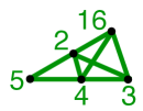
Figure 1: A point configuration $A\subset\mathbb{P}^{2}$ corresponding to the linear ideal $I$.

It is known [Stu96, Prop. 1.6] that the minimal universal Gröbner basis of $I$ is given by the cocircuits of $I$: the linear forms in $L$ using an inclusion-minimal set of variables.

$$I=\left<x_{1}+x_{2}+x_{6},\,\,x_{1}+x_{3}-x_{5}+x_{6},\,\,x_{1}-x_{4}-x_{5}+x_{6},\,\,x_{2}-x_{3}+x_{5},\,\,x_{2}+x_{4}+x_{5},\,\,x_{3}+x_{4}\right>$$

We identify the cocircuits with their support sets

$${\cal D}=\{126,\,\,1356,\,\,1456,\,\,235,\,\,245,\,\,34\}$$

They are the complements of the hyperplanes $345,24,23,146,136,$ and $1256$ spanned by subsets of $A$. Theorem 1.3(a,b) says that the homogenized cocircuits minimally generate $\widetilde{I}$, and give a universal Gröbner basis:

$$\widetilde{I}=\left<{\color[rgb]{0,0,1}x_{1}}y_{2}y_{6}+y_{1}{\color[rgb]{0,0,1}x_{2}}y_{6}+y_{1}y_{2}{\color[rgb]{0,0,1}x_{6}},\,\,{\color[rgb]{0,0,1}x_{1}}y_{3}y_{5}y_{6}+y_{1}{\color[rgb]{0,0,1}x_{3}}y_{5}y_{6}-y_{1}y_{3}{\color[rgb]{0,0,1}x_{5}}y_{6}+y_{1}y_{3}y_{5}{\color[rgb]{0,0,1}x_{6}},\ldots,\,{\color[rgb]{0,0,1}x_{3}}y_{4}+y_{3}{\color[rgb]{0,0,1}x_{4}}\right>.$$

The bases of $A$ are the maximal independent sets of $A$; they correspond to the non-zero maximal minors of $A$, and hence to the non-zero Plücker coordinates of $L$. In Figure 1 they correspond to triples of non-collinear points. The $13$ bases of $A$ are

$${\cal B}=\{123,124,134,135,145,234,235,236,245,246,346,356,456\}.$$

Theorem 1.3(c) then states that the multidegree of $\widetilde{L}$ is

$$\textrm{mdeg }\widetilde{L}=t_{1}t_{2}t_{3}+t_{1}t_{2}t_{4}+t_{1}t_{3}t_{4}+\cdots+t_{4}t_{5}t_{6}.$$

The $f$-vector $f=(1,6,14,13)$ counts the number $f_{i}$ of independent sets of size $i$ for $i=1,\ldots,r$. The $h$-polynomial is $h_{0}x^{r}+h_{1}x^{r-1}+\cdots+h_{r}x^{0}=f_{0}(x-1)^{r}+f_{1}(x-1)^{r-1}+\cdots+f_{r}(x-1)^{0}$; in this case it equals $x^{3}+3x^{2}+5x+4$. Thus Theorem 1.3(d) predicts that

$$\mathrm{bideg\,\,}\widetilde{L}=s^{3}+3s^{2}t+5st^{2}+4t^{3}.$$

Theorem 1.3(e) says that $I(\widetilde{L})$ has at most $(6-3)!\cdot 13=78$ initial ideals. Using the software Gfan [Jen] one can check that it actually has $72$ initial ideals.

Theorem 1.3(f) tells us the primary decomposition of the initial ideal $I_{<}=in_{<}I(\widetilde{L})$ with respect to any linear order $<$. If ${\color[rgb]{0,0,1}x_{1}}/y_{1}>\cdots>{\color[rgb]{0,0,1}x_{6}}/y_{6}$, which leads to the natural order $1<2<\cdots<6$ on the elements of the matroid, we get

$$I_{<} = \left<{\color[rgb]{0,0,1}x_{1}}y_{2}y_{6},\,\,{\color[rgb]{0,0,1}x_{1}}y_{3}y_{5}y_{6},\,\,{\color[rgb]{0,0,1}x_{1}}y_{4}y_{5}y_{6},\,\,{\color[rgb]{0,0,1}x_{2}}y_{3}y_{5},\,\,{\color[rgb]{0,0,1}x_{2}}y_{4}y_{5},\,\,{\color[rgb]{0,0,1}x_{3}}y_{4}\right>$$

$$= \left<{\color[rgb]{0,0,1}x_{1}},{\color[rgb]{0,0,1}x_{2}},{\color[rgb]{0,0,1}x_{3}}\right>\,\cap\,\left<{\color[rgb]{0,0,1}x_{1}},{\color[rgb]{0,0,1}x_{2}},y_{4}\right>\,\cap\,\left<{\color[rgb]{0,0,1}x_{1}},y_{3},y_{4}\right>\,\cap\,\left<{\color[rgb]{0,0,1}x_{1}},{\color[rgb]{0,0,1}x_{3}},y_{5}\right>\,\cap\,\left<{\color[rgb]{0,0,1}x_{1}},y_{4},y_{5}\right>\,\cap\,$$

$$\left<y_{2},y_{3},y_{4}\right>\,\cap\,\left<y_{2},{\color[rgb]{0,0,1}x_{3}},y_{5}\right>\,\cap\,\left<x_{2},{\color[rgb]{0,0,1}x_{3}},y_{6}\right>\,\cap\,\left<y_{2},y_{4},y_{5}\right>\,\cap\,\left<{\color[rgb]{0,0,1}x_{2}},y_{4},y_{6}\right>\,\cap\,$$

$$\left<y_{3},y_{4},y_{6}\right>\,\cap\,\left<{\color[rgb]{0,0,1}x_{3}},y_{5},y_{6}\right>\,\cap\,\left<y_{4},y_{5},y_{6}\right>.$$

We have a primary component $\left<z_{b}\,:\,b\in B\right>$ for each basis $B$, where $z_{b}$ equals ${\color[rgb]{0,0,1}x_{b}}$ or $y_{b}$ depending on whether $b$ is internally active or passive in $B$. For each $b\in B$ consider the cocircuit $D(B,b)$, which consists of the points not on the hyperplane spanned by $B-b$. If $b$ is the smallest element of $D(B,b)$ then $b$ is said to be active in $B$, and $z_{b}={\color[rgb]{0,0,1}x_{b}}$. Otherwise, $b$ is passive in $B$ and $z_{b}=y_{b}$.

For example, the basis $235$ contributes the primary component $\left<y_{2},{\color[rgb]{0,0,1}x_{3}},y_{5}\right>$ because $2$ is internally passive ($2$ is not the smallest element in $D(235,2)=126$), $3$ is internally active ($3$ is smallest in $D(235,3)=34$), and $5$ is internally passive ($5$ is not smallest in $D(235,5)=1456)$.

Note that, from the primary decomposition of $I_{<}$ above, we can read off the multidegree and bidegree immediately. Each component contributes a monomial, where terms ${\color[rgb]{0,0,1}x_{i}}$ and $y_{i}$ respectively contribute factors of $s$ and $t$ to the bidegree, and a factor of $t_{i}$ to the multidegree. Therefore, if one is able to compute this primary decomposition, one immediately gets the list of bases and the $h$-polynomial of the matroid. From this point of view, it is surprising that when we choose different orders $<$ we get the same bidegree.

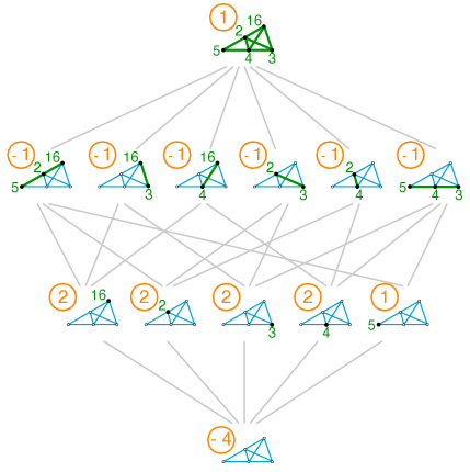
Figure 2: The Möbius function $\mu(F,\widehat{1})$ of the lattice of flats $M$ encodes the non-zero multigraded Betti numbers of $I(\widetilde{L})$.

Theorem 1.5 is best understood pictorially. The flats of $M$ are the affine subspaces spanned by the points in $A$. They are partially ordered by inclusion. Recursively define the numbers $\mu(F,\widehat{1})$ by $\mu(\widehat{1},\widehat{1})=1$ and $\mu(F,\widehat{1})=-\sum_{G>F}\mu(G,\widehat{1})$ for $G\neq\widehat{1}$, where $\widehat{1}$ is the maximal flat. These numbers are shown circled in Figure 2, and they give the non-zero multigraded Betti numbers of $S/I$:

$$\beta_{0,\mathbf{\emptyset}}=1$$

$$\beta_{1,\bf{34}}=\beta_{1,\bf{245}}=\beta_{1,\bf{235}}=\beta_{1,\bf{1456}}=\beta_{1,\bf{1356}}=\beta_{1,\bf{126}}=1$$

$$\beta_{2,\bf{2345}}=\beta_{2,\bf{13456}}=\beta_{2,\bf{12456}}=\beta_{2,\bf{12356}}=2,\qquad\beta_{2,\bf{12346}}=1$$

$$\beta_{3,\bf{123456}}=4$$

From this we can immediately read off the Betti numbers

$$\beta_{0}=1,\quad\beta_{1}=6,\quad\beta_{2}=9,\quad\beta_{3}=4$$

of $S/I$, as well as the standard $\mathbb{Z}$-graded Betti table of $S/I$, whose $(i,j)$ entry is $\beta_{i,i+j}=\sum\limits_{|{\textbf{a}}|=i+j}\beta_{i,{\textbf{a}}}$:

$$\begin{array}[]{c|cccc}I&1&6&9&4\\ \hline\cr&1&-&-&-\\ &-&1&-&-\\ &-&3&2&-\\ &-&2&7&4\end{array}$$

In view of Theorem 1.3(b), the equality for $i=1$ in Theorem 1.5 follows from the fact that $I(\widetilde{L})$ is robust; that is, it is minimally generated by a universal Gröbner basis. For example, the Betti number $\beta_{1,\mathbf{34}}=1$ corresponds to the generator ${\color[rgb]{0,0,1}x_{3}}y_{4}+y_{3}{\color[rgb]{0,0,1}x_{4}}$ of $\widetilde{I}$.

All of these results have generalizations to affine subspaces of $\mathbb{A}^{n}$. We delay the precise statements and proofs until Section 7.

1.3 Our results on matroids.

Our analysis of the closure $\widetilde{L}$ of a linear space $L\subset\mathbb{A}^{n}$ in $(\mathbb{P}^{1})^{n}$ gives rise to some constructions and results in matroid theory of independent interest.

Fix a basis $e_{1},\ldots,e_{n}$ of $\mathbb{R}^{n}$ and let $\Delta=\mathrm{conv}\{e_{1},\ldots,e_{n}\}$ be the standard simplex in $\mathbb{R}^{n}$. For each subset $S\subseteq[n]$ consider the indicator vector $e_{S}=\sum_{s\in S}e_{s}$ and the face $\Delta_{S}=\mathrm{conv}\{e_{s}\,:\,s\in S\}$ of $\Delta$. For a matroid $M$ on $[n]$ consider the cocircuit polytope

$$O_{M}=\sum_{D\textrm{ cocircuit of }M}\Delta_{D},$$

where the Minkowski sum of $P,Q\subset\mathbb{R}^{n}$ is $P+Q:=\{p+q\,:\,p\in P,q\in Q\}$.

Theorem 1.8.

If a matroid $M$ on $[n]$ has rank $r$, then the cocircuit polytope $O_{M}$

1. is given by the equation $\sum_{i=1}^{n}x_{i}=D([n])$ and the inequalities $\sum_{i\in S}x_{i}\leq D(S)\textrm{ for }S\subseteq[n]$, where $D(S)$ is the number of cocircuits intersecting $S$,

2. has dimension $n-c$ where $c$ is the number of connected components of $M$,

3. has the matroid polytope $P_{M}=\mathrm{conv}\{e_{B}\,:\,B\textrm{ basis}\}$ as a Minkowski summand,

4. has at most $r!\cdot b$ vertices, where $b$ is the number of bases.

We are also led to the study of an interesting simplicial complex, which we call the external activity complex. Let $M$ be a matroid and let $<$ be a linear order on the ground set $S$. Consider the $2|E|$-element set $\{x_{e},y_{e}\,:\,e\in E\}$, and identify subsets and monomials, and write

$$x_{A}y_{B}:=\{x_{a}\,:a\in A\}\cup\{y_{b}\,:\,b\in B\}.$$

Every basis $B$ of $M$ gives rise to a partition of $[n]-B$ into the sets $EA_{<}(B)$ and $EP_{<}(B)$ of externally active and passive elements. These sets, which will be defined in Section 2, are similar and related to the sets $IA_{<}(B)$ and $IP_{<}(B)$ of Theorem 1.3(e).

Theorem 1.9.

Let $M$ be a matroid and $<$ a linear order on its ground set. There is a simplicial complex $B_{<}(M)$ on $\{x_{e},y_{e}\,:\,e\in E\}$, called the external activity complex, such that

1. The minimal non-faces are $x_{\min C}y_{C-\min C}$ for each circuit $C$.

2. The facets of $B_{<}(M)$ are the sets $x_{B\cup EP(B)}y_{B\cup EA(B)}$ for each basis $B$.

1.4 Motivation and related results.

The closures we study are similar to the reciprocal varieties of linear spaces considered in [PS06]. A reciprocal variety may be thought of as the closure arising from the homogenization $x_{i}\mapsto 1/y_{i}$. Proudfoot and Speyer proved that the reciprocal variety $L^{\perp}$ of a linear space has a universal Gröbner basis defined by circuit polynomials. They also proved that its degree can be computed in terms of the Tutte polynomial evaluated at $(1,0)$. In one sense, our results can be viewed as a proper homogenization of the reciprocal variety. Indeed, upon setting $x_{i}=1$ we obtain precisely the equations obtained in [PS06]. Upon substitution the minimality of the generators is not preserved, nor is the property that all monomial degenerations have the same Betti numbers. The bidegree of $I(\widetilde{L})$ is a homogenised $h$-polynomial whereas the degree of the reciprocal variety is equal to the constant term $h(0)$. Thus it seems that the added homogeneity enjoyed by the closure in $(\mathbb{P}^{1})^{n}$ captures more of the matroid structure.

We originally became interested in closures of linear spaces because of this universal Gröbner basis property and a well-known result for toric ideals: If $X$ is any affine toric variety, then its closure $\widetilde{X}$ in $(\mathbb{P}^{1})^{n}$ is called the Lawrence lifting of $X$. If $X$ is toric then $I(\widetilde{X})$ is minimally generated by a universal Gröbner basis (see [Stu96]). In general, we wanted an answer to the following

Question 1.10.

If $X\subset\mathbb{A}^{n}$ is a variety, and $I(\widetilde{X})$ is the ideal of its closure in $(\mathbb{P}^{1})^{n}$, when does

$$\beta_{i}(S/I(\widetilde{X}))=\beta_{i}(S/\operatorname{in}_{<}I(\widetilde{X}))\mbox{ for all $<$ }?$$

Sturmfels’ result says that equality holds if $X$ is defined by a toric ideal and $i=1$, and our result says that if $L$ is a linear space then equality holds for all $i$.

Originally we hoped that such a result might hold more generally, but little is true. Even for toric ideals, the question has a negative answer if $i\geq 2$ and the following example shows that even for $i=1$ the situation is quite subtle. This example also illustrates that, contrary to the case of closures in $\mathbb{P}^{n}$, there is no simple numerical relationship between the number of generators of $I(X)$ and $I(\widetilde{X})$, even in terms of Gröbner bases.

Example 1.11.

Let $I=I(X)=(x_{1}+x_{2}+x_{3},\,\,x_{1}+x_{3}+x_{4},\,\,x_{1}^{2}+x_{2}^{2}+x_{1}x_{4})$

$$\begin{array}[]{|r|ll|}\hline\cr&I(X)&I(\widetilde{X})\\ \hline\cr\mbox{number of generators}&3&12\\ \mbox{size of a reduced Gr\"{o}bner basis}&3&14\mbox{ or }15\\ \mbox{size of a universal Gr\"{o}bner basis}&8&21\\ \hline\cr\end{array}$$

The closures we study also arise in work of Aholt, Sturmfels, and Thomas [AST13] where they study maps induced by products of linear projections $V\to V/V_{i}$ when $\dim V=4$. Recently, Li has extended the results of [AST13] to arbitrary vector spaces. In [Li13] he computes the defining ideal and multi-degree for the closure of the image of such maps and proves that they are determined combinatorially.

Ideals minimally generated by universal Gröbner bases, called robust ideals in [BR13], are by no means a common occurrence. Even in the toric case, this condition is very strong, yet a complete classification is unknown. Nonetheless, robust ideals have cropped up in many classical situations; see [Boo12, BR13, CNG13, CHT06, PS06, SZ93].

2 Preliminaries from matroid theory.

The toolkit of matroid theory is ideally suited to study the geometric and algebraic invariants in this project. Matroid theory can be approached from many equivalent points of view. This can make the theory confusing at first, as different papers often use very different definitions of a matroid. However, in the long run, the existence of these “cryptomorphic” definitions is an extremely powerful feature of the theory. This project illustrates this point very well; many different matroid theoretic concepts appear naturally, as Example 1.7 shows. In this section we introduce these concepts in more detail; they will play a fundamental role in what follows. For a more thorough introduction, see [Bjö92, Oxl92].

2.1 One definition of a matroid.

Definition 2.1.

A matroid $M=(E,\mathcal{I})$ consists of a ground set $E$ and a family $\mathcal{I}$ of sets of $E$, called the independent sets of $M$, which satisfy the following axioms:

(I1) The empty set is independent.

(I2) A subset of an independent set is independent.

(I3) If $X$ and $Y$ are independent and $|X|<|Y|$, then there exists $y\in Y-X$ such that $X\cup y$ is independent.

Matroid theory can be thought of as a combinatorial theory of independence. The prototypical example is the family of linear or realizable matroids, which arise from linear independence. If $E$ is a set of vectors in a vector space $V$, then the linearly independent subsets of $E$ form a matroid.

In a matroid $M$, a circuit is a minimal dependent set. A basis is a maximal independent set. All bases of $M$ have the same size, which is called the rank $r(M)$ of $M$. Similarly, all maximal independent subsets of any set $S\subseteq E$ have the same size, which is called the rank $r(S)$. There are equivalent definitions of matroids in terms of circuits, bases, and rank functions, among others.

In our running Example 1.7, the bases and circuits are:

$${\cal B} = \{123,124,134,135,145,234,235,236,245,246,346,356,456\},$$

$${\cal C} = \{16,125,256,345,1234,2346\}.$$

The independent sets are the subsets of the bases.

2.2 The $f$-vector, $h$-vector, and Tutte polynomial.

The $f$-vector $f_{M}=(f_{0},\ldots,f_{r})$ of a matroid $M$ records the number $f_{i}$ of independent sets of size $i$ for $0\leq i\leq r$. This information is equivalently recorded in the $h$-polynomial

$$h_{M}(x)=h_{0}x^{r}+h_{1}x^{r-1}+\cdots+h_{r}x^{0}=f_{0}(x-1)^{r}+f_{1}(x-1)^{r-1}+\cdots+f_{r}(x-1)^{0}.$$

The reverse polynomial $h_{r}x^{r}+\cdots+h_{0}$ is known as the shelling polynomial of $M$. The vector $h_{M}=(h_{0},\ldots,h_{r})$ is called the $h$-vector of $M$.

In our running Example 1.7 we already saw that there are 13 bases. All sets of size 0, 1, and 2 are independent except for the pair 16, so the $f$-vector is $(1,6,14,13)$. The $h$-polynomial is then

$$h_{M}(x)=(x-1)^{3}+6(x-1)^{2}+14(x-1)+13=x^{3}+3x^{2}+5x+4.$$

The $h$-polynomial is an evaluation of the most important enumerative invariant of a matroid, the Tutte polynomial:

$$T_{M}(x,y)=\sum_{A\subseteq E}(x-1)^{r-r(A)}(y-1)^{|A|-r(A)}.$$

A straightforward computation shows that

$$h_{M}(x)=T_{M}(x,1).$$

2.3 Duality and minors.

If ${\cal B}$ is the collection of bases of a matroid $M$ on $E$, then ${\cal B}^{*}:=\{E-B\,:\,B\in{\cal B}\}$ is also the collection of bases of a matroid, called the dual matroid $M^{*}$. If $M$ is the matroid of a set $A$ of $n$ vectors which generate ${\mathbbm{k}}^{d}$, then one can find a set of $n$ vectors which generate ${\mathbbm{k}}^{n-d}$ whose matroid is $M^{*}$. Figure 3 shows a point configuration dual to the one of Example 1.7. The reader may check that the bases of $A^{*}$ are precisely the complements of the bases of $A$.

A circuit of $M^{*}$ is called a cocircuit of $M$. It can also be characterized as a minimal set $D$ whose removal decreases the rank of $M$; i.e., $r(E-D)<r$. The cocircuits of $A$ in Example 1.7 are

$${\cal D}=\{34,126,235,245,1356,1456\}.$$

They are the complements of the hyperplanes spanned by subsets of $A$. In $A^{*}$ they are the circuits.

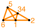
Figure 3: The point configuration $A\subset\mathbb{P}^{r-1}=\mathbb{P}^{2}$ and a dual configuration $A^{*}\subset\mathbb{P}^{n-r-1}=\mathbb{P}^{2}$.

The following technical lemma will be very useful to us.

Lemma 2.2.

[Oxl92] If $C$ is a circuit and $D$ is a cocircuit of $M$, then $|C\cap D|\neq 1$.

If $M$ is a matroid on $E$ and $A\subset E$ then there are matroids $M\backslash A=M|_{E-A}$ and $M/A$ on $E-A$, called the deletion and contraction of $A$ in $M$, whose independent sets are

$${\mathcal{I}}(M\backslash A) = \{I\in{\mathcal{I}}(M)\,:\,I\subseteq E-A\}$$

$${\mathcal{I}}(M/A) = \{I-B_{A}\,:I\in{\mathcal{I}}(M),B_{A}\subseteq I\}$$

where $B_{A}$ is a basis of $A$. Any sequence of deletions and contractions commutes. A minor of $M$ is any matroid obtained from $M$ by deletions and contractions.

Deletion and contraction are dual operations:

$$(M/A)^{*}=M^{*}\backslash A.$$

If $M$ comes from a set $S$ of vectors in a vector space $V$, then $M\backslash A$ corresponds to deleting the vectors in $A$, while $M/A$ corresponds to the images of those vectors in $V/\textrm{span}(A)$.

2.4 The matroid of a linear ideal.

Fix a choice of a standard basis for ${\mathbbm{k}}^{n}$. Let $L$ be an $r$-dimensional linear subspace of ${\mathbbm{k}}^{n}$ and let $I(L)\subset{\mathbbm{k}}[x_{1},\ldots,x_{n}]$ be its defining linear ideal. There is one particularly useful generating set for $I(L)$, which we now describe. For each linear form $f$ in $I(L)$ consider its support $\mathrm{supp}(f)\subseteq[n]$ consisting of those $i$ such that $x_{i}$ has a nonzero coefficient in $f$. Among these, consider the set ${\cal D}$ of inclusion-minimal supports; these are called the cocircuits of $I(L)$. They are the cocircuits of a matroid $M(L)$, called the matroid of $L$. Notice that for each cocircuit $D$ there is a unique linear form $f$ (up to scalar multiplication) in $I(L)$ with $\mathrm{supp}(f)=D$, so there is no ambiguity in calling this form $f$ a cocircuit as well.

Proposition 2.3.

[Stu96, Prop. 1.6] The cocircuits of the linear ideal $I(L)$ form a universal Gröbner basis for $I(L)$.

Linear matroids are precisely the matroids of linear ideals. As we explained in Example 1.7, if $B$ is a matrix whose rows generate $I(L)$, one may easily check that the linear matroid on the columns of $B$ equals the matroid of $L$.

Matroid duality can then be seen as a generalization of duality of subspaces. Our chosen basis for ${\mathbbm{k}}^{n}$ determines a dual basis for the dual vector space $({\mathbbm{k}}^{n})^{*}$. If $L^{\perp}\subset({\mathbbm{k}}^{n})^{*}$ is the orthogonal complement of our vector space $L$, then the matroid of $L^{\perp}$ is dual to the matroid of $L$.

2.5 Basis activities.

Proposition 2.4.

[Cra69] Given a basis $B$ and an element $x\notin B$, there is a unique circuit $C=C(B,x)$ contained in $B\cup x$. It is called the fundamental circuit of $B$ and $x$, and is given by:

$$C(B,x)=\{y\in E\,:\,(B\cup x)-y\textrm{ is a basis}\}$$

Notice that $x\in C(B,x)$.

Given a basis $B$ and an element $y\in B$, there is a unique cocircuit $D=D(B,y)$ contained in $E-B\cup y$. It is called the fundamental cocircuit of $B$ and $y$, and is given by:

$$D(B,y)=\{x\in E\,:\,(B-y)\cup x\textrm{ is a basis}\}$$

Notice that $y\in D(B,y)$.

Consider a linear order $<$ on the ground set of $M$. Let $B$ be a basis of $M$. We say that an element $e\notin B$ is externally active if it is the smallest element in $C(B,e)$, and it is externally passive otherwise. Let $EA_{<}(B)$ and $EP_{<}(B)$ be the sets of externally active and externally passive elements with respect to $B$ and $<$.

Similarly, we say that an element $i\in B$ is internally active if it is the smallest element in $D(B,i)$, and it is internally passive otherwise. We write $IA_{<}(B)$ and $IP_{<}(B)$ for the sets of internally active and internally passive elements with respect to $B$ and $<$. Notice that matroid duality reverses internal and external activity: $IA_{M,<}(B)=EA_{M^{*},<}([n]-B)$ and $IP_{M,<}(B)=EP_{M^{*},<}([n]-B)$.

We will need the following result by Crapo:

Theorem 2.5.

[Cra69] Let $M$ be a matroid on the ground set $S$ and let $<$ be a linear order on $S$. Every subset $A$ of $S$ can be uniquely written in the form $A=B\cup E-I$ for some basis $B$, some subset $E\subseteq EA(B)$, and some subset $I\subseteq IA(B)$. Equivalently, the intervals $[B-IA(B),B\cup EA(B)]$ form a partition of the poset $2^{S}$ of subsets of $S$ ordered by inclusion.

This can be used to prove:

Theorem 2.6.

[Cra69] Let $M$ be a matroid on the ground set $S$ and let $<$ be a linear order on $S$. Then the Tutte polynomial and $h$-polynomial of $M$ are given by

$$T_{M}(x,y)=\sum_{B\,\textrm{basis}}x^{|IA_{<}(B)|}y^{|EA_{<}(B)|},\qquad h_{M}(x)=\sum_{B\,\textrm{basis}}x^{|IA_{<}(B)|}.$$

This beautiful result implies, in particular, the nontrivial fact that the right hand side of each equation does not depend on the chosen linear order.

2.6 Lattice of flats and Möbius function.

A flat $F$ of a matroid $M$ is a subset which is maximal for its rank; that is, a set such that $r(F\cup f)=r(F)+1$ for all $f\notin F$. The flats of rank $r-1$ are called hyperplanes. In the case that interests us, when $M$ is the linear matroid of a set of vectors $E\subset{\mathbbm{k}}^{n}$, the flats of $M$ correspond to the subspaces spanned by subsets of $E$. The lattice of flats $L_{M}$ is the poset of flats ordered by containment; it is in fact a lattice, graded by rank. The flats in Example 1.7 are

$$L_{M}=\{\emptyset,16,2,3,4,5,1256,136,146,23,24,345,123456\},$$

as illustrated in Figure 2.

The Möbius function of $L_{M}$ is the map $\mu:Int(L_{M})\rightarrow\mathbb{Z}$ from the intervals of $L_{M}$ to $\mathbb{Z}$ characterized by $\mu(x,x)=1$ for all $x\in L_{M}$ and $\sum_{x\leq z\leq y}\mu(z,y)=0$ for all $x<y$. The Möbius number of $M$ is $\mu(M)=\mu(\widehat{0},\widehat{1})$, where $\widehat{0}$ and $\widehat{1}$ are the minimum and maximum elements of $L_{M}$. Figure 2 shows the value of $\mu(F,\widehat{1})$ next to each flat $F$ of $M$.

2.7 Independence complexes and cocircuit ideals.

To a matroid $M$ on the ground set $E$ one associates a simplicial complex

$$IN(M)=\{I\subseteq E\,:\,I\textrm{ is independent in }M\}$$

called the independence complex of $M$. For us, the independence complex of the dual matroid $M^{*}$ is more relevant. These complexes have very simple topology:

Theorem 2.7.

[Bjö92, Theorem 7.8.1] If $M$ is a matroid of rank $r$ on $[n]$, then

$$H_{i}(IN(M^{*});\mathbb{Z})=\begin{cases}\mathbb{Z}^{\,|{\mu}(M)|},&\mbox{if }i=n-r-1\mbox{ and $M$ has no loops}\\ 0,&\mbox{otherwise}.\end{cases}.$$

Recall that the Stanley-Reisner ideal of a simplicial complex $\Delta$ on a set $\{x_{1},\ldots,x_{n}\}$ is the ideal

$$I_{\Delta}=\left<x_{i_{1}}x_{i_{2}}\cdots x_{i_{k}}\,:\,\{i_{1},\ldots,i_{k}\}\textrm{ is not a face of }\Delta\right>\subset{\mathbbm{k}}[x_{1},\ldots,x_{n}].$$

The Stanley-Reisner ring is ${\mathbbm{k}}[x_{1},\ldots,x_{n}]/I_{\Delta}$. Since the minimal non-faces of $IN(M^{*})$ are the circuits of $M^{*}$, which are the cocircuits of $M$, the Stanley–Reisner ideal of $IN(M^{*})$ is the cocircuit ideal

$$I_{IN(M^{*})}=\left<\prod_{c\in C}x_{c}\,:C\textrm{ is a cocircuit of }M\right>.$$

The components of the primary decomposition of a squarefree monomial ideal $I_{\Delta}$ are in bijection with the facets of $\Delta$; each facet $F$ corresponds to the primary component $\left<x_{f}\,:\,f\notin F\right>$. [MS05, Theorem 1.7] Since the facets of $IN(M^{*})$ are the bases of $M^{*}$, we get that the primary decomposition of $I_{IN(M^{*})}$ is

$$I_{IN(M^{*})}=\bigcap_{B\textrm{ basis}}\left<x_{b}\,:\,b\in B\right>.$$

In our running Example 1.7 we have

$$I_{IN(M^{*})} = \left<x_{1}x_{2}x_{6},\,\,x_{2}x_{3}x_{5},\,\,x_{2}x_{4}x_{5},\,\,x_{3}x_{4},\,\,x_{1}x_{3}x_{5}x_{6},\,\,x_{1}x_{4}x_{5}x_{6}\right>$$

$$= \left<x_{1},x_{2},x_{3}\right>\,\cap\,\left<x_{1},x_{2},x_{4}\right>\,\cap\,\left<x_{1},x_{3},x_{4}\right>\,\cap\,\left<x_{1},x_{3},x_{5}\right>\,\cap\,\left<x_{1},x_{4},x_{5}\right>\,\cap\,$$

$$\left<x_{2},x_{3},x_{4}\right>\,\cap\,\left<x_{2},x_{3},x_{5}\right>\,\cap\,\left<x_{2},x_{3},x_{6}\right>\,\cap\,\left<x_{2},x_{4},x_{5}\right>\,\cap\,\left<x_{2},x_{4},x_{6}\right>\,\cap\,$$

$$\left<x_{3},x_{4},x_{6}\right>\,\cap\,\left<x_{3},x_{5},x_{6}\right>\,\cap\,\left<x_{4},x_{5},x_{6}\right>.$$

Now we recall Hochster’s formula for the Betti numbers of a squarefree monomial ideal:

Theorem 2.8.

[MS05, Corollary 5.12] The nonzero Betti numbers of the Stanley–Reisner ring $I_{\Delta}$ lie only in squarefree degrees $\sigma$, and

$$\beta_{i-1,\sigma}(I_{\Delta})=\dim_{\mathbbm{k}}\widetilde{H}^{|\sigma|-i-1}(\Delta|_{\sigma}).$$

Let us apply this formula to $\Delta=IN(M^{*})$ and $\sigma=E-A$ for a subset $A\subset E$. We have that $\Delta|_{E-A}=IN(M^{*}|_{E-A})=IN(M^{*}\backslash A)$. Notice that $(M^{*}\backslash A)^{*}=M/A$ has no loops if and only if $A$ is a flat of $M$. Also $r(M/A)=r-r(A)$ and $\mu(M/A)=\mu(A,\widehat{1})$. Combining these observations with Theorem 2.7, we obtain the following result.

Theorem 2.9.

The only nonzero Betti numbers of the cocircuit ideal $I_{IN(M^{*})}$ of $M$ are

$$\beta_{r-r(A)-1,e_{E-A}}(I_{IN(M^{*})})=|\mu(A,\widehat{1})|$$

for the flats $A$ of $M$.

3 Preliminaries from commutative algebra.

In this section we briefly review relevant definitions and results from combinatorial commutative algebra. We refer the reader to [HH11, MS05] for a thorough treatment of all of these topics.

3.1 Free resolutions and Betti numbers.

Recall that $S={\mathbbm{k}}[x_{1},\ldots,x_{n}]$. Let $M$ be a graded $S$-module. One important invariant of $M$ is its minimal free resolution, which is an exact sequence of maps of $S$-modules

where the $F_{i}$ are free modules chosen to have rank as small as possible. Such a resolution is unique up to isomorphism, and the maps can be chosen so that they are homogeneous with respect to the grading. Each $F_{i}$ is a direct sum

$$F_{i}=\bigoplus_{\mathbf{a}}S(-\mathbf{a})^{\beta_{i,\mathbf{a}}}$$

where $S(-\mathbf{a})$ denotes the free module whose generator lies in degree $\mathbf{a}$. The ranks of these graded pieces are defined to be the graded Betti numbers $\beta_{i,\mathbf{a}}$ and can be computed as dimensions of $\mathrm{Tor}$ modules according to the formula

$$\beta_{i,\mathbf{a}}(M)=\dim_{k}(\mathrm{Tor}^{S}_{i}(M,{\mathbbm{k}}))_{\mathbf{a}}.$$

The modules $F_{i}$ in the minimal free resolution are collectively called syzygies and encode algebraic relations among the generators of $M$. In what follows we assume that $M=S/I$ for a homogeneous ideal $I$.

Example 3.1.

With this notation, the ideal $\widetilde{I}$ in Example 1.7 has minimal free resolution

$$\lx@xy@svg{\hbox{\raise 0.0pt\hbox{\kern 5.5pt\hbox{\ignorespaces\ignorespaces\ignorespaces\hbox{\vtop{\kern 0.0pt\offinterlineskip\halign{\entry@#!@&&\entry@@#!@\cr&&&&&&\crcr}}}\ignorespaces{\hbox{\kern-5.5pt\raise 0.0pt\hbox{\hbox{\kern 0.0pt\raise 0.0pt\hbox{\hbox{\kern 3.0pt\raise 0.0pt\hbox{$\textstyle{0\ignorespaces\ignorespaces\ignorespaces\ignorespaces}$}}}}}}}\ignorespaces\ignorespaces\ignorespaces\ignorespaces{}{\hbox{\lx@xy@droprule}}\ignorespaces{\hbox{\kern 29.5pt\raise 0.0pt\hbox{\hbox{\kern 0.0pt\raise 0.0pt\hbox{\lx@xy@tip{1}\lx@xy@tip{-1}}}}}}{\hbox{\lx@xy@droprule}}{\hbox{\lx@xy@droprule}}{\hbox{\kern 29.5pt\raise 0.0pt\hbox{\hbox{\kern 0.0pt\raise 0.0pt\hbox{\hbox{\kern 3.0pt\raise 0.0pt\hbox{$\textstyle{{\begin{array}[]{c}S(-\mathbf{123456})^{4}\end{array}}\ignorespaces\ignorespaces\ignorespaces\ignorespaces}$}}}}}}}\ignorespaces\ignorespaces\ignorespaces\ignorespaces{}{\hbox{\lx@xy@droprule}}\ignorespaces{\hbox{\kern 120.11954pt\raise 0.0pt\hbox{\hbox{\kern 0.0pt\raise 0.0pt\hbox{\lx@xy@tip{1}\lx@xy@tip{-1}}}}}}{\hbox{\lx@xy@droprule}}{\hbox{\lx@xy@droprule}}{\hbox{\kern 120.11954pt\raise 0.0pt\hbox{\hbox{\kern 0.0pt\raise 0.0pt\hbox{\hbox{\kern 3.0pt\raise 0.0pt\hbox{$\textstyle{{\begin{array}[]{c}S(-\mathbf{12346})\\ \oplus\\ S(-\mathbf{2345})^{2}\\ \oplus\\ S(-\mathbf{13456})^{2}\\ \oplus\\ S(-\mathbf{12456})^{2}\\ \oplus\\ S(-\mathbf{12356})^{2}\end{array}}\ignorespaces\ignorespaces\ignorespaces\ignorespaces}$}}}}}}}\ignorespaces\ignorespaces\ignorespaces\ignorespaces{}{\hbox{\lx@xy@droprule}}\ignorespaces{\hbox{\kern 205.73904pt\raise 0.0pt\hbox{\hbox{\kern 0.0pt\raise 0.0pt\hbox{\lx@xy@tip{1}\lx@xy@tip{-1}}}}}}{\hbox{\lx@xy@droprule}}{\hbox{\lx@xy@droprule}}{\hbox{\kern 205.73904pt\raise 0.0pt\hbox{\hbox{\kern 0.0pt\raise 0.0pt\hbox{\hbox{\kern 3.0pt\raise 0.0pt\hbox{$\textstyle{{\begin{array}[]{c}S(-\mathbf{126})\\ \oplus\\ S(-\mathbf{34})\\ \oplus\\ S(-\mathbf{1356})\\ \oplus\\ S(-\mathbf{1456})\\ \oplus\\ S(-\mathbf{235})\\ \oplus\\ S(-\mathbf{245})\end{array}}\ignorespaces\ignorespaces\ignorespaces\ignorespaces}$}}}}}}}\ignorespaces\ignorespaces\ignorespaces\ignorespaces{}{\hbox{\lx@xy@droprule}}\ignorespaces{\hbox{\kern 283.55853pt\raise 0.0pt\hbox{\hbox{\kern 0.0pt\raise 0.0pt\hbox{\lx@xy@tip{1}\lx@xy@tip{-1}}}}}}{\hbox{\lx@xy@droprule}}{\hbox{\lx@xy@droprule}}{\hbox{\kern 283.55853pt\raise 0.0pt\hbox{\hbox{\kern 0.0pt\raise 0.0pt\hbox{\hbox{\kern 3.0pt\raise 0.0pt\hbox{$\textstyle{S\ignorespaces\ignorespaces\ignorespaces\ignorespaces}$}}}}}}}\ignorespaces\ignorespaces\ignorespaces\ignorespaces{}{\hbox{\lx@xy@droprule}}\ignorespaces{\hbox{\kern 320.26685pt\raise 0.0pt\hbox{\hbox{\kern 0.0pt\raise 0.0pt\hbox{\lx@xy@tip{1}\lx@xy@tip{-1}}}}}}{\hbox{\lx@xy@droprule}}{\hbox{\lx@xy@droprule}}{\hbox{\kern 320.26685pt\raise 0.0pt\hbox{\hbox{\kern 0.0pt\raise 0.0pt\hbox{\hbox{\kern 3.0pt\raise 0.0pt\hbox{$\textstyle{S/\widetilde{I}\ignorespaces\ignorespaces\ignorespaces\ignorespaces}$}}}}}}}\ignorespaces\ignorespaces\ignorespaces\ignorespaces{}{\hbox{\lx@xy@droprule}}\ignorespaces{\hbox{\kern 369.19736pt\raise 0.0pt\hbox{\hbox{\kern 0.0pt\raise 0.0pt\hbox{\lx@xy@tip{1}\lx@xy@tip{-1}}}}}}{\hbox{\lx@xy@droprule}}{\hbox{\lx@xy@droprule}}{\hbox{\kern 369.19736pt\raise 0.0pt\hbox{\hbox{\kern 0.0pt\raise 0.0pt\hbox{\hbox{\kern 3.0pt\raise 0.0pt\hbox{$\textstyle{0}$}}}}}}}\ignorespaces}}}}\ignorespaces, \textstyle{0\ignorespaces\ignorespaces\ignorespaces\ignorespaces} \textstyle{{\begin{array}[]{c}S(-\mathbf{123456})^{4}\end{array}}\ignorespaces\ignorespaces\ignorespaces\ignorespaces} \textstyle{{\begin{array}[]{c}S(-\mathbf{12346})\\ \oplus\\ S(-\mathbf{2345})^{2}\\ \oplus\\ S(-\mathbf{13456})^{2}\\ \oplus\\ S(-\mathbf{12456})^{2}\\ \oplus\\ S(-\mathbf{12356})^{2}\end{array}}\ignorespaces\ignorespaces\ignorespaces\ignorespaces} \textstyle{{\begin{array}[]{c}S(-\mathbf{126})\\ \oplus\\ S(-\mathbf{34})\\ \oplus\\ S(-\mathbf{1356})\\ \oplus\\ S(-\mathbf{1456})\\ \oplus\\ S(-\mathbf{235})\\ \oplus\\ S(-\mathbf{245})\end{array}}\ignorespaces\ignorespaces\ignorespaces\ignorespaces} \textstyle{S\ignorespaces\ignorespaces\ignorespaces\ignorespaces} \textstyle{S/\widetilde{I}\ignorespaces\ignorespaces\ignorespaces\ignorespaces} \textstyle{0} \textstyle{0\ignorespaces\ignorespaces\ignorespaces\ignorespaces} \textstyle{{\begin{array}[]{c}S(-\mathbf{123456})^{4}\end{array}}\ignorespaces\ignorespaces\ignorespaces\ignorespaces} \textstyle{{\begin{array}[]{c}S(-\mathbf{12346})\\ \oplus\\ S(-\mathbf{2345})^{2}\\ \oplus\\ S(-\mathbf{13456})^{2}\\ \oplus\\ S(-\mathbf{12456})^{2}\\ \oplus\\ S(-\mathbf{12356})^{2}\end{array}}\ignorespaces\ignorespaces\ignorespaces\ignorespaces} \textstyle{{\begin{array}[]{c}S(-\mathbf{126})\\ \oplus\\ S(-\mathbf{34})\\ \oplus\\ S(-\mathbf{1356})\\ \oplus\\ S(-\mathbf{1456})\\ \oplus\\ S(-\mathbf{235})\\ \oplus\\ S(-\mathbf{245})\end{array}}\ignorespaces\ignorespaces\ignorespaces\ignorespaces} \textstyle{S\ignorespaces\ignorespaces\ignorespaces\ignorespaces} \textstyle{S/\widetilde{I}\ignorespaces\ignorespaces\ignorespaces\ignorespaces} \textstyle{0}$$

where we denote, for example, the degree $(1,1,0,0,0,1)$ as $\mathbf{126}$ to save space. We have $\beta_{1,\mathbf{34}}=1$ because $\widetilde{I}$ has one generator in degree $\mathbf{34}$, namely, the homogenized cocircuit $x_{3}y_{4}+y_{3}x_{4}$. We have $\beta_{2,\mathbf{2345}}=2$ because there are two independent $S$-linear relations (syzygies) in degree $\mathbf{2345}$ among the six generators of $\widetilde{I}$, namely:

$$y_{2}y_{5}({\color[rgb]{0,0,1}x_{3}}y_{4}+y_{3}{\color[rgb]{0,0,1}x_{4}})+y_{4}({\color[rgb]{0,0,1}x_{2}}y_{3}y_{5}-y_{2}{\color[rgb]{0,0,1}x_{3}}y_{5}+y_{2}y_{3}{\color[rgb]{0,0,1}x_{5}})-y_{3}({\color[rgb]{0,0,1}x_{2}}y_{4}y_{5}+y_{2}{\color[rgb]{0,0,1}x_{4}}y_{5}+y_{2}y_{4}{\color[rgb]{0,0,1}x_{5}}) = 0,$$

$$({\color[rgb]{0,0,1}x_{2}}y_{5}+y_{2}{\color[rgb]{0,0,1}x_{5}})({\color[rgb]{0,0,1}x_{3}}y_{4}+y_{3}{\color[rgb]{0,0,1}x_{4}})-{\color[rgb]{0,0,1}x_{4}}({\color[rgb]{0,0,1}x_{2}}y_{3}y_{5}-y_{2}{\color[rgb]{0,0,1}x_{3}}y_{5}+y_{2}y_{3}{\color[rgb]{0,0,1}x_{5}})-{\color[rgb]{0,0,1}x_{3}}({\color[rgb]{0,0,1}x_{2}}y_{4}y_{5}+y_{2}{\color[rgb]{0,0,1}x_{4}}y_{5}+y_{2}y_{4}{\color[rgb]{0,0,1}x_{5}}) = 0.$$

A monomial term order $<$ on the polynomial ring $S$ is a total order on the set of monomials that is respected by multiplication. For each polynomial $f$, the term order determines a leading term $\operatorname{in}_{<}f$ which is the largest term with respect to $<$. For an ideal $I\subset S$ we define the initial ideal with respect to $<$ to be the ideal generated by the leading terms of all polynomials in $I$:

$$\operatorname{in}_{<}I=\left(\operatorname{in}_{<}f\ |\ f\in I\right).$$

Initial ideals of can be thought of as flat degenerations (see [Eis95, Theorem 15.17]) and as such, the Hilbert function of an ideal is equal to that of its initial ideal. By contrast, Betti numbers may change, but they obey the following inequality:

$$\beta_{i,\mathbf{a}}(S/I)\leq\beta_{i,\mathbf{a}}(S/\operatorname{in}_{<}I).$$

The upshot, however, is that if this inequality is strict, then the extra free modules appearing in the minimal free resolution of $S/\operatorname{in}_{<}I$ must occur in pairs; the modules in each pair occur in neighboring homological degrees and have the same generating degree. Such a pair is known as a consecutive cancellation, because in the resolution of $S/I$, these modules cancel out. (See [Pee11] and [MS05, Remark 8.30])

Example 3.2.

If $J=\left<x^{2},xy+y^{2}\right>\subset{\mathbbm{k}}[x,y]$ then under the term order determined by $x>y$,

$$\operatorname{in}_{<}(J)=\left<x^{2},xy,y^{3}\right>.$$

Under the usual $\mathbb{Z}$-grading, the ideals $J$ and $\operatorname{in}_{<}J$ have minimal free resolutions

$$\lx@xy@svg{\hbox{\raise 0.0pt\hbox{\kern 5.5pt\hbox{\ignorespaces\ignorespaces\ignorespaces\hbox{\vtop{\kern 0.0pt\offinterlineskip\halign{\entry@#!@&&\entry@@#!@\cr&&&&&&&&\crcr}}}\ignorespaces{\hbox{\kern-5.5pt\raise 0.0pt\hbox{\hbox{\kern 0.0pt\raise 0.0pt\hbox{\hbox{\kern 3.0pt\raise 0.0pt\hbox{$\textstyle{0\ignorespaces\ignorespaces\ignorespaces\ignorespaces}$}}}}}}}\ignorespaces\ignorespaces\ignorespaces\ignorespaces{}{\hbox{\lx@xy@droprule}}\ignorespaces{\hbox{\kern 29.5pt\raise 0.0pt\hbox{\hbox{\kern 0.0pt\raise 0.0pt\hbox{\lx@xy@tip{1}\lx@xy@tip{-1}}}}}}{\hbox{\lx@xy@droprule}}{\hbox{\lx@xy@droprule}}{\hbox{\kern 29.5pt\raise 0.0pt\hbox{\hbox{\kern 0.0pt\raise 0.0pt\hbox{\hbox{\kern 3.0pt\raise 0.0pt\hbox{$\textstyle{S(-4)^{1}\ignorespaces\ignorespaces\ignorespaces\ignorespaces}$}}}}}}}\ignorespaces\ignorespaces\ignorespaces\ignorespaces{}{\hbox{\lx@xy@droprule}}\ignorespaces\ignorespaces\ignorespaces{\hbox{\kern 70.21371pt\raise 8.85832pt\hbox{{}\hbox{\kern 0.0pt\raise 0.0pt\hbox{\hbox{\kern 3.0pt\hbox{\hbox{\kern 0.0pt\raise-4.10832pt\hbox{$\scriptstyle{\left(\begin{array}[]{c}xy+y^{2}\\ -x^{2}\end{array}\right)}$}}}\kern 3.0pt}}}}}}\ignorespaces{\hbox{\kern 117.34161pt\raise 0.0pt\hbox{\hbox{\kern 0.0pt\raise 0.0pt\hbox{\lx@xy@tip{1}\lx@xy@tip{-1}}}}}}{\hbox{\lx@xy@droprule}}{\hbox{\lx@xy@droprule}}{\hbox{\kern 87.34161pt\raise 0.0pt\hbox{\hbox{\kern 0.0pt\raise 0.0pt\hbox{\hbox{\kern 3.0pt\raise 0.0pt\hbox{$\textstyle{}$}}}}}}}{\hbox{\kern 117.34161pt\raise 0.0pt\hbox{\hbox{\kern 0.0pt\raise 0.0pt\hbox{\hbox{\kern 3.0pt\raise 0.0pt\hbox{$\textstyle{S(-2)^{2}\ignorespaces\ignorespaces\ignorespaces\ignorespaces}$}}}}}}}\ignorespaces\ignorespaces\ignorespaces\ignorespaces{}{\hbox{\lx@xy@droprule}}\ignorespaces\ignorespaces\ignorespaces{\hbox{\kern 159.77165pt\raise 6.70694pt\hbox{{}\hbox{\kern 0.0pt\raise 0.0pt\hbox{\hbox{\kern 3.0pt\hbox{\hbox{\kern 0.0pt\raise-1.95694pt\hbox{$\scriptstyle{\left(\begin{array}[]{cc}x^{2}&xy+y^{2}\end{array}\right)}$}}}\kern 3.0pt}}}}}}\ignorespaces{\hbox{\kern 235.18323pt\raise 0.0pt\hbox{\hbox{\kern 0.0pt\raise 0.0pt\hbox{\lx@xy@tip{1}\lx@xy@tip{-1}}}}}}{\hbox{\lx@xy@droprule}}{\hbox{\lx@xy@droprule}}{\hbox{\kern 175.18323pt\raise 0.0pt\hbox{\hbox{\kern 0.0pt\raise 0.0pt\hbox{\hbox{\kern 3.0pt\raise 0.0pt\hbox{$\textstyle{}$}}}}}}}{\hbox{\kern 205.18323pt\raise 0.0pt\hbox{\hbox{\kern 0.0pt\raise 0.0pt\hbox{\hbox{\kern 3.0pt\raise 0.0pt\hbox{$\textstyle{}$}}}}}}}{\hbox{\kern 235.18323pt\raise 0.0pt\hbox{\hbox{\kern 0.0pt\raise 0.0pt\hbox{\hbox{\kern 3.0pt\raise 0.0pt\hbox{$\textstyle{S\ignorespaces\ignorespaces\ignorespaces\ignorespaces}$}}}}}}}\ignorespaces\ignorespaces\ignorespaces\ignorespaces{}{\hbox{\lx@xy@droprule}}\ignorespaces{\hbox{\kern 271.89154pt\raise 0.0pt\hbox{\hbox{\kern 0.0pt\raise 0.0pt\hbox{\lx@xy@tip{1}\lx@xy@tip{-1}}}}}}{\hbox{\lx@xy@droprule}}{\hbox{\lx@xy@droprule}}{\hbox{\kern 271.89154pt\raise 0.0pt\hbox{\hbox{\kern 0.0pt\raise 0.0pt\hbox{\hbox{\kern 3.0pt\raise 0.0pt\hbox{$\textstyle{S/J\ignorespaces\ignorespaces\ignorespaces\ignorespaces}$}}}}}}}\ignorespaces\ignorespaces\ignorespaces\ignorespaces{}{\hbox{\lx@xy@droprule}}\ignorespaces{\hbox{\kern 323.99557pt\raise 0.0pt\hbox{\hbox{\kern 0.0pt\raise 0.0pt\hbox{\lx@xy@tip{1}\lx@xy@tip{-1}}}}}}{\hbox{\lx@xy@droprule}}{\hbox{\lx@xy@droprule}}{\hbox{\kern 323.99557pt\raise 0.0pt\hbox{\hbox{\kern 0.0pt\raise 0.0pt\hbox{\hbox{\kern 3.0pt\raise 0.0pt\hbox{$\textstyle{0}$}}}}}}}\ignorespaces}}}}\ignorespaces. \textstyle{0\ignorespaces\ignorespaces\ignorespaces\ignorespaces} \textstyle{S(-4)^{1}\ignorespaces\ignorespaces\ignorespaces\ignorespaces} \scriptstyle{\left(\begin{array}[]{c}xy+y^{2}\\ -x^{2}\end{array}\right)} \textstyle{S(-2)^{2}\ignorespaces\ignorespaces\ignorespaces\ignorespaces} \scriptstyle{\left(\begin{array}[]{cc}x^{2}&xy+y^{2}\end{array}\right)} \textstyle{S\ignorespaces\ignorespaces\ignorespaces\ignorespaces} \textstyle{S/J\ignorespaces\ignorespaces\ignorespaces\ignorespaces} \textstyle{0} \textstyle{0\ignorespaces\ignorespaces\ignorespaces\ignorespaces} \textstyle{S(-4)^{1}\ignorespaces\ignorespaces\ignorespaces\ignorespaces} \scriptstyle{\left(\begin{array}[]{c}xy+y^{2}\\ -x^{2}\end{array}\right)} \textstyle{S(-2)^{2}\ignorespaces\ignorespaces\ignorespaces\ignorespaces} \scriptstyle{\left(\begin{array}[]{cc}x^{2}&xy+y^{2}\end{array}\right)} \textstyle{S\ignorespaces\ignorespaces\ignorespaces\ignorespaces} \textstyle{S/J\ignorespaces\ignorespaces\ignorespaces\ignorespaces} \textstyle{0}$$

and

$$\lx@xy@svg{\hbox{\raise 0.0pt\hbox{\kern 5.5pt\hbox{\ignorespaces\ignorespaces\ignorespaces\hbox{\vtop{\kern 0.0pt\offinterlineskip\halign{\entry@#!@&&\entry@@#!@\cr&&&&&&&&\crcr}}}\ignorespaces{\hbox{\kern-5.5pt\raise 0.0pt\hbox{\hbox{\kern 0.0pt\raise 0.0pt\hbox{\hbox{\kern 3.0pt\raise 0.0pt\hbox{$\textstyle{0\ignorespaces\ignorespaces\ignorespaces\ignorespaces}$}}}}}}}\ignorespaces\ignorespaces\ignorespaces\ignorespaces{}{\hbox{\lx@xy@droprule}}\ignorespaces{\hbox{\kern 29.5pt\raise 0.0pt\hbox{\hbox{\kern 0.0pt\raise 0.0pt\hbox{\lx@xy@tip{1}\lx@xy@tip{-1}}}}}}{\hbox{\lx@xy@droprule}}{\hbox{\lx@xy@droprule}}{\hbox{\kern 29.5pt\raise 0.0pt\hbox{\hbox{\kern 0.0pt\raise 0.0pt\hbox{\hbox{\kern 3.0pt\raise 0.0pt\hbox{$\textstyle{{\begin{array}[]{c}S(-3)^{1}\\ \oplus\\ S(-4)^{1}\end{array}}\ignorespaces\ignorespaces\ignorespaces\ignorespaces}$}}}}}}}\ignorespaces\ignorespaces\ignorespaces\ignorespaces{}{\hbox{\lx@xy@droprule}}\ignorespaces\ignorespaces\ignorespaces{\hbox{\kern 76.0632pt\raise 11.89859pt\hbox{{}\hbox{\kern 0.0pt\raise 0.0pt\hbox{\hbox{\kern 3.0pt\hbox{\hbox{\kern 0.0pt\raise-7.14859pt\hbox{$\scriptstyle{\left(\begin{array}[]{cc}y&0\\ -x&y^{2}\\ 0&-x\end{array}\right)}$}}}\kern 3.0pt}}}}}}\ignorespaces{\hbox{\kern 125.11945pt\raise 0.0pt\hbox{\hbox{\kern 0.0pt\raise 0.0pt\hbox{\lx@xy@tip{1}\lx@xy@tip{-1}}}}}}{\hbox{\lx@xy@droprule}}{\hbox{\lx@xy@droprule}}{\hbox{\kern 95.11945pt\raise 0.0pt\hbox{\hbox{\kern 0.0pt\raise 0.0pt\hbox{\hbox{\kern 3.0pt\raise 0.0pt\hbox{$\textstyle{}$}}}}}}}{\hbox{\kern 125.11945pt\raise 0.0pt\hbox{\hbox{\kern 0.0pt\raise 0.0pt\hbox{\hbox{\kern 3.0pt\raise 0.0pt\hbox{$\textstyle{{\begin{array}[]{c}S(-2)^{2}\\ \oplus\\ S(-3)^{1}\end{array}}\ignorespaces\ignorespaces\ignorespaces\ignorespaces}$}}}}}}}\ignorespaces\ignorespaces\ignorespaces\ignorespaces{}{\hbox{\lx@xy@droprule}}\ignorespaces\ignorespaces\ignorespaces{\hbox{\kern 171.10509pt\raise 6.70694pt\hbox{{}\hbox{\kern 0.0pt\raise 0.0pt\hbox{\hbox{\kern 3.0pt\hbox{\hbox{\kern 0.0pt\raise-1.95694pt\hbox{$\scriptstyle{\left(\begin{array}[]{ccc}x^{2}&xy&y^{3}\end{array}\right)}$}}}\kern 3.0pt}}}}}}\ignorespaces{\hbox{\kern 250.73889pt\raise 0.0pt\hbox{\hbox{\kern 0.0pt\raise 0.0pt\hbox{\lx@xy@tip{1}\lx@xy@tip{-1}}}}}}{\hbox{\lx@xy@droprule}}{\hbox{\lx@xy@droprule}}{\hbox{\kern 190.73889pt\raise 0.0pt\hbox{\hbox{\kern 0.0pt\raise 0.0pt\hbox{\hbox{\kern 3.0pt\raise 0.0pt\hbox{$\textstyle{}$}}}}}}}{\hbox{\kern 220.73889pt\raise 0.0pt\hbox{\hbox{\kern 0.0pt\raise 0.0pt\hbox{\hbox{\kern 3.0pt\raise 0.0pt\hbox{$\textstyle{}$}}}}}}}{\hbox{\kern 250.73889pt\raise 0.0pt\hbox{\hbox{\kern 0.0pt\raise 0.0pt\hbox{\hbox{\kern 3.0pt\raise 0.0pt\hbox{$\textstyle{S\ignorespaces\ignorespaces\ignorespaces\ignorespaces}$}}}}}}}\ignorespaces\ignorespaces\ignorespaces\ignorespaces{}{\hbox{\lx@xy@droprule}}\ignorespaces{\hbox{\kern 287.4472pt\raise 0.0pt\hbox{\hbox{\kern 0.0pt\raise 0.0pt\hbox{\lx@xy@tip{1}\lx@xy@tip{-1}}}}}}{\hbox{\lx@xy@droprule}}{\hbox{\lx@xy@droprule}}{\hbox{\kern 287.4472pt\raise 0.0pt\hbox{\hbox{\kern 0.0pt\raise 0.0pt\hbox{\hbox{\kern 3.0pt\raise 0.0pt\hbox{$\textstyle{S/\operatorname{in}_{<}J\ignorespaces\ignorespaces\ignorespaces\ignorespaces}$}}}}}}}\ignorespaces\ignorespaces\ignorespaces\ignorespaces{}{\hbox{\lx@xy@droprule}}\ignorespaces{\hbox{\kern 350.018pt\raise 0.0pt\hbox{\hbox{\kern 0.0pt\raise 0.0pt\hbox{\lx@xy@tip{1}\lx@xy@tip{-1}}}}}}{\hbox{\lx@xy@droprule}}{\hbox{\lx@xy@droprule}}{\hbox{\kern 350.018pt\raise 0.0pt\hbox{\hbox{\kern 0.0pt\raise 0.0pt\hbox{\hbox{\kern 3.0pt\raise 0.0pt\hbox{$\textstyle{0}$}}}}}}}\ignorespaces}}}}\ignorespaces. \textstyle{0\ignorespaces\ignorespaces\ignorespaces\ignorespaces} \textstyle{{\begin{array}[]{c}S(-3)^{1}\\ \oplus\\ S(-4)^{1}\end{array}}\ignorespaces\ignorespaces\ignorespaces\ignorespaces} \scriptstyle{\left(\begin{array}[]{cc}y&0\\ -x&y^{2}\\ 0&-x\end{array}\right)} \textstyle{{\begin{array}[]{c}S(-2)^{2}\\ \oplus\\ S(-3)^{1}\end{array}}\ignorespaces\ignorespaces\ignorespaces\ignorespaces} \scriptstyle{\left(\begin{array}[]{ccc}x^{2}&xy&y^{3}\end{array}\right)} \textstyle{S\ignorespaces\ignorespaces\ignorespaces\ignorespaces} \textstyle{S/\operatorname{in}_{<}J\ignorespaces\ignorespaces\ignorespaces\ignorespaces} \textstyle{0} \textstyle{0\ignorespaces\ignorespaces\ignorespaces\ignorespaces} \textstyle{{\begin{array}[]{c}S(-3)^{1}\\ \oplus\\ S(-4)^{1}\end{array}}\ignorespaces\ignorespaces\ignorespaces\ignorespaces} \scriptstyle{\left(\begin{array}[]{cc}y&0\\ -x&y^{2}\\ 0&-x\end{array}\right)} \textstyle{{\begin{array}[]{c}S(-2)^{2}\\ \oplus\\ S(-3)^{1}\end{array}}\ignorespaces\ignorespaces\ignorespaces\ignorespaces} \scriptstyle{\left(\begin{array}[]{ccc}x^{2}&xy&y^{3}\end{array}\right)} \textstyle{S\ignorespaces\ignorespaces\ignorespaces\ignorespaces} \textstyle{S/\operatorname{in}_{<}J\ignorespaces\ignorespaces\ignorespaces\ignorespaces} \textstyle{0}$$

The consecutive pair of two copies of $S(-3)^{1}$ is a consecutive cancellation.

3.2 Degree and multidegree.

If $X\subset\mathbb{P}^{n}$ is a projective variety over an algebraically closed field then the degree of $X$ is defined to be the number of intersection points of $X$ with a linear subspace $L$ in general position where $\dim X+\dim L=n$. Since we work in a product of projective spaces, we will consider a finer invariant, called the multi-degree. In a product of projective spaces, the multi-degree captures the number of points of intersection of $X$ with general collections of linear spaces in the different coordinate subspaces. It is convenient to encode these numbers as the coefficients of a polynomial. We define multidegree geometrically for varieties inside of $(\mathbb{P}^{1})^{n}$ and refer the reader to [MS05] for the more general case, as well as an algebraic definition in terms of free resolutions.

Let $d=\dim X$ and $r=n-d=\operatorname{codim}X$. For each $r$-subset $\Delta\subset[n]$, consider the linear subspace $Z_{\Delta}\subset(\mathbb{P}^{1})^{n}=\prod_{i=1}^{n}(\mathbb{P}^{1})_{i}$ (where we give subindices to the various $\mathbb{P}^{1}$s to distinguish them) given by

$$Z_{\Delta}=\prod_{i\in\Delta}(\mathbb{P}^{1})_{i}\times\prod_{i\notin\Delta}q_{i},$$

where $q_{i}\in(\mathbb{P}^{1})_{i}$ is a general point. If $X$ is a subvariety of $(\mathbb{P}^{1})^{n}$ of codimension $r$ then denote by $m(Z_{\Delta},X)$ the intersection multiplicity of $X$ with $Z_{\Delta}$. By the genericity of $Z_{\Delta}$ this will simply be the number of points in the intersection counted with multiplicity. Then the multi-degree of $X$ is defined to be the polynomial

$$\textrm{mdeg }X=\sum_{\Delta\in{[n]\choose r}}m(Z_{\Delta},X)\,t_{i_{1}}\cdots t_{i_{r}},$$

where $\Delta=\{i_{1},\ldots,i_{r}\}$ ranges over all $r$-subsets of $[n]$.

By definition, the multi-degree can only detect information about the highest dimensional components of $X$. The next result follows easily from the definitions.

Proposition 3.3.

Let $I\subset{\mathbbm{k}}[x_{1},\ldots,x_{n},y_{1},\ldots,y_{n}]$ be an ideal defining a subscheme $X$ in $(\mathbb{P}^{1})^{n}$. If $X$ has irreducible components of maximal dimension $\{X_{1},\ldots,X_{k}\}$ then

$$\textrm{mdeg }X=\sum_{i=1}^{k}\textrm{mdeg }X_{i}.$$

If $X$ is defined by a monomial ideal $I=(z_{1}^{a_{1}},\ldots,z_{c}^{a_{c}})$ where $z_{i}$ is either $x_{i}$ or $y_{i}$ and $a_{i}\in\mathbb{N}$ for each $1\leq i\leq c$, then

$$\textrm{mdeg }X=(a_{1}\cdots a_{c})\,\,t_{1}\cdots t_{c}.$$

4 The cocircuit polytope.

Our work gives rise to an interesting polytope $O_{M}$ associated to a matroid $M$, which we call the cocircuit polytope. As we will see in the proof of Theorem 1.3(e), when $M$ is the matroid of a linear space $L$ the polytope $O_{M}$ is affinely isomorphic to the state polytope of the ideal $I(\widetilde{L})$.

Let $\Delta=\mathrm{conv}\{e_{1},\ldots,e_{n}\}$ be the standard simplex in $\mathbb{R}^{n}$, and for each $I\subseteq[n]$ let

$$\Delta_{I}=\mathrm{conv}\{e_{i}\,:\,i\in I\}.$$

For a matroid $M$ on the ground set $[n]$, let the cocircuit polytope $O_{M}$ be the Minkowski sum

$$O_{M}=\sum_{D\textrm{ cocircuit of }M}\Delta_{D},$$

where the Minkowski sum of $P,Q\subset\mathbb{R}^{n}$ is $P+Q:=\{p+q\,:\,p\in P,\,q\in Q\}$.

We will see that these polytopes $O_{M}$ are related to matroid (basis) polytopes, which are much better known and understood; see for example [Edm03, GGMS87]. The vertices of the matroid polytope $P_{M}$ of $M$ are the vectors $e_{B}=e_{b_{1}}+\cdots+e_{b_{r}}$ for each basis $B=\{b_{1},\ldots,b_{r}\}$ of $M$. The connected components of $M$ are the equivalence classes for the equivalence relation where $a\sim b$ if $a,b\in C$ for some circuit $C$. It is known that $\dim P_{M}=n-c$ where $c$ is the number of connected components of $M$.

Figure 4 illustrates these polytopes for the matroid $M$ with bases $12$, $13$, $14$, $23$, and $24$. The top left panel shows the standard simplex as a frame of reference. The figure builds up the Minkowski sum $O_{M}=\Delta_{134}+\Delta_{234}+\Delta_{12}$ one step at a time. It then subtracts the simplex $\Delta_{1234}$ to obtain the signed Minkowski sum $P_{M}=\Delta_{134}+\Delta_{234}+\Delta_{12}-\Delta_{1234}$, which is the matroid polytope $P_{M}$ as shown in [ABD10].

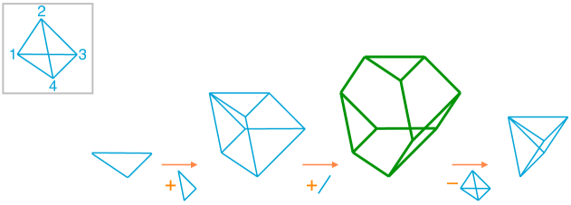
Figure 4: Building up the Minkowski sum $\Delta_{134}+\Delta_{234}+\Delta_{12}=O_{M}$ and the signed Minkowski sum $\Delta_{134}+\Delta_{234}+\Delta_{12}-\Delta_{1234}=P_{M}$ one step at a time.

Theorem 1.8.

If a matroid $M$ on $[n]$ has rank $r$, then the cocircuit polytope $O_{M}$

1. is given by the equation $\sum_{i=1}^{n}x_{i}=D([n])$ and the inequalities $\sum_{i\in S}x_{i}\leq D(S)\textrm{ for }S\subseteq[n]$, where $D(S)$ is the number of cocircuits intersecting $S$,

2. has dimension $n-c$ where $c$ is the number of connected components of $M$,

3. has the matroid polytope $P_{M}=\mathrm{conv}\{e_{B}\,:\,B\textrm{ basis}\}$ as a Minkowski summand,

4. has at most $r!\cdot b$ vertices, where $b$ is the number of bases.

Before we prove this theorem, it is useful to recall some basic facts about generalized permutahedra [Pos09]. The permutahedron $\Pi_{n}$ is the convex hull of the $n!$ permutations of $\{1,\ldots,n\}$ in $\mathbb{R}^{n}$; its normal fan is the braid arrangement formed by the hyperplanes $x_{i}=x_{j}$ for $i\neq j$. A generalized permutahedron is a polytope $P$ obtained from $\Pi_{n}$ by moving the vertices (possibly identifying some of them) while preserving the edge directions. This is equivalent to requiring that the normal fan of $P$ is a coarsening of the braid arrangement. [PRW08]

Every generalized permutahedron is of the form

$$P_{n}(\{z_{I}\})=\{(t_{1},\ldots,t_{n})\in\mathbb{R}^{n}:\sum_{i=1}^{n}t_{i}=z_{[n]},\sum_{i\in I}t_{i}\leq z_{I}\textrm{ for all }I\subseteq[n]\large\}$$

where $z_{I}$ is a minimally chosen real number for each $I\subseteq[n]$, and $z_{\emptyset}=0$. The vector $(z_{I})_{I\subseteq[n]}$ is submodular; that is, $z_{I}+z_{J}\geq z_{I\cup J}+z_{I\cap J}$ for all subsets $I$ and $J$ of $[n]$. Furthermore, this is a bijection between generalized permutahedra and points in the submodular cone in $\mathbb{R}^{2^{n}}$ defined by the submodular inequalities. [AA11, MPS⁺09, Pos09, Sch03]. This shows that generalized permutahedra are essentially the same as polymatroids, which predate them.

There is an alternative description of generalized permutahedra. Every Minkowski sum of simplices of the form $\Delta_{I}$ is a generalized permutahedron [Pos09] and, conversely, every generalized permutahedron can be expressed as a signed sum of such simplices. [ABD10] This automatically implies that $O_{M}$ is a generalized permutahedron. Also, $P_{M}$ is the generalized permutahedron $P_{n}(r(I))_{I\subset[n]}$ where $r(I)$ is the rank of $I$ in the matroid $M$. [ABD10, Sch03]

Proof of Theorem 1.8.

For a polytope $P\in\mathbb{R}^{n}$ and a linear functional $w\in(\mathbb{R}^{n})^{*}$, let $P_{w}$ be the face of $P$ minimized by $w$.

(a) Since $O_{M}$ is a generalized permutahedron, we have $O_{M}=P_{n}({z_{I}})$ for some vector $z_{I}$. Notice that $\Delta_{D}=P_{n}({z^{D}_{I}})$ where $z^{D}_{I}$ is $1$ if $I\cap D\neq\emptyset$ and $0$ otherwise. Then the result follows from the fact that $P_{n}(\{z_{I}\})+P_{n}(\{z^{\prime}_{I}\})=P_{n}(\{z_{I}+z^{\prime}_{I}\})$.

(b) From the Minkowski sum expression for $O_{M}$ it is clear that the edge directions of $O_{M}$ are precisely the edge directions of the various $\Delta_{D}$. These are the vectors of the form $e_{c}-e_{d}$ where $c$ and $d$ are in the same cocircuit; that is, in the same connected component of $M^{*}$. Their span is the subspace given by the equations $\sum_{i\in K_{a}}x_{i}=0$ for the connected components $K_{1},\ldots,K_{c}$ of $M^{*}$, which are also the connected components of $M$. The result follows.

(c) When $M$ is the matroid of a linear ideal $I$, this claim is related to (but not implied by) Proposition 2.3 and the fact that the matroid polytope is a state polytope of $I$. [Stu96, Proposition 2.11] We proceed as follows.

We know that $O_{M}=P_{n}(\{D(I)\})$ and $P_{M}=P_{n}(\{r(I)\})$, where $r$ is the rank function of $M$. We claim that $q(I)=D(I)-r(I)$ is a submodular function; it will then follow that $Q=P_{n}(\{q(I)\})$ is a generalized permutahedron such that $O_{M}=P_{M}+Q$.

Let $\delta_{q}(S,a,b)=-q(S\cup a\cup b)+q(S\cup a)+q(S\cup b)-q(S)$ for $S\subset[n]$ and $a,b\in[n]-S$; define $\delta_{D}$ and $\delta_{r}$ analogously. We will prove that $\delta_{q}$ is always non-negative; this property of “local submodularity” of $q(I)$ implies its submodularity.

Assume contrariwise that $\delta_{q}(S,a,b)<0$. Notice that $\delta_{D}$ and $\delta_{r}$ is non-negative because $D$ and $r$ are submodular, and $\delta_{r}$ equals $0$ or $1$ because $r(S\cup s)-r(S)=0\textrm{ or }1$ for $s\notin S$. Therefore, to have $\delta_{q}(S,a,b)=\delta_{D}(S,a,b)-\delta_{r}(S,a,b)<0$, we must have

$$\delta_{D}(S,a,b)=0,\qquad\delta_{r}(S,a,b)=1.$$ (1)

To have $\delta_{r}(S,a,b)=1$, we must have, for some s,

$$r(S)=s,\qquad r(S\cup a)=r(S\cup b)=r(S\cup a\cup b)=s+1.$$ (2)

One easily checks that $\delta_{D}(S,a,b)=0$ is the number of cocircuits containing $a$ and $b$ and not intersecting $S$. Since hyperplanes are the complements of cocircuits, it follows that every hyperplane $H\supset S$ must contain either $a$ or $b$. If a hyperplane $H\supset S$ contained one and not the other, say $a\in H$ and $b\notin H$, submodularity would imply

$$1=r(H\cup b)-r(H)\leq r(S\cup a\cup b)-r(S\cup a)=0$$

by (2) and the fact that $H$ is a hyperplane. Therefore every hyperplane $H\supset S$ must contain both $a$ and $b$, so every hyperplane of $M/S$ contains both $a$ and $b$. This is only possible if $a$ and $b$ have rank $0$ in $M/S$, which contradicts that $r(S\cup a)=r(S)+1$.

(d) Since the normal fan of $O_{M}$ coarsens the braid arrangement, $\{(O_{M})_{\pi}\,:\,\pi\textrm{ is a permutation of }[n]\}$ is a complete list of the vertices of $O_{M}$, possibly with repetitions. The $\pi$-minimal vertex is

$$(O_{M})_{\pi}=\sum_{D\textrm{ cocircuit of }M}(\Delta_{D})_{\pi}=\sum_{D\textrm{ cocircuit of }M}e_{\min_{\pi}(D)}=(d^{\pi}_{1},\ldots,d^{\pi}_{n})$$

where $d^{\pi}_{i}$ is the number of cocircuits of $M$ whose $\pi$-smallest element is $i$.

Next we observe that the support of any vertex $(O_{M})_{\pi}$ of $O_{M}$ is a basis of $M$; more specifically,

$$\textrm{supp}(O_{M})_{\pi}=B_{\pi}$$ (3)

where $B=B_{\pi}$ denotes the $\pi$-minimal basis of $M$, which minimizes $\sum_{b\in B}\pi(b)$. This basis is unique by the greedy algorithm for matroids. The claim (3) follows from the following variant of the greedy algorithm for matroids due to Tarjan called the blue rule. [Koz91, Theorem 2.7] To construct the $\pi$-minimum basis $B_{\pi}$, we start with all elements of $[n]$ uncolored. We successively choose a cocircuit with no blue elements, and color its smallest element blue. We do this repeatedly, in any order, until it is no longer possible. In the end, the set of blue elements is the basis $B_{\pi}$. Clearly the blue elements are precisely those $i$ such that $d_{i}^{\pi}\neq 0$.

Finally, it remains to observe that for each $\pi$, the vertex $(O_{M})_{\pi}$ is determined uniquely by $M$ and the relative order of $\pi(B_{\pi})$. To see this, notice that $d^{\pi}_{i}$ is the number of cocircuits $D$ of $M$ such that $\pi(i)$ is the smallest element of $\pi(B_{\pi}\cap D)$. This number only depends on the matroid $M$, the basis $B_{\pi}$, and the relative order of $\pi(B_{\pi})$. Since there are $b$ choices for $B_{\pi}$ and $r!$ choices for the relative order of $\pi(B_{\pi})$, the desired result follows. ∎

5 External activity complexes and the primary decomposition.

Let $M$ be a matroid and let $<$ be a linear order on the ground set $E$. We will build a simplicial complex on the $2|E|$-element set $\{x_{e},y_{e}\,:\,e\in E\}$ closely related to the basis activities in $M$. Basis activities were originally defined by Tutte (for graphs) and Crapo (for matroids) to give a combinatorial interpretation of the coefficients of the Tutte polynomial, as described in Theorem 2.6. [Tut54, Cra69] Their clever definition manifests itself algebraically in a very natural way iin our work, thanks to Theorem 1.3(f) and the following result.

We identify subsets and monomials, and write, for $A,B\subseteq E$,

$$x_{A}y_{B}:=\{x_{a}\,:a\in A\}\cup\{y_{b}\,:\,b\in B\}.$$

Theorem 5.1.

Let $M$ be a matroid on $E$ and let $<$ be a linear order on $E$. There is a simplicial complex $B_{<}(M)$ on $\{x_{e},y_{e}\,:\,e\in E\}$, called the external activity complex of $M$ with respect to $<$, such that

1. The facets of $B_{<}(M)$ are the sets $x_{B\cup EP(B)}y_{B\cup EA(B)}$ for each basis $B$, where $EP(B)$ and $EA(B)$ are the sets of externally passive and externally active elements with respect to $B$.

2. The minimal non-faces are $x_{\min C}y_{C-\min C}$ for each circuit $C$.

Proof.

We need to prove that, for $S,T\subseteq E$

$x_{S}y_{T}\subseteq x_{B\cup EP(B)}y_{B\cup EA(B)}$ for some basis $B$

if and only if

$x_{S}y_{T}\not\supseteq x_{\min C}y_{C-\min C}$ for all circuits $C$.

First we prove the forward direction. Assume, contrariwise, that $x_{S}y_{T}\subseteq x_{B\cup EP(B)}y_{B\cup EA(B)}$ for some basis $B$ and $x_{S}y_{T}\supseteq x_{\min C}y_{C-\min C}$ for some circuit $C$. Then

$$x_{\min C}y_{C-\min C}\subseteq x_{B\cup EP(B)}y_{B\cup EA(B)}.$$

Let $\min C=c$. Since $c\in B\cup EP(B)$, there are two cases:

If $c\in B$: Let $D=D(B,c)$ be the fundamental cocircuit. Then $c\in C\cap D$ and, since $|C\cap D|\neq 1$, we can find another element $d\in C\cap D$. Since $d\in D(B,c)$, we have $c\in C(B,d)$; and $c<d$ because $c=\min C$, so $d$ is not externally active in $B$. Also, $d\in D(B,c)$ implies that $d\notin B$. Therefore $d\notin B\cup EA(B)$. This contradicts that $C-\min C\subseteq B\cup EA(B)$.

If $c\in EP(B)$: We have $c\notin B$. We can find an element $d\in C(B,c)$ with $d<c$. Now $d\in C(B,c)$ implies $c\in D(B,d)=:D$, so $c\in C\cap D$. Again, this means we can find another $e\in C\cap D$. Since $e\in C$ and $c=\min C$, we have $c<e$, and therefore $d<e$. Now, $e\in D$ implies that $e\notin B$. Also $e\in D(B,d)$ implies that $d\in C(B,e)$; and $d<e$ then implies that $e\notin EA(B)$. Therefore $e\notin B\cup EA(B)$. Again, this contradicts that $C-\min C\subseteq B\cup EA(B)$. This completes the proof of the forward direction.

To prove the backward direction, assume that $x_{S}y_{T}\not\subseteq x_{B\cup EP(B)}y_{B\cup EA(B)}$ for all bases $B$. We need to show that $x_{S}y_{T}\supseteq x_{\min C}y_{C-\min C}$ for some circuit $C$.

By Theorem 2.6 we can write $T=B\cup E-I$ for some basis $B$, some subset $E\subseteq EA(B)$, and some subset $I\subseteq IA(B)$. Then $T\subseteq B\cup EA(B)$, so $S\not\subseteq B\cup EP(B)$. Therefore we can find $s\in S$ with $s\notin B\cup EP(B)$; that is, $s\in EA(B)$.

Let $C=C(B,s)$. We claim that $x_{S}y_{T}\supseteq x_{\min C}y_{C-\min C}$. Since $s\in EA(B)$, $s=\min C$, so $S\supseteq\min C$. It remains to show that $T\supseteq C-\min C$. Assume, contrariwise, that $d\in C-\min C$ but $d\notin T$. Since $d\in C-\min C$, $d\in B$. Since $d\notin T=B\cup E-I$, this implies that $d\in I$, so $d$ is internally active in $B$. Therefore $d$ is the smallest element in $D(B,d)$. But $d\in C(B,s)$ implies that $s\in D(B,d)$, which implies that $s>d$. This contradicts that $s=\min C$. The desired result follows. ∎

Theorem 5.2.

Let $M$ be a matroid on $E$ and let $<$ be a linear order on $E$. The ideal

$$C(M,<)=\left<x_{c_{1}}y_{c_{2}}y_{c_{3}}\cdots y_{c_{k}}\,:\,C=\{c_{1},\ldots,c_{k}\}\textrm{ is a circuit of $M$ and $c_{1}=\min_{<}C$}\right>$$

in ${\mathbbm{k}}[x_{e},y_{e}\,:\,e\in E]$ is the Stanley-Reisner ideal of the external activity complex $B_{<}(M)$. Its primary decomposition is

$$C(M,<)=\bigcap_{B\textrm{ basis of }M}\left<\,x_{e}\,:\,e\in EA_{<}(B)\,,\,y_{e}\,:\,e\in EP_{<}(B)\right>.$$

Proof.

By Theorem 5.1.1, $C(M,<)$ is the Stanley-Reisner ideal of $B_{<}(M)$. Theorem 5.1.2 and [MS05, Theorem 1.7] then imply the desired primary decomposition. ∎

The external activity complex and the corresponding monomial ideal are closely related to two important simplicial complexes from matroid theory. If we set $y_{i}=x_{i}$ we obtain the Stanley-Reisner ideal of the independence complex of $M$, whose facets are the bases of $M$. If we set $x_{i}=1$ we get the Stanley-Reisner ideal of the broken circuit complex of $M$, whose facets are the nbc-bases of $M$. [Bjö92]

6 Proofs of our main theorems.

Having built up the necessary combinatorial background, we now use algebraic and geometric tools to complete the proof of our main theorems.

Theorem 1.3.

Let $L\subset\mathbb{A}^{n}$ be a $d$-dimensional linear space and let ${\widetilde{L}}\subset(\mathbb{P}^{1})^{n}$ be the closure of $L$ induced by the embedding $\mathbb{A}^{n}\subset(\mathbb{P}^{1})^{n}$. Let $M$ be the matroid of $L$; it has rank $r=n-d$. Then:

1. The homogenized cocircuits of $I(L)$ minimally generate the ideal $I(\widetilde{L})$.

2. The homogenized cocircuits of $I(L)$ form a universal Gröbner basis for $I(\widetilde{L})$, which is reduced under any term order.

3. The $\mathbb{Z}^{n}$-multi-degree of $\widetilde{L}$ is $\sum\limits_{B}t_{b_{1}}\cdots t_{b_{r}}$ summing over all bases $B=\{b_{1},\ldots,b_{r}\}$ of $M$.

4. The bidegree of $\widetilde{L}$ is $t^{r}h_{M}(s/t)$ where $h_{M}$ is the $h$-polynomial of $M$.

5. There are at most $r!\cdot b$ distinct initial ideals of $I(\widetilde{L})$, where $b$ is the number of bases of $M$.

6. The initial ideal $\operatorname{in}_{<}I(\widetilde{L})$ is the Stanley–Reisner ideal of the external activity complex $B_{<}(M^{*})$ of the dual matroid $M^{*}$. Its primary decomposition is:

   $$\operatorname{in}_{<}I(\widetilde{L})=\bigcap_{B\textrm{ basis }}\left<\,x_{e}\,:\,e\in IA_{<}(B)\,,\,y_{e}\,:\,e\in IP_{<}(B)\right>$$

   where $B=IA_{<}(B)\,\sqcup\,IP_{<}(B)$ is the partition of $B$ into internally active and passive elements with respect to $<$.

One of our goals is to show that the set $G=\{f_{C}^{h}\}$ of homogenized circuits is a universal Gröbner basis (UGB); that is, a Gröbner basis for $I(\widetilde{L})$ with respect to any term order. One key tool is the following: If two ideals share the same codimension and degree and one contains the other, then under suitably nice conditions we can say they are equal.

Proof of (c).

We compute the multi-degree of $\widetilde{L}$ using a geometric argument, recalling the discussion of Section 3.2. For each $\Delta=\{i_{1},\ldots,i_{r}\}\subset[n]$ we let $Z_{\Delta}=\prod_{i\in\Delta}(\mathbb{P}^{1})_{i}\times\prod_{i\notin\Delta}q_{i}$, where $q_{i}$ is a generic point in $(\mathbb{P}^{1})_{i}$ for each $i\notin\Delta$. Then we have

$$\textrm{mdeg }\widetilde{L}=\sum_{\Delta\in{[n]\choose r}}m(Z_{\Delta},\widetilde{L})t_{i_{1}}\cdots t_{i_{r}}.$$

where $m(Z_{\Delta},\widetilde{L})$ is the number of points in $Z_{\Delta}\cap\widetilde{L}$ counted with multiplicity. We will prove that

$$m(Z_{\Delta},\widetilde{L})=\begin{cases}1&\text{if }\Delta\text{ is a basis of $M$, and}\\ 0&\textrm{otherwise,}\end{cases}$$

from which our formula for $\textrm{mdeg }{\widetilde{L}}$ will follow.

First let $\Delta$ be a basis., Since the points $q_{i}$ in $Z_{\Delta}$ are general, we may suppose that $y_{i}\neq 0$ for $i\notin\Delta$. Now let $i\in\Delta$. Since $\Delta$ is a basis, there is a cocircuit $D$ containing $i$ whose support is contained in $([n]-\Delta)\cup i$; in fact, this is the fundamental cocircuit $D(\Delta,i)$. If $y_{i}$ were equal to zero, then the homogenized cocircuit equation $f_{D}^{h}=0$ would force $x_{i}=0$, which is impossible. Hence all intersections must occur in the affine patch where no coordinate $y_{i}$ equals zero; but then we are working in the original affine space, so it is clear that $Z_{\Delta}\cap\widetilde{L}=Z_{\Delta}\cap L$ is a single point with no multiplicity. Therefore $m(Z_{\Delta},\widetilde{L})=1$.

On the other hand, if $\Delta=\{i_{1},\ldots,i_{r}\}$ is not a basis, then there is a cocircuit $D$ which is disjoint from $\Delta$. This means that $Z_{\Delta}$ does not meet the hypersurface defined by the homogenized cocircuit $f_{D}^{h}$. Hence $\widetilde{L}$ does not meet $Z_{\Delta}$ and $m(Z_{\Delta},\widetilde{L})=0$. The desired result follows. ∎

Proof of (b).

Let $G=\{f_{D}^{h}\,:\,D\textrm{ cocircuit of }M\}\subset I(\widetilde{L})$ denote the set of homogenized cocircuits. Let $<$ be any monomial term order on ${\mathbbm{k}}[x_{1},\ldots,x_{n},y_{1},\ldots,y_{n}]$, and let $\operatorname{in}_{<}G$ denote the ideal generated by the leading terms of the polynomials in $G$. We need to show that $\operatorname{in}_{<}G=\operatorname{in}_{<}I(\widetilde{L})$. We begin with a remark:

Remark 6.1.

If $<$ is any monomial term order, it is sufficient for Gröbner computations to assume that $<$ is given by a weight order $w$ on the $2n$ variables $x_{1},\ldots,x_{n},y_{1},\ldots,y_{n}$. [Stu96, Prop. 1.11] Since all of the polynomials in $I(\widetilde{L})$ are multi-homogeneous, the term order $w^{\prime}$ given by

$$\begin{array}[]{rcl}w^{\prime}(x_{i})&=&w(x_{i})-w(y_{i})\\ w^{\prime}(y_{i})&=&0\end{array}$$

will pick out the same initial terms on $I(\widetilde{L})$ as $w$. Thus we may assume that the weights on the $y$ variables are all zero. The resulting linear order on $1,\ldots,n$ is the reverse of the linear order that we imposed on $[n]$ in Remark 7.4.

Notice that each term of a given $f_{D}^{h}$ has degree one in the $y$-variables and is homogeneous. Thus by the remark, the leading term of $f_{D}^{h}$ depends only on the linear order on $1,\ldots,n$. Therefore

$$\operatorname{in}_{<}G=\left<x_{d_{1}}y_{d_{2}}y_{d_{3}}\cdots y_{d_{k}}\,:\,D=\{d_{1},\ldots,d_{k}\}\textrm{ is a cocircuit of $M$ and $d_{1}=\min_{<}D$}\right>.$$

In other words,

$$\operatorname{in}_{<}G=C(M^{*},<)$$

is the Stanley-Reisner ideal of the external activity complex $B_{<}(M^{*})$ of $M^{*}$, as described in Theorem 5.2. Therefore

$$\operatorname{in}_{<}G=\bigcap_{B\textrm{ basis of }M}\left<\,x_{e}\,:\,e\in IA_{<}(B)\,,\,y_{e}\,:\,e\in IP_{<}(B)\right>.$$ (4)

Applying Proposition 3.3 to (4) then gives

$$\textrm{mdeg }\operatorname{in}_{<}G=\sum\limits_{B\textrm{ basis}}t_{b_{1}}\cdots t_{b_{r}}=\textrm{mdeg }I(\widetilde{L}).$$

We also have that

$$\textrm{mdeg }I(\widetilde{L})=\textrm{mdeg }\operatorname{in}_{<}I(\widetilde{L}).$$

since multi-degree is preserved by flat degenerations. Therefore both ideals in the inclusion

$$\operatorname{in}_{<}G\subset\operatorname{in}_{<}I(\widetilde{L})$$

have the same multidegree. Since the smaller ideal is reduced and equidimensional, this implies that $\operatorname{in}_{<}G=\operatorname{in}_{<}I(\widetilde{L})$. [KM05, Lemma 1.7.5]. Since $<$ was arbitrary, $G=\{f_{C}^{h}\}$ is a universal Gröbner basis for $I(\widetilde{L})$. To see that $G$ is reduced for each term order, just notice that no term divides another, because no cocircuit contains another. ∎

Proof of (f).

Now that we know that $\operatorname{in}_{<}G=\operatorname{in}_{<}I(\widetilde{L})$, this follows from (4). ∎

Proof of (d).

By (f) and Theorem 2.6, any initial ideal has bidegree $t^{r}h_{M}(s,t)$. The result then follows from the fact that bidegree is degenerative. [MS05] ∎

Proof of (a).

Since no term of any generator in $G$ divides any other term, the elements of $G$ are linearly independent over ${\mathbbm{k}}$, and they minimally generate $\left<G\right>=I(\widetilde{L})$. ∎

Proof of (e).

Finally we prove our upper bound for the number of distinct initial ideals of $\operatorname{in}_{<}I(\widetilde{L})$. One way to proceed is to invoke [Stu96, Cor. 2.9]: if $G$ is a universal Gröbner bases of $I$ which is a reduced Gröbner bases with respect to any term order $<$, then the Minkowski sum $\sum_{g\in G}\textrm{New}(g)$ is a state polytope for $I$, so its vertices are in bijection with the initial ideals of $I$. Here $\textrm{New}(g)$ denotes the Newton polytope of $g$. The Newton polytope of each homogenized cocircuit $f_{D}^{h}$ is, after translation, equal to $\nabla_{I}=\mathrm{conv}\{h_{i}\,:\,i\in I\}$, where $h_{d}=f_{d}-g_{d}$ and $f_{1},\ldots,f_{n},g_{1},\ldots,g_{n}$ is the standard basis for $\mathbb{R}^{2n}$. It follows that $\sum_{f_{D}^{h}\in G}\textrm{New}(g)=\sum_{D\textrm{ cocircuit}}\nabla_{D}$ is affinely isomorphic to $\sum_{D\textrm{ cocircuit}}\Delta_{D}=O_{M}$. The result then follows by Theorem 1.8(d).

We also give a self-contained algebraic proof. If we take an initial ideal of $I(\widetilde{L})$ and set all the $y$-variables equal to $1$, then we obtain an initial ideal of $I(L)$. Hence we have a map

$$\{\textrm{initial ideals of }I(\widetilde{L})\}\stackrel{{\scriptstyle\rho}}{{\to}}\{\textrm{initial ideals of }I(L)\}.$$

This map is surjective since the cocircuits and their homogenizations are universal Gröbner bases.

Each initial ideal $\operatorname{in}_{<}I(\widetilde{L})$ of $I(L)$ is of the form $I_{B}=\langle x_{b_{1}},\ldots,x_{b_{r}}\rangle$, where $B=\{b_{1},\ldots,b_{r}\}$ is the $<$-minimum basis of $B$. [Stu96, Prop. 2.11] Hence the map $\rho$ is surjective onto a set with $b$ elements. The pre-image of $I_{B}$ is a set of ideals in the $x$ and $y$ variables. Now, any term order which determines an ideal in $\rho^{-1}(I_{B})$ obviously always selects a term from each homogenized cocircuit with an $x_{b_{i}}$ for some $i$. Hence, the relative order of the variables $x_{b_{i}}$ is sufficient to determine $\operatorname{in}_{<}I(\widetilde{L})$. There are $r!$ such orders, so the number of initial ideals of $I(\widetilde{L})$ is at most $r!\cdot b$. ∎

Theorem 1.5.

Let $L$ be a linear $d$-space in $\mathbb{A}^{n}$, and $I(\widetilde{L})$ the ideal of its closure in $(\mathbb{P}^{1})^{n}$. The non-zero multigraded Betti numbers of $S/I(\widetilde{L})$ are precisely:

$$\beta_{i,{\textbf{a}}}(S/I(\widetilde{L}))=|\mu(F,\widehat{1})|$$

for each flat $F$ of $M$, where $i=r-r(F)$, and ${\textbf{a}}=e_{[n]-F}$. Here $\mu$ is the Möbius function of the lattice of flats of $M$. Furthermore, all of the initial ideals have the same Betti numbers:

$$\beta_{i,{\textbf{a}}}(S/I(\widetilde{L}))=\beta_{i,{\textbf{a}}}(S/(\operatorname{in}_{<}I(\widetilde{L})))$$

for all a and for every term order $<$.

Proof.

As we already remarked, the initial ideal

$$\operatorname{in}_{<}I({\widetilde{L}})=C(M^{*},<)=\left<x_{d_{1}}y_{d_{2}}y_{d_{3}}\cdots y_{d_{k}}\,:\,D=\{d_{1},\ldots,d_{k}\}\textrm{ is a cocircuit of $M$ and $d_{1}=\min_{<}D$}\right>$$

is closely related to the Stanley-Reisner ideal

$$I_{IN(M^{*})}=\left<x_{d_{1}}x_{d_{2}}\cdots x_{d_{k}}\,:\,D=\{d_{1},\ldots,d_{k}\}\textrm{ is a cocircuit of $M$}\right>$$

of the independence complex $IN(M^{*})$ of the dual matroid $M^{*}$. More precisely, the second is obtained from the first by setting $y_{i}=x_{i}$. In fact, we now show that this substitution is equivalent to taking $C(M^{*},<)$ modulo a regular sequence. This will follow from the primary decomposition of $\operatorname{in}_{<}I({\widetilde{L}})$ given by Theorem 5.2, together with the following lemma:

Lemma 6.2.

Let $I$ be a squarefree monomial ideal in $S={\mathbbm{k}}[x_{1},\ldots,x_{n},y_{1},\ldots,y_{n}]$ satisfying

• For each $i$, no associated prime of $I$ contains both $x_{i}$ and $y_{i}$, and

• No minimal generator of $I$ contains a product of the form $x_{i}y_{i}$.

Then

$$\{x_{1}-y_{1},\ldots,x_{n}-y_{n}\}$$

is a regular sequence on $S/I$.

Proof.

Notice that (P1) implies that $x_{1}-y_{1}$ is a regular element on $S/I$. We now form the ideal

$$I^{\prime}=I\otimes S/(x_{1}-y_{1})$$

which we realize as an ideal in the polynomial ring $S/(x_{1})$ via the substitution $x_{1}\mapsto y_{1}$. We claim that $I^{\prime}$ has properties $(P1),(P2)$ and then the proof will be complete by induction.

First, the minimal generators of $I^{\prime}$ are precisely the generators of $I$ after the substitution $x_{1}\mapsto y_{1}$. Thus (P2) is satisfied.

Now denote the primary decomposition of $I$ as $I=\bigcap P_{i}.$ Let $P^{\prime}_{i}$ denote the ideal obtained from $P_{i}$ after the substitution $x_{1}\mapsto y_{1}$. We claim that

$$I^{\prime}=\bigcap P^{\prime}_{i}.$$

Substitution is a ring map, and this easily implies the inclusion $I^{\prime}\subset\bigcap P^{\prime}_{i}$. For the opposite conclusion, suppose that $f$ is a minimal generator of $\bigcap P^{\prime}_{i}$. We need to show that $f\in I^{\prime}$. Notice that $f$ does not involve $x_{1}$. We have two cases:

Case 1: $y_{1}$ does not divide $f$. In this case, $f\in P^{\prime}_{i}$ implies $f\in P_{i}$ for all $i$, so $f\in I$. But then $f\in I^{\prime}$ also, since $f$ does not involve $x_{1}$ or $y_{1}$, the variables that change under our substitution.

Case 2: $y_{1}$ divides $f$, say $f=y_{1}g$. Consider the element $h=x_{1}f$. Since $h$ is divisible by both $x_{1}$ and $y_{1}$, and since $f$ is in $\bigcap P^{\prime}_{i}$, we know $h$ is in fact in each ideal $P_{i}$. Thus $h=x_{1}y_{1}g\in I$. But since $I$ has no minimal generators by (P1) divisible by $x_{1}y_{1}$ we know that either $x_{1}g$ or $y_{1}g$ must be in $I$. Under the substitution, both of these elements will be sent to $f$, so that $f\in I^{\prime}$.

We conclude that indeed $I^{\prime}=\bigcap P^{\prime}_{i}$, which implies that $I^{\prime}$ satisfies (P1). This completes the proof by induction. ∎

With Lemma 6.2 at hand, we are now ready to prove Theorem 1.5. As taking initial ideals is a flat degeneration, we have

$$\beta_{i,{\textbf{a}}}(S/I(\widetilde{L}))\leq\beta_{i,{\textbf{a}}}(S/(\operatorname{in}_{<}I(\widetilde{L}))).$$

for all $i$ and a. As explained in Section 3.1, the only way that this inequality can be strict is due to a consecutive cancellation in the minimal free resolution of $S/\operatorname{in}_{<}I(\widetilde{L})$. This requires that $\beta_{i,{\textbf{a}}}(S/(\operatorname{in}_{<}I(\widetilde{L})))$ is nonzero for some a and for two consecutive values of $i$. However, since $\{x_{1}-y_{1},\ldots,x_{n}-y_{n}\}$ is a regular sequence by the previous Lemma, we know that the Betti numbers of $S/(\operatorname{in}_{<}I(\widetilde{L}))$ equal those of the independence ideal ${\mathbbm{k}}[x_{1},\ldots,x_{n}]/I_{IN(M^{*})}$. Theorem 2.9 then shows that no such consecutive cancellations are possible. ∎

Theorem 1.6.

If $L$ is a linear space the ideal $I(\widetilde{L})$ and all of its initial ideals are Cohen-Macaulay.

Proof.

An ideal is Cohen-Macaulay if an only if its codimension is equal to its projective dimension. Since both ideals are of the same codimension and

$$\beta_{i,{\textbf{a}}}(S/I(\widetilde{L}))=\beta_{i,{\textbf{a}}}(S/(\operatorname{in}_{<}I(\widetilde{L})))$$

by Theorem 1.5, it is sufficient to prove that $\operatorname{in}_{<}I(\widetilde{L})$ is Cohen-Macaulay.

Now, Theorem 1.5 also tells us that the projective dimension of $S/(\operatorname{in}_{<}I(\widetilde{L}))$ equals $r$, the rank of $M$. Also since $S/(\operatorname{in}_{<}I(\widetilde{L}))$ is the Stanley-Reisner ring of $B_{<}(M^{*})$, whose facets have $2n-r$ elements, its codimension is also $r$. The desired result follows. ∎

7 The non-homogeneous case: affine linear spaces.

So far, we have assumed that the linear space $L$ was actually a vector subspace of ${\mathbbm{k}}^{n}$. This is a minor assumption, but nonetheless, the nonhomogeneous case has some interesting features.

In this section, suppose that $L$ is an affine linear subspace defined by the matrix equation

$$A\cdot\vec{x}=\vec{b},$$

and let $\widetilde{L}$ be its closure in $(\mathbb{P}^{1})^{n}$. Now the invariants of $\widetilde{L}$ are controlled by (any two of) the following triple of matroids $(M_{hom},M,M^{\prime})$:

$\bullet$ the matroid $M$ on $[n]$ that we associated to the subspace $A\cdot\vec{x}=\vec{0}$,

$\bullet$ the augmented matroid $M_{hom}$ on $[0,n]$ associated to the subspace $(A\,|\,(-b))\cdot\overrightarrow{(x,x_{0})}=\vec{0}$,

$\bullet$ the matroid $M^{\prime}$ on $[n]$ of the subspace obtained from $(A\,|\,(-b))\cdot\overrightarrow{(x,x_{0})}=\vec{0}$ by eliminating $x_{0}$.

Any two of these matroids determine the third. They are related by

$$M=M_{hom}\backslash 0,\qquad M^{\prime}=M_{hom}/0.$$

The triple $(M_{hom},M,M^{\prime})$ is equivalent to a pointed matroid [Bry71] or a semimatroid [Ard07].

7.1 Matroid preliminaries: morphisms and Tutte polynomials.

The matroids $M$ and $M^{\prime}$ above can be thought to have the same ground set. They constitute a morphism of matroids, denoted $M\rightarrow M^{\prime}$; this means that every flat of $M^{\prime}$ is a flat of $M$. Just as matroids are an abstraction of vector configurations, matroid morphisms are an abstraction of linear maps.

LasVergnas [LV80] defined the Tutte polynomial of a morphism $M\rightarrow M^{\prime}$ to be

$$T_{M\rightarrow M^{\prime}}(x,y,z)=\sum_{S\subseteq E}(x-1)^{r^{\prime}-r^{\prime}(S)}(y-1)^{|S|-r(S)}z^{rcd_{M,M^{\prime}}(S)}$$

where $r$ and $r^{\prime}$ are the rank functions of $M$ and $M^{\prime}$, and $rcd_{M,M^{\prime}}(S)=(r-r^{\prime})-(r(S)-r^{\prime}(S))$.

He also gave an activity interpretation of this polynomial, which we now describe. For an independent set $X$ of $M$ and $i\notin X$, the set $X\cup i$ contains at most one circuit $C$ of $M$ (which must contain $i$). If $C$ does exist and $i$ is the smallest element in $C$, then we say $i$ is externally active with respect to $X$ in $M$. Dually, for a spanning set $X$ of $M^{\prime}$, the set $(E-X)\cup i$ contains at most one cocircuit $D$ of $M^{\prime}$ (which must contain $i$). If $D$ does exist, and $i$ is the smallest element in $D$, then we say $i$ is internally active with respect to $X$ in $M^{\prime}$.

Theorem 7.1.

[LV80] Consider any matroid morphism $M\rightarrow M^{\prime}$ and any linear order $<$ on the ground set $E$ of $M$ and $M^{\prime}$. Then

$$T_{M\rightarrow M^{\prime}}(x,y,z)=\sum_{S\subseteq E}x^{|IA^{\prime}(S)|}y^{|EA(S)|}z^{rcd_{M,M^{\prime}}(S)}$$

summing over the sets $S$ which are spanning in $M^{\prime}$ and independent in $M$, where $IA^{\prime}(S)$ represents the set of internally active elements of $S$ in $M^{\prime}$, and $EA(S)$ represents the externally active elements with respect to $S$ in $M$.

7.2 A non-homogeneous example.

Before we state and prove our theorems about affine subspaces, we carry out an example in detail which displays most of the interesting features.

Example 7.2.

Consider the affine subspace $L$ of $\mathbb{A}^{6}$ given by the linear ideal

$$I(L)=\left<x_{1}+x_{2}+x_{6}+a,\,\,x_{2}-x_{3}+x_{5}+b,\,\,x_{3}+x_{4}+c\right>,$$

where $a,b,c$ are parameters.

The matroid $M$ is the same one of Example 1.7, while $M_{hom}$ is the matroid of the ideal

$$I(L_{hom})=\left<x_{1}+x_{2}+x_{6}+ax_{0},\,\,x_{2}-x_{3}+x_{5}+bx_{0},\,\,x_{3}+x_{4}+cx_{0}\right>.$$

in seven variables, defining a linear space $L_{hom}$ in $\mathbb{A}^{7}$. We can also see $M_{hom}$ as the matroid obtained by adding the point $(a,b,c)$ to our point configuration of columns.

From now on we assume $(a,b,c)=(1,0,1)$. Figure 5 shows the enlarged point configuration, the original point configuration, and the contracted point configuration. They correspond, respectively, to the matroids $M_{hom}$, $M$, and $M^{\prime}$.

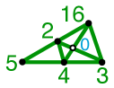
Figure 5: The triple $(M_{hom},M,M^{\prime})$ corresponding to the affine subspace $L$.

Notice that every basis of $M$ is still a basis in $M_{hom}$. Every cocircuit of $M$ gives rise to a cocircuit of $M_{hom}$ by adding $0$ if necessary. As a partial converse, every cocircuit of $M_{hom}$ contains a cocircuit of $M$. Furthermore, if $D$ is a cocircuit of $M_{hom}$ containing $0$, then $D-0$ is a cocircuit of $M$. In our example the cocircuits are:

$${\cal D} = \{126,\,\,1356,\,\,1456,\,\,235,\,\,245,\,\,34\}$$

$${\cal D}_{hom} = \{0126,01356,1456,235,0245,034,12346\}$$

We will show in Theorem 7.3 that the six homogenized cocircuits of $I(L)$, which correspond to the cocircuits ${\cal D}$ of $M$, minimally generate $I(\widetilde{L})$ and give a universal Gröbner basis:

$$I(\widetilde{L})=\left<{\color[rgb]{0,0,1}x_{1}}y_{2}y_{6}+y_{1}{\color[rgb]{0,0,1}x_{2}}y_{6}+y_{1}y_{2}{\color[rgb]{0,0,1}x_{6}}+1y_{1}y_{2}y_{6},\,\,\ldots,\,{\color[rgb]{0,0,1}x_{3}}y_{4}+y_{3}{\color[rgb]{0,0,1}x_{4}}+1y_{3}y_{4}\right>.$$

Some of the invariants of $I(\widetilde{L})$ depend only on $M$ as before. The multidegree of $\widetilde{L}$ is still given by the thirteen bases of the matroid $M$. The multigraded Betti numbers also stay the same as before.

On the other hand, the initial ideals of $I(\widetilde{L})$ depend on the augmented matroid $M_{hom}$ as well. For $w({\color[rgb]{0,0,1}x_{1}}/y_{1})>\cdots>w({\color[rgb]{0,0,1}x_{6}}/y_{6})>0$, the initial ideal $\operatorname{in}_{<}I(\widetilde{L})$ is the same as in the homogeneous case:

$$\operatorname{in}_{<}I(\widetilde{L}) = \left<{\color[rgb]{0,0,1}x_{1}}y_{2}y_{6},\,\,{\color[rgb]{0,0,1}x_{1}}y_{3}y_{5}y_{6},\,\,{\color[rgb]{0,0,1}x_{1}}y_{4}y_{5}y_{6},\,\,{\color[rgb]{0,0,1}x_{2}}y_{3}y_{5},\,\,{\color[rgb]{0,0,1}x_{2}}y_{4}y_{5},\,\,{\color[rgb]{0,0,1}x_{3}}y_{4}\right>$$

$$= \left<{\color[rgb]{0,0,1}x_{1}},{\color[rgb]{0,0,1}x_{2}},{\color[rgb]{0,0,1}x_{3}}\right>\,\cap\,\left<{\color[rgb]{0,0,1}x_{1}},{\color[rgb]{0,0,1}x_{2}},y_{4}\right>\,\cap\,\left<{\color[rgb]{0,0,1}x_{1}},y_{3},y_{4}\right>\,\cap\,\left<{\color[rgb]{0,0,1}x_{1}},{\color[rgb]{0,0,1}x_{3}},y_{5}\right>\,\cap\,\left<{\color[rgb]{0,0,1}x_{1}},y_{4},y_{5}\right>\,\cap\,$$

$$\left<y_{2},y_{3},y_{4}\right>\,\cap\,\left<y_{2},{\color[rgb]{0,0,1}x_{3}},y_{5}\right>\,\cap\,\left<x_{2},{\color[rgb]{0,0,1}x_{3}},y_{6}\right>\,\cap\,\left<y_{2},y_{4},y_{5}\right>\,\cap\,\left<{\color[rgb]{0,0,1}x_{2}},y_{4},y_{6}\right>\,\cap\,$$

$$\left<y_{3},y_{4},y_{6}\right>\,\cap\,\left<{\color[rgb]{0,0,1}x_{3}},y_{5},y_{6}\right>\,\cap\,\left<y_{4},y_{5},y_{6}\right>.$$

However, if $0>w({\color[rgb]{0,0,1}x_{1}}/y_{1})>\cdots>w({\color[rgb]{0,0,1}x_{6}}/y_{6})$, we have

$$\operatorname{in}_{<}I(\widetilde{L}) = \left<y_{1}y_{2}y_{6},\,\,y_{1}y_{3}y_{5}y_{6},\,\,{\color[rgb]{0,0,1}x_{1}}y_{4}y_{5}y_{6},\,\,{\color[rgb]{0,0,1}x_{2}}y_{3}y_{5},\,\,y_{2}y_{4}y_{5},\,\,y_{3}y_{4}\right>$$

$$= \left<{\color[rgb]{0,0,1}x_{1}},y_{2},y_{3}\right>\,\cap\,\left<y_{1},{\color[rgb]{0,0,1}x_{2}},y_{4}\right>\,\cap\,\left<y_{1},y_{3},y_{4}\right>\,\cap\,\left<y_{1},y_{3},y_{5}\right>\,\cap\,\left<y_{1},y_{4},y_{5}\right>\,\cap\,$$

$$\left<y_{2},y_{3},y_{4}\right>\,\cap\,\left<y_{2},y_{3},y_{5}\right>\,\cap\,\left<y_{2},y_{3},y_{6}\right>\,\cap\,\left<y_{2},y_{4},y_{5}\right>\,\cap\,\left<{\color[rgb]{0,0,1}x_{2}},y_{4},y_{6}\right>\,\cap\,$$

$$\left<y_{3},y_{4},y_{6}\right>\,\cap\,\left<y_{3},y_{5},y_{6}\right>\,\cap\,\left<y_{4},y_{5},y_{6}\right>.$$

We will see that the 13 primary components still correspond to the 13 bases of $M$. However, in the primary component $\left<z_{i}\,:\,i\in B\right>$, we have $z_{i}={\color[rgb]{0,0,1}x_{i}}$ if $i$ is internally active in $B$ as a basis of $M_{hom}$, and $z_{i}=y_{i}$ otherwise.

Notice that, in contrast with the linear case, $I(\widetilde{L})$ is no longer bihomogeneous under the bigrading $\mathrm{bideg\,\,}{\color[rgb]{0,0,1}x_{i}}=(1,0)$ and $\mathrm{bideg\,\,}y_{i}=(0,1)$. However, some initial ideals still have interesting bidegrees. For any term order with $w({\color[rgb]{0,0,1}x_{1}}/y_{1}),\cdots,w({\color[rgb]{0,0,1}x_{6}}/y_{6})>0$, we saw in Example 1.7 that the bidegree of $\operatorname{in}_{<}I(\widetilde{L})$ is $s^{3}+3s^{2}t+5st^{2}+4t^{3}$. This is essentially the $h$-polynomial of $M$. We will also show that for any term order with $0>w({\color[rgb]{0,0,1}x_{1}}/y_{1}),\cdots,w({\color[rgb]{0,0,1}x_{6}}/y_{6})$, the bidegree of $\operatorname{in}_{<}I(\widetilde{L})$ is $3st^{2}+10t^{3}$. It is not obvious that all these initial ideals should have the same bidegree; this will follow from the fact that this polynomial is an evaluation of the Tutte polynomial of the matroid morphism $M\rightarrow M^{\prime}$.

The number of initial ideals also depends on $M_{hom}$. Table 1 shows these numbers for five choices of $(a,b,c)$. In Figure 1 they correspond, respectively, to adding point $0$ as a loop, as the intersection of lines $23$ and $146$, as a generic point on line $24$, as a generic point on line $136$, or as a generic point in the plane. Somewhat surprisingly, a special choice of $(a,b,c)$ can lead to more initial ideals for $I(\widetilde{L})$ than a generic choice.

$(a,b,c)$	number of initial	number of initial
	ideals of $I(\widetilde{L})$	ideals of $I(\widetilde{L}_{hom})$
$(0,0,0)$	72	72
$(1,0,1)$	124	144
$(2,2,3)$	114	156
$(1,-1,1)$	111	150
$(1,2,3)$	107	162

Table 1: Number of initial ideals for various choices of $(a,b,c)$

For homogeneous linear spaces $L$, we proved that the number of initial ideals of $I(\widetilde{L})$ is at most $r!\cdot b$ where $r=n-d$ is the codimension of $L$ and $b$ is the number of bases of $M(L)$. This bound is visibly false in the non-homogeneous case, as shown in Table 1. Instead, we will prove a bound of $r!\cdot b_{hom}$, where $b_{hom}$ is the number of bases of $M_{hom}$.

The following theorem is the affine analog of Theorem 1.3.

Theorem 7.3.

Let $L\subset\mathbb{A}^{n}$ be a $d$-dimensional affine space and let ${\widetilde{L}}\subset(\mathbb{P}^{1})^{n}$ be the closure of $L$ induced by the embedding $\mathbb{A}^{n}\hookrightarrow(\mathbb{P}^{1})^{n}$. Let $(M_{hom},M,M^{\prime})$ be the triple of matroids of $L$. Then:

1. The homogenized cocircuits of $I(L)$ minimally generate the ideal $I(\widetilde{L})$.

2. The homogenized cocircuits of $I(L)$ form a universal Gröbner basis for $I(\widetilde{L})$, which is reduced under any term order.

3. The $\mathbb{Z}^{n}$-multi-degree of $\widetilde{L}$ is $\sum\limits_{B}t_{b_{1}}\cdots t_{b_{r}}$ summing over all bases $B=\{b_{1},\ldots,b_{r}\}$ of $M$.

4. The bidegree of the ideal $I(\widetilde{L})$ is not well-defined unless $L$ is a linear subspace. However:

   1. For every term order $<$ with $x_{i}>y_{i}$ for all $i$,

   $$\mathrm{bideg\,\,}\operatorname{in}_{<}I(\widetilde{L})=t^{r}h_{M}(s/t),$$

   where $h_{M}(x)=T_{M}(x,1)$ is the $h$-polynomial of $M$ and $T_{M}(x,y)$ is its Tutte polynomial.

   2. For every term order $<$ with $x_{i}<y_{i}$ for all $i$,

   $$\mathrm{bideg\,\,}\operatorname{in}_{<}I(\widetilde{L})=t^{r}T_{M\rightarrow M^{\prime}}(s/t,1,0),$$

   where $T_{M\rightarrow M^{\prime}}(x,y,z)$ is the Tutte polynomial of the matroid morphism $M\rightarrow M^{\prime}$.

5. There are at most $r!\cdot b_{hom}$ distinct initial ideals of $I(\widetilde{L})$, where $b_{hom}$ is the number of bases of $M_{hom}$.

6. The primary decomposition of an initial ideal $\operatorname{in}_{<}I(\widetilde{L})$ is given by:

   $$\operatorname{in}_{<}I(\widetilde{L})=\bigcap_{B\textrm{ basis of }M}\left<\,x_{e}\,:\,e\in IA^{hom}_{<}(B)\,,\,y_{e}\,:\,e\in IP^{hom}_{<}(B)\right>$$

   where $B=IA^{hom}_{<}(B)\,\sqcup\,IP^{hom}_{<}(B)$ is the partition of $B$ into internally active and passive elements with respect to $<$, when regarded as a basis of $M_{hom}$.

Remark 7.4.

Again, a remark is in order about the choice of order in Theorem 1.3(d,f). Now an initial ideal $\operatorname{in}_{<}I(\widetilde{L})$ is determined by the relative order of $0$ and the weights of $x_{1}/y_{1},\ldots,x_{n}/y_{n}$. We then assign the opposite order $<$ to $0,1,\ldots,n$ in $M$ and $M_{hom}$, and this is the linear order $<$ with respect to which $IA_{<}^{hom}(B)$ and $IP_{<}^{hom}(B)$ are defined.

Proof of (c)..

The proof of Theorem 1.3(c) carries through unchanged to show that

$$\mathrm{mdeg}\ \widetilde{L}=\sum_{b\in B}t_{b_{1}}\cdots t_{b_{k}}$$

where the sum is taken over all bases $b=\{b_{1},\ldots,b_{k}\}$ of $M(L)$. ∎

Proof of (a)..

Let

$$\mathcal{D}^{h}=\{f_{D}^{h}\ |\ D\in\mathcal{D}\}$$

be the set of homogenized cocircuits of $I(L)$. To see that it is a minimal generating set for $I(\widetilde{L})$, we notice that under the lexicographic monomial order $x_{1}>\cdots>x_{n}>y_{1}>\cdots>y_{n}$, the initial terms of each element of $\mathcal{D}^{h}$ are independent of $\vec{b}$. In fact, they are the same as the leading terms in the case when $\vec{b}=0$. Hence the ideal these monomials generate has a primary decomposition given by Theorem 1.3(f). Then the argument of Theorem 1.3(b) shows that $\mathcal{D}^{h}$ is a Gröbner basis under this term order, and in particular it generates $I(\widetilde{L})$. The argument of Theorem 1.3(a) then shows that $\mathcal{D}^{h}$ is indeed a minimal generating set for $I(\widetilde{L})$. ∎

Proof of (f)..

Let $<$ be a monomial term order on ${\mathbbm{k}}[x_{1},\ldots,x_{n},y_{1},\ldots,y_{n}]$. Say $<$ is given by a weight vector on $x_{1},\ldots,x_{n},y_{1},\ldots,y_{n}$. Redefining the weights to be $w^{\prime}(x_{i})=w(x_{i})-w(y_{i})$ and $w^{\prime}(y_{i})=0$ for all $i$ does not affect the leading terms of polynomials in $I(\widetilde{L})$. This allows us to assume that

$$w(x_{1})>w(x_{2})>\cdots>w(x_{n}),\qquad w(y_{i})=0\mbox{ for all }i.$$

We extend $<$ to a term order on ${\mathbbm{k}}[x_{0},\ldots,x_{n},y_{0},\ldots,y_{n}]$ by assigning $w(x_{0})=w(y_{0})=0.$ This ensures that the initial term computations in $I(\widetilde{L}_{hom})$ mimic exactly those in $I(\widetilde{L})$.

Now let $\mathcal{D}_{hom}^{h}=\{g_{D}^{h}\ |\ D\in\mathcal{D}_{hom}\}$ be the set of homogenized cocircuits of $I(\widetilde{L}_{hom})$. This is a universal Gröbner basis for $I(\widetilde{L}_{hom})$ by Theorem 1.3(b); let

$$J:=\operatorname{in}_{<}\mathcal{D}^{h}_{hom}=\operatorname{in}_{<}I(\widetilde{L}_{hom}).$$

We claim that

$$\operatorname{in}_{<}I(\widetilde{L})=J(x_{0}=1,y_{0}=1).$$ (5)

First notice that any $f\in I(\widetilde{L})$ can be further “bi-homogenized” to a polynomial $f^{\prime}\in I(\widetilde{L}_{hom})$ which is homogeneous in the $x$ variables and in the $y$ variables, by multiplying each monomial by a suitable factor of $x_{0}$ or $y_{0}$. Then one easily checks that $\operatorname{in}_{<}f=\operatorname{in}_{<}f^{\prime}|_{x_{0}=y_{0}=1}$. This shows that $\operatorname{in}_{<}I(\widetilde{L})\subset J(x_{0}=1,y_{0}=1).$

To show the other inclusion it suffices to show that that $J(x_{0}=1,y_{0}=1)$ and $I(\widetilde{L})$ have the same multidegree, and we can do that using Proposition 3.3. The primary decomposition of $J$ has components corresponding to the bases of $M_{hom}$, as described in Theorem 1.3(f). In this primary decomposition, setting $x_{0}=y_{0}=1$ is equivalent to ignoring the components that contain $x_{0}$ or $y_{0}$, which correspond to the bases of $M_{hom}$ that contain $0$. Thus the only components that survive are those that correspond to bases of $M$, and

$$J(x_{0}=1,y_{0}=1)=\bigcap_{B\textrm{ basis of }M}\left<\,x_{e}\,:\,e\in IA^{hom}_{<}(B)\,,\,y_{e}\,:\,e\in IP^{hom}_{<}(B)\right>$$ (6)

where $B=IA^{hom}_{<}(B)\,\sqcup\,IP^{hom}_{<}(B)$ is the partition of $B$ into internally active and passive elements with respect to $<$, when regarded as a basis of $M_{hom}$. It follows that $\textrm{mdeg }J=\sum_{B}t_{b_{1}}\cdots t_{b_{r}}$ where we sum over all bases $B=\{b_{1},\ldots,b_{r}\}$ of $M$. By (c), this is equal to $\textrm{mdeg }\operatorname{in}_{<}I(\widetilde{L})=\textrm{mdeg }I(\widetilde{L})$. This completes the proof of (5), and combining it with (6) gives (f). ∎

Proof of (b)..

Now, to prove that ${\mathcal{D}}^{h}$ is a universal Gröbner basis for $I(\widetilde{L})$, we need to show that $\operatorname{in}_{<}{\mathcal{D}^{h}}$ generates $\operatorname{in}_{<}I(\widetilde{L})=J(x_{0}=1,y_{0}=1)$ for any $<$. Take a generator $m$ of $J(x_{0}=1,y_{0}=1)$; by definition this is the initial term of a homogenized cocircuit $g_{D}^{h}$ of $I(\widetilde{L}_{hom})$ after setting $x_{0}=y_{0}=1$; here $D\in\mathcal{D}_{hom}$ is a cocircuit of $M_{hom}$.

Let ${D}=\{d_{1}<\cdots<d_{k}\}$ so that $m=x_{d_{1}}y_{d_{2}}\cdots y_{d_{k}}|_{x_{0}=y_{0}=1}$. If $0\in D$, then $D-0$ is a cocircuit of $M$ with initial term $m$, so $m\in\operatorname{in}_{<}{\mathcal{D}^{h}}$. If $0\notin D$ and $D$ is also a cocircuit of $M$, then $m\in\operatorname{in}_{<}{\mathcal{D}^{h}}$ automatically. Finally, assume that $0\notin D$ and $D$ is not a cocircuit of $M$. Then one may verify that there is a cocircuit $D^{\prime}\subseteq D$ of $M$ containing $d_{1}$ (which must be its smallest element). Therefore $\operatorname{in}_{<}f^{h}_{D^{\prime}}$ divides $x_{d_{1}}y_{d_{2}}\cdots y_{d_{k}}=m$ and $m\in\operatorname{in}_{<}{{\cal D}^{h}}$ as desired.

Since $<$ was arbitrary, it follows that $\mathcal{D}$ is a universal Gröbner basis for $I(\widetilde{L})$. Again, no term in any polynomial in $\mathcal{D}$ divides another, so $\mathcal{D}$ is reduced under any term order. ∎

Proof of (e)..

Recall from (5) that each initial ideal of $I(\widetilde{L})$ is the localization of an initial ideal of $I(\widetilde{L}_{hom})$ at $x_{0}=1,y_{0}=1$. Since there are at most $r!\cdot b_{hom}$ such ideals, the result follows. ∎

Proof of (d)..

It follows from (f) that

$$\mathrm{bideg\,\,}\operatorname{in}_{<}(\widetilde{I})=\sum_{B\textrm{ basis of M}}s^{|IA^{hom}(B)|}t^{r-|IA^{hom}(B)|}$$ (7)

where $IA^{hom}(B)$ is the set of internally active elements of $B$ as a basis of $M_{hom}$.

1. If $0$ is the largest element of $M_{hom}$ then it does not affect the internal activity of any basis. Therefore $IA^{\prime}(B)=IA(B)$ for all $B$ and $\mathrm{bideg\,\,}\operatorname{in}_{<}(\widetilde{I})=t^{r}h_{M}(s/t)$ by Theorem 2.6.

2. Suppose $0$ is the smallest element of $M_{hom}$. From Theorem 7.1 it follows easily that

$$T_{M\rightarrow M^{\prime}}(x,y,0)=\sum_{B\textrm{ basis of M}}x^{|IA^{\prime}(B)|}y^{|EA(B)|},$$

so it remains to show that $IA^{\prime}(B)=IA^{hom}(B)$ for any basis $B$ of $M$. We prove both inclusions.

Let $i\in IA^{\prime}(B)$. Then there is a cocircuit $D\subseteq(E-B)\cup i$ of $M^{\prime}$ whose smallest element is $i$. Now, every cocircuit of $M^{\prime}=M_{hom}/0$ is a cocircuit of $M_{hom}$, so $i$ is the minimum in the unique cocircuit $D\subseteq(E-B)\cup i$ of $M_{hom}$. Therefore $i\in IA^{hom}(B)$.

Let $i\in IA^{hom}(B)$. Then $i$ is the minimum element in the unique cocircuit $D\subseteq(E-B)\cup i$ of $M_{hom}$. Since $0<i$, we must have $0\notin D$. But every cocircuit of $M_{hom}$ not containing $0$ is also a cocircuit of $M_{hom}/0=M^{\prime}$, and hence $i$ is minimum in the unique cocircuit $D\subseteq(E-B)\cup i$ of $M^{\prime}$. Therefore $i\in IA^{\prime}(B)$. The desired result follows. ∎

Theorem 7.5.

Let $L$ be an affine linear $d$-space in $\mathbb{A}^{n}$, and $I(\widetilde{L})$ the ideal of its closure in $(\mathbb{P}^{1})^{n}$. The non-zero multigraded Betti numbers of $S/I(\widetilde{L})$ are precisely:

$$\beta_{i,{\textbf{a}}}(S/I(\widetilde{L}))=|\mu(F,\widehat{1})|$$

for each flat $F$ of $M$, where $i=r-r(F)$, and ${\textbf{a}}=e_{[n]-F}$. Here $\mu$ is the Möbius function of the lattice of flats of $M$.

Furthermore, all of the initial ideals have the same Betti numbers:

$$\beta_{i,{\textbf{a}}}(S/I(\widetilde{L}))=\beta_{i,{\textbf{a}}}(S/(\operatorname{in}_{<}I(\widetilde{L})))$$

for all a and for every term order $<$.

Proof.

In view of Theorem 7.3(f), Lemma 6.2 still applies here, and the proof of Theorem 1.5 extends directly from the linear case to the affine case. ∎

Theorem 7.6.

If $L$ is an affine subspace of $\mathbb{A}^{n}$, the ideal $I(\widetilde{L})$ and all of its initial ideals are Cohen-Macaulay.

Proof.

The proof of Theorem 1.6 applies here as well. ∎

8 Future directions.

• What can be said about the closure of a linear space $L\subset\mathbb{A}^{n}$ induced by an embedding $\mathbb{A}^{n}\hookrightarrow\mathbb{P}^{a_{1}}\times\cdots\times\mathbb{P}^{a_{k}}$ where $\{a_{1},\ldots,a_{k}\}$ is a partition of $n$?

• Is there a common generalization of our results and the recent work of Li [Li13]?

• We believe the simplicial complex $B_{<}(M)$ deserves further study. What is its topology? Is it shellable? How is it related to the active order defined by Las Vergnas [LV01] and further studied by Blok and Sagan [BS05]? These questions are the subject of an upcoming project.

• The Tutte polynomial of a matroid can be described in terms of the interaction of the internal and external activities of the bases of $M$. In that spirit, is there a simplicial complex extending $B_{<}(M)$ which simultaneously involves the internal and external activities of the bases of $M$? Ideally we would like it to come from a natural geometric construction.

• The polynomial $T_{M\rightarrow M^{\prime}}(x,1,0)$ might deserve to be called the $h$-polynomial of the matroid morphism $M\rightarrow M^{\prime}$, in light of Theorem 7.3(d). Does it satisfy some of the properties of the $h$-polynomial of a matroid, which has been studied extensively?

9 Acknowledgments.

We would like to thank Lauren Williams for organizing an open problem session at UC Berkeley in the Spring of 2013, where this joint project was born. The first author would also like to thank Lauren and UC Berkeley for their hospitality during the academic year 2012-2013, when part of this work was carried out. The second author is grateful to David Eisenbud, Binglin Li, and Bernd Sturmfels for helpful conversations concerning this project.

References

- [AA11] Marcelo Aguiar and Federico Ardila, The Hopf monoid of generalized permutahedra, Preprint (2011).
- [ABD10] Federico Ardila, Carolina Benedetti, and Jeffrey Doker, Matroid polytopes and their volumes, Discrete Comput. Geom. 43 (2010), no. 4, 841–854. MR 2610473 (2012b:52026)
- [Ard07] Federico Ardila, Semimatroids and their Tutte polynomials, Revista Colombiana de Matemáticas 41 (2007), 39–66.
- [AST13] Chris Aholt, Bernd Sturmfels, and Rekha Thomas, A Hilbert scheme in computer vision, Canad. J. Math. 65 (2013), no. 5, 961–988. MR 3095002
- [Bjö92] Anders Björner, The homology and shellability of matroids and geometric lattices, In Matroid applications, Cambridge Univ. Press, 1992, pp. 226–283.
- [Boo12] Adam Boocher, Free resolutions and sparse determinantal ideals, Math. Res. Lett. 19 (2012), no. 4, 805–821. MR 3008416
- [BR13] Adam Boocher and Elina Robeva, Robust toric ideals, http://arxiv.org/abs/1304.0603 (2013).
- [Bry71] T. Brylawski, A combinatorial model for series-parallel networks, Trans. Amer. Math. Soc. 154 (1971), 1–22.
- [BS05] Rieuwert J. Blok and Bruce E. Sagan, Topological properties of activity orders for matroid bases, Journal of Combinatorial Theory, Series B 94 (2005), no. 1, 101 – 116.
- [CHT06] Aldo Conca, Serkan Hoşten, and Rekha R. Thomas, Nice initial complexes of some classical ideals, Algebraic and geometric combinatorics, Contemp. Math., vol. 423, Amer. Math. Soc., Providence, RI, 2006, pp. 11–42. MR 2298753 (2008h:13035)
- [CNG13] Aldo Conca, Emanuela De Negri, and Elisa Gorla, Universal Groebner bases for maximal minors, http://arxiv.org/abs/1302.4461 (2013).
- [Cra69] Henry H. Crapo, The Tutte polynomial, Aequationes Mathematicae 3 (1969), no. 3, 211–229 (English).
- [Edm03] Jack Edmonds, Submodular functions, matroids, and certain polyhedra, Combinatorial Optimization (Michael Junger, Gerhard Reinelt, and Giovanni Rinaldi, eds.), Lecture Notes in Computer Science, vol. 2570, Springer Berlin Heidelberg, 2003, pp. 11–26 (English).
- [Eis95] David Eisenbud, Commutative algebra, Graduate Texts in Mathematics, vol. 150, Springer-Verlag, New York, 1995, With a view toward algebraic geometry. MR 1322960 (97a:13001)
- [GGMS87] I.M Gelfand, R.M Goresky, R.D MacPherson, and V.V Serganova, Combinatorial geometries, convex polyhedra, and schubert cells, Advances in Mathematics 63 (1987), no. 3, 301 – 316.
- [HH11] Jürgen Herzog and Takayuki Hibi, Monomial ideals, Graduate Texts in Mathematics, vol. 260, Springer-Verlag London Ltd., London, 2011. MR 2724673
- [Jen] Anders N. Jensen, Gfan, a software system for Gröbner fans and tropical varieties, Available at http://home.imf.au.dk/jensen/software/gfan/gfan.html.
- [KM05] Allen Knutson and Ezra Miller, Gröbner geometry of Schubert polynomials, Ann. of Math. (2) 161 (2005), no. 3, 1245–1318. MR 2180402 (2006i:05177)
- [Koz91] Dexter Kozen, The design and analysis of algorithms, Springer-Verlag, New York, 1991.
- [Li13] Binglin Li, Images of rational maps of projective spaces, http://arxiv.org/abs/1310.8453 (2013).
- [LV80] Michel Las Vergnas, On the Tutte polynomial of a morphism of matroids, Ann. Discrete Math. 8 (1980), 7–20, Combinatorics 79 (Proc. Colloq., Univ. Montréal, Montreal, Que., 1979), Part I. MR 597150 (81m:05057)
- [LV01] , Active orders for matroid bases, European J. Combin. 22 (2001), 709–721.
- [MPS+09] Jason Morton, Lior Pachter, Anne Shiu, Bernd Sturmfels, and Oliver Wienand, Convex rank tests and semigraphoids, SIAM J. Discrete Math. 23 (2009), no. 3, 1117–1134. MR 2538642 (2011b:62126)
- [MS05] Ezra Miller and Bernd Sturmfels, Combinatorial commutative algebra, Graduate Texts in Mathematics, vol. 227, Springer-Verlag, New York, 2005. MR 2110098 (2006d:13001)
- [Oxl92] J. G. Oxley, Matroid theory, Oxford University Press, New York, 1992.
- [Pee11] Irena Peeva, Graded syzygies, Algebra and Applications, vol. 14, Springer-Verlag London Ltd., London, 2011.
- [Pos09] Alexander Postnikov, Permutohedra, associahedra, and beyond, International Mathematics Research Notices (2009), no. 6, 1026–1106.
- [PRW08] Alex Postnikov, Victor Reiner, and Lauren Williams, Faces of generalized permutohedra., Doc. Math., J. DMV 13 (2008), 207–273.
- [PS06] Nicholas Proudfoot and David Speyer, A broken circuit ring, Beiträge Algebra Geom. 47 (2006), no. 1, 161–166. MR 2246531 (2007c:13029)
- [Sch03] A. Schrijver, Combinatorial optimization - polyhedra and efficiency, Springer, New York, 2003.
- [Stu96] Bernd Sturmfels, Gröbner bases and convex polytopes, University Lecture Series, vol. 8, American Mathematical Society, Providence, RI, 1996. MR 1363949 (97b:13034)
- [SZ93] Bernd Sturmfels and Andrei Zelevinsky, Maximal minors and their leading terms, Adv. Math. 98 (1993), no. 1, 65–112. MR 1212627 (94h:52020)
- [Tut54] W. T. Tutte, A contribution to the theory of chromatic polynomials, Canad. J. Math. 6 (1954).