Jet energy scale determination in the D0 experiment

Abstract

The calibration of jet energy measured in the D0 detector is presented, based on $p\bar{p}$ collisions at a center-of-mass energy of $1.96\mskip 4.0mu plus 2.0mu minus 2.5mu\textnormal{TeV}$ at the Fermilab Tevatron collider. Jet energies are measured using a sampling calorimeter composed of uranium and liquid argon as the passive and active media, respectively. This paper describes the energy calibration of jets performed with ${\gamma}+\textnormal{jet}$, $Z+\textnormal{jet}$ and dijet events, with jet transverse momentum ${p^{\textnormal{}}_{\textnormal{T}}}>{6\mskip 4.0mu plus 2.0mu minus 2.5mu\textnormal{$\textnormal{GeV}$}}$ and pseudorapidity range ${\left|{\eta}\right|}<3.6$. The corrections are measured separately for data and simulation, achieving a precision of $1.4\%-1.8\%$ for jets in the central part of the calorimeter and up to 3.5% for the jets with pseudorapidity $|\eta|=3.0$. Specific corrections are extracted to enhance the description of jet energy in simulation and in particular of the effects due to the flavor of the parton originating the jet, correcting biases up to $3\%-4\%$ in jets with low ${p^{\textnormal{}}_{\textnormal{T}}}$ originating from gluons and up to $6\%-8\%$ in jets from $b$ quarks.

1 Introduction

Jets are frequently produced in the parton interactions that occur at hadron colliders. They arise from the complex physical process of hadronization that evolves a color-charged quark or gluon, collectively referred to as “parton”, into a collimated set of final state colorless hadrons, photons and leptons. Nearly all processes resulting from hard $p\bar{p}$ collisions at the Fermilab Tevatron Collider produce one or more jets. The jet energy scale relates the measured energy of a jet to the energy of the particles it contains. Since many physics measurements involve events with jets, an accurate calibration of the energy scale of jets is essential. The jet energy scale is a major source of systematic uncertainty in measurements involving jets, including inclusive jet and dijet production cross sections [3, 4, 5], top quark mass measurements [6, 7], searches for the Higgs boson (see e.g., [8]), and for many final states predicted by extensions to the Standard Model (SM). Some of the particles predicted by such models would pass mostly undetected through the detector (similar to neutrinos), manifesting themselves through an imbalance in the measured total momentum of the event. Uncertainties on the jet energy scale can impede the ability to resolve these signatures reducing the sensitivity of both SM measurements and new physics searches.

This paper describes new methods developed by the D0 Collaboration to determine an absolute energy calibration for jets reconstructed with the Run II Cone Algorithm [9]. This calibration corrects the reconstructed jet energy to the particle level. Here the particle level includes all stable particles as defined in Ref. [10]. The development of the methods described here is based on previous studies performed at the Tevatron during Run I [11], but those methods have been significantly extended to meet new physics demands of Run II. The calibration is derived for jets reconstructed with two different cone sizes, from data taken in $p\bar{p}$ collisions at $\sqrt{s}={1.96\mskip 4.0mu plus 2.0mu minus 2.5mu\textnormal{TeV}}$.

The characteristics and performance of the D0 subdetectors are outlined in Section 2. The definition of a jet and the description of object reconstruction and selection are provided in Section 3. An overview of the correction procedure is given in Sections 4 and 5. Section 6 describes the data and Monte Carlo (MC) samples used for the calibration. Sections 7, 8, 9, 10 and 11 discuss different corrections involved in the jet energy calibration, explain the methods used in their derivation, and present the numerical results. The jet energy corrections and their uncertainties are summarized in Section 12, and the MC-based consistency checks and data-based verifications of the method are presented in Section 13. Sections 14 and 15 describe additional tuning applied to jet energy in MC events to more precisely model data. Section 16 discusses specific corrections applied to jets in dijet events. Correlations between systematic uncertainties are described in Section 17. Finally, Section 18 presents concluding remarks.

2 The D0 detector

2.1 Overview

The D0 detector, as upgraded for the 2001–2011 Run II of the Tevatron, is presented in detail elsewhere [12, 13, 14, 15]. Here, we focus on aspects of the detector and its calibration of particular importance for understanding the jet energy scale.

In Run II, the Tevatron operated with proton and antiproton beams of 36 bunches each, grouped in three bunch trains. The bunches within each train are spaced at $396\mskip 4.0mu plus 2.0mu minus 2.5mu\textnormal{ns}$ intervals. In normal operation, the state of colliding beams suitable for data taking is maintained for 10 to 15 hours at a time (called a “store”). The distribution of the location of $p\bar{p}$ collisions is approximately Gaussian along the beam line ($z$ axis) with a standard deviation around the nominal collision point in the center of the detector of about $25\mskip 4.0mu plus 2.0mu minus 2.5mu\textnormal{cm}$. The typical number of $p\bar{p}$ interactions per bunch crossing ranged from 2 to 12, depending on the instantaneous luminosity.

The trajectories of charged particles from the $p\bar{p}$ interaction region are measured with a silicon microstrip tracker (SMT) [16] that is surrounded by a scintillation fiber tracker. Both are located within a $2\mskip 4.0mu plus 2.0mu minus 2.5mu\textnormal{T}$ solenoidal field. The tracking detectors are used to reconstruct the position of the vertex of the $p\bar{p}$ interaction, and, in case of multiple $p\bar{p}$ interactions, to associate calorimeter activity with the observed interaction vertices. The tracking system provides $35\mskip 4.0mu plus 2.0mu minus 2.5mu\textnormal{\textmu{}m}$ resolution on the position of the $p\bar{p}$ scattering along the beam line and $15\mskip 4.0mu plus 2.0mu minus 2.5mu\textnormal{\textmu{}m}$ impact parameter resolution in the $r$-${\phi}$ plane [17] near the beam line for tracks with momentum transverse to the beam line ${p^{\textnormal{}}_{\textnormal{T}}}>{10\mskip 4.0mu plus 2.0mu minus 2.5mu\textnormal{$\textnormal{GeV}$}}$. While the amount of material traversed by a charged particle depends on its trajectory, the typical material traversed is about 0.1 radiation lengths ($X_{0}$) in the tracking system. In 2006 the D0 detector was upgraded with the addition of an extra layer of the silicon detector close to the beam pipe. This “Layer 0” is described in Ref. [15]. The period before this upgrade is referred to as Run IIa and the period after as Run IIb.

Outside the tracking system, preshower detectors and the solenoidal magnet present $\approx\!2~{}X_{0}$ of material. The central preshower detector (CPS), used also for photon identification, consists of $\approx\!1~{}X_{0}$ of lead absorber surrounded by three layers of scintillating strips. The preshower detectors are in turn surrounded by sampling calorimeters constructed of depleted uranium absorbers and liquid argon as active medium enclosed in separate cryostats. The central calorimeter (CC) covers pseudorapidities [17] up to ${\left|{{\eta_{\textnormal{det}}^{\textnormal{}}}}\right|}\approx 1.1$; and two end calorimeters (EC) extend coverage up to ${\left|{{\eta_{\textnormal{det}}^{\textnormal{}}}}\right|}\approx 4.2$. While the basic structure of the calorimeter was retained from Run I, new electronics was developed to accommodate the greatly reduced time between beam crossings in Run II.

Outside of the calorimetry, three layers of tracking and scintillation detectors [18], in conjunction with an $1.8\mskip 4.0mu plus 2.0mu minus 2.5mu\textnormal{T}$ toroidal field, are used to identify muons. The measurement of the momentum of muons, that may deposit up to 2.5 GeV of their energy in the calorimeter by ionization [18], combines the information from the muon system with the independent and more accurate measurement from the central tracking system. Luminosity is measured using plastic scintillator arrays placed in front of the EC cryostats, covering $2.7<{\left|{{\eta_{\textnormal{det}}^{\textnormal{}}}}\right|}<4.4$ [19]. The average instantaneous luminosity ($\mathcal{L}$) was $45\mskip 4.0mu plus 2.0mu minus 2.5mu\textnormal{$\cdot 10^{30}\,\textnormal{cm}^{-2}\textnormal{s}^{-1}$}$ for Run IIa data taking period, and $140\mskip 4.0mu plus 2.0mu minus 2.5mu\textnormal{$\cdot 10^{30}\,\textnormal{cm}^{-2}\textnormal{s}^{-1}$}$ for Run IIb.

The D0 detector has a three level trigger system, with each successive level examining and passing on fewer events selected according to tighter criteria. The first level (Level 1) is constructed from trigger elements implemented in hardware and has an accept rate of about $2\mskip 4.0mu plus 2.0mu minus 2.5mu\textnormal{kHz}$. In Level 2, hardware engines and embedded microprocessors provide subdetector level information to a global processor. The Level 2 system accepts events at about $1\mskip 4.0mu plus 2.0mu minus 2.5mu\textnormal{kHz}$. Those events are then sent to a farm of Linux-based processors. This Level 3 farm identifies high-level objects (jets, electrons, etc.) with greater precision and selects events for later detailed reconstruction at a rate of about $100\mskip 4.0mu plus 2.0mu minus 2.5mu\textnormal{Hz}$.

2.2 Calorimeters

The innermost part of the CC and EC is optimized for the measurement of electromagnetic energy. These four (three) layers of the CC (EC) calorimeter are termed the EM section. They are approximately 20.0 (21.4) $X_{0}$ thick in the CC (EC) and use depleted uranium plates of $3-4\mskip 4.0mu plus 2.0mu minus 2.5mu\textnormal{mm}$ thickness. The following three layers (four in the EC) of the calorimeter are constructed of 6-mm thick uranium-niobium alloy, and are optimized for the measurement of hadronic energy. These layers comprise the fine hadronic (FH) section. In the CC, the FH section is about 3.1 nuclear interaction lengths ($\lambda_{\rm int}$) thick, and in the EC it ranges from about 3.6 to 4.4 $\lambda_{\rm int}$. In the outer layers of the calorimeter, thick plates of copper or stainless steel are used in place of uranium. This coarse hadronic (CH) calorimeter ranges from 3.2 to 6.0 $\lambda_{\rm int}$ in depth.

The geometry of the region between the CC and EC is complicated. In some places there are substantial amounts of material other than the calorimeter layers. In these areas, separate single cell structures called “massless gaps” are installed to sample the development of showers from interactions with uninstrumented materials. To provide additional coverage there is also a plastic scintillator inter-cryostat detector (ICD) between the CC and EC, covering the pseudorapidity range $1.1<{\left|{{\eta_{\textnormal{det}}^{\textnormal{}}}}\right|}<1.4$. Because of the complicated geometry and relatively rapidly changing response of the plastic scintillator detector system during data collection, data from this inter-cryostat region (ICR) need to be analyzed separately.

Each layer of the calorimeter is segmented into 64 sectors in azimuthal angle ${\phi}$ and in segments of $\Delta\eta=0.1$. The segmentation is thus about $\Delta\eta\times\Delta{\phi}=0.1\times 0.1$. To allow for more precise location of electromagnetic showers, the segmentation is doubled to $\Delta\eta\times\Delta{\phi}\approx 0.05\times 0.05$ in the third layer of the EM calorimeter. For ${\left|{{\eta_{\textnormal{det}}^{\textnormal{}}}}\right|}>3.2$, the segmentation becomes 0.2 or more in both $\eta$ and ${\phi}$. The segmentation in each layer is arranged so as to construct towers that project back to the center of the interaction region, as shown in Fig. 1.

Each tower can be identified with two indices ($i_{\eta}$, $i_{{\phi}}$) that reflect the projective nature of the segmentation. For example, the region ${\left|{{\eta_{\textnormal{det}}^{\textnormal{}}}}\right|}<3.2$ is segmented, as shown in Fig. 1, in 64 towers labeled with $i_{\eta}$ running from $-32$ to $32$, with a tower with most forward boundary at $\eta$ numbered as ${i_{\eta}}=10\eta$. The 64 segments in ${\phi}$ are numbered with $i_{{\phi}}$ running from $1$ to $64$.

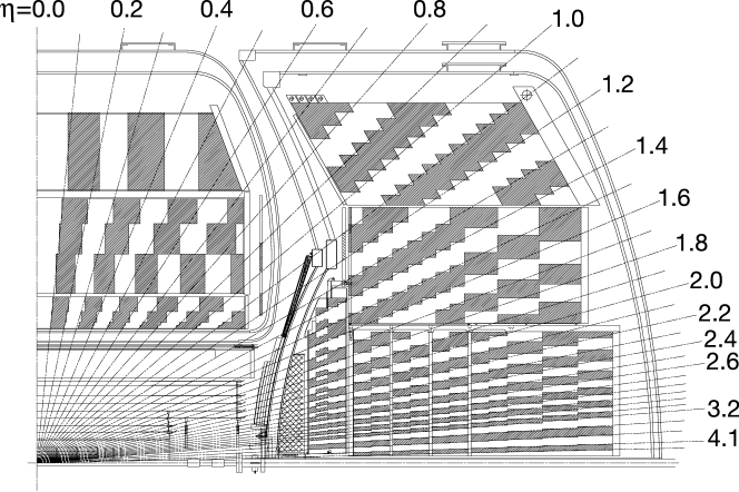
Figure 1: Side view of a quadrant of the D0 calorimeters showing the transverse and longitudinal segmentation. The alternating shading pattern indicates the cells for signal readout. The lines indicate the pseudorapidity intervals defined from the center of the detector. The inter-cryostat detector (ICD) is visible as a thin dark shaded tile between the cryostats, within $1.1<|{\eta_{\textnormal{det}}^{\textnormal{}}}|<1.4$.

As in any sampling calorimeter, incoming particles shower in absorber layers and ionize the active material (liquid argon). The electrons from the ionization are collected on anodes formed of carbon-coated epoxy films on G-10 substrates. Typical surface resistance when cold is $150-180\mskip 4.0mu plus 2.0mu minus 2.5mu\textnormal{${\rm M}\Omega/\Box$}$. The voltage across the typical $2.3\mskip 4.0mu plus 2.0mu minus 2.5mu\textnormal{mm}$ liquid argon gap is $\sim 2.0\mskip 4.0mu plus 2.0mu minus 2.5mu\textnormal{kV}$. At this field, the electron drift velocity in argon varies by about $0.3\%$ for a $1\%$ variation in electric field strength. Since the charge collection time of $\approx 450\mskip 4.0mu plus 2.0mu minus 2.5mu\textnormal{ns}$ is larger than the Tevatron bunch crossing time, only about two thirds of the electrons produced in the gap are used for charge measurement. As a result, changes in electric field in the gaps create a change in the detector response.

During the decade of Run II data collection, “dark” currents in the CC both with and without beam increased. The cause is attributed to a layer of uranium oxide on the surface of the CC absorber plates that is not present on the EC plates. This current increase is only seen in the CC. Migrating ions adhere to the surface of the oxide, creating a large potential across that material. A current through the layer could be caused by these large fields, and its flow could change the electric properties of the oxide, increasing its conductivity [20, 21]. This additional current draw through the resistance of the carbon-coated epoxy film results in a lower voltage across the argon gaps in the center of the CC than at the edges of the CC where high voltage connections are made to the resistive film. The spatial variation in collected charge (on the scale of 1%) is corrected by the offline calibration process. Calibrations had to be performed more frequently towards the end of Run II.

2.3 Calorimeter calibration

There are a number of steps for the conversion of a collected charge at a preamplifier into an amount of energy deposited in the calorimeter. We describe below the three steps applied concurrently with data taking: baseline subtraction, zero suppression, and electronics calibration.

To remove the baseline, the signal corresponding to a sampling occurring one bunch crossing earlier (by $396\mskip 4.0mu plus 2.0mu minus 2.5mu\textnormal{ns}$) is subtracted in analog circuitry before analog-to-digital conversion of the signal.

Due to residual uranium activity, the pedestal distribution around the baseline is asymmetric, with a larger tail towards more positive values, contributing to positive energies. Between stores, pedestal runs are taken to measure noise levels and to set zero suppression thresholds for each readout cell at $1.5$ times the RMS of the cell noise with no beam ($\sigma_{\textnormal{PED}}$). This zero suppression results in a net positive average cell energy, even in the absence of a particle flux, which is included in the jet energy scale corrections.

The stability and non-linear behavior of the electronics is measured and corrected by calibrating pulses at the inputs to the preamplifiers. This “NLC” calibration was done every two to three weeks during data taking. To extend the range of the analog to digital conversion, there are two gain paths ($\times 1$ and $\times 8$) in the readout electronics. The NLC runs calibrate both paths. There is a nonlinearity that remains due to saturation for extremely large signals, which becomes a significant effect when $\gtrsim 400\mskip 4.0mu plus 2.0mu minus 2.5mu\textnormal{GeV}$ of electromagnetic energy appears in a single calorimeter tower. No correction is applied for this saturation, but the results of the geant-based [22] calorimeter simulation are modified to describe this effect.

We use an algorithm called “T42” [23] to identify possible clusters of signal cells while suppressing isolated cells that are likely to arise from fluctuations in noise. Cells with an energy less than $2.5\,{\sigma_{\textnormal{PED}}}$ are considered to contain only noise and are rejected. Cells with an energy between $2.5$ and $4\,{\sigma_{\textnormal{PED}}}$ are considered only if adjacent to a cell with an energy at least $4\,{\sigma_{\textnormal{PED}}}$, since cells with little energy that are near cells with large signals are likely to measure the edges of a shower, while such low energy cells, when isolated, are likely due to noise. The T42 algorithm leads to a better rejection of noise cells, and hence improves jet energy resolution.

At periodic intervals, typically once per year but more frequently towards the end of Run II, specific data samples are taken and analyzed to provide a relative response calibration on a cell-by-cell basis uniform throughout the calorimeter. In each cell, the distribution of deposited energy, taken over all the events, is exponentially falling. The response of all the cells with the same $i_{\eta}$ value is adjusted so that the occupancy above a selected energy threshold is uniform in ${\phi}$. Events containing $Z\rightarrow{e^{+}e^{-}}$ decays were used to remove $i_{\eta}$ response variations within each module in the electromagnetic layers of the calorimeter and dijet events were used for the same purpose for the hadronic layers of the calorimeter. For the ICD detector, only ${\phi}$ uniformity is enforced by this procedure. The absolute response variation of ICD channels relative to the CC and EC is simulated in the physics analyses. This procedure corrects not only for the difference in response from the electronics, but also for the different amount of inactive material in front of the calorimeter cells, which varies with $i_{\eta}$ and $i_{{\phi}}$ [24]. Finally, the overall scale of the calorimeter calibration is fixed using $Z\rightarrow{e^{+}e^{-}}$ decay events and the known $Z$-boson mass $M_{Z}$ [25].

In most cells, the variations between these calibrations are of the order of 1%. The stability of the measured value of $M_{Z}$ after calibration was typically on the scale of a few hundred MeV or less in the CC, and somewhat larger in the EC. Figure 2 shows the measured mass of the $Z$ boson in $e^{+}e^{-}$ decays for a fraction of Run II data. This is the last fraction of the data for which a year passed between calibrations. After the summer of 2010, we began to calibrate more frequently because the rate of high voltage current increase was increasing with time, leading to a corresponding increase in the shifting of the observed $Z$ mass peak toward lower masses. In addition to energy, $\eta$ and $\phi$ dependences, electron energy is also corrected as a function of instantaneous luminosity.

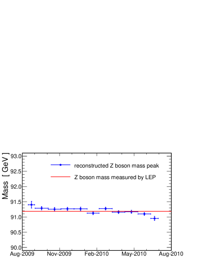
Figure 2: Typical variation with time of the mass of $Z$ boson reconstructed in the $e^{+}e^{-}$ final state for a fraction of the Run II data (reference value from Ref. [25]).

3 Reconstruction and identification of objects

This section describes the procedures used to reconstruct and identify the basic objects used to calibrate the jet energies.

3.1 Primary vertex

The first step is the reconstruction of vertices using prompt tracks. These vertices, referred to as “primary vertices” (PV), correspond to the locations of inelastic $p\bar{p}$ collisions. A significant fraction of the PVs are at $z$ positions considerably displaced from the center of the detector, and it is important to reconstruct the vertices with high efficiency and accuracy.

The reconstruction of vertices involves three steps: track selection, vertex fitting, and vertex selection. Tracks are selected with ${p^{\textnormal{}}_{\textnormal{T}}}\geq{0.5\mskip 4.0mu plus 2.0mu minus 2.5mu\textnormal{$\textnormal{GeV}$}}$, with at least two SMT hits, and transverse impact parameter (with respect to the beam axis) smaller than three times its uncertainty [27]. Starting from the track with highest $p^{\textnormal{}}_{\textnormal{T}}$, the tracks are clustered based on the $z$ position of their closest approack to the beam axis. Tracks are added to the cluster if they are within $2\mskip 4.0mu plus 2.0mu minus 2.5mu\textnormal{cm}$ in $z$ from the $z$ position of the seed track. By constraining all tracks in a cluster to a common vertex, the track parameters and vertex position are recalculated using a Kalman Filter technique [27, 28]. The algorithm is repeatedly applied to the remaining tracks to build a list of vertex candidates.

The presence of multiple $p\bar{p}$ interactions during the bunch crossing typically leads to the reconstruction of several vertices in the event. For each reconstructed vertex, the probability that it originates from a soft $p\bar{p}$ inelastic interaction (“minimum bias probability”) is computed from the tracks associated with the vertex, making use of a template of the distribution of $\log_{10}({p^{\textnormal{}}_{\textnormal{T}}})$. The vertex with the lowest minimum bias probability is chosen as the hard-scatter PV. To ensure that a hard-scatter vertex of high quality is selected, it is required to be reconstructed from at least three tracks, and to be located at $\left|{{z_{\textnormal{PV}}}}\right|\leq{50\mskip 4.0mu plus 2.0mu minus 2.5mu\textnormal{cm}}$.

3.2 Calorimeter objects

The jet energy calibration procedure relies on calorimeter objects (photons, jets, and missing transverse energy), which are reconstructed starting from the individual calorimeter cells. This section presents a discussion of the reconstruction and identification algorithms used for the relevant calorimeter objects.

3.2.1 Electromagnetic clusters

EM clusters are formed from the towers in electromagnetic calorimeter which have ${p^{\textnormal{}}_{\textnormal{T}}}>{500\mskip 4.0mu plus 2.0mu minus 2.5mu\textnormal{$\textnormal{MeV}$}}$ (“seed towers”) starting from the highest $p^{\textnormal{}}_{\textnormal{T}}$ tower. Neighboring towers are added if they have ${p^{\textnormal{}}_{\textnormal{T}}}>{50\mskip 4.0mu plus 2.0mu minus 2.5mu\textnormal{$\textnormal{MeV}$}}$ and if they are within ${\Delta\mathcal{R}}=\sqrt{(\Delta\eta)^{2}+(\Delta\phi)^{2}}<0.3$ of the seed tower in the CC, or within a cone of radius $10\mskip 4.0mu plus 2.0mu minus 2.5mu\textnormal{cm}$ in the third layer of the EM calorimeter in the EC. Such preclusters are used as starting points for the final clusters if their energy exceeds $1\mskip 4.0mu plus 2.0mu minus 2.5mu\textnormal{GeV}$. Any EM tower within ${\Delta\mathcal{R}}<0.4$ is added, and the center of the final cluster is defined by the energy-weighted mean of its cells in the third layer of the EM calorimeter.

3.2.2 Jets

Jets resulting from the hard $p\bar{p}$ scatter usually involve a large number of particles that deposit energy in numerous calorimeter cells. The reconstruction of jets, either from stable particles or calorimeter towers, involves a clustering algorithm to assign particles or calorimeter towers to jets. We define jets using the Run II Midpoint cone algorithm [29], which is a fixed-cone algorithm. The jet centroid is defined as $(y_{\textnormal{jet}},{\phi}_{\textnormal{jet}})$ [17], and objects are clustered if their distance relative to the jet axis, ${\Delta\mathcal{R}}=\sqrt{(y_{\textnormal{obj}}-y_{\textnormal{jet}})^{2}+({\phi}_{\textnormal{obj}}-{\phi}_{\textnormal{jet}})^{2}}<{\mathcal{R}_{\textnormal{cone}}}$, where ${\mathcal{R}_{\textnormal{cone}}}$ is the cone radius. Jet energy scale corrections and uncertainties have been determined for ${\mathcal{R}_{\textnormal{cone}}}=0.5$ and $0.7$.

The reconstruction of jets in the detector involves a number of steps. First, pseudo-projective calorimeter towers are reconstructed by adding the four-momenta of their associated calorimeter cells that are above threshold, treating each cell four-momentum as massless. The momentum of each cell is defined with respect to the PV, as reconstructed by the tracking system. As a result, calorimeter towers are treated as massive objects. In a second step, the calorimeter towers with ${p^{\textnormal{}}_{\textnormal{T}}}\geq{1\mskip 4.0mu plus 2.0mu minus 2.5mu\textnormal{$\textnormal{GeV}$}}$ are used as seeds to find pre-clusters, which are formed by adding neighboring towers within ${\Delta\mathcal{R}}<0.3$ with respect to the seed tower. The pre-clustering step reduces the number of seeds passed to the main algorithm, keeping the analysis computationally feasible. A cone of radius ${\mathcal{R}_{\textnormal{cone}}}$ is formed around each pre-cluster, centered at its centroid, and a new proto-jet center is computed using the $E$-scheme:

$$\begin{split}p^{\mu}&=\left(E,\vec{p}\right)=\sum_{i}\left(E_{i},\vec{p}_{i}\right),\\ y&=\frac{1}{2}\ln\left(\frac{E+p_{z}}{E-p_{z}}\right),\\ {\phi}&=\tan^{-1}\left(\frac{p_{y}}{p_{x}}\right),\\ {p^{\textnormal{}}_{\textnormal{T}}}&=\sqrt{p_{x}^{2}+p_{y}^{2}},\end{split}$$ (1)

where the sums are over all towers (or, in MC, particles or partons) contained in the cone. The proto-jet center is modified to the location ($y,\phi$). The direction of the resulting four-vector is used as the center point for a new cone. When the proto-jet four-momentum does not coincide with the cone axis, the procedure is repeated using the new axis as the center point until a stable solution is found. The maximum number of iterations is 50 and the solution is considered to be stable if the difference in ${\Delta\mathcal{R}}$ between two iterations is smaller than 0.001. In the rare cases of bistable solutions, the last iteration is retained. Any proto-jets falling below the threshold of ${p^{\textnormal{}}_{\textnormal{T}}}<{3\mskip 4.0mu plus 2.0mu minus 2.5mu\textnormal{$\textnormal{GeV}$}}$ are discarded.

The presence of a threshold requirement on the cluster seeds introduces a dependency on infrared and collinear radiation. The sensitivity to soft radiation is reduced by the addition of $p^{\textnormal{}}_{\textnormal{T}}$-weighted midpoints between pairs of proto-jets and repeating the iterative procedure for these midpoint seeds. The last step of the algorithm involves splitting and merging to treat overlapping proto-jets, i.e. proto-jets separated by a distance of ${\Delta\mathcal{R}}<2{\mathcal{R}_{\textnormal{cone}}}$. Overlapping proto-jets are merged into a single jet if more than $50\%$ of the $p^{\textnormal{}}_{\textnormal{T}}$ of the lower-energy jet is contained in the overlap region. Otherwise, the energy of each cell in the overlap region is assigned to the nearest jet. Finally, the four-momentum of the jet is recomputed using the $E$-scheme and jets with ${p^{\textnormal{}}_{\textnormal{T}}}<{6\mskip 4.0mu plus 2.0mu minus 2.5mu\textnormal{$\textnormal{GeV}$}}$ are discarded.

The jet algorithm described above can also be applied to stable particles in MC events. Stable particles are defined as those reaching the D0 detector volume. All stable particles produced in the interaction are considered, including not only the ones from the hard scattering process, but also from the underlying event. The exceptions are muons and neutrinos that are not included. Jets clustered from the list of considered stable particles (particle jets) are used to define the particle level jet energy. The goal of the jet energy scale calibration procedure is to correct the measured energy of calorimeter jets to the particle level.

Small modifications in the jet-finding algorithm (pre-cluster selection and merging/splitting treatment) are applied to Run IIb data to meet conditions with higher instantaneous luminosity.

3.2.3 Missing transverse energy

The missing energy in the transverse plane ${{\not\!\!{E^{\textnormal{cal}}_{\textnormal{T}}}}}$ is defined by its components in $x$ and $y$ projections:

$${\not\!\!E_{x}^{\textnormal{cal}}}=-p_{x}^{\textnormal{vis}}\quad\text{and}\quad{\not\!\!E_{y}^{\textnormal{cal}}}=-p_{y}^{\textnormal{vis}},$$

where $p_{x/y}^{\textnormal{vis}}$ are the components of the visible transverse momentum, computed from all the calorimeter cells that pass the T42 selection:

$$p_{x/y}^{\textnormal{vis}}=\sum_{i\in\textnormal{cells}}p_{x/y,i}.$$

For the measurements presented in this article, CH cells are excluded from ${\not\!\!{E^{\textnormal{cal}}_{\textnormal{T}}}}$ due to their limited energy resolution.

The ${\not\!\!{E^{\textnormal{}}_{\textnormal{T}}}}$ is adjusted for energy scale corrections that are applied to reconstructed electromagnetic objects. The corrections of electromagnetic objects that pass the photon identification criteria described in Sec. 3.3 are subtracted:

$${\not\!\!E}_{x/y}={\not\!\!E_{x/y}^{\textnormal{cal}}}-\sum_{i\in\textnormal{photons}}\left({E_{x/y,i}^{\gamma,\textnormal{corr}}-E_{x/y,i}^{\gamma,\textnormal{uncorr}}}\right).$$ (2)

3.3 Photon identification criteria

A cluster in the electromagnetic calorimeter is identified as a photon if it satisfies the following criteria:

• The object is an isolated electromagnetic cluster.

• The object is reconstructed in the central region (${\left|{{\eta_{\textnormal{det}}^{\textnormal{}}}}\right|}<1.0$) and in the fiducial regions of the calorimeter (objects near module boundaries are excluded).

• The fraction of energy deposited in the electromagnetic part of the calorimeter ($f_{\rm EM}$) must be greater than $0.96$.

• The probability to have a spatially matched track must be less than $0.1\%$.

• The cluster is isolated in the calorimeter in a cone of radius ${\Delta\mathcal{R}}=0.4$ by $\left[{E_{\textnormal{tot}}(0.4)-E_{\textnormal{EM}}(0.2)}\right]/E_{\textnormal{EM}}(0.2)<0.07$, where $E_{\textnormal{tot}}(0.4)$ $[E_{\textnormal{EM}}(0.2)]$ is the total [EM only] energy in the cone of ${\Delta\mathcal{R}}=0.4$ [$0.2$].

• The scalar sum of the $p^{\textnormal{}}_{\textnormal{T}}$ of all tracks originating from the $p\bar{p}$ hard-scatter vertex in an annulus of $0.05<{\Delta\mathcal{R}}<0.7$ around the EM cluster must be less than $1.0\mskip 4.0mu plus 2.0mu minus 2.5mu\textnormal{$\textnormal{GeV}$}$. Tracks are considered if their transverse momentum exceeds $0.4\mskip 4.0mu plus 2.0mu minus 2.5mu\textnormal{$\textnormal{GeV}$}$ and if their distance of closest approach in $z$ to the vertex is less than $1\mskip 4.0mu plus 2.0mu minus 2.5mu\textnormal{cm}$.

• The square of the energy-weighted cluster width in ${r}\times{\phi}$ in the third layer of the EM calorimeter must be less than $14\mskip 4.0mu plus 2.0mu minus 2.5mu\textnormal{$\textnormal{cm}^{2}$}$.

• The weighted sum of energy depositions in the CPS strips around the line connecting the PV and EM cluster must correspond to a single EM object.

This set of criteria is further referred to as a “tight photon selection”, and an object satisfying these criteria as a “tight photon”. For the purpose of background studies, namely the measurement of contamination from dijet events where one of the jets is misidentified as a photon, two additional slections with less stringent criteria are considered. A loose photon selection follows the same criteria, but the requirement on the scalar sum of transverse momenta of associated tracks is removed, and no information from the preshower detector is used. A medium selection is also based on the tight one, but the cut on the scalar sum of transverse momenta of associated tracks is relaxed to $2\mskip 4.0mu plus 2.0mu minus 2.5mu\textnormal{$\textnormal{GeV}$}$ and the outer radius of the annulus is reduced to 0.4.

3.4 Jet identification criteria

Jets reconstructed in the calorimeter must satisfy the following selection criteria:

• The fraction $f_{\rm EM}$ must be greater than $0.05$ and less than $0.95$. Jets in the forward region (${\left|{{\eta_{\textnormal{det}}^{\textnormal{}}}}\right|}>2.5$) must satisfy $f_{\rm EM}>0.04$. This requirement is not enforced on jets in ICR.

• The fraction of energy in the coarse hadronic calorimeter ($f_{\rm CH}$) must be less than $0.44$ for jets with ${\left|{{\eta_{\textnormal{det}}^{\textnormal{}}}}\right|}<0.8$, less than $0.46$ for jets in the endcap region $1.5<{\left|{{\eta_{\textnormal{det}}^{\textnormal{}}}}\right|}<2.5$, and less than 0.4 for all other jets. Exception is the jets in the region $0.85<{\left|{{\eta_{\textnormal{det}}^{\textnormal{}}}}\right|}<1.25$, which are allowed to have $f_{\rm CH}<0.6$, if at the same time the number of cells that contain $90\%$ of the jet energy is less than 20. The requirement on $f_{\rm CH}$ is aimed at removing jets dominated by noise originating in the coarse hadronic part of the calorimeter.

• The jet must be “confirmed” by the independent readout of calorimeter energies in the Level 1 trigger, i.e., the energy of the trigger towers inside a cone of ${\Delta\mathcal{R}}=0.5$ around the jet axis must be at least 50% of the energy of the jet as reconstructed by the precision readout. This condition, progressively loosened to 10% for forward jets (${\eta_{\textnormal{det}}^{\textnormal{}}}>1.4$) and soft jets (${p^{\textnormal{}}_{\textnormal{T}}}<{15\mskip 4.0mu plus 2.0mu minus 2.5mu\textnormal{$\textnormal{GeV}$}}$), suppresses spurious jets due to calorimeter readout noise.

4 Overview of jet energy scale determination

The evolution from the colored parton to a jet of hadrons is dominated by low energy processes that are not calculable perturbatively by Quantum Chromodynamics (QCD), and lead to large variations in the composition of a jet. The energy calibration of a jet is fundamentally different than for any other object in particle physics, since it does not correspond to a single well-defined particle such as an electron or a muon. The measured energy of a jet is not fully correlated to energy of its progenitor parton due to two effects: the parton-to-hadron fragmentation that leads to the creation of the jet, and the interaction of the final state hadrons with the detector.

The goal of the jet energy scale correction is to relate, on average, the jet energy measured in the detector to the energy of the final state particle jet. Because jets are composite objects, the algorithm used to reconstruct them defines the particle jet to which we calibrate. We employ a calibration methodology related, to but modified from, Ref. [11]. The particle jet energy $E^{\textnormal{ptcl}}_{\textnormal{}}$ can be related to the measured energy $E^{\textnormal{meas}}_{\textnormal{}}$ of the reconstructed jet via:

$${E^{\textnormal{ptcl}}_{\textnormal{}}}=\frac{{E^{\textnormal{meas}}_{\textnormal{}}}-E_{\textnormal{O}}}{R\cdot S},$$ (3)

where:

• $E_{\textnormal{O}}$ represents an offset energy, which includes several contributions. Noise arises from electronics and radioactive decay of the uranium absorber. Additional in-time $p\bar{p}$ interactions and those from previous crossings, termed “pile-up”, also contribute. The underlying event, defined as the energy contributed by the proton and antiproton constituents not participating directly in the hard interaction (“spectators”), is considered to be part of the high-$p^{\textnormal{}}_{\textnormal{T}}$ event and therefore not subtracted. The offset energy depends on the jet cone radius (${\mathcal{R}_{\textnormal{cone}}}$), jet detector pseudorapidity ($\eta_{\textnormal{det}}^{\textnormal{}}$), number of reconstructed primary vertices (${n_{\textnormal{PV}}}$), and instantaneous luminosity ($\mathcal{L}$).

• $R$ represents the response of the calorimeter to the energy of the particles comprising the jets. Its value is generally smaller than unity, primarily because response to hadrons, particularly to charged pions, is lower than response to electrons, that is set to unity by the calibration (Sec. 2.3). The ratio of responses, $e/\pi$, has a significant dependence on particle energy. Significant energy is also lost in non-sampled material before the calorimeter, and in non-instrumented regions between calorimeter modules. The ICR region is poorly sampled and this leads to energy scale variations. For these reasons, the jet response is a function of jet energy and, particularly in the ICR region, of $\eta_{\textnormal{det}}^{\textnormal{}}$. A small but non-negligible variation occurs for different cone algorithms, since particles near the jet core tend to have higher energy and thus higher response than particles near the jet boundary.

• The function $S$ represents corrections for the showering of particles in the detector. Due to the cone size ${\mathcal{R}_{\textnormal{cone}}}$ and the calorimeter cell size, energy from particles originating within a jet can spread to cells outside the cone radius. This is not to be confused with parton showering during fragmentation, that is a process occurring prior to interaction with the detector. Conversely, energy may be deposited in cells inside this boundary that originated from particles that do not belong to the particle jet (e.g., due to showering effects in the calorimeter, or to the magnetic field changing the direction of particles outside of the jet cone). Typically, the net correction is close to unity. It depends strongly on ${\mathcal{R}_{\textnormal{cone}}}$ and $\eta_{\textnormal{det}}^{\textnormal{}}$, and only mildly on jet energy.

We refer to the terms on the right-hand side of Eq. 3 as true values of the corrections. In practice, the $E_{\textnormal{O}}$, $R$ and $S$ corrections that we measure represent only estimators of the true corrections and may be affected by a number of biases. We explicitly correct for these biases to ensure that the mean particle jet energy is recovered.

4.1 True corrections

We first examine the definition of the true corrections discussed in the previous section. Here, we assume that no multiple interactions or pile-up are present, and only the hard $p\bar{p}$ interaction produces the jet. The particle jet energy is defined as the sum of energies of all stable particles belonging to the particle jet as defined in Sec. 3.2.2:

$${E^{\textnormal{ptcl}}_{\textnormal{}}}=\sum_{i\in\textnormal{ptcljet}}E_{i}.$$ (4)

The measured jet energy receives contributions from particles both inside and outside the particle jet, as well as the offset energy:

$${E^{\textnormal{meas}}_{\textnormal{}}}=\sum_{i\in\textnormal{ptcljet}}{E^{\textnormal{meas}}_{\textnormal{$i$}}}f_{i}+\sum_{i\notin\textnormal{ptcljet}}{E^{\textnormal{meas}}_{\textnormal{$i$}}}f_{i}+E_{\textnormal{O}},$$ (5)

where $E^{\textnormal{meas}}_{\textnormal{$i$}}$ is the visible calorimeter energy from particle $i$, and $f_{i}$ is the fraction of such energy contained within the calorimeter jet cone. After subtracting the true offset energy $E_{\textnormal{O}}$, we obtain, by definition, the energy inside the calorimeter jet cone in the absence of any noise, pile-up or multiple interaction effects.

We define the true response correction to be the ratio of visible energy for particles from the particle jet divided by the energy of the incident particle jet (given by Eq. 4):

$$R=\frac{\sum_{i\in\textnormal{ptcljet}}{E^{\textnormal{meas}}_{\textnormal{$i$}}}}{{E^{\textnormal{ptcl}}_{\textnormal{}}}}.$$ (6)

This definition includes all the constituents of the particle jet, regardless of whether their energy is deposited within the cone radius of the reconstructed jet.

To satisfy Eq. 3, the true showering correction is defined as:

$$S=\frac{\sum_{i\in\textnormal{ptcljet}}{E^{\textnormal{meas}}_{\textnormal{$i$}}}f_{i}+\sum_{i\notin\textnormal{ptcljet}}{E^{\textnormal{meas}}_{\textnormal{$i$}}}f_{i}}{\sum_{i\in\textnormal{ptcljet}}{E^{\textnormal{meas}}_{\textnormal{$i$}}}}.$$ (7)

This represents a correction from the visible energy inside the calorimeter jet cone, resulting from particles both inside and outside the particle jet, to the total visible energy resulting from the particle jet, whose cone may differ from the one of the calorimeter jet.

4.2 Estimated corrections

The jet offset, response and showering corrections can be estimated in data, and are represented by $\hat{E}_{\textnormal{O}}$, $\hat{R}$ and $\hat{S}$. Ideally, the corrected jet energy would be given by Eq. 3, with the true corrections replaced by the estimated corrections:

$${\hat{E}}^{\textnormal{corr}}=\frac{{E^{\textnormal{meas}}_{\textnormal{}}}-\hat{E}_{\textnormal{O}}}{\hat{R}\cdot\hat{S}}.$$ (8)

Since the estimated corrections suffer from biases, the corrected jet energy as given by Eq. 8 can differ by several percent from $E^{\textnormal{ptcl}}_{\textnormal{}}$. We therefore determine additional corrections using Monte Carlo (MC) samples to remove biases of the estimated corrections. The final jet energy correction is given by the modified expression:

$${E^{\textnormal{corr}}_{\textnormal{}}}=\frac{({E^{\textnormal{meas}}_{\textnormal{}}}-\hat{E}_{\textnormal{O}}){k_{\textnormal{O}}^{\textnormal{}}}}{\hat{R}\;{k_{\textnormal{R}}^{\textnormal{}}}\,\hat{S}},$$ (9)

where $k_{\textnormal{O}}^{\textnormal{}}$ and $k_{\textnormal{R}}^{\textnormal{}}$ represent the bias corrections to offset and response, respectively. As will be discussed in Sec. 11, $\hat{S}$ is a priori an unbiased estimator of the true showering correction, and no bias correction is required. After these corrections, Eq. 9 provides, on average, the unbiased energy of the particle jet.

4.3 Biases from the sample composition

The corrections to data and MC simulation are extracted independently, although the procedure is similar. All corrections are determined on average in the sense that they are parametrized on only a few characteristic properties of the jet.

Jets have different characteristics according to whether they originate from a light quark, $c$ quark, $b$ quark, or a gluon (the “parton flavor” of the jet). The jet energy scale correction outlined above considers a mixture of jets with parton flavors produced by the physical process used in the calibration, namely ${\gamma}+\textnormal{jet}$. This correction calibrates samples composed of a mixture of jets with parton flavor content similar to ${\gamma}+\textnormal{jet}$ production processes. In samples with different composition, this correction will generally have a bias depending on the partonic content of the sample.

The method described in this article uses both ${\gamma}+\textnormal{jet}$ and dijet events. This yields the extraction of two energy scales, appropriate for the analysis of data samples with composition similar to the ${\gamma}+\textnormal{jet}$ and dijet processes, respectively.

Even without knowledge of the precise composition of the data sample, it is still possible to perform measurements with the available energy scale by comparing with the MC, provided that the simulation describes the features and biases of jets with different parton flavor, i.e., their calorimeter response. Section 14 describes an improvement to this description based on the calibration of the simulated response to single particles inside a jet using data, and Sec. 15 presents a further correction to improve the description of simulated jets.

5 Overview of response correction

The response correction ($R$) is numerically the largest correction in the jet energy scale calibration procedure, since it accounts for a number of sizable instrumental effects that influence the jet energy measurement. First, particles emerging from the hard scattering interact with the material before the calorimeter and lose a fraction of their energy, which can be significant for low momentum particles. Furthermore, charged particles are deflected in the magnetic field and, depending on their $p^{\textnormal{}}_{\textnormal{T}}$, can potentially fail to reach the calorimeter (e.g., charged particles in the central rapidity region with ${p^{\textnormal{}}_{\textnormal{T}}}<{0.3\mskip 4.0mu plus 2.0mu minus 2.5mu\textnormal{$\textnormal{GeV}$}}$). Most particles reaching the calorimeter (except for muons and neutrinos, which constitute, on average, a small fraction of the jet energy) are fully absorbed and their deposited energy is transformed into a signal.

The D0 calorimeter is non-compensating: it has a higher and more linear response to electromagnetic particles ($e^{\pm},{\gamma}$) than to hadrons ($e/h>1$). The energy dependence of the response to hadrons is nearly logarithmic as a result of the slow rise of the fraction of $\pi^{0}$ mesons produced as a function of the hadron energy during hadronic shower development [30]. Zero suppression can also significantly contribute to the non-linearity of response to hadrons, especially at low jet momentum. Finally, calorimeter module-to-module inhomogeneities or poorly instrumented regions (e.g., the ICR) can result in significant distortions to the measured jet energy.

Some of these instrumental effects (e.g., the calorimeter response to hadrons) are difficult to model accurately in the MC simulation. As a result, data and MC have a different response to jets, requiring response corrections to be determined separately for data and MC. While in MC it is a priori possible to compute the response correction exactly by comparing the measured jet energy to the particle jet energy, this information is not available in data. The Missing $E^{\textnormal{}}_{\textnormal{T}}$ Projection Fraction (MPF) method [11, 31] has been developed to measure the calorimeter response to jets in data. We use this method to measure the jet response in both data and MC. Applying the MPF method to MC, where the true jet response is known, allows an evaluation of the biases of the method and development of suitable correction procedures to be applied to data. In the next sections we give an overview of the MPF method, followed by the discussion of the expected biases and the corresponding corrections. Finally, we outline the strategy to determine the jet energy response correction.

5.1 Missing $E^{\textnormal{}}_{\textnormal{T}}$ Projection Fraction method

We consider a two-body process $X+\textnormal{jet}$, where $X$ ($\gamma$, $Z$ boson, or jet) is referred to as the “tag object”, and the jet is the “probe object” whose response we are estimating. The MPF method can be used to estimate the calorimeter response of the probe jet relative to the response of the tag object. This method is also exploited to intercalibrate the response of different calorimeter regions.

At the particle level, the transverse momenta of the tag object ($\vec{p}_{\textnormal{T\,tag}}$) and of the hadronic recoil ($\vec{p}_{\textnormal{T\,recoil}}$) are balanced due to overall transverse momentum conservation in a given event:

$$\vec{p}_{\textnormal{T\,tag}}+\vec{p}_{\textnormal{T\,recoil}}=0.$$ (10)

The probe jet is part of the hadronic recoil, but may not constitute the entire hadronic recoil. In a calorimeter, the responses of the tag object ($R_{\textnormal{tag}}$) and the hadronic recoil ($R_{\textnormal{recoil}}$) might be different, which results in a transverse momentum imbalance as measured by the calorimeter:

$$\vec{p}^{\,\textnormal{meas}}_{\textnormal{T\,tag}}+\vec{p}^{\,\textnormal{meas}}_{\textnormal{T\,recoil}}=-{{\not\!\!\vec{E}}^{\textnormal{}}_{\textnormal{T}}}{},$$ (11)

where $\vec{p}^{\,\textnormal{meas}}_{\textnormal{T\,tag}}=R_{\textnormal{tag}}\,\vec{p}_{\textnormal{T\,tag}}$ is the measured transverse momentum of the tag object, $\vec{p}^{\,\textnormal{meas}}_{\textnormal{T\,recoil}}=R_{\textnormal{recoil}}\,\vec{p}_{\textnormal{T\,recoil}}$ is the measured transverse momentum of the hadronic recoil, and ${\not\!\!\vec{E}}^{\textnormal{}}_{\textnormal{T}}$ is the missing transverse energy measured in the event (see Sec. 3.2.3).

From Eqs. 10 and 11 we derive the following expression:

$$\frac{R_{\textnormal{recoil}}}{R_{\textnormal{tag}}}=1+\frac{{{\not\!\!\vec{E}}^{\textnormal{}}_{\textnormal{T}}}{}\cdot\vec{n}_{\textnormal{T\,tag}}}{{p^{\textnormal{meas}}_{\textnormal{T\,tag}}}},$$ (12)

which shows that the response of the hadronic recoil relative to the response of the tag object can be estimated from the projection of ${\not\!\!\vec{E}}^{\textnormal{}}_{\textnormal{T}}$ onto the direction of the tag object in the transverse plane, $\vec{n}_{\textnormal{T\,tag}}$.

In the ideal case, where the probe jet is identical to the hadronic recoil, we can replace $R_{\textnormal{recoil}}$ in Eq. 12 by the jet response, $R$. However, the presence of additional jets in the event, some of which might not even be reconstructed, make this idealized situation impossible to achieve in practice. By requiring exactly two reconstructed objects (tag and probe) back-to-back in azimuthal angle, it is possible to significantly improve the approximation that $R\approx R_{\textnormal{recoil}}$. Residual effects at the percent level remain and are subsequently corrected (see Sec. 10). To avoid confusion with the true response of the particle jet ($R$), we will refer to the jet response estimated with the MPF method as $R_{\textnormal{MPF}}^{\textnormal{sample}}$, where the superscript will be used to indicate which sample has been used to estimate the response. This information is important, since the MPF response depends on the sample used (e.g., via the parton flavor composition, color flow, etc.). It also depends on the corrections applied to the energy of the tag object, which are propagated into ${\not\!\!{E^{\textnormal{}}_{\textnormal{T}}}}$.

5.1.1 Resolution bias

Eq. 12 attributes the average imbalance in transverse momentum in the event, ${\not\!\!{E^{\textnormal{}}_{\textnormal{T}}}}$, to differences in calorimeter response between the tag and probe objects. For a precise determination of this relative response it is important to eliminate all sources of imbalance that are unrelated to calorimeter response.

In particular, when measuring $R_{\textnormal{recoil}}/R_{\textnormal{tag}}$ in bins of $p^{\textnormal{meas}}_{\textnormal{T\,tag}}$, there is a possibility of a significant imbalance (${\not\!\!{E^{\textnormal{}}_{\textnormal{T}}}}$) arising purely from resolution effects. The dominant effect arises from the finite calorimeter energy resolution coupled with a steeply falling jet $p^{\textnormal{}}_{\textnormal{T}}$ spectrum. In this case, each $p^{\textnormal{meas}}_{\textnormal{T\,tag}}$ bin tends to contain on average more upward fluctuations from lower $p^{\textnormal{}}_{\textnormal{T}}$ than downward fluctuations from higher $p^{\textnormal{}}_{\textnormal{T}}$. As a result, there is positive bias in the average $p^{\textnormal{meas}}_{\textnormal{T\,tag}}$ that translates into an artificial source of ${\not\!\!{E^{\textnormal{}}_{\textnormal{T}}}}$ imbalance in the event. We refer to this effect as “resolution bias”. Because this bias depends on the jet energy resolution, its size also depends on $\eta_{\textnormal{det}}^{\textnormal{}}$ of the jet.

This bias can be precisely estimated if the tag object $p^{\textnormal{}}_{\textnormal{T}}$ spectrum and $p^{\textnormal{}}_{\textnormal{T}}$ resolution are known. The expected resolution bias in the transverse momentum of the tag photon in ${\gamma}+\textnormal{jet}$ events is much smaller than $1\%$ [41] and can thus be neglected. In contrast, the expected resolution bias in the transverse momentum of the tag jet in dijet events can be much larger [4] and needs to be explicitly corrected. To evaluate this correction a detailed numerical calculation is performed taking into account the measured $p^{\textnormal{}}_{\textnormal{T}}$ spectrum in data dijet events as a function of $\eta_{\textnormal{det}}^{\textnormal{}}$ of the probe jet and a precise measurement of the jet energy resolution for a jet in the calorimeter [4]. This correction procedure has been validated in MC and verified to properly correct the bias, within an uncertainty of $0.5\%-1.0\%$.

5.1.2 Absolute MPF response

The absolute MPF jet response is estimated from Eq. 12 using ${\gamma}+\textnormal{jet}$ events with a jet in the central calorimeter region ($|{\eta_{\textnormal{det}}^{\textnormal{}}}|<0.4$), assuming that the measured transverse momentum of the photon is converted to the particle level ($p^{\textnormal{}}_{\textnormal{T{$\gamma$}}}$) by the EM energy scale corrections. In this case the photon response $R_{{\gamma}}=1$, and Eq. 12 can be rewritten as:

$${R_{\textnormal{MPF}}^{\textnormal{{${\gamma}+\textnormal{jet}$}}}}=1+\frac{{{\not\!\!\vec{E}}^{\textnormal{}}_{\textnormal{T}}}\cdot\vec{n}_{\textnormal{T{$\gamma$}}}}{{p^{\textnormal{}}_{\textnormal{T{$\gamma$}}}}}.$$ (13)

The most important dependence of the jet response is on the jet energy. As discussed in Sec. 5.1.1, the jet energy resolution causes a bias in the estimated jet response. Therefore, to measure the energy dependence of the jet response with minimal impact from resolution effects we use the jet energy estimator $E^{\prime}$, defined as:

$${E^{\prime}}={p^{\textnormal{}}_{\textnormal{T{$\gamma$}}}}\cosh(\eta),$$ (14)

where $\eta$ is the jet pseudorapidity with respect to the reconstructed $p\bar{p}$ collision vertex in the event. The estimator $E^{\prime}$ is calculated using the photon transverse momentum and the jet direction, which are measured more precisely than the jet energy itself. It is strongly correlated with the particle level jet energy. We also use the quantity $p^{\prime}_{\textnormal{T}}$, defined as

$${p^{\prime}_{\textnormal{T}}}={E^{\prime}}/\cosh({\eta_{\textnormal{det}}^{\textnormal{}}}),$$ (15)

where $\eta_{\textnormal{det}}^{\textnormal{}}$ is the detector pseudorapidity of the probe jet [17].

The energy dependence of the jet response is well described by a quadratic logarithmic function [4, 11]:

$$R\left({E^{\prime}}\right)={c_{0}}+{c_{1}}\log({E^{\prime}}/E_{0})+{c_{2}}\log^{2}({E^{\prime}}/E_{0}),$$ (16)

where $E_{0}$ is a constant and $c_{i}$ ($i=0,1,2$) are free parameters to be determined. A detailed description of the measurement of the jet absolute response is given in Sec. 8.

5.1.3 Relative MPF response: pseudorapidity dependence

Even after individual cells are calibrated, the D0 calorimeter exhibits a non-uniform response to jets as a function of ${\eta_{\textnormal{det}}^{\textnormal{}}}$. The jet response is rather uniform within the CC region; however, in data (MC) the EC response is $\sim 15\%$ $(10\%)$ lower than the CC response. An important contribution to this non-uniformity arises from the poorly instrumented ICR region ($1.1<{\left|{{\eta_{\textnormal{det}}^{\textnormal{}}}}\right|}<1.5$). As discussed in Sec. 2.2, a substantial amount of energy in this region is lost in the solenoid, cryostat walls, module end-plates, and support structures. As a result, the ICR region has the largest deviation in energy dependence of response respect to the central calorimeter. In the $1.2<{\left|{{\eta_{\textnormal{det}}^{\textnormal{}}}}\right|}<1.4$ region, the calorimeter lacks an electromagnetic section and the total depth drops below $6\lambda_{\textnormal{int}}$. The goal of the relative MPF response correction is to address this effect in such a way that the corrected MPF response is uniform for the entire calorimeter, independent of $\eta_{\textnormal{det}}^{\textnormal{}}$. Since different calorimeter regions have different energy dependence of the response, this correction is not only a function of $\eta_{\textnormal{det}}^{\textnormal{}}$, but also of energy.

To express the dependence on $\eta_{\textnormal{det}}^{\textnormal{}}$, the relative MPF response correction, ${F_{\eta}^{\textnormal{}}}$, as defined in detail in Sec. 9.1, is estimated using samples of ${\gamma}+\textnormal{jet}$ and dijet events (see ). The former sample allows a direct and consistent derivation of the MPF response relative to the central calorimeter, with a normalization of ${F_{\eta}^{\textnormal{}}}$ to unity for the central jets ($|{\eta_{\textnormal{det}}^{\textnormal{}}}|<0.4$). The dijet sample provides the additional statistics required to measure this correction in fine bins of $\eta_{\textnormal{det}}^{\textnormal{}}$ and up to much higher energies than the ${\gamma}+\textnormal{jet}$ sample can reach. By combining these two different samples, we reduce both statistical and systematic uncertainties of the relative response correction.

The ${F_{\eta}^{\textnormal{}}}$ factors are found from a global fit to data in all ${\eta_{\textnormal{det}}^{\textnormal{}}}$ bins simultaneously. The dijet sample has a different composition of quark- and gluon-initiated jets as compared to ${\gamma}+\textnormal{jet}$ events (Sec. 16). For this reason, the responses in the two samples differ, albeit having the same form of energy dependence in a given ${\eta_{\textnormal{det}}^{\textnormal{}}}$ (see Sec. 9.1.3). From the global fit, the correction factors for the ${\gamma}+\textnormal{jet}$ and dijet samples, ${F_{\eta}^{\textnormal{{${\gamma}+\textnormal{jet}$}}}}$ and ${F_{\eta}^{\textnormal{dijet}}}$, are available separately. The ${F_{\eta}^{\textnormal{dijet}}}$ factors are used later to derive jet energy scale corrections for dijet events, described in Sec. 16.

5.2 MPF response biases

As discussed in the previous section, an estimate of the absolute jet response can be obtained by applying the MPF method to selected ${\gamma}+\textnormal{jet}$ events (free from the resolution bias), so that $\hat{R}={R_{\textnormal{MPF}}^{\textnormal{{${\gamma}+\textnormal{jet}$}}}}$. However, the MPF response is not a perfectly unbiased estimator of the true jet response, and explicit bias corrections are required. These corrections are estimated using MC simulation which models modest relative changes reliably, despite the fact that they do not correctly predict the absolute jet response. The nature of these biases and how the corresponding corrections are determined is discussed below.

The calorimeter calibration yields an overestimation of the photon $p^{\textnormal{}}_{\textnormal{T}}$ with respect to the particle-level photon $p^{\textnormal{}}_{\textnormal{T}}$, due to the smaller energy loss of photons respect to electrons (Sec. 2.3). This miscalibration would result in a negative bias to $R_{\textnormal{MPF}}^{\textnormal{{${\gamma}+\textnormal{jet}$}}}$. Such bias is prevented by correcting photon energy as described in Sec. 8.3.1.

The selected ${\gamma}+\textnormal{jet}$ sample in data suffers from a non-negligible background contamination (especially at low $p^{\textnormal{}}_{\textnormal{T}}$) from dijet events, where one of the jets is misidentified as a photon. In these background events there is a hadronic energy around the misidentified photon that is undetected, and thus the measured $p^{\textnormal{}}_{\textnormal{T}}$ of the photon candidate is too low resulting in a positive bias to $R_{\textnormal{MPF}}^{\textnormal{{${\gamma}+\textnormal{jet}$}}}$. A correction factor, $k_{\textnormal{R}}^{\textnormal{{$\gamma$}}}$, is derived in MC to correct the measured MPF response $R_{\textnormal{MPF}}^{\textnormal{mixture}}$ of the mixture (signal+background) sample to the response $R_{\textnormal{MPF}}^{\textnormal{{${\gamma}+\textnormal{jet}$}}}$ of a pure ${\gamma}+\textnormal{jet}$ sample with the photon at the particle level:

$${k_{\textnormal{R}}^{\textnormal{{$\gamma$}}}}=\frac{{R_{\textnormal{MPF}}^{\textnormal{{${\gamma}+\textnormal{jet}$}}}}}{{R_{\textnormal{MPF}}^{\textnormal{mixture}}}}.$$ (17)

This correction is described in Sec. 8.3.2.

Due to the different effects of zero suppression inside and outside the jet, the presence of the offset energy in the event introduces a transverse momentum imbalance in the direction opposite to the jet, which results in a positive bias to $R_{\textnormal{MPF}}^{\textnormal{{${\gamma}+\textnormal{jet}$}}}$. As we describe in Sec. 6, the zero bias (ZB) events from data, overlaid to our MC events provide a more realistic simulation of the offset energy observed in data. A corresponding correction factor, ${k_{\textnormal{R}}^{\textnormal{ZS}}}$, is determined in the ${\gamma}+\textnormal{jet}$ MC, by comparing the MPF response (using the particle-level photon) in the MC simulation to a special MC simulation with no ZB overlay (i.e., no offset energy):

$${{k_{\textnormal{R}}^{\textnormal{ZS}}}}=\frac{{R_{\textnormal{MPF}}^{\textnormal{{${\gamma}+\textnormal{jet}$},noZB}}}}{{R_{\textnormal{MPF}}^{\textnormal{{${\gamma}+\textnormal{jet}$}}}}}.$$ (18)

The evaluation of this correction is described in detail in Sec. 10.1.

Finally, the MPF method provides an estimate of the response to the hadronic recoil against the photon, which can differ from the true jet response, especially for forward jets. This bias also depends on the topological selection applied to the ${\gamma}+\textnormal{jet}$ events. A corresponding correction factor, $k_{\textnormal{R}}^{\textnormal{topo}}$, is determined in ${\gamma}+\textnormal{jet}$ MC without ZB overlay, and defined as the ratio of the true jet response (given by Eq. 6) to the MPF response (using the particle-level photon):

$$k_{\textnormal{R}}^{\textnormal{topo}}=\frac{R}{{R_{\textnormal{MPF}}^{\textnormal{{${\gamma}+\textnormal{jet}$},noZB}}}}.$$ (19)

This last correction is described in more detail in Sec. 10.2.

The total correction to the estimated jet response in Eq. 9 is given by:

$${k_{\textnormal{R}}^{\textnormal{}}}={k_{\textnormal{R}}^{\textnormal{{$\gamma$}}}}\,{{k_{\textnormal{R}}^{\textnormal{ZS}}}}\,{k_{\textnormal{R}}^{\textnormal{topo}}}.$$ (20)

All the corrections are estimated for both cone algorithms ${\mathcal{R}_{\textnormal{cone}}}=0.7$ and 0.5.

5.3 Estimation of the true response

Here we give a brief outline of the procedure used to estimate the true jet response, which will be discussed in detail in Secs. 8, 9 and 10. The first step is to estimate the MPF response $R_{\textnormal{MPF,CC}}^{\textnormal{{${\gamma}+\textnormal{jet}$}}}$ for a CC jet in a pure sample of ${\gamma}+\textnormal{jet}$ events with the photon corrected to the particle level. This is straightforward in the case of MC, since there is no dijet background contamination and the MPF response can be computed using the particle-level photon event-by-event. For the data, the MPF response $R_{\textnormal{MPF,CC}}^{\textnormal{mixture}}$ for the selected sample of photon candidate and jet (with the jet in the CC region), is computed, and then corrected for the background contamination and by the photon energy scale using $k_{\textnormal{R}}^{\textnormal{{$\gamma$}}}$ from Eq. 17. The estimated $R_{\textnormal{MPF,CC}}^{\textnormal{{${\gamma}+\textnormal{jet}$}}}$ is then parameterized in both data and MC as a function of $E^{\prime}$ using the functional form given in Eq. 16. A discussion of this measurement and the related uncertainties is the main topic of Sec. 8.

In a second step, a correction $F_{\eta}^{\textnormal{{${\gamma}+\textnormal{jet}$}}}$ is determined to intercalibrate the MPF response as function of $\eta_{\textnormal{det}}^{\textnormal{}}$, $R_{\textnormal{MPF,$\eta$}}^{\textnormal{{${\gamma}+\textnormal{jet}$}}}$, with respect to the central calorimeter. This $\eta$-dependent correction is defined by

$${R_{\textnormal{MPF,$\eta$}}^{\textnormal{{${\gamma}+\textnormal{jet}$}}}}={R_{\textnormal{MPF,CC}}^{\textnormal{{${\gamma}+\textnormal{jet}$}}}}\,{F_{\eta}^{\textnormal{{${\gamma}+\textnormal{jet}$}}}}.$$ (21)

By combining selected ${\gamma}+\textnormal{jet}$ and dijet events, it is possible to determine $F_{\eta}^{\textnormal{{${\gamma}+\textnormal{jet}$}}}$ with high resolution over a wide energy and rapidity range. Combining the measurements in ${\gamma}+\textnormal{jet}$ and dijet events is not trivial, due to differences arising from the diverse parton flavor composition in the two samples. In addition, it is necessary to correct for the effect of the dijet background contamination in the ${\gamma}+\textnormal{jet}$ data sample. Using this data-driven approach instead of relying on MC allows a reduction of the dependency on physics and detector modeling. A detailed discussion of the procedure is given in Sec. 9.

Finally, the true response for a jet with detector pseudorapidity $\eta_{\textnormal{det}}^{\textnormal{}}$ is computed as:

$$R={R_{\textnormal{MPF,CC}}^{\textnormal{{${\gamma}+\textnormal{jet}$}}}}\,{F_{\eta}^{\textnormal{{${\gamma}+\textnormal{jet}$}}}}\,k_{\textnormal{R},\eta}^{\textnormal{ZS}}\,k_{\textnormal{R},\eta}^{\textnormal{topo}},$$ (22)

where $k_{\textnormal{R},\eta}^{\textnormal{ZS}}$ and $k_{\textnormal{R},\eta}^{\textnormal{topo}}$ are the bias correction factors described above, now with $\eta$ dependence.

6 Data and Monte Carlo samples

This section gives an overview of the data and MC samples used to determine the jet energy scale corrections.

6.1 Data samples

Various data samples are required to determine and validate different components of the jet energy scale corrections.

• Minimum bias (MB): This sample is collected using a trigger that requires only hits in the luminosity counters, signaling the presence of a $p\bar{p}$ inelastic collision. It is used to measure the contribution from multiple $p\bar{p}$ interactions to the offset energy (Sec. 7).

• Zero bias (ZB): This sample is collected during beam crossings without any trigger requirement. It is used to measure the contribution from noise and pile-up to the offset energy (Sec. 7).

• $\boldsymbol{{\gamma}}$+jet: This sample is collected using triggers that require an isolated EM cluster, with different transverse momentum thresholds. It is used to measure the calorimeter response to a jet (Sec. 8), intercalibrate the calorimeter response as a function of jet pseudorapidity (Sec. 9), determine the showering correction (Sec. 11), and to tune the particle response in simulation to data (Sec. 14).

• Dijet: This sample is collected using jet triggers that require at least one jet with transverse momentum ${p^{\textnormal{}}_{\textnormal{T}}}>{~{}15,\,25,\,45,\,65,\,95,\text{ or }125\mskip 4.0mu plus 2.0mu minus 2.5mu\textnormal{$\textnormal{GeV}$}}$. It is used together with the ${\gamma}+\textnormal{jet}$ sample described above to intercalibrate the calorimeter response as a function of jet pseudorapidity (Sec. 9).

• $\boldsymbol{Z(\to\mu^{+}\mu^{-})}$+jet: This sample is used to derive corrections for the relative energy scale shift and resolution effects for MC jets to better match experimental data (Sec. 15).

These samples have been extracted from the full Run II dataset, which corresponds to an integrated luminosity of approximately $9.7\mskip 4.0mu plus 2.0mu minus 2.5mu\textnormal{$\textnormal{fb}^{-1}$}$. Due to changes in the detector configuration (cf. Sec. 2.1), instantaneous luminosity, object reconstruction, and trigger selections, Run II is split into 5 data taking periods, corresponding to an integrated luminosity of $1.1\mskip 4.0mu plus 2.0mu minus 2.5mu\textnormal{$\textnormal{fb}^{-1}$}$ for Run IIa, and of 1.2, 3.0, 2.0 and $2.4\mskip 4.0mu plus 2.0mu minus 2.5mu\textnormal{$\textnormal{fb}^{-1}$}$ for Run IIb1, 2, 3 and 4, respectively. Jet energy calibration has been performed separately for each of these periods. Data are required to satisfy the quality requirements developed in the D0 Experiment. Photon and jet selection criteria are described in Sec. 3.

6.2 Monte Carlo samples

Since jet energy scale corrections are determined for MC separately, the following samples have been used:

• $\boldsymbol{{\gamma}}$+jet: This sample includes the $2\to 2$ direct photon production processes $qg\to{\gamma}q$ and ${q\bar{q}}\to{\gamma}g$ simulated using pythia [32] with cteq6l1 [33] parton distribution functions (PDFs) and with the transverse momentum of the outgoing partons ranging from $5\text{ to }980\mskip 4.0mu plus 2.0mu minus 2.5mu\textnormal{$\textnormal{GeV}$}$.

• Dijet: This sample includes the inclusive parton processes used for modeling the inclusive jet production (e.g., $gg\to gg,qq\to qq,qg\to qg,gg\to q\bar{q}$, etc.) and is simulated with pythia.

• $\boldsymbol{{\gamma}}$-like jets: This sample includes the same inclusive dijet processes as above, with a specific selection applied at the particle level in order to enrich the sample with jets having a photon-like signature due to fluctuations in jet fragmentation [34]. This sample is mainly used to study and correct for the contamination from the dijet background in data.

• $\boldsymbol{Z(\to\mu^{+}\mu^{-})}$+jet: This sample has been simulated by the alpgen+pythia MC [35] with a matrix element allowing real emissions of up to five light partons.

pythia is used to compute the leading-order matrix elements for each of the above samples except $Z+\textnormal{jet}$, and to simulate the underlying event, which includes the contribution from beam remnants and additional parton interactions. Only phenomenological models exist for these processes. We use the “pythia tune A” model [36], which has been optimized to describe CDF data [37]. Fragmentation, hadronization and particle decays are also handled by pythia. Comparisons to other pythia tunes are described in sections devoted to corrections for the topology bias (Sec. 10.2) and showering effects (Sec. 11).

Generated events are processed through the geant-based [22] simulation of the D0 Run II detector. To achieve a more realistic simulation of noise, pile-up, and additional $p\bar{p}$ interactions, the digitized signals from ZB data events are overlaid on the simulated MC processes. The default MC production at D0 uses overlaid ZB events with the symmetric $1.5\,{\sigma_{\textnormal{PED}}}$ zero-suppression (Sec. 2.3) applied at the calorimeter cell level (“suppressed ZB overlay”). To study the impact of this selection, additional ${\gamma}+\textnormal{jet}$ and dijet samples have been generated without ZB overlay (“no ZB overlay”), as well as with ZB overlay from data without the $1.5\,{\sigma_{\textnormal{PED}}}$ zero-suppression requirement (“unsuppressed ZB overlay”). Finally, the events are processed through the same reconstruction program as for collider data.

7 Offset correction

The goal of the offset correction is to subtract the energy not associated with the $p\bar{p}$ collision producing the high-${p^{\textnormal{}}_{\textnormal{T}}}$ interaction. Hence, the energy included in a jet that originates from soft interactions involving the spectator partons constituting the colliding proton and antiproton (underlying event) is not subtracted. The excess energy to be subtracted includes contributions from electronic noise, pile-up, and additional $p\bar{p}$ collisions (multiple interactions) within the same bunch crossing.

The shaping time of the calorimeter preamplifier is longer than the time between bunch crossings ($396\mskip 4.0mu plus 2.0mu minus 2.5mu\textnormal{ns}$). It is therefore possible that the signal may be on top of energy from a previous bunch crossing, resulting in an overestimation of the energy. This effect is called pile-up and it depends on the instantaneous luminosity of the previous bunch crossings, as well as the location of the present bunch crossing with respect to the beginning of the bunch train.

A hard-scatter event with multiple interactions can be modeled as the superposition of one hard parton scattering and one ZB event at the same instantaneous luminosity. The number of additional $p\bar{p}$ inelastic interactions in the ZB event follows a Poisson distribution with average given by $\sigma_{\textnormal{inel}}{\mathcal{L}}_{\textnormal{bunch}}$, where $\sigma_{\textnormal{inel}}$ is the total $p\bar{p}$ inelastic cross section and ${\mathcal{L}}_{\textnormal{bunch}}$ is the luminosity of the colliding bunches [19].

The energy contribution from noise, pile-up, and multiple interactions is estimated using ZB and MB data samples, which are described in the next section. However, this estimate can differ substantially from the true offset energy (Sec. 4.1), due to the different impact of zero suppression inside the jet as compared to the ZB and MB data samples. Corrections for this effect, estimated in MC to be 1–5%, are described in Sec. 7.4.

7.1 Sample selection

The components of the offset energy from noise, pile-up and multiple interactions, are estimated using samples of MB and ZB events (Sec. 6.2). The MB sample is dominated by soft interactions and is used to estimate the contribution from multiple $p\bar{p}$ interactions to the offset energy. The ZB events represent a truly unbiased measurement of the energy in the calorimeter regardless of the nature of the $p\bar{p}$ interaction. This sample, depleted of multiple interactions by rejecting events with hits on both sides of the luminosity detector (LD veto) and with reconstructed $p\bar{p}$ collision vertices, is then used to estimate the contribution from noise and pile-up to the offset energy.

7.2 Method

The average offset energy, $\hat{E}_{\textnormal{O}}^{\textnormal{ring}}$, is estimated for each calorimeter ring in $i_{\eta}$ (summing over all towers in $i_{{\phi}}$), and as a function of the number of reconstructed $p\bar{p}$ collision vertices, $n_{\textnormal{PV}}$, and instantaneous luminosity $\mathcal{L}$ by adding the estimated contributions from noise and pile-up (NP), $\hat{E}_{\textnormal{NP}}^{\textnormal{ring}}$, and multiple interactions (MI), $\hat{E}_{\textnormal{MI}}^{\textnormal{ring}}$:

$$\hat{E}_{\textnormal{O}}^{\textnormal{ring}}({i_{\eta}},{n_{\textnormal{PV}}},{\mathcal{L}})=\hat{E}_{\textnormal{NP}}^{\textnormal{ring}}({i_{\eta}},{\mathcal{L}})+\hat{E}_{\textnormal{MI}}^{\textnormal{ring}}({i_{\eta}},{n_{\textnormal{PV}}},{\mathcal{L}}).$$ (23)

The NP contribution is expected to depend on $\mathcal{L}$ via the pile-up component. The contribution from multiple $p\bar{p}$ interactions depends mainly on $n_{\textnormal{PV}}$, assuming that every additional interaction contributes a reconstructed vertex in the event. It is also parameterized as a function of ${\mathcal{L}}$ in order to take into account a possible luminosity dependence of the primary vertex reconstruction efficiency. To maximize the efficiency to identify multiple interactions, no requirement is applied on the number of tracks in an event nor on the location of the vertices.

7.2.1 Noise and pile-up

The average energy per $i_{\eta}$ ring due to noise and pile-up is measured in ZB events requiring the LD veto to reject inelastic activity. Since the luminosity monitor is not 100% efficient, we also exclude events with any reconstructed $p\bar{p}$ collision vertex. The average transverse energy $E^{\textnormal{}}_{\textnormal{T}}$, where

$${E^{\textnormal{}}_{\textnormal{T}}}=E/\cosh(\eta),$$ (24)

is parameterized for each $i_{\eta}$ ring as a function of $\mathcal{L}$. Figure 3 shows the average $E^{\textnormal{}}_{\textnormal{T}}$ per $i_{\eta}$ ring, $\hat{E}^{\textnormal{ring}}_{\textnormal{T,ZB}}$, for four different values of $\mathcal{L}$. The structure in the $8\leq\left|{{i_{\eta}}}\right|\leq 15$ range corresponds to the poorly instrumented ICR region, where the noise fluctuations are amplified by large weight factors applied to convert ADC counts into energy, while at $\left|{{i_{\eta}}}\right|>32$ (as described in Sec. 2.2), the cell size grows by a factor of two or more, resulting in a larger transverse energy per $\left|{{i_{\eta}}}\right|$ ring.

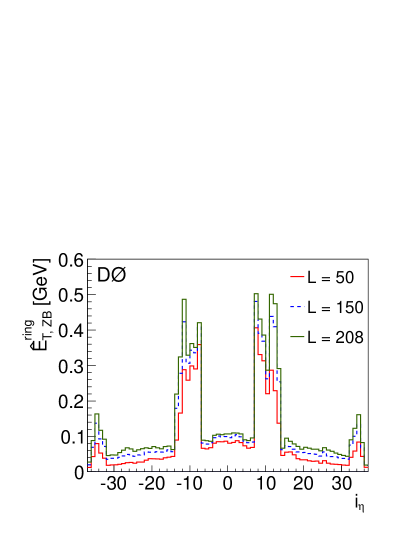
Figure 3: (color online) Average transverse energy per $i_{\eta}$ ring in ZB events selected as discussed in the text. Lines with various colors correspond to ${\mathcal{L}}={50,150\text{ and }208\mskip 4.0mu plus 2.0mu minus 2.5mu\textnormal{$\!\times 10^{30}\,\textnormal{cm}^{-2}\textnormal{s}^{-1}$}}$.

7.2.2 Multiple interactions

The average energy per $i_{\eta}$ ring due to multiple interactions is estimated from the average energy per ring measured in MB events. Figure 4 shows the average transverse energy per $i_{\eta}$ ring $\hat{E}^{\textnormal{ring}}_{\textnormal{T,MB}}$, for MB events with different ${n_{\textnormal{PV}}}$, and corresponding to ${\mathcal{L}}={200\mskip 4.0mu plus 2.0mu minus 2.5mu\textnormal{$\!\times 10^{30}\,\textnormal{cm}^{-2}\textnormal{s}^{-1}$}}$.

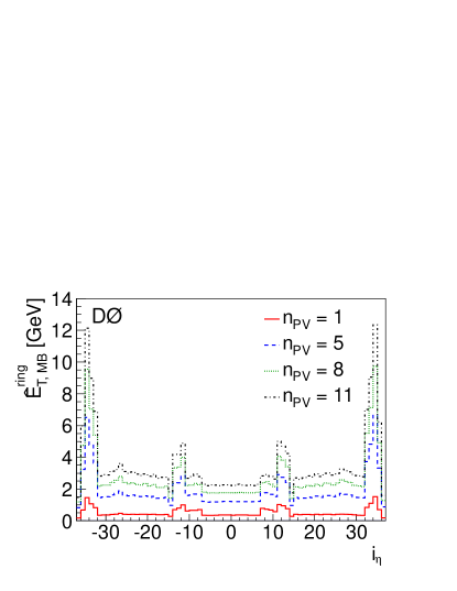
Figure 4: (color online) Average transversed energy in minimum bias events as a function of $i_{\eta}$. Lines with various colors correspond to ${n_{\textnormal{PV}}}=1$, ${n_{\textnormal{PV}}}=5$, ${n_{\textnormal{PV}}}=8$, and ${n_{\textnormal{PV}}}=11$.

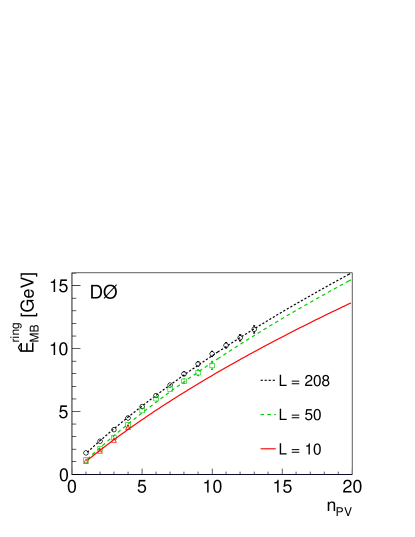
Figure 5: (color online) Minimum bias energy as a function of ${n_{\textnormal{PV}}}$ for one particular ring ${i_{\eta}}=20$. Lines correspond to different luminosities ${\mathcal{L}}={10,50\text{ and }208\mskip 4.0mu plus 2.0mu minus 2.5mu\textnormal{$\!\times 10^{30}\,\textnormal{cm}^{-2}\textnormal{s}^{-1}$}}$.

For each $i_{\eta}$ and $\mathcal{L}$ bin, the average MB energy is measured as a function of $n_{\textnormal{PV}}$, for ${n_{\textnormal{PV}}}\leq 14$, and extrapolated up to ${n_{\textnormal{PV}}}\leq 20$ using function:

$$\hat{E}^{\textnormal{ring}}_{\textnormal{MB}}{({n_{\textnormal{PV}}})}=(a+b\,\sqrt{1+4c\,{n_{\textnormal{PV}}}}-1)/2c,$$ (25)

with empirically determined constants $a$, $b$, and $c$. The form of the function assumes that the offset energy depends on the number of $p\bar{p}$ collision, $n_{\textnormal{PV\,true}}$, linearly as $a+b\,{n_{\textnormal{PV\,true}}}$, while the observed number of primary vertices is ${n_{\textnormal{PV}}}={n_{\textnormal{PV\,true}}}+c\,{n_{\textnormal{PV\,true}}^{2}}$, due to fake tracks and vertices [26]. Figure 5 illustrates the average offset energy for MB events, $\hat{E}^{\textnormal{ring}}_{\textnormal{MB}}$, as a function of ${n_{\textnormal{PV}}}$ for ${i_{\eta}}=20$ (taken as an example) collected at different luminosities. This simple model accurately describes the observed dependency of the minimum bias energy on $n_{\textnormal{PV}}$.

We define the average energy per $i_{\eta}$ ring due to multiple interactions as the difference between the MB energy $\hat{E}_{\textnormal{MB}}^{\textnormal{ring}}$ for events with ${n_{\textnormal{PV}}}$ $p\bar{p}$ collision vertices and with exactly one $p\bar{p}$ collision vertex:

$$\hat{E}_{\textnormal{MI}}^{\textnormal{ring}}({i_{\eta}},{n_{\textnormal{PV}}},{\mathcal{L}})\\ =\hat{E}_{\textnormal{MB}}^{\textnormal{ring}}({i_{\eta}},{n_{\textnormal{PV}}},{\mathcal{L}})-\hat{E}_{\textnormal{MB}}^{\textnormal{ring}}({i_{\eta}},{n_{\textnormal{PV}}}=1,{\mathcal{L}}).$$ (26)

7.2.3 Total offset energy

The estimated total offset energy for a jet, $\hat{E}_{\textnormal{O}}$, is calculated using the average energy for each ring ($\hat{E}_{\textnormal{O}}^{\textnormal{ring}}$), taking into account the fraction of towers ($f^{\textnormal{twr}}$) in each $i_{\eta}$ ring within the jet cone:

$$\hat{E}_{\textnormal{O}}({\eta_{\textnormal{det}}^{\textnormal{}}},{n_{\textnormal{PV}}},{\mathcal{L}})=\sum_{{i_{\eta}}\in{\mathcal{R}_{\textnormal{cone}}}}\hat{E}_{\textnormal{O}}^{\textnormal{ring}}({{i_{\eta}},{n_{\textnormal{PV}}},{\mathcal{L}}})\times\\ \times f^{\textnormal{twr}}({{i_{\eta}},{\eta_{\textnormal{det}}^{\textnormal{}}}}),$$ (27)

where $\eta_{\textnormal{det}}^{\textnormal{}}$ is the detector pseudorapidity of the cone axis.

7.3 Results

Figures 6 and 7 show the estimated jet offset energy as a function of $\eta_{\textnormal{det}}^{\textnormal{}}$ for events with different number of reconstructed $p\bar{p}$ collision vertices. This estimate has been obtained using Eq. 27, separately for jets with ${\mathcal{R}_{\textnormal{cone}}}=0.7$ and 0.5, and ${\mathcal{L}}={80\mskip 4.0mu plus 2.0mu minus 2.5mu\textnormal{$\!\times 10^{30}\,\textnormal{cm}^{-2}\textnormal{s}^{-1}$}}$, which represents the average instantaneous luminosity of the MB sample. The offset energy for ${\mathcal{R}_{\textnormal{cone}}}=0.5$ jets is approximately a factor of two smaller than for ${\mathcal{R}_{\textnormal{cone}}}=0.7$ jets, in agreement with the expectation based on the ratio of their geometrical areas.

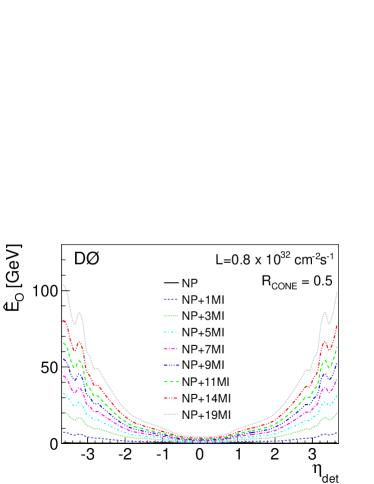
Figure 6: (color online) Estimated total jet offset energy, $\hat{E}_{\textnormal{O}}$, as a function of $\eta_{\textnormal{det}}^{\textnormal{}}$, for jets with ${\mathcal{R}_{\textnormal{cone}}}=0.5$. The different lines show the prediction for noise and pile-up (NP) only (${n_{\textnormal{PV}}}=1$), as well as NP and multiple interactions (MI) (${n_{\textnormal{PV}}}>1$).

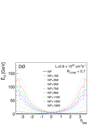
Figure 7: (color online) Same as on Fig. 6 for jets with ${\mathcal{R}_{\textnormal{cone}}}=0.7$.

7.4 Zero-suppression bias correction

The total offset energy estimated from MB and ZB events can differ substantially from the true offset energy inside the jet cone. This is because the calorimeter cells inside the jet cone already contain energy from the hard interaction and therefore they are more likely to be above threshold compared to the cells outside the jet. As a result, the actual offset energy deposited inside the jet cone is higher than that estimated using the MB and ZB events with a lower cell occupancy. We thus derive an average correction factor from the offset-corrected jet energy to the actual jet energy in the absence of noise, pile-up, and multiple interactions. This correction factor can be estimated in MC by comparing the measured jet energy from the same high-${p^{\textnormal{}}_{\textnormal{T}}}$ events processed with and without offset energy added.

The factor which corrects for this effect (${k_{\textnormal{O}}^{\textnormal{ZS}}}$) is estimated comparing the measured energy of the leading jet from the same high-$p^{\textnormal{}}_{\textnormal{T}}$ ${\gamma}+\textnormal{jet}$ event with and without offset energy added, denoted by $E^{\textnormal{meas}}_{\textnormal{}}$ and $E^{\textnormal{meas,noZB}}$, respectively:

$${{k_{\textnormal{O}}^{\textnormal{ZS}}}}=\frac{E^{\textnormal{meas,noZB}}}{{E^{\textnormal{meas}}_{\textnormal{}}}-\hat{E}_{\textnormal{O}}}.$$ (28)

For this purpose, we consider the same ${\gamma}+\textnormal{jet}$ MC events processed in three ways (see Sec. 6.2):

1. no ZB overlay, i.e., no offset energy from noise, pile-up, and multiple interactions. This provides the reference level to which to correct ($E^{\textnormal{meas,noZB}}$).

2. ZB overlay (providing $E^{\textnormal{meas}}_{\textnormal{}}$):

   1. Using zero-suppressed overlay the derived correction factor will be applicable to the jet energy scale calibration in MC since the standard MC simulation uses zero-suppressed ZB overlay,

   2. Using ZB overlay without zero-suppression, the derived correction factor will be applicable to the jet energy scale calibration in data since they provide the most realistic description of the per-cell energy spectrum arising from noise, pileup, and multiple interactions.

Only matched jets contribute to Eq. 28, i.e., only events where a reconstructed jet in the case of ZB overlay is unambiguously matched within $\Delta{\cal R}<{\mathcal{R}_{\textnormal{cone}}}/2$ with a jet in the case of no ZB overlay are considered. Furthermore, we have the same set of physical events (with common partonic origin) in the samples without ZB overlay and with ZB overlay, both suppressed and unsuppressed. The correction is measured separately for jets with ${\mathcal{R}_{\textnormal{cone}}}=0.7$ and 0.5, in intervals of 0.4 of jet $\left|{{\eta_{\textnormal{det}}^{\textnormal{}}}}\right|$, and as a function of $p^{\prime}_{\textnormal{T}}$ (defined in Eq. 15) for suppressed and unsuppressed ZB overlay.

The ${k_{\textnormal{O}}^{\textnormal{ZS}}}$ factor depends on $\eta_{\textnormal{det}}^{\textnormal{}}$ and $n_{\textnormal{PV}}$ and it is extracted for the average number of $p\bar{p}$ collision vertices, $\langle{n_{\textnormal{PV}}}\rangle$. Figure 8 illustrates the extracted ${k_{\textnormal{O}}^{\textnormal{ZS}}}$ factor for two $\eta_{\textnormal{det}}^{\textnormal{}}$ intervals.

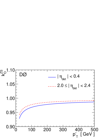
Figure 8: Correction factor for the zero-suppression bias ${k_{\textnormal{O}}^{\textnormal{ZS}}}$ for ${\mathcal{R}_{\textnormal{cone}}}=0.7$ jets in the unsuppressed ZB overlay sample within ${\left|{{\eta_{\textnormal{det}}^{\textnormal{}}}}\right|}<0.4$, and $2.0\leq{\left|{{\eta_{\textnormal{det}}^{\textnormal{}}}}\right|}<2.4$ ($\left<{{n_{\textnormal{PV}}}}\right>=2.6$, Run IIb2 data).

7.5 Uncertainties

The offset correction measurement in data as given by Eq. 27 has a high statistical precision. Statistical uncertainties do not exceed 2%.

The systematic uncertainty originates from the fitting procedure for $\hat{E}_{\textnormal{MB}}^{\textnormal{ring}}$ and is estimated for each $i_{\eta}$ ring (see Fig. 5) from the residual difference between fit and data. The uncertainty is found to be mildly dependent on $\eta_{\textnormal{det}}^{\textnormal{}}$ and varies between $50\text{ and }200\mskip 4.0mu plus 2.0mu minus 2.5mu\textnormal{MeV}$ for ${\mathcal{R}_{\textnormal{cone}}}=0.5$ and between $100\text{ and }350\mskip 4.0mu plus 2.0mu minus 2.5mu\textnormal{MeV}$ for ${\mathcal{R}_{\textnormal{cone}}}=0.7$.

Figure 9 shows the relative systematic uncertainty as a function of the measured transverse momentum of the jet, for jets with ${\mathcal{R}_{\textnormal{cone}}}=0.5$ and $0.7$, and ${\eta_{\textnormal{det}}^{\textnormal{}}}=3.0$, which has the largest systematic uncertainty. The systematic uncertainties of the jet transverse momenta due to the offset correction are typically less than $1\%$.

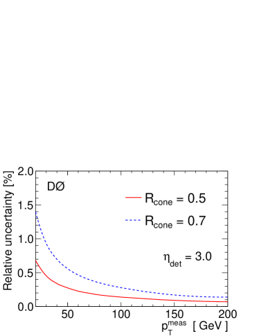
Figure 9: Relative systematic uncertainty on the offset correction as a function of the measured transverse momentum $p^{\textnormal{meas}}_{\textnormal{T}}$ of the jet, for jets with ${\mathcal{R}_{\textnormal{cone}}}=0.5$ and $0.7$, and ${\eta_{\textnormal{det}}^{\textnormal{}}}=3.0$.

8 Absolute MPF response

This section describes the determination of the response correction for central calorimeter jets using the MPF method as described in Sec. 5. The response from the central region provides the main correction factor for jet energy calibration. The calibration of forward jets, relative to the response in the central region, is described in Sec. 9.

8.1 Sample selection

The ${\gamma}+\textnormal{jet}$ samples described in Sec. 6 are used for the determination of the absolute response correction in both data and MC. Further selection criteria are applied to extract a subset of events with suitable characteristics for the measurement of the jet response via the MPF method. These requirements are:

• Events are rejected unless they have exactly one or two reconstructed $p\bar{p}$ collision vertices. The main vertex associated with the hard interaction must satisfy the vertex selection criteria discussed in Sec. 3.1. The inclusion of events with two vertices doubles the size of the sample and has been shown not to introduce any bias.

• Each event must have exactly one photon candidate with measured transverse momentum, ${p^{\textnormal{meas}}_{\textnormal{T{$\gamma$}}}}>{7\mskip 4.0mu plus 2.0mu minus 2.5mu\textnormal{$\textnormal{GeV}$}}$, satisfying the tight photon identification criteria (see Sec. 3.3). The photons must be in the central calorimeter corresponding to $\left|{{\eta_{\textnormal{det}}^{\textnormal{{$\gamma$}}}}}\right|<1$. The momentum $p^{\textnormal{meas}}_{\textnormal{T{$\gamma$}}}$ does not include the photon calibration described in Sec. 8.3.1.

• To avoid a possible bias caused by trigger inefficiency, $p^{\textnormal{meas}}_{\textnormal{T{$\gamma$}}}$ is required to be in the high efficiency range of the particular trigger used to collect the event. In addition, the directions of the photon candidate and the electromagnetic trigger tower at Level 1 trigger must match within ${\Delta\mathcal{R}}<0.4$.

• Each event has to have exactly one reconstructed jet (with ${\mathcal{R}_{\textnormal{cone}}}=0.7$ or 0.5, as appropriate) satisfying the jet selection criteria described in Sec. 3.4. This jet is referred to as the “probe jet”. No additional jet is allowed in the event, except if its direction matches the photon candidate within ${\Delta\mathcal{R}}<0.2$, since the photon candidate can also be reconstructed as a jet.

• The probe jet must have ${\left|{{\eta_{\textnormal{det}}^{\textnormal{}}}}\right|}<0.4$, so that its core is well contained inside the central calorimeter.

• The photon and jet are required to be back-to-back in the $r$-$\phi$ plane: the difference of their azimuthal angle should be $\Delta{\phi}({\gamma},\textnormal{jet})>3.0$ rad.

• Data events with cosmic muon candidates, indentified using muon system timing information, are rejected.

• To further eliminate cosmic rays and other physics backgrounds, an upper limit is imposed on the ratio ${{\not\!\!{E^{\textnormal{}}_{\textnormal{T}}}}}/{p^{\textnormal{meas}}_{\textnormal{T{$\gamma$}}}}$ in the range of 0.65 to 1.1, where a looser cut corresponds to the lower photon $p^{\textnormal{}}_{\textnormal{T}}$ [11, 38].

8.2 Backgrounds in the ${\gamma}+\textnormal{jet}$ sample

Two types of background contaminate the ${\gamma}+\textnormal{jet}$ sample: events with electrons or multiple photons from electroweak interactions that are misidentified as a single photon, and events where strong interactions produce a jet misidentified as photon.

Background processes of the first type are $W(\to e\nu)+\textnormal{jet}$, $Z/{\gamma}^{*}(\to{{e^{+}e^{-}}})+\textnormal{jet}$, and diphoton production. The contributions from these backgrounds are estimated from MC simulation. In the case of $W(\to e\nu)+\textnormal{jet}$ events, with the electron misidentified as a photon, the neutrino will contribute additional missing transverse energy ${\not\!\!{E^{\textnormal{}}_{\textnormal{T}}}}$. The combination of the track veto (part of the photon identification criteria) and the capping of the ratio ${{\not\!\!{E^{\textnormal{}}_{\textnormal{T}}}}}/{p^{\textnormal{meas}}_{\textnormal{T{$\gamma$}}}}$ reduces the contribution from these processes to a negligible level, less than $0.5\%$. Contributions from $Z+\textnormal{jet}$ and diphoton events are found to be even smaller. The total expected bias on the MPF response is studied in MC and is estimated to be below $0.1\%$.

The second type of background is represented by dijet events, where one of the partons showers to produce a well isolated, energetic $\pi^{0}$ or $\eta$ meson, decaying into a multi-photon final state. The probability for a jet to be misidentified as a photon depends on the photon identification criteria but is typically very small. Nevertheless this background contamination remains sizable, particularly for photons with low transverse momentum $p^{\textnormal{}}_{\textnormal{T{$\gamma$}}}$, due to the high rate of dijet production.

The photon purity is estimated using the ${\gamma}+\textnormal{jet}$ and dijet ($\gamma$-like) MC samples described in Sec. 6.2. To estimate background from the dijet events remaining after the photon selection, we use the scalar sum of the transverse momenta of all tracks in a hollow cone of $0.05<{\Delta\mathcal{R}}<0.7$ around the direction of the photon candidate (see Sec. 3.3). The distributions for the simulated photon signal and dijet background samples are fitted to the data for each ${p^{\textnormal{meas}}_{\textnormal{T{$\gamma$}}}}$ bin using a maximum likelihood fit [39] to obtain the fractions of signal and background components in the data. The systematic uncertainties on the purity measurement are estimated from the uncertainties on the fit result and from a comparison with alternative fitting functions. An additional contribution is included due to the dependencies on the fragmentation model implemented in pythia. The overall systematic uncertainty is found to be $5\%$ at ${p^{\textnormal{}}_{\textnormal{T{$\gamma$}}}}\approx{30\mskip 4.0mu plus 2.0mu minus 2.5mu\textnormal{$\textnormal{GeV}$}}$, $3\%$ at ${p^{\textnormal{meas}}_{\textnormal{T{$\gamma$}}}}\approx{50\mskip 4.0mu plus 2.0mu minus 2.5mu\textnormal{$\textnormal{GeV}$}}$, and $2\%$ at ${p^{\textnormal{meas}}_{\textnormal{T{$\gamma$}}}}\gtrsim{70\mskip 4.0mu plus 2.0mu minus 2.5mu\textnormal{$\textnormal{GeV}$}}$ [34].

Figure 10 illustrates the estimated purity of the selected ${\gamma}+\textnormal{jet}$ sample with central jets (${\left|{{\eta_{\textnormal{det}}^{\textnormal{}}}}\right|}<0.4$, as an example) as a function of $E^{\prime}$ (defined in Eq. 14). Individual points represent purity determined from the data. The purity improves for higher $E^{\prime}$, as the probability for production of isolated EM showers through the fragmentation process decreases.

The presence of this instrumental background leads to a positive bias in the measured MPF response, since the photon candidate is usually surrounded by hadronic activity resulting from the fragmentation of the original parton. This effect can be suppressed by using more stringent photon identification criteria, but it cannot be completely eliminated. Therefore, we explicitly correct the measured MPF response for this effect.

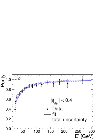
Figure 10: Photon purity measured in the ${\gamma}+\textnormal{jet}$ data sample selected using tight photon identification criteria, for ${\left|{{\eta_{\textnormal{det}}^{\textnormal{}}}}\right|}<0.4$ as a function of $E^{\prime}$. Also shown is the total uncertainty band.

8.3 Method

The measurement of the absolute MPF response is discussed in Sec. 5.1.2. The goal is to estimate the MPF response for $\gamma$+jet events with the photon at the particle level. In the case of MC, this is achieved by using a modified version of Eq. 13:

$${R_{\textnormal{MPF,CC}}^{\textnormal{{${\gamma}+\textnormal{jet}$}}}}=1+\frac{{{\not\!\!\vec{E}}^{\textnormal{}}_{\textnormal{T}}}\cdot\vec{n}_{\textnormal{T{$\gamma$}}}}{{p^{\textnormal{ptcl}}_{\textnormal{T{$\gamma$}}}}},$$ (29)

where, on an event-by-event basis, the particle level photon transverse momentum, $\vec{p}^{\textnormal{ ptcl}}_{\textnormal{T{$\gamma$}}}$, is used for the tag, and ${\not\!\!\vec{E}}^{\textnormal{}}_{\textnormal{T}}$ is corrected accordingly, similarly to Eq. 2:

$${{\not\!\!\vec{E}}^{\textnormal{}}_{\textnormal{T}}}\enskip\Rightarrow\enskip{{\not\!\!\vec{E}}^{\textnormal{}}_{\textnormal{T}}}+{\vec{p}^{\textnormal{ }}_{\textnormal{T{$\gamma$}}}}-{\vec{p}^{\textnormal{ ptcl}}_{\textnormal{T{$\gamma$}}}}.$$ (30)

In the case of data, as discussed in Sec. 5.2, the application of Eq. 13 results in a measurement of the MPF response which is affected by the bias in measured photon transverse momentum, as well as the presence of the dijet background. Explicit corrections for these biases are discussed below.

8.3.1 Photon energy scale correction

The first correction is related to the calibration of the photon energy scale. As discussed in Sec. 2.3, the absolute energy calibration of the electromagnetic calorimeter is obtained using electrons from $Z\to{e^{+}e^{-}}$ decays with about 0.5% accuracy. Corrections for the energy loss of electrons in the material in front of the calorimeter as a function of $\eta_{\textnormal{det}}^{\textnormal{}}$ and $p^{\textnormal{}}_{\textnormal{T}}$ are determined in MC and applied to electromagnetic objects in data. However, photons interact less with the material of the detector than electrons, and as a result the electron energy scale correction overcorrects the photon energy ($E^{\textnormal{meas}}_{\textnormal{{$\gamma$}}}$) relative to the particle level ($E^{\textnormal{ptcl}}_{\textnormal{{$\gamma$}}}$). This effect is particularly sizable at low energy.

The difference in the response of the calorimeter for electrons and photons is evaluated in dedicated MC with an improved geant description of electromagnetic showers [24], which is not used for standard simulation of physics processes due to its low execution speed. Calorimeter response is simulated for single photons and electrons entering the D0 detector at different angles and positions. At low energies (${E^{\textnormal{meas}}_{\textnormal{{$\gamma$}}}}\approx{20\mskip 4.0mu plus 2.0mu minus 2.5mu\textnormal{GeV}}$), the photon energy overcorrection (Fig. 11) is estimated to be about $3\%$. The difference between electrons and photons becomes smaller, but still remains sizable, at high energies. This photon energy scale correction is applied to the reconstructed EM object, and the missing energy is corrected accordingly (see Eq. 30).

Three main sources of photon energy scale systematic uncertainties are considered: the electron energy calibration, the difference between photon and electron energy scale, and the contamination by $\gamma$-like jets. The first is estimated to be about $0.5\%$ and it is mostly connected with long-term stability of the calorimeter response. The second is due to the different nature of photon and electron interactions with the material in front of the calorimeter. This effect is estimated by varying the amount of this material in the simulation within its uncertainty. Finally, the energy calibration of the candidate photons is affected by the presence of misidentified $\gamma$-like jets. The size of this effect is found to be smaller than $0.2\%$, and included in the uncertainty.

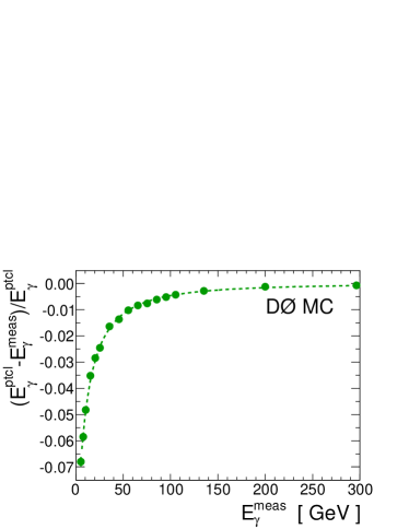
Figure 11: Photon energy scale correction as estimated from dedicated MC. This correction is applied to photons after the calibration of the EM calorimeter described in Sec. 2.3.

8.3.2 Background correction

The ${\gamma}+\textnormal{jet}$ sample selected according to criteria of Sec. 3 is a mixture of ${\gamma}+\textnormal{jet}$ signal events and dijet background. The photon candidate in the latter sample is caused by $\gamma$-like jets. The measured MPF response for this mixed sample can be expressed as a linear combination of the MPF responses for signal and background weighted by the respective sample fractions:

$${R_{\textnormal{MPF,$\eta$}}^{\textnormal{mixture}}}=\rho_{\eta}{R_{\textnormal{MPF,$\eta$}}^{\textnormal{{${\gamma}+\textnormal{jet}$}}}}+(1-\rho_{\eta}){R_{\textnormal{MPF,$\eta$}}^{\textnormal{{$\textnormal{dijet}$}}}},$$ (31)

where both MPF responses are with respect to the photon $p^{\textnormal{}}_{\textnormal{T}}$, and $\rho_{\eta}$ is the ${\gamma}+\textnormal{jet}$ sample purity (see, e.g., Fig. 10), as function of the jet pseudorapidity $\eta_{\textnormal{det}}^{\textnormal{}}$. Since the same approach is used later for the relative calibration of forward jets, the dependence on jet $\eta_{\textnormal{det}}^{\textnormal{}}$ is explicitly kept in this formula. The relative difference between the MPF response of the mixed sample and the MPF response of the pure sample is then:

$$c_{\textnormal{bckg},\eta}\equiv\frac{{R_{\textnormal{MPF,$\eta$}}^{\textnormal{mixture}}}}{{R_{\textnormal{MPF,$\eta$}}^{\textnormal{{${\gamma}+\textnormal{jet}$}}}}}-1=(1-\rho_{\eta})\left(\frac{{R_{\textnormal{MPF,$\eta$}}^{\textnormal{{$\textnormal{dijet}$}}}}}{{R_{\textnormal{MPF,$\eta$}}^{\textnormal{{${\gamma}+\textnormal{jet}$}}}}}-1\right),$$ (32)

and the correction factor $k_{\textnormal{R}}^{\textnormal{{$\gamma$}}}$ described in Eq. 17 can therefore be written as

$${k_{\textnormal{R}}^{\textnormal{{$\gamma$}}}}=\frac{1}{1+c_{\textnormal{bckg},\eta}},$$ (33)

where $\eta$ refers to the pseudorapidity of the jet recoiling from the central EM object.

Jet response in a pure ${\gamma}+\textnormal{jet}$ sample and in dijet background is estimated from MC. The response from MC does not accurately reproduce the jet response in the data. Therefore the background correction is determined with the corrected MC simulation of Sec. 14. Figure 12 compares $R_{\textnormal{MPF,CC}}^{\textnormal{{$\textnormal{dijet}$}}}$, defined similarly to Eq. 29 (with a photon candidate energy corrected according to Fig. 11), and $R_{\textnormal{MPF,CC}}^{\textnormal{{${\gamma}+\textnormal{jet}$}}}$ as predicted by the MC, for events with a jet within ${\left|{{\eta_{\textnormal{det}}^{\textnormal{}}}}\right|}<0.4$.

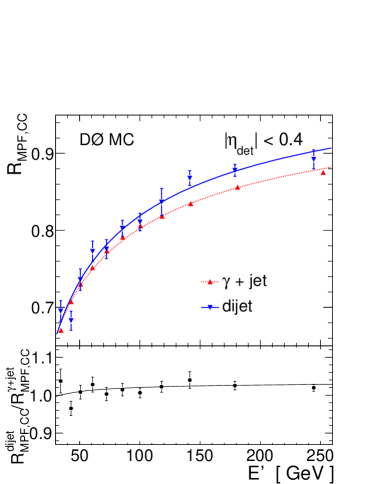
Figure 12: Comparison of MPF responses in ${\gamma}+\textnormal{jet}$ and dijet MC samples selected as described in Sec. 8.1 in the events with central jets. The lines in the upper panel show fits to the responses in the ${\gamma}+\textnormal{jet}$ and dijet events, respectively. The line in the bottom plot shows a ratio of fits of those responses, while points correspond to the ratio ${R_{\textnormal{MPF,CC}}^{\textnormal{{$\textnormal{dijet}$}}}}/{R_{\textnormal{MPF,CC}}^{\textnormal{{${\gamma}+\textnormal{jet}$}}}}$ in each bin.

The ratio of fits of responses in the ${\gamma}+\textnormal{jet}$ and dijet events appearing in the right side of Eq. 32, also shown in Fig. 12, is $1\%-3\%$ above unity, due to additional hadronic activity around the misidentified photon in the dijet sample. This activity reduces ${\not\!\!{E^{\textnormal{}}_{\textnormal{T}}}}$ in the direction of the jet, increasing the measured MPF response relative to that for the ${\gamma}+\textnormal{jet}$ sample. The tight photon criteria, which are applied for the final jet response measurements, suppress much of this additional hadronic activity, yielding a MPF response for the dijet sample which is not more than 2% larger than for the ${\gamma}+\textnormal{jet}$ sample.

8.4 Results

The MPF response as a function of $E^{\prime}$ for ${\mathcal{R}_{\textnormal{cone}}}=0.7$ jets is shown in Fig. 13 for MC and data. In the case of MC, the MPF response is obtained directly using Eq. 29. In the case of data, the MPF response for the mixture sample is first computed using Eq. 13 and then corrected using the following equation,

$${R_{\textnormal{MPF,CC}}^{\textnormal{{${\gamma}+\textnormal{jet}$}}}}={R_{\textnormal{MPF,CC}}^{\textnormal{mixture}}}\,{k_{\textnormal{R}}^{\textnormal{{$\gamma$}}}},$$ (34)

where $k_{\textnormal{R}}^{\textnormal{{$\gamma$}}}$ is defined in Eq. 33.

In both data and MC, the tight photon identification criteria are used. Since jet energies do not enter directly into the calculation of the MPF response, the dependence on ${\mathcal{R}_{\textnormal{cone}}}$ is expected to be very small. As an example, the MPF response for ${\mathcal{R}_{\textnormal{cone}}}=0.5$ is about $0.5\%$ higher at ${E^{\prime}}\approx{100\mskip 4.0mu plus 2.0mu minus 2.5mu\textnormal{GeV}}$ than for ${\mathcal{R}_{\textnormal{cone}}}=0.7$, in both data and MC. The measured MPF response is fitted using the parameterization in Eq. 16.

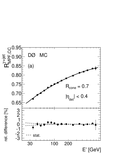
(a)

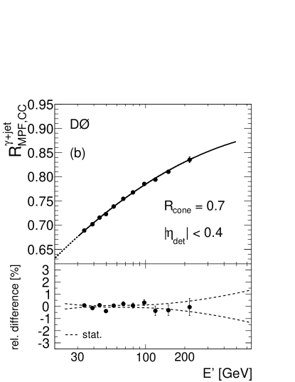
(b)

Figure 13: Absolute MPF response for ${\mathcal{R}_{\textnormal{cone}}}=0.7$ jets in LABEL:sub@f_rjet7_MC MC and LABEL:sub@f_rjet7_data data as a function of $E^{\prime}$. The solid line indicates the fit to the function in Eq. 16. The lower plots show the relative difference of the points with respect to the fitted function, along with the statistical uncertainty from the fit.

8.5 Uncertainties

In the case of the MPF response measurement in MC, the only uncertainty is from the statistical uncertainty of the fit (including the full covariance matrix) shown in 13a. The main sources of uncertainty in the MPF response measurement in data are shown in Fig. 14 for ${\mathcal{R}_{\textnormal{cone}}}=0.7$ jets. They include the statistical uncertainty of the fit, the uncertainties on the photon energy scale, on the correction for the dijet background contamination, on the high energy extrapolation procedure (see below), and an uncertainty to account for the stability of response versus time. The uncertainties for ${\mathcal{R}_{\textnormal{cone}}}=0.5$ jets are almost identical except the statistical uncertainty and those connected with the high energy extrapolation procedure which is performed only for ${\mathcal{R}_{\textnormal{cone}}}=0.7$ jets.

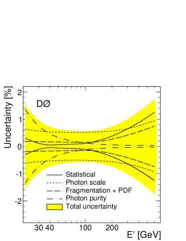
Figure 14: (color online) Relative uncertainties on the MPF response measurement in data for ${\mathcal{R}_{\textnormal{cone}}}=0.7$ jets. The shaded region shows the total uncertainty, while the statistical uncertainty is shown by the solid line. Uncertainties related to photon energy scale and purity, parton-to-hadron fragmentation and PDF effects are also shown. Uncertainties for ${\mathcal{R}_{\textnormal{cone}}}=0.5$ jets are very similar.

The main source of uncertainty in data is the photon energy scale in almost the entire range of accessible energies. At low jet energies (below $30\mskip 4.0mu plus 2.0mu minus 2.5mu\textnormal{GeV}$), the uncertainty due to the dijet background correction dominates.

The uncertainty on the dijet background correction is related to the uncertainty on $c_{\textnormal{bckg}}$ (Eq. 32), with two independent components: purity and relative response between ${\gamma}+\textnormal{jet}$ and dijet MC events. Ideally, the corrected MPF response in data should be independent of the photon identification criteria, despite differences in purity. We have compared the MPF response in data for the different photon criteria, before and after the background correction. The observed small residual differences after background correction are consistent with the assigned systematic uncertainty. Part of the observed difference between medium and tight criteria is unrelated to the background and can already be observed in ${\gamma}+\textnormal{jet}$ MC with the photon at the particle level. This effect is believed to be caused by distortions in the hadronic activity in the photon hemisphere, which propagates to ${\not\!\!{E^{\textnormal{}}_{\textnormal{T}}}}$, as a result of tightening the photon isolation. This effect will be corrected by the topology bias correction (see Sec. 10.2), and therefore it does not represent an additional source of systematic uncertainty. The dijet background correction (see Eq. 33) can be verified using data. Jet responses with different photon selections should be equal once they are corrected for the background admixture. To cover potential mismodeling in the MC simulation, an additional $1\%$ systematic uncertainty is assigned to the relative difference between the response in the ${\gamma}+\textnormal{jet}$ and background dijet samples. This is roughly half the size of the background correction in case of the tight photon selection (Fig. 12).

Measurements from events with only two or three jets, typically using jets with ${\mathcal{R}_{\textnormal{cone}}}=0.7$, include jets with very large energy (up to $1\mskip 4.0mu plus 2.0mu minus 2.5mu\textnormal{TeV}$). The MC is used to constrain the response for such high energy jets in data. The uncertainty on this high energy extrapolation includes the following two sources of systematic uncertainty: parton distribution functions (PDFs) and fragmentation model. These uncertainties are related to the dependence of the predicted hadron spectra at high energy on the parton flavor of jets as well as the modeling of the fragmentation. More details about the high energy extrapolation can be found in Ref. [4].

9 Relative MPF response

In the previous section we derived the absolute response for jets in the very central part of the calorimeter. The relative MPF response normalizes the response for jet energy as a function of pseudorapidity, allowing the description of the response for jets in any part of the detector. The derivation of this correction relies on events from two different processes, ${\gamma}+\textnormal{jet}$ and dijet production (see Sec. 5.1.3).

The selection criteria for ${\gamma}+\textnormal{jet}$ events are identical to those used for the measurement of absolute response (Sec. 8.1), with the exception that the probe jet is not restricted to the central calorimeter. The samples used for the determination of the dijet correction in MC are described in Sec. 6.2.

The selection of dijet events closely follows that of ${\gamma}+\textnormal{jet}$ events, with one of the jets playing the role of the photon. Events with no reconstructed PV or with more than four PVs are rejected. Events must have exactly two reconstructed jets with ${\mathcal{R}_{\textnormal{cone}}}=0.7$ or $0.5$ as appropriate, satisfying the jet selection criteria described in Sec. 3.4. Events with additional reconstructed jets that do not satisfy those criteria are rejected. At least one of the jets must be within ${\left|{{\eta_{\textnormal{det}}^{\textnormal{}}}}\right|}\leq 0.4$, so that its core is well contained inside the central calorimeter. This jet is referred to as the “tag” whereas the other jet is referred to as the “probe”. If both jets have ${\left|{{\eta_{\textnormal{det}}^{\textnormal{}}}}\right|}<0.4$ both possibilities for tag and probe assignments are considered. To avoid a bias from the trigger, the uncorrected transverse momentum of the tag jet is required to be large enough so that the efficiency of the trigger for such jets is above $98\%$. The jets are required to be back-to-back in the ${r}$-${\phi}$ plane, i.e., the difference of their azimuthal angles, $\Delta{\phi}\left(\textnormal{probe},\textnormal{tag}\right)$, must be larger than $3.0\mskip 4.0mu plus 2.0mu minus 2.5mu\textnormal{rad}$. Events with muons that are cosmic ray candidates are rejected. To further reduce cosmic rays, the ratio of the measured ${\not\!\!{E^{\textnormal{}}_{\textnormal{T}}}}$ over the $p^{\textnormal{}}_{\textnormal{T}}$ of the most energetic jet is required to be ${{\not\!\!{E^{\textnormal{}}_{\textnormal{T}}}}}/{p^{\textnormal{}}_{\textnormal{T}}}<0.7$.

9.1 Method

The relative response correction, $F_{\eta}^{\textnormal{}}$, is evaluated for jets up to ${\left|{{\eta_{\textnormal{det}}^{\textnormal{}}}}\right|}\leq 3.6$. The samples are split according to the pseudorapidity of the probe jet, each group typically spanning $\Delta{\eta_{\textnormal{det}}^{\textnormal{}}}=0.1$, with the exception that the range is narrower (0.05) for the ICD region, where the response varies rapidly with $\eta_{\textnormal{det}}^{\textnormal{}}$, and wider (up to 0.4) starting with ${\left|{{\eta_{\textnormal{det}}^{\textnormal{}}}}\right|}>2.0$ in order to compensate for decreased statistics.

Although similar in spirit, the treatment of ${\gamma}+\textnormal{jet}$ and dijet events differs in some details due to the different nature of the samples. The following sections describe their treatment separately.

9.1.1 Relative response in the ${\gamma}+\textnormal{jet}$ sample

The MPF response $R_{\textnormal{MPF,$\eta$}}^{\textnormal{}}$ (see Eq. 12) is estimated as the average over all the events in each $E^{\prime}$ bin, similar to the procedure described in Sec. 8.3, in each ${\eta_{\textnormal{det}}^{\textnormal{}}}$ region independently. In the case of data, the estimated response does not correspond exactly to the ${\gamma}+\textnormal{jet}$ response because of the contamination by dijet events and the imperfect calibration of the photon energy, as discussed in Sec. 8.3. In the case of MC, the measured MPF response for a pure ${\gamma}+\textnormal{jet}$ sample is known at the particle level directly from the MC information. This response is denoted as $R_{\textnormal{MPF,$\eta$}}^{\textnormal{{${\gamma}+\textnormal{jet}$}}}$.

The relative MPF response correction is computed as:

$${F_{\eta}^{\textnormal{{${\gamma}+\textnormal{jet}$}}}}=\frac{{R_{\textnormal{MPF,$\eta$}}^{\textnormal{{${\gamma}+\textnormal{jet}$}}}}\left({E^{\prime}}\right)}{{R_{\textnormal{MPF,CC}}^{\textnormal{{${\gamma}+\textnormal{jet}$}}}}\left({E^{\prime}}\right)}.$$ (35)

The denominator, measured in Sec. 8.4, represents the MPF response of a jet with approximately the same energy as the probe, but measured in the central calorimeter.

Figure 15 shows the $F_{\eta}^{\textnormal{{${\gamma}+\textnormal{jet}$}}}$ values measured from ${\gamma}+\textnormal{jet}$ events as a function of $E^{\prime}$ in two different ${\eta_{\textnormal{det}}^{\textnormal{}}}$ regions. The measured $F_{\eta}^{\textnormal{{${\gamma}+\textnormal{jet}$}}}$ differs from Eq. 35 only in that it is not corrected for background contamination (Sec. 8.3.2), for the reason that will be explained in Sec. 9.1.4.

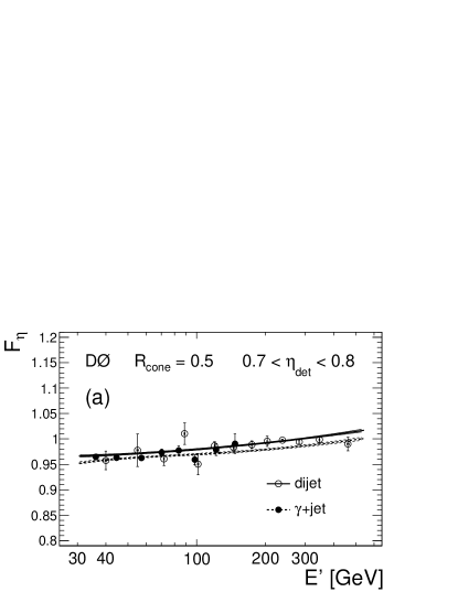
(a)

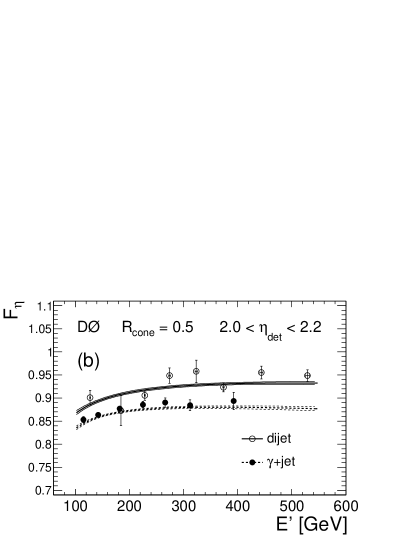
(b)

Figure 15: Relative MPF response for ${\mathcal{R}_{\textnormal{cone}}}=0.5$ jets in data as a function of $E^{\prime}$ for jets with LABEL:sub@example_feta_central $0.7<{\eta_{\textnormal{det}}^{\textnormal{}}}<0.8$ and LABEL:sub@example_feta_forward $2.0<{\eta_{\textnormal{det}}^{\textnormal{}}}<2.2$ (note the different $E^{\prime}$ scale), measured in the ${\gamma}+\textnormal{jet}$ and dijet samples. The curves represent the result from the global fit discussed in Sec. 9.1.4 with statistical uncertainty shown by the error bands.

9.1.2 Relative response in the dijet sample

The procedure to extract the relative response $F_{\eta}^{\textnormal{}}$ from the dijet sample is complicated by the presence of an uncalibrated jet as the reference object. For a dijet event, we measure the MPF response of a probe jet located at ${\eta_{\textnormal{det}}^{\textnormal{}}}$ relative to the response of the central tag jet ($\left|{{\eta_{\textnormal{det}}^{\textnormal{tag}}}}\right|<0.4$), following Eq. 13, as:

$$R_{\textnormal{relMPF},\eta}^{\textnormal{{$\textnormal{dijet}$}}}=1+\frac{{{\not\!\!\vec{E}}^{\textnormal{}}_{\textnormal{T}}}\cdot\vec{n}^{\textnormal{tag}}_{\textnormal{T}}}{{p^{\textnormal{tag}}_{\textnormal{T}}}},$$ (36)

where $\vec{p}^{\textnormal{ tag}}_{\textnormal{T}}$ is the measured transverse momentum of the tag jet, corrected only for offset energy subtraction. This observable can also be interpreted according to Eq. 12 as:

$$R_{\textnormal{relMPF},\eta}^{\textnormal{{$\textnormal{dijet}$}}}\simeq\frac{{R_{\textnormal{MPF,$\eta$}}^{\textnormal{{$\textnormal{dijet}$}}}}\left({E^{\prime}}\right)}{{R_{\textnormal{MPF,CC}}^{\textnormal{{$\textnormal{dijet}$}}}}\left({p^{\prime}_{\textnormal{T}}}\right)},$$ (37)

where $R_{\textnormal{MPF,$\eta$}}^{\textnormal{{$\textnormal{dijet}$}}}$ $\left({E^{\prime}}\right)$ and $R_{\textnormal{MPF,CC}}^{\textnormal{{$\textnormal{dijet}$}}}$ $\left({p^{\prime}_{\textnormal{T}}}\right)$ denote the MPF response of the probe and tag jets, respectively. The transverse momentum of the tag jet $p^{\textnormal{tag}}_{\textnormal{T}}$, the response $R_{\textnormal{relMPF},\eta}^{\textnormal{{$\textnormal{dijet}$}}}$, and also $E^{\prime}$ and $p^{\prime}_{\textnormal{T}}$, are corrected for the jet resolution bias (Sec. 5.1.1).

$F_{\eta}^{\textnormal{{$\textnormal{dijet}$}}}$ is defined similarly to Eq. 35 for the ${\gamma}+\textnormal{jet}$ events:

$${F_{\eta}^{\textnormal{{$\textnormal{dijet}$}}}}=\frac{R_{\textnormal{relMPF},\eta}^{\textnormal{{$\textnormal{dijet}$}}}\>{R_{\textnormal{MPF,CC}}^{\textnormal{{${\gamma}+\textnormal{jet}$}}}}\left({p^{\prime}_{\textnormal{T}}}\right)}{{R_{\textnormal{MPF,CC}}^{\textnormal{{${\gamma}+\textnormal{jet}$}}}}\left({E^{\prime}}\right)}\cdot r_{{E^{\prime}}},$$ (38)

where the response of the probe jet in the numerator is compared to the response of the tag jet in the denominator. If the dijet responses were used consistently in the $F_{\eta}^{\textnormal{{$\textnormal{dijet}$}}}$ definition, its average in the ${\left|{{\eta_{\textnormal{det}}^{\textnormal{}}}}\right|}\leq 0.4$ region would be unity by construction. Since we do not measure the absolute response from dijet events, the calibration of the tag jet is instead based on the ${\gamma}+\textnormal{jet}$ response, $R_{\textnormal{MPF,CC}}^{\textnormal{{${\gamma}+\textnormal{jet}$}}}$. The factor $r_{{E^{\prime}}}$ corrects for the difference between the two types of response in ${\gamma}+\textnormal{jet}$ and dijet events. It is evaluated by enforcing $F_{\eta}^{\textnormal{{$\textnormal{dijet}$}}}$ to be on average unity for the central region ${\left|{{\eta_{\textnormal{det}}^{\textnormal{}}}}\right|}\leq 0.4$, thus ensuring $F_{\eta\approx 0}^{\textnormal{{$\textnormal{dijet}$}}}\approx 1$. The deviation of the factor $r_{{E^{\prime}}}$ from unity is found to be always smaller than $0.5\%$. Figure 15 shows the measured $F_{\eta}^{\textnormal{{$\textnormal{dijet}$}}}$ (Eq. 38) as a function of $E^{\prime}$ in two different ${\eta_{\textnormal{det}}^{\textnormal{}}}$ regions.

9.1.3 Sample dependence of the relative MPF response

The measured correction $F_{\eta}^{\textnormal{}}$ is significantly different for the ${\gamma}+\textnormal{jet}$ and dijet samples at large pseudorapidities, as illustrated in 15b. The main contribution to the discrepancy, particularly for large ${\eta_{\textnormal{det}}^{\textnormal{}}}$, is from the different parton flavor composition of the ${\gamma}+\textnormal{jet}$ and dijet samples. Whereas the leading jet in ${\gamma}+\textnormal{jet}$ events originates predominantly from quarks at low energy and gluons at high energy, this trend is reversed in the dijet sample. The different fragmentation of quarks and gluons results in a lower expected response for jets from gluons, owing to their softer spectrum of particles.

In a given ${\eta_{\textnormal{det}}^{\textnormal{}}}$ range, the ratio of relative responses in ${\gamma}+\textnormal{jet}$ and dijet events is found to be nearly independent of $E^{\prime}$ over the range where both samples overlap. We therefore define the scale factor $SF_{\eta}^{\textnormal{}}$ as:

$${SF_{\eta}^{\textnormal{}}}=\frac{{F_{\eta}^{\textnormal{{$\textnormal{dijet}$}}}}\left({E^{\prime}}\right)}{{F_{\eta}^{\textnormal{{${\gamma}+\textnormal{jet}$}}}}\left({E^{\prime}}\right)},$$ (39)

which will be the key to combine both sets of measurements in Sec. 9.1.4.

The photon energy corrections for the selected ${\gamma}+\textnormal{jet}$ events in data with the jet in the central calorimeter are discussed in Sec. 8.3. For a jet at a given $\eta_{\textnormal{det}}^{\textnormal{}}$, the correction is given by Eq. 33, which only depends on $\eta$ because of the expected sample purity $\rho_{\eta}$ and the ratio ${R_{\textnormal{MPF,$\eta$}}^{\textnormal{{$\textnormal{dijet}$}}}}/{R_{\textnormal{MPF,$\eta$}}^{\textnormal{{${\gamma}+\textnormal{jet}$}}}}$ in $c_{\textnormal{bckg,$\eta$}}$. The estimation of the purity is described in Sec. 8.2. For the ratio of ${R_{\textnormal{MPF,$\eta$}}^{\textnormal{{$\textnormal{dijet}$}}}}/{R_{\textnormal{MPF,$\eta$}}^{\textnormal{{${\gamma}+\textnormal{jet}$}}}}$, large MC samples are required for a stable determination as a function of ${\eta_{\textnormal{det}}^{\textnormal{}}}$. Instead, a different approach is followed which, in addition to statistical stability, reduces the dependence on MC modeling.

Under the assumption that the response of the recoil against the central tag object in dijet events is independent on whether such an object is a jet or a $\gamma$-like jet, the following relation holds:

$$\frac{{R_{\textnormal{MPF,$\eta$}}^{\textnormal{{$\textnormal{dijet}$}}}}\left({E^{\prime}}\right)}{{R_{\textnormal{MPF,$\eta$}}^{\textnormal{${\gamma}$+jet}}}\left({E^{\prime}}\right)}={SF_{\eta}^{\textnormal{}}}\,\frac{{R_{\textnormal{MPF,CC}}^{\textnormal{{$\textnormal{dijet}$}}}}\left({p^{\prime}_{\textnormal{T}}}\right)}{{R_{\textnormal{MPF,CC}}^{\textnormal{${\gamma}$+jet}}}\left({p^{\prime}_{\textnormal{T}}}\right)},$$ (40)

where the ratio ${R_{\textnormal{MPF,CC}}^{\textnormal{{$\textnormal{dijet}$}}}}/{R_{\textnormal{MPF,CC}}^{\textnormal{{${\gamma}+\textnormal{jet}$}}}}$ is estimated in Sec. 8.3.2, and $SF_{\eta}^{\textnormal{}}$ is defined by Eq. 39. The validity of this approximation has been verified in MC by comparing the measured ${R_{\textnormal{MPF,$\eta$}}^{\textnormal{{$\textnormal{dijet}$}}}}/{R_{\textnormal{MPF,$\eta$}}^{\textnormal{{${\gamma}+\textnormal{jet}$}}}}$ to the prediction given by Eq. 40.

9.1.4 Global fit to $\gamma$+jet and dijet samples

In each ${\eta_{\textnormal{det}}^{\textnormal{}}}$ range, the relative MPF response correction in the ${\gamma}+\textnormal{jet}$ sample is modeled as:

$${F_{\eta}^{\textnormal{{${\gamma}+\textnormal{jet}$}}}}\left({E^{\prime}};\{{c_{i}}\}\right)=\frac{{R_{\textnormal{MPF,$\eta$}}^{\textnormal{{${\gamma}+\textnormal{jet}$}}}}\left({E^{\prime}};\{{c_{i}}\}\right)}{{R_{\textnormal{MPF,CC}}^{\textnormal{{${\gamma}+\textnormal{jet}$}}}}\left({E^{\prime}}\right)}\\ =\frac{{c_{0}}+{c_{1}}\log({E^{\prime}}/E_{0})+{c_{2}}\log^{2}({E^{\prime}}/E_{0})}{{R_{\textnormal{MPF,CC}}^{\textnormal{{${\gamma}+\textnormal{jet}$}}}}\left({E^{\prime}}\right)},$$ (41)

where ${R_{\textnormal{MPF,CC}}^{\textnormal{{${\gamma}+\textnormal{jet}$}}}}\left({E^{\prime}}\right)$ has been determined in Sec. 8, $E_{0}$ is a constant, and $c_{i}$ ($i=0,1,2$) are coefficients to be estimated from the measurements in each $\eta$ bin. These coefficients correspond to the MPF response for the pure ${\gamma}+\textnormal{jet}$ sample, whereas the measurements in the ${\gamma}+\textnormal{jet}$ sample do not have the background contamination corrections applied yet.

Following Eq. 39, the relative MPF response correction in the dijet sample is modeled as:

$${F_{\eta}^{\textnormal{{$\textnormal{dijet}$}}}}\left({E^{\prime}};\{{c_{i}}\},{SF_{\eta}^{\textnormal{}}}\right)={SF_{\eta}^{\textnormal{}}}\cdot{F_{\eta}^{\textnormal{{${\gamma}+\textnormal{jet}$}}}}\left({E^{\prime}};\{{c_{i}}\}\right)$$ (42)

with the additional $SF_{\eta}^{\textnormal{}}$ coefficient to be determined.

In each of the 66 ${\eta_{\textnormal{det}}^{\textnormal{}}}$ subsamples, only four $\eta$-dependent parameters $\left\{{{c_{0}},{c_{1}},{c_{2}},{SF_{\eta}^{\textnormal{}}}}\right\}$ are required to define $F_{\eta}^{\textnormal{{${\gamma}+\textnormal{jet}$}}}$ and $F_{\eta}^{\textnormal{{$\textnormal{dijet}$}}}$. All the parameters can be estimated from a simultaneous fit (“global fit”) to the measurements in the ${\gamma}+\textnormal{jet}$ and dijet samples (see Fig. 15). The ${\gamma}+\textnormal{jet}$ and dijet samples together provide several hundred $F_{\eta}^{\textnormal{}}$ measurements to constrain the parameters. The simultaneous fit extends the coverage of the measurement to high energies and to large pseudorapidities exploiting the advantages of the ${\gamma}+\textnormal{jet}$ and dijet events, respectively. The larger coverage yields higher precision for the measurement of the response in these regions.

The fitting function is given by:

$${F_{\eta}^{\textnormal{}}}=\begin{cases}{F_{\eta}^{\textnormal{{${\gamma}+\textnormal{jet}$}}}}/k_{\textnormal{R},\eta}^{{\gamma}}&\text{if {${\gamma}+\textnormal{jet}$},}\\ {F_{\eta}^{\textnormal{{$\textnormal{dijet}$}}}}&\text{if {$\textnormal{dijet}$}}\end{cases}$$ (43)

where $k_{\textnormal{R},\eta}^{\gamma}$ is a correction factor which takes into account the background contamination in the ${\gamma}+\textnormal{jet}$ measurements. The factor $k_{\textnormal{R},\eta}^{\gamma}$ depends (via Eqs. 33 and 40) on the actual $SF_{\eta}^{\textnormal{}}$ estimate. This procedure reduces the MC modeling dependence of the photon corrections applied to the data measurements.

Following the discussion above, a total of 264 parameters would have to be determined. The very fine ${\eta_{\textnormal{det}}^{\textnormal{}}}$ binning has the advantage of an accurate determination of the relative MPF response correction in regions where the energy dependence changes quickly with ${\eta_{\textnormal{det}}^{\textnormal{}}}$ (e.g., in the ICR region). On the other hand, the limited statistics available in each of the bins can introduce large fluctuations in the extracted parameters. To reduce the fluctuations and to ensure a smooth parameterization of the relative MPF response correction in the $({E^{\prime}},{\eta_{\textnormal{det}}^{\textnormal{}}})$ plane, each of the four parameters ($c_{0}$, $c_{1}$, $c_{2}$ and $SF_{\eta}^{\textnormal{}}$) is expressed as a function of ${\eta_{\textnormal{det}}^{\textnormal{}}}$, whose coefficients now become the actual parameters to be determined. For instance, $SF_{\eta}^{\textnormal{}}$ is found to be well described by the following parameterization (Fig. 16):

$${SF_{\eta}^{\textnormal{}}}=1+b\,\log\left(\cosh{\eta_{\textnormal{det}}^{\textnormal{}}}\right)+c\,\log^{2}\left(\cosh{\eta_{\textnormal{det}}^{\textnormal{}}}\right).$$ (44)

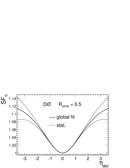
Figure 16: Parameterization for the scale factor $SF_{\eta}^{\textnormal{}}$ resulting from the global fit to the relative MPF response measurements in data for ${\mathcal{R}_{\textnormal{cone}}}=0.5$ jets. The dashed lines illustrate the statistical uncertainty band.

This procedure reduces the total number of free parameters in data from 264 to less than 60, which are determined from the global fit.

Figure 15 shows two examples of the global fit result in data for ${\mathcal{R}_{\textnormal{cone}}}=0.5$ jets. The dashed and continuous lines represent $F_{\eta}^{\textnormal{{${\gamma}+\textnormal{jet}$}}}$ (including background contamination) and $F_{\eta}^{\textnormal{{$\textnormal{dijet}$}}}$, as shown respectively in the upper and lower branch of Eq. 43. As in the case of the absolute response, the relative response is very similar for jets with ${\mathcal{R}_{\textnormal{cone}}}=0.5$ and $0.7$.

9.2 Results

The relative response $F_{\eta}^{\textnormal{{${\gamma}+\textnormal{jet}$}}}$ as derived by the global fit describes the average response of the jets as produced by the ${\gamma}+\textnormal{jet}$ processes. The correction $F_{\eta}^{\textnormal{{$\textnormal{dijet}$}}}$ can be used for samples where the parton final state is closer to that of dijet processes.

Figure 17 presents the final relative MPF response correction in data for ${\mathcal{R}_{\textnormal{cone}}}=0.5$ jets for selected values of $E^{\prime}$. This figure illustrates the non-uniform response of the calorimeter as a function of ${\eta_{\textnormal{det}}^{\textnormal{}}}$, especially in the ICR, with its complex geometry and rapid variation of amount of inactive material in front of the calorimeter (see Sec. 5.1.3). The measured relative MPF response for ${\mathcal{R}_{\textnormal{cone}}}=0.7$ jets is very similar.

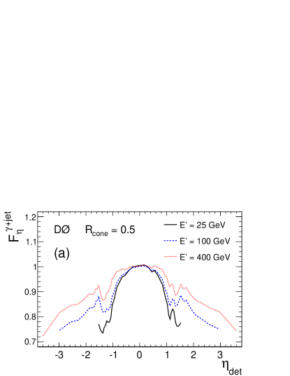
(a)

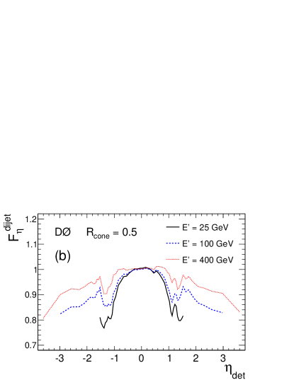
(b)

Figure 17: Relative MPF response correction in data for ${\mathcal{R}_{\textnormal{cone}}}=0.5$ jets as function of $\eta_{\textnormal{det}}^{\textnormal{}}$ and separately for LABEL:sub@feta_esummary_data_jccb_gamjet ${\gamma}+\textnormal{jet}$ ($F_{\eta}^{\textnormal{{${\gamma}+\textnormal{jet}$}}}$) and LABEL:sub@feta_esummary_data_jccb_dijet dijet ($F_{\eta}^{\textnormal{{$\textnormal{dijet}$}}}$) events, as given in Eq. 43. Each line corresponds to a different value of $E^{\prime}$ as indicated.

A self-consistency test is performed to verify the effectiveness of the parametrized $\eta$-dependent jet response in correcting the jet energies. The same samples used in the derivation of $F_{\eta}^{\textnormal{}}$, ${\gamma}+\textnormal{jet}$ and dijet, are split into $\Delta{\eta_{\textnormal{det}}^{\textnormal{}}}=0.4$ subsamples, wider than in the derivation, in order to achieve higher statistical precision. For the test, the ${\not\!\!{E^{\textnormal{}}_{\textnormal{T}}}}$ used for the MPF (Eq. 12) is corrected using $F_{\eta}^{\textnormal{}}$ from the global fit, and then $F_{\eta}^{\textnormal{}}$ is measured again. The result is a residual $F_{\eta}^{\textnormal{}}$ correction that is expected to be consistent with unity. An example of the consistency test with ${\mathcal{R}_{\textnormal{cone}}}=0.5$ jets is displayed in Fig. 18. An additional uncertainty is added to the relative MPF response to cover the presence of the small residual $F_{\eta}^{\textnormal{}}$. This uncertainty is also shown in Fig. 18.

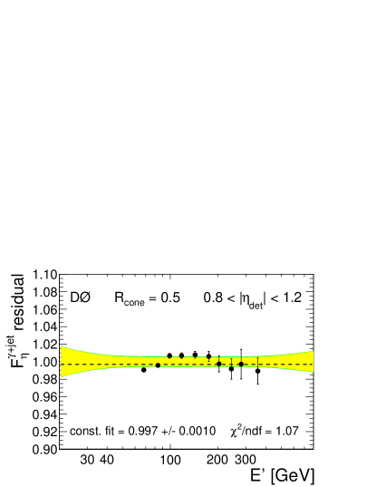
Figure 18: (color online) Residual $F_{\eta}^{\textnormal{}}$ for ${\mathcal{R}_{\textnormal{cone}}}=0.5$ jets in ${\gamma}+\textnormal{jet}$ data as a function of $E^{\prime}$ for $0.8\leq{\left|{{\eta_{\textnormal{det}}^{\textnormal{}}}}\right|}<1.2$. The yellow shaded band represents the statistical uncertainty from the global fit, while the green band shows the additional uncertainty described in Sec. 9.2.

9.3 Uncertainties

The systematic uncertainties on the relative response for the ${\gamma}+\textnormal{jet}$ sample ($F_{\eta}^{\textnormal{{${\gamma}+\textnormal{jet}$}}}$) include the residual $F_{\eta}^{\textnormal{}}$ correction (Sec. 9.2) and the uncertainty on the correction for background contamination (Sec. 8.3.2). The systematic uncertainties on $F_{\eta}^{\textnormal{dijet}}$ also include the residual $F_{\eta}^{\textnormal{}}$ correction, plus uncertainties from resolution bias correction and high energy extrapolation (described in Ref. [4]).

Figure 19 shows as an example the summary of the uncertainties on the response correction for ${\gamma}+\textnormal{jet}$ data, including contributions from the absolute response (Sec. 8.5), the statistical uncertainty on $F_{\eta}^{\textnormal{{${\gamma}+\textnormal{jet}$}}}$ from the global fit, and the combination of the systematic uncertainties on $F_{\eta}^{\textnormal{{${\gamma}+\textnormal{jet}$}}}$. Uncertainty on $F_{\eta}^{\textnormal{dijet}}$ are typically of similar size as for $F_{\eta}^{\textnormal{photonjet}}$, being a little smaller for high $\left|{{\eta_{\textnormal{det}}^{\textnormal{}}}}\right|$ and larger energy, where larger dijet statistics is available.

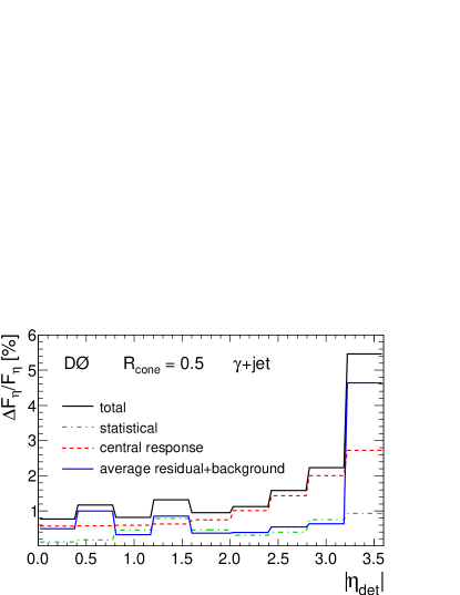
Figure 19: Uncertainties on the relative MPF response correction in ${\gamma}+\textnormal{jet}$ data for ${\mathcal{R}_{\textnormal{cone}}}=0.5$ jets, as a function of ${\left|{{\eta_{\textnormal{det}}^{\textnormal{}}}}\right|}$ for ${p^{\prime}_{\textnormal{T}}}={50\mskip 4.0mu plus 2.0mu minus 2.5mu\textnormal{$\textnormal{GeV}$}}$. The bold solid line shows the total uncertainty, split into individual contributions: statistical, average residual and background correction combined, and central response correction.

10 MPF response bias corrections

The determination of the MPF response suffers from three main biases (see Sec. 5.2) that need to be corrected to recover the true jet response. The first bias affects the response measurement in data only, and is related to the imperfect calibration of the measured photon $p^{\textnormal{}}_{\textnormal{T}}$ as well as the presence of dijet background contamination in the selected ${\gamma}+\textnormal{jet}$ sample. The correction for this bias was discussed in Sec. 8.3.2. This section presents the correction for the other two biases: from zero suppression and from event topology, that affect the determination of response in both data and MC.

10.1 Zero-suppression bias correction

Zero suppression, which introduces the bias on the offset energy estimator described in Sec. 7.4, also biases the estimator of the MPF response. Since the cells in the jet cone are more likely to pass the suppression threshold than those outside the cone, the ${\not\!\!{E^{\textnormal{}}_{\textnormal{T}}}}$ in the direction of the jet is reduced, artificially increasing the estimated MPF response.

In analogy with ${k_{\textnormal{O}}^{\textnormal{ZS}}}$ in Sec. 7.4, a correction factor for the MPF response, ${k_{\textnormal{R}}^{\textnormal{ZS}}}$, is also estimated in MC using ${\gamma}+\textnormal{jet}$ samples where the same generator-level events are processed with and without ZB overlay. The correction factor is defined in Eq. 18.

This factor is measured using the events selected with the same kinematic cuts as for ${k_{\textnormal{O}}^{\textnormal{ZS}}}$ determination with the exception that the events should contain exactly one jet and exactly one photon back-to-back to the jet with $\left|{\Delta{\phi}({\gamma},\textnormal{jet})}\right|>{3.0\mskip 4.0mu plus 2.0mu minus 2.5mu\textnormal{rad}}$, and either one or two reconstructed PVs, following the requirements used in the derivation of the MPF response.

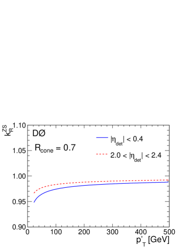
Figure 20: ${k_{\textnormal{R}}^{\textnormal{ZS}}}$ correction factor as a function of $p^{\prime}_{\textnormal{T}}$ for ${\mathcal{R}_{\textnormal{cone}}}=0.7$ jets in two different $\left|{{\eta_{\textnormal{det}}^{\textnormal{}}}}\right|$ regions.

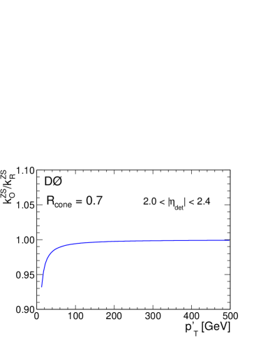
Figure 21: ${{k_{\textnormal{O}}^{\textnormal{ZS}}}}/{{k_{\textnormal{R}}^{\textnormal{ZS}}}}$ correction factor as a function of $p^{\prime}_{\textnormal{T}}$ for ${\mathcal{R}_{\textnormal{cone}}}=0.7$ jets in $2.0<{\left|{{\eta_{\textnormal{det}}^{\textnormal{}}}}\right|}<2.4$.

An example of the response correction factor for ${\mathcal{R}_{\textnormal{cone}}}=0.7$ jets is shown in Fig. 20 for two different $\left|{{\eta_{\textnormal{det}}^{\textnormal{}}}}\right|$ regions. The correction factor for ${\mathcal{R}_{\textnormal{cone}}}=0.5$ jets is almost identical.

The bias arising from the zero-suppression effect on the MPF response is highly correlated with the bias on the offset estimation discussed in Sec. 7.4. Both are smaller than unity and have the same magnitude (e.g., compare Fig. 8 and Fig. 20), and therefore they partially cancel in the overall response correction. It is convenient to parametrize the ${{k_{\textnormal{O}}^{\textnormal{ZS}}}}/{{k_{\textnormal{R}}^{\textnormal{ZS}}}}$ ratio, which enters Eq. 9 directly. As an example, Fig. 21 illustrates the extracted ${{k_{\textnormal{O}}^{\textnormal{ZS}}}}/{{k_{\textnormal{R}}^{\textnormal{ZS}}}}$ factor as a function of $p^{\prime}_{\textnormal{T}}$ for $2.0<{\left|{{\eta_{\textnormal{det}}^{\textnormal{}}}}\right|}<2.4$. The variation of the ${{k_{\textnormal{O}}^{\textnormal{ZS}}}}/{{k_{\textnormal{R}}^{\textnormal{ZS}}}}$ correction is within 1% over the e$\left|{{\eta_{\textnormal{det}}^{\textnormal{}}}}\right|$ range.

10.2 Topology bias correction

After applying the two bias corrections above, the MPF estimate of the response to the hadronic recoil against the particle-level photon may still differ from the true jet response due to a number of physics and instrumental effects. The goal of the topological bias correction is to compensate for the net effect of all the remaining contributions.

An example of physics-related bias is soft radiation below the jet reconstruction threshold of ${p^{\textnormal{}}_{\textnormal{T}}}={6\mskip 4.0mu plus 2.0mu minus 2.5mu\textnormal{GeV}}$, despite the stringent ${\gamma}+\textnormal{jet}$ selection requiring exactly one jet and $\left|{\Delta{\phi}({\gamma},\textnormal{jet})}\right|>{3.0\mskip 4.0mu plus 2.0mu minus 2.5mu\textnormal{rad}}$. This can spoil the $p^{\textnormal{}}_{\textnormal{T}}$ balance between the jet and the photon. Depending on whether such radiation populates the photon or jet hemispheres, the estimated MPF response can be higher or lower than the true jet response. Another example is the fact that, owing to the shrinkage of the rapidity space shrinking in angle of constant intervals of rapidity (especially for forward jets), the hadronic recoil can cover significantly larger physical space than the reconstructed jet. Since the particles outside the jet cone are of lower energy than in the core, the estimated MPF response is a priori lower than the actual response to the jet. This difference can also be increased by the larger effect of zero suppression on low energy calorimeter deposits. Finally, the MPF method inherently relies on $p^{\textnormal{}}_{\textnormal{T}}$ balance and therefore is in principle more suitable for jet $p^{\textnormal{}}_{\textnormal{T}}$, rather than energy, calibration. The difference between jet $p^{\textnormal{}}_{\textnormal{T}}$ and energy calibration is the largest for low energy jets, where jets are wider and mass effects can be sizable. The MPF method can absorb instrumental effects unrelated to energy calibration, such as the rapidity bias in the ICD region (see Sec. 16.3).

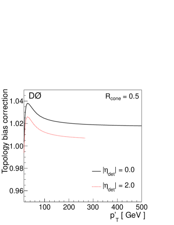
Figure 22: Example of the topology bias correction $k_{\textnormal{R}}^{\textnormal{topo}}$ for ${\mathcal{R}_{\textnormal{cone}}}=0.5$ jets at ${\left|{{\eta_{\textnormal{det}}^{\textnormal{}}}}\right|}=0$ and $2$. The lines represent the result of a smooth parameterization of the correction.

The net bias correction factor, denoted by $k_{\textnormal{R}}^{\textnormal{topo}}$, is estimated from ${\gamma}+\textnormal{jet}$ MC samples without ZB overlay, selected using the same criteria as for the absolute response measurement (Sec. 8.1). As indicated in Eq. 19, it is defined as the ratio of the true jet response (Eq. 6) and the MPF response with respect to the particle-level photon (Eq. 29). The true jet response is estimated as the ratio of the average visible energy in the calorimeter from particles belonging to the particle jet to the average particle jet energy (the particle jet is required to match the direction of the reconstructed jet within ${\Delta\mathcal{R}}<{\mathcal{R}_{\textnormal{cone}}}/2$). Figure 22 shows an example of the topology bias corrections for ${\mathcal{R}_{\textnormal{cone}}}=0.5$ jets at ${\left|{{\eta_{\textnormal{det}}^{\textnormal{}}}}\right|}=0$ and $2$. The corrections for ${\mathcal{R}_{\textnormal{cone}}}=0.7$ are closer to unity. These corrections are also derived from a MC simulation using a tuned single particle response (see Sec. 14), to be applied to jets in data. We assign a systematic uncertainty that covers the difference between the topology bias correction for the standard MC and the MC with the tuned single particle response. This difference is smaller than $0.5\%$ for central jets and up to $\approx 1\%$ for forward jets. The list of uncertainties also includes the statistical uncertainty ($\lesssim 0.5\%$) and systematic uncertainty from varying the matching criterion between the reconstructed and particle jets ($0.2\%-0.5\%$), varying the hadron response, and considering alternative physics models, as described below.

The particle-level $p^{\textnormal{}}_{\textnormal{T}}$ balance in ${\gamma}+\textnormal{jet}$ events can be modified by initial and final state radiation or by additional soft radiation caused by spectator parton interactions (“soft underlying event”). To estimate model dependence, the $k_{\textnormal{R}}^{\textnormal{topo}}$ correction is obtained using three sets of pythia parameters, called Tune A, Tune B and Tune DWT. Tune A and B are tuned to the CDF Run I data [36]. Tune A allows for more initial state radiation than Tune B. Consequently, the contribution of the soft underlying event is smaller in Tune A than in Tune B. D0 Run II data on dijet azimuthal decorrelations [40] show a lack of sufficient initial state radiation in Tune B while there is too much radiation in Tune A. Tune DWT [42] has been developed to provide an improved description of this observable. The systematic uncertainty due to physics modeling has been estimated as the maximum observed difference with respect to pythia Tune A. It is smaller than $0.4\%$ for central jets, increasing up to $2\%-3$% for forward jets.

11 Showering correction

After implementing the offset and full set of response corrections discussed in Secs. 7, 8, 9 and 10, the corrected jet energy does not yet correspond to the particle-jet energy. Indeed, after offset subtraction, not all the energy contained inside the jet cone originates from particles belonging to the particle jet, so the response correction can not recover the original particle jet energy. Particles not belonging to the particle jet (e.g., from the underlying event) may contribute to the energy inside the jet cone, due to effects such as the shower development from interactions with the detector material, the granularity and pseudo-projective arrangement of the calorimeter towers, as well as the bending of low momentum charged particles in the magnetic field. The same instrumental effects also cause some of the energy from particles belonging to the particle jet to leak outside the jet cone. Therefore, a “showering correction” is required to compensate for the net energy flow through the jet cone boundary. Such a correction must be defined in a way consistent with the rest of corrections to ensure that the particle jet energy is recovered. The definition of this showering correction is given as $S$ in Eq. 7.

11.1 Method

The showering correction is determined both in data and MC using ${\gamma}+\textnormal{jet}$ events selected using the same criteria as for the absolute response measurement (see Sec. 8.1), with the exception that the probe jet is not restricted to be in the central calorimeter. The procedures to estimate the showering correction in data and MC are different. In the case of MC, it is possible to directly obtain an unbiased estimator of the true showering correction. In the case of data, an observable sensitive to the jet showering must be defined, resulting in a potentially biased estimator of the showering correction. The estimator must be calibrated to remove the bias. The following sections present an overview of both procedures.

11.1.1 Monte Carlo method

In the case of MC, the showering correction is estimated in simulated ${\gamma}+\textnormal{jet}$ events without ZB overlay (i.e., with no offset energy). Since detailed information is available in the simulation regarding the amount of energy deposited in each calorimeter cell by each particle, it is possible to directly estimate $S$ according to Eq. 7. In the absence of offset effects, the numerator of the showering correction represents the uncorrected jet energy as determined by the jet algorithm. The denominator is estimated by adding the visible energy in all the calorimeter cells from the particles originating from the particle jet. Therefore, the measurement of $S$ in MC requires a spatial matching between the calorimeter probe jet and the particle jet that is required to be within ${\Delta\mathcal{R}}<{\mathcal{R}_{\textnormal{cone}}}/2$.

11.1.2 Template-based method

The measurement of the showering correction in data is based on examining the energy distributions in the calorimeter in annuli of increasing radius ${\Delta\mathcal{R}}$ with respect to the jet axis. We refer to such distributions as the “jet energy profile”. These are obtained by combining cells into towers following exactly the same procedure as the jet algorithm (see Par. 3.2.2), and then adding the energy from all towers within a particular ${\Delta\mathcal{R}}$ annulus.

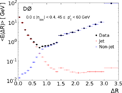
Figure 23: Jet energy profiles as a function of distance from the jet axis ${\Delta\mathcal{R}}$ for MC and data. The jets in data are corrected for offset energy from noise and additional $p\bar{p}$ collisions and are compared to MC jets without offset (called “jet” on the plot) and contributions from the underlying event (“non-jet”). The MC templates are weighted with their fractions obtained from the fit to data.

Figure 23 shows an example of the jet energy profile for central jets in ${\gamma}+\textnormal{jet}$ data and MC without ZB overlay. Exploiting the available MC information, it is possible to compute the energy profiles corresponding to the particles belonging to the particle jet matching the reconstructed jet (“particle-jet profile”) and the rest of the particles (“non-particle-jet profile”). The latter receives contributions from the underlying event as well as particles resulting from large-angle gluon radiation during the parton shower evolution. This figure helps to visualize the need for the showering correction. The integral of the total reconstructed jet profile up to ${\Delta\mathcal{R}}={\mathcal{R}_{\textnormal{cone}}}$, $E^{\textnormal{meas}}_{\textnormal{}}$, represents the uncorrected jet energy as reconstructed by the jet algorithm, which receives contributions from both particle-jet and non-particle-jet profiles:

$${E^{\textnormal{meas}}_{\textnormal{}}}\!=\!{E^{\textnormal{meas}}_{\textnormal{ptclj}}}({\Delta\mathcal{R}}\!\!=\!\!{\mathcal{R}_{\textnormal{cone}}})+{E^{\textnormal{meas}}_{\textnormal{non-ptclj}}}({\Delta\mathcal{R}}\!\!=\!\!{\mathcal{R}_{\textnormal{cone}}}).$$ (45)

On the other hand, the integral of the particle-jet profile, ${E^{\textnormal{meas}}_{\textnormal{ptclj}}}(\text{all}\,{\Delta\mathcal{R}})$, represents the total visible energy from the particle jet, a small fraction of which is deposited beyond the jet cone boundary. The ratio of the two integrals represents an estimator of the true showering correction:

$$\hat{S}=\frac{{E^{\textnormal{meas}}_{\textnormal{}}}}{{E^{\textnormal{meas}}_{\textnormal{ptclj}}}(\text{all}\,{\Delta\mathcal{R}})},$$ (46)

where ${E^{\textnormal{meas}}_{\textnormal{}}}$ is defined in Eq. 45. The distinct spatial distribution of energy around the jet centroid for each of these two contributions, as shown in Fig. 23, suggests that the showering correction can be estimated from a fit to the total jet profile, using the particle-jet and non-particle-jet profiles extracted from MC as templates. This requires a good description of the jet profile in the MC, including proper modeling of both the physics and instrumental effects. The ${\gamma}+\textnormal{jet}$ MC samples used are generated using pythia Tune A [36], which has been verified to successfully describe the jet shapes in inclusive jet production [37]. The level of agreement observed in this measurement confirms this is also the case in ${\gamma}+\textnormal{jet}$ events.

It is also necessary to include a template describing the offset energy profile. Such an offset template is estimated in ${\gamma}+\textnormal{jet}$ MC by subtracting from each template in the sample including unsuppressed ZB overlay the corresponding template in the sample without ZB overlay. This takes into account distortions to the template shape related to the interplay between zero-suppression and the presence of offset energy. Since the overlay in MC is based on ZB data events, the estimated offset profile is expected to closely match the one in data. The three profiles obtained using the particle-jet, non-particle-jet and offset templates are fitted to data to determine the contributions of $E_{\textnormal{ptclj}}^{\textnormal{meas}}({\Delta\mathcal{R}}={\mathcal{R}_{\textnormal{cone}}})$ and $E_{\textnormal{non-ptclj}}^{\textnormal{meas}}({\Delta\mathcal{R}}={\mathcal{R}_{\textnormal{cone}}})$. Figure 23 compares the spatial energy profiles in data with subtracted offset contribution and the MC templates. The MC templates are weighted with their fractions obtained from the maximum likelihood fit to data. We see that MC describes the data well when both the energies inside and outside the jet are considered.

The procedure has been validated in full MC, where the estimated showering correction is found to closely match the true showering correction estimated following the procedure described in Sec. 11.1.1. To take into account any potential bias in the method, the final value of the showering correction in data is computed as

$$S_{\textnormal{data}}=\hat{S}_{\textnormal{data}}\cdot\frac{S_{\textnormal{MC}}^{\textnormal{true}}}{\hat{S}_{\textnormal{MC}}},$$ (47)

where the true showering correction $S_{\textnormal{MC}}^{\textnormal{true}}$ is directly available in MC and estimated following the procedure described in Sec. 11.1.1, and $\hat{S}_{\textnormal{MC}}$ and $\hat{S}_{\textnormal{data}}$ are the template-based showering corrections in MC and data, respectively. The resulting bias is small (typically less than $0.5\%$), and a correction is made to ensure a properly calibrated estimator in data.

11.2 Results

Figure 24 presents the estimated showering corrections for ${\mathcal{R}_{\textnormal{cone}}}=0.5$ jets in data, as a function of $p^{\prime}_{\textnormal{T}}$ and for different $\eta_{\textnormal{det}}^{\textnormal{}}$ bins. The showering corrections in data are in good agreement with MC. This motivates parameterizing the correction in data using the same energy dependence as observed in MC.

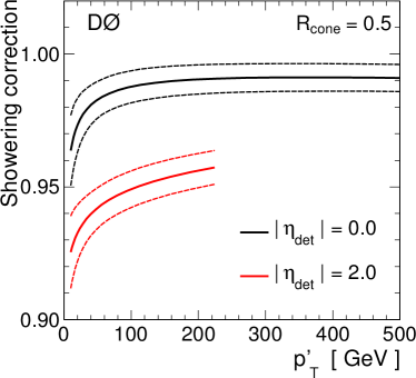
Figure 24: Showering correction for ${\mathcal{R}_{\textnormal{cone}}}=0.5$ jets in data, as a function of $p^{\prime}_{\textnormal{T}}$ and for two $\eta_{\textnormal{det}}^{\textnormal{}}$ values, ${\left|{{\eta_{\textnormal{det}}^{\textnormal{}}}}\right|}=0$ and ${\left|{{\eta_{\textnormal{det}}^{\textnormal{}}}}\right|}=2$. The lines represent the results of a smooth parameterization of the correction.

The uncertainties on the showering correction are typically less than $1.5\%$ (slightly larger for smaller $p^{\textnormal{}}_{\textnormal{T}}$) of the overall correction factor. The main sources of uncertainty come from the difference between data and MC in the single particle response at low $p^{\textnormal{}}_{\textnormal{T}}$, the quality of the fits of MC templates to data, and the description of the underlying event determined by using alternative pythia tunes.

12 Summary of corrections and uncertainties

12.1 Mapping of measured energy to $E^{\prime}$

The individual corrections discussed in previous sections have all been parametrized and evaluated as a function of $E^{\prime}$ or $p^{\prime}_{\textnormal{T}}$ (see Eq. 15). Using the uncorrected jet energy ($E^{\textnormal{meas}}_{\textnormal{}}$), the mapping to ${E^{\prime}}$ is found by solving the following equation (cf. Eq. 9) for $E^{\prime}$:

$$\begin{aligned} {E^{\textnormal{corr}}_{\textnormal{}}}&=\frac{{E^{\textnormal{meas}}_{\textnormal{}}}-\hat{E}_{\textnormal{O}}}{{R_{\textnormal{MPF}}^{\textnormal{{${\gamma}+\textnormal{jet}$}}}}\left({E^{\prime}}\right){k_{\textnormal{R}}^{\textnormal{topo}}}\left({E^{\prime}}\right)S\left({E^{\prime}}\right)}\frac{{{k_{\textnormal{O}}^{\textnormal{ZS}}}}\left({E^{\prime}}\right)}{{{k_{\textnormal{R}}^{\textnormal{ZS}}}}\left({E^{\prime}}\right)}\\ &={E^{\prime}}\,{C}\left({E^{\prime}}\right),\end{aligned}$$ (48)

implying the dependence on $\eta$. After $E^{\prime}$ is iteratively extracted from the last two members of the equation, the corrected jet energy $E^{\textnormal{corr}}_{\textnormal{}}$, that represents the particle jet energy $E^{\textnormal{ptcl}}_{\textnormal{}}$, can be computed directly. The quantity ${C}={E^{\textnormal{ptcl}}_{\textnormal{}}}/{E^{\prime}}$ is estimated in ${\gamma}+\textnormal{jet}$ MC as a function of $E^{\prime}$ and $\eta_{\textnormal{det}}^{\textnormal{}}$, separately for ${\mathcal{R}_{\textnormal{cone}}}=0.7$ and $0.5$ jets. This factor is interpreted as the fraction of energy lost from out-of-cone radiation (physics showering), since it compares the particle-jet energy, confined by the geometry of the jet, to $E^{\prime}$, the estimated energy of the parton recoiling against the photon in an ideal $2\to 2$ process. As expected, ${C}<1$, especially for ${\mathcal{R}_{\textnormal{cone}}}=0.5$ and/or forward jets, where values as low as $0.85-0.9$ are reached. Since the different correction components depend logarithmically on the energy, a precision of $5\%$ or better is sufficient in this mapping from $E^{\textnormal{meas}}_{\textnormal{}}$ to $E^{\prime}$.

To verify the precision of the mapping, $E^{\prime}$, as estimated via Eq. 48, is compared to the true $E^{\prime}$ in ${\gamma}+\textnormal{jet}$ MC. The mapping is found to be precise to better than $3\%$ over the full $\eta_{\textnormal{det}}^{\textnormal{}}$ range.

12.2 Results: corrections and uncertainties

This section presents a few representative examples of the total correction factors obtained with the methods described in Secs. 7, 8, 9, 10 and 11 for D0 data and MC simulation.

Separate corrections and uncertainties are extracted for data and simulation, for each of the jet cone sizes ${\mathcal{R}_{\textnormal{cone}}}=0.5$ and $0.7$, and for the five different run periods (see Sec. 6.1). Figure 25 shows the typical JES correction factor ${E^{\textnormal{ptcl}}_{\textnormal{}}}/{E^{\textnormal{meas}}_{\textnormal{}}}$ for jets with ${\mathcal{R}_{\textnormal{cone}}}=0.5$ in two run periods, Run IIa ($1.1\mskip 4.0mu plus 2.0mu minus 2.5mu\textnormal{$\textnormal{fb}^{-1}$}$) and Run IIb2 ($3.0\mskip 4.0mu plus 2.0mu minus 2.5mu\textnormal{$\textnormal{fb}^{-1}$}$), taken as examples throughout this section. The value of the correction spans a range of less than 10% in most of the detector. The structures in the ICD region of the calorimeter ($1.0<{\left|{{\eta_{\textnormal{det}}^{\textnormal{}}}}\right|}<1.6$) reflect the reduced coverage and additional passive material, and the different response in the forward region of the calorimeter (${\left|{{\eta_{\textnormal{det}}^{\textnormal{}}}}\right|}>3$) is evident. The overall difference between the two periods is a consequence of the modified jet-finding algorithm (see Sec. 3.2.2) and calorimeter calibration.

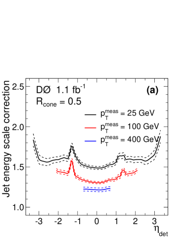
(a)

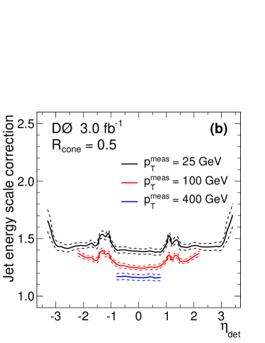
(b)

Figure 25: Jet energy scale corrections, ${E^{\textnormal{ptcl}}_{\textnormal{}}}/{E^{\textnormal{meas}}_{\textnormal{}}}$, for data jets with ${\mathcal{R}_{\textnormal{cone}}}=0.5$ in LABEL:sub@fig:Summary_CorrVsEta_JCCB_DATA_IIA Run IIa and LABEL:sub@fig:Summary_CorrVsEta_JCCB_DATA_IIB2 Run IIb2 as a function of $\eta_{\textnormal{det}}^{\textnormal{}}$ for different uncorrected jet $p^{\textnormal{}}_{\textnormal{T}}$ values ($p^{\textnormal{meas}}_{\textnormal{T}}$). Dashed lines show the total systematic uncertainty on the corrections.

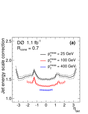
(a)

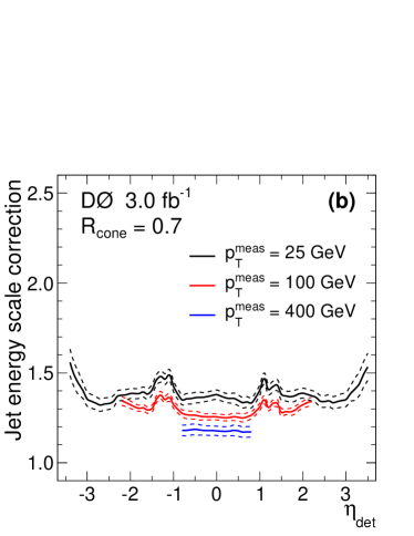
(b)

Figure 26: Same as in Fig. 25, but for ${\mathcal{R}_{\textnormal{cone}}}=0.7$.

The correction factor for ${\mathcal{R}_{\textnormal{cone}}}=0.7$ jets (Fig. 26) exhibits the same features as for ${\mathcal{R}_{\textnormal{cone}}}=0.5$. The absolute value of the correction is slightly smaller for ${\mathcal{R}_{\textnormal{cone}}}=0.7$ jets, reflecting the better geometric coverage provided by the larger cone radius. This is more evident for low energy jets, whose particle showers are less boosted and correspondingly less well collimated. Figure 27 shows the uncertainty on the correction for ${\mathcal{R}_{\textnormal{cone}}}=0.5$ jets in the same two run periods, split into their independent contributions. The uncertainties for ${\mathcal{R}_{\textnormal{cone}}}=0.7$ are similar.

The leading contribution to the uncertainty comes from the correction on the jet response. At low energy, the offset energy subtraction and the out-of-cone correction contribute significantly. As the energy of the jet increases, the offset energy becomes a smaller fraction of the measured energy and the corresponding uncertainty less relevant. The largest contribution to the uncertainty on the response comes from the absolute response, which suffers from large statistical uncertainties from extrapolation into regions not covered by ${\gamma}+\textnormal{jet}$ data (very low and high energies).

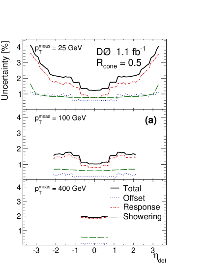
(a)

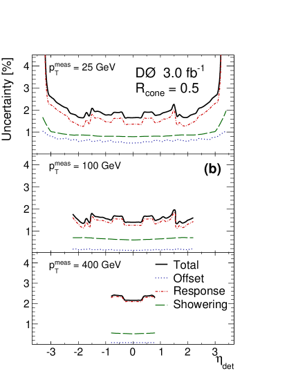
(b)

Figure 27: Jet energy scale uncertainty for data jets with ${\mathcal{R}_{\textnormal{cone}}}=0.5$, in LABEL:sub@fig:Summary_ErrVsEta_JCCB_DATA_IIA Run IIa and LABEL:sub@fig:Summary_ErrVsEta_JCCB_DATA_IIB2 Run IIb2 as a function of $\eta_{\textnormal{det}}^{\textnormal{}}$ for different uncorrected jet $p^{\textnormal{}}_{\textnormal{T}}$ ($p^{\textnormal{meas}}_{\textnormal{T}}$).

Figure 28 shows an example of jet energy scale correction and uncertainty for MC events. The simplified model in the MC simulation yields a more uniform correction versus $\eta_{\textnormal{det}}^{\textnormal{}}$ as compared with data. The overall uncertainty for simulation is smaller than for data, while the uncertainty for the offset energy correction, being completely data-driven, is very similar.

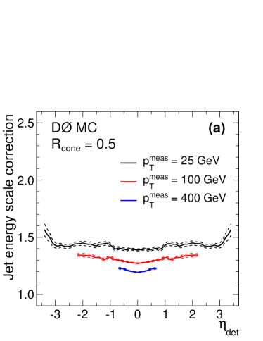
(a)

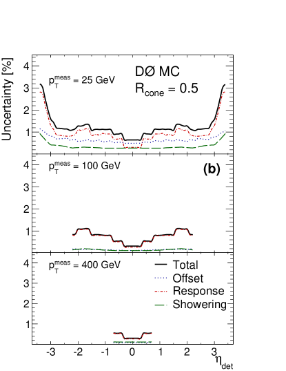
(b)

Figure 28: Jet energy scale LABEL:sub@fig:Summary_CorrVsEta_JCCB_MC_IIB2 correction, ${E^{\textnormal{ptcl}}_{\textnormal{}}}/{E^{\textnormal{meas}}_{\textnormal{}}}$, and LABEL:sub@fig:Summary_ErrVsEta_JCCB_MC_IIB2 uncertainty for jets in MC simulation with ${\mathcal{R}_{\textnormal{cone}}}=0.5$, in Run IIb2 as a function of $\eta_{\textnormal{det}}^{\textnormal{}}$ for different uncorrected jet $p^{\textnormal{}}_{\textnormal{T}}$ ($p^{\textnormal{meas}}_{\textnormal{T}}$).

13 Closure tests

This section presents results on the validation of the jet energy scale corrections and thei uncertainties. These validation tests are referred to as “closure tests,” and their goal is to assess whether the corrections calibrating jet energy back to the particle level are within the quoted uncertainties.

To assess whether closure of the corrections is achieved, observables able to probe the relationship between the particle and (calibrated) calorimeter jet energies must be defined. In the case of MC this can be straightforward. In the case of data, the connection is not direct and effects not related to jet energy calibration (e.g., background contamination, photon energy scale) must be taken into account.

13.1 Sample selection

Since closure tests are mainly designed to probe the absolute energy scale calibration, a natural sample to use is ${\gamma}+\textnormal{jet}$ events. The event selections used for the closure tests closely follow those used for the absolute response measurement (Sec. 8.1), except that no limit is imposed on the number of vertices or jet multiplicity. Considering events with ${n_{\textnormal{PV}}}\geq 1$ enforces consistency with the determination of the offset bias correction ${k_{\textnormal{O}}^{\textnormal{ZS}}}$, which is estimated for the inclusive (${n_{\textnormal{PV}}}\geq 1$) sample. There are two reasons for allowing events with more than one jet. First, typical event selections in physics analyses consider final states inclusive in the number of jets. Second, keeping events with extra jets minimizes biases in the average offset, since some of those jets will likely arise from additional parton interactions [43].

Closure tests are performed separately for ${\mathcal{R}_{\textnormal{cone}}}=0.7$ and $0.5$ jets, in different $0.4$-wide bins of ${\left|{{\eta_{\textnormal{det}}^{\textnormal{}}}}\right|}$ (up to ${\left|{{\eta_{\textnormal{det}}^{\textnormal{}}}}\right|}<3.6$) and as a function of $p^{\prime}_{\textnormal{T}}$ (defined in Sec. 7.4).

Due to a finite jet energy resolution around the uncorrected $p^{\textnormal{}}_{\textnormal{T}}$ reconstruction threshold of $6\mskip 4.0mu plus 2.0mu minus 2.5mu\textnormal{$\textnormal{GeV}$}$, the $E/{p^{\textnormal{}}_{\textnormal{T}}}$ of the jet increases as compared with the particle level jet. This effect is especially large for lower jet $p^{\textnormal{}}_{\textnormal{T}}$ (the “low-$p^{\textnormal{}}_{\textnormal{T}}$ bias”), and can be reduced by the additional requirement of ${p^{\textnormal{}}_{\textnormal{T{$\gamma$}}}}\geq{30\mskip 4.0mu plus 2.0mu minus 2.5mu\textnormal{GeV}}$, applied in the closure test. However, even for events with exactly one jet, the low-$p^{\textnormal{}}_{\textnormal{T}}$ bias with a jet located in or around the ICD region is still present above $30\mskip 4.0mu plus 2.0mu minus 2.5mu\textnormal{$\textnormal{GeV}$}$, mainly due to poorer jet energy resolution as compared with other rapidity regions.

13.2 Direct closure tests in MC

In the case of MC, the availability of the particle jet information allows the definition of a “direct” closure variable $\left<{{E^{\textnormal{corr}}_{\textnormal{}}}}\right>/\left<{{E^{\textnormal{ptcl}}_{\textnormal{}}}}\right>$ where $E^{\textnormal{corr}}_{\textnormal{}}$ is the corrected jet energy (Eq. 9) and $E^{\textnormal{ptcl}}_{\textnormal{}}$ is the energy of the closest particle jet matching the reconstructed jet within ${\Delta\mathcal{R}}<{\mathcal{R}_{\textnormal{cone}}}/2$. The averages in the ratio $\left<{{E^{\textnormal{corr}}_{\textnormal{}}}}\right>/\left<{{E^{\textnormal{ptcl}}_{\textnormal{}}}}\right>$ are taken for the set of events within the particular $\left({{p^{\prime}_{\textnormal{T}}},{\left|{{\eta_{\textnormal{det}}^{\textnormal{}}}}\right|}}\right)$ bin under consideration.

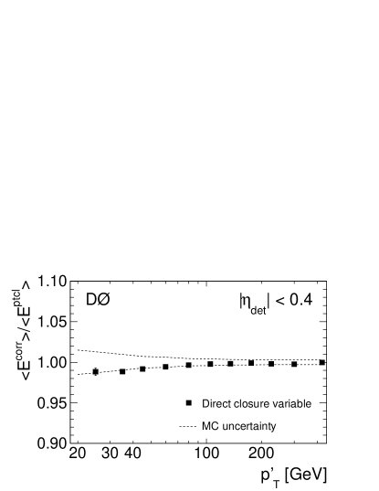
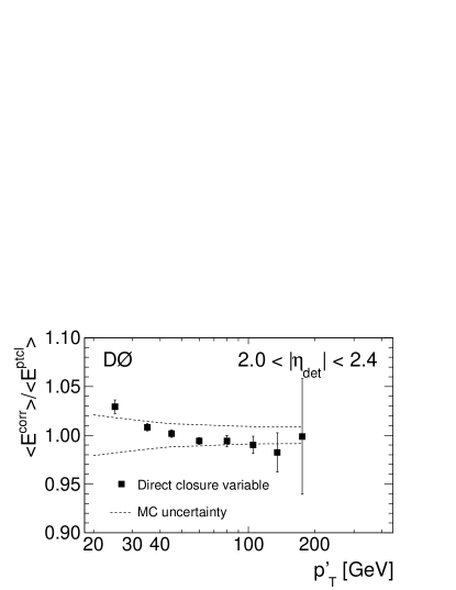
Figure 29: Direct closure variable for ${\mathcal{R}_{\textnormal{cone}}}=0.7$ jets as a function of $p^{\prime}_{\textnormal{T}}$ and in two $\left|{{\eta_{\textnormal{det}}^{\textnormal{}}}}\right|$ regions. The band represents the total uncertainty on the energy scale from the corrections in data and MC added in quadrature.

Figure 29 shows results of direct closure tests for ${\mathcal{R}_{\textnormal{cone}}}=0.7$ in two $\left|{{\eta_{\textnormal{det}}^{\textnormal{}}}}\right|$ bins, taken as an example. The jet energy scale corrections have been evaluated using the internally remapped $E^{\prime}$ (see Eq. 48). The small rise observed at low $p^{\prime}_{\textnormal{T}}$ (mostly at high $|\eta|$) is caused by the low-$p^{\textnormal{}}_{\textnormal{T}}$ bias, as discussed in Sec. 13.1. Taking this into consideration, closure is in general achieved within the quoted $1\%-2\%$ uncertainties.

13.3 Closure tests in data

In contrast with MC, for data there is no possibility to directly check the absolute energy calibration, as no information regarding particle jets is available. Therefore, closure tests are based on the comparison of the corrected jet energies between data and MC. Provided that the jet energy calibration works properly in MC (see Sec. 13.2), it is then possible to relate the data-to-MC intercalibration to the absolute energy calibration in data by reconstructing the particle jet energy, $E^{\textnormal{ptcl}}_{\textnormal{}}$.

As for direct closure in MC, we use ${\gamma}+\textnormal{jet}$ events (Sec. 13.1). The closure observable is defined as the ratio of the average corrected jet energies between data and MC, ${\left.\left<{{E^{\textnormal{corr}}_{\textnormal{data}}}}\right>\middle/\left<{{E^{\textnormal{corr}}_{\textnormal{MC}}}}\right>\right.}$, computed as a function of $p^{\prime}_{\textnormal{T}}$ in different $\left|{{\eta_{\textnormal{det}}^{\textnormal{}}}}\right|$ regions.

Since the goal of the closure tests is to validate the jet energy calibration in pure ${\gamma}+\textnormal{jet}$ events, it is important to properly account for any differences between data and MC which could result in biases in the closure observable. The most relevant effect is related to the presence of dijet background in data. Since the closure observable does not directly involve the reconstructed photon $p^{\textnormal{}}_{\textnormal{T}}$, the main difference results from the flavor composition of the jet. For example, as will be discussed in Sec. 16, low $p^{\textnormal{}}_{\textnormal{T}}$ jets from dijet background are dominated by jets from gluons, whereas jets from ${\gamma}+\textnormal{jet}$ signal are dominated by jets from quarks, and there is up to $8\%$ difference in response for low $p^{\textnormal{}}_{\textnormal{T}}$ jets. In order to account for this bias, data are not compared to pure ${\gamma}+\textnormal{jet}$ MC, but rather to a mixture of ${\gamma}+\textnormal{jet}$ and dijet ($\gamma$-like) MC, combined using the estimated sample purity. This allows a correction for the leading difference between data and MC. Also, the measured photon energy in MC is corrected to ensure its energy scale is consistent with data.

As already indicated, this correction enters the closure test indirectly, via the binning of the closure variable in terms of $p^{\prime}_{\textnormal{T}}$. Figure 30 presents the results of relative data-to-MC closure for ${\mathcal{R}_{\textnormal{cone}}}=0.7$ jets as a function of $p^{\prime}_{\textnormal{T}}$ in two $\left|{{\eta_{\textnormal{det}}^{\textnormal{}}}}\right|$ bins. The corresponding plots for ${\mathcal{R}_{\textnormal{cone}}}=0.5$ jets are shown in Fig. 31. Since a priori jet energy calibration uncertainties for data and MC are largely uncorrelated, the uncertainty on the closure observable is defined as the sum in quadrature of data and MC uncertainties. Data and MC appear intercalibrated, i.e., reproduce $E^{\textnormal{ptcl}}_{\textnormal{}}$ within the estimated uncertainties.

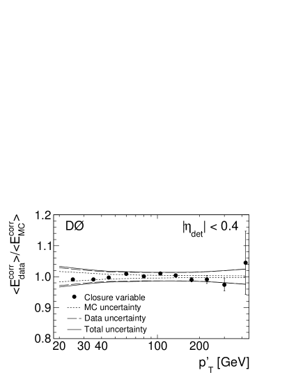
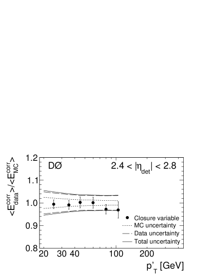
Figure 30: Relative data-to-MC closure variable for ${\mathcal{R}_{\textnormal{cone}}}=0.7$ jets as a function of $p^{\prime}_{\textnormal{T}}$ and in two $\left|{{\eta_{\textnormal{det}}^{\textnormal{}}}}\right|$ bins. The inner and intermediate bands represent the energy scale uncertainty for MC and data, respectively, while the outer band represents the total uncertainty.

Figure 31: Same as on Fig. 30 for jets with ${\mathcal{R}_{\textnormal{cone}}}=0.5$.

14 Flavor-dependent corrections in Monte Carlo

The default jet energy calibration, which is separately derived for data and MC simulations as described in previous sections, corrects the detected jet energies to the particle level, ignoring differences due to the specific flavor of the parton that initiated the jet (known as “jet parton flavor”). As described in Sec. 4.3, samples with different composition than ${\gamma}+\textnormal{jet}$ may require additional corrections to the jet energy scale. An estimation of single-particle responses should reduce the bias in jet energy that arises due to dependence on the jet parton flavor.

The MC simulation evaluates the energy deposited by a jet in the calorimeter summing over the estimated response from all of the particles in the jet. Estimation of single-particle responses should reduce the bias in jet energy that arises due to dependence on the physics process and (more generally) on the jet parton flavor. It would allow measurements to rely on MC simulations to correct for this bias (see e.g., [6]).

This section describes a procedure to tune the MC simulated single-particle response and presents the additional energy correction required for various jet flavors.

14.1 Method

The procedure described below uses single-particle MC samples (see Sec. 14.1.1) and the ${\gamma}+\textnormal{jet}$ and dijet MC and data samples described in Sec. 6. We define a correction factor $F$ for each reconstructed calorimeter jet in the simulation:

$$F=\frac{\sum_{i}E_{i}\cdot R_{i}^{\textnormal{data}}}{\sum_{i}E_{i}\cdot R_{i}^{\textnormal{MC}}},$$ (49)

where the subscript $i$ runs over the particles in the particle jet, $E_{i}$ is the particle energy, and $R_{i}^{\textnormal{data}}$ and $R_{i}^{\textnormal{MC}}$ represent the response to the particle in the calorimeter for data and MC simulation, respectively. To calculate $F$, the particle and calorimeter jets are spatially matched using ${\Delta\mathcal{R}}<{\mathcal{R}_{\textnormal{cone}}}/2$.

To preserve the jet energy scale obtained with ${\gamma}+\textnormal{jet}$ events, we introduce the relative correction factor $F_{\textnormal{corr}}$:

$$F_{\textnormal{corr}}=\frac{1}{\left<{F}\right>_{{{\gamma}+\textnormal{jet}}}}\cdot\frac{\sum_{i}E_{i}\cdot R_{i}^{\textnormal{data}}}{\sum_{i}E_{i}\cdot R_{i}^{\textnormal{MC}}},$$ (50)

where $\left<{F}\right>_{{{\gamma}+\textnormal{jet}}}$ is the average of $F$ in the ${\gamma}+\textnormal{jet}$ sample, parameterized as a function of jet $p^{\textnormal{}}_{\textnormal{T}}$ and $\eta_{\textnormal{det}}^{\textnormal{}}$. The correction factor $F_{\textnormal{corr}}$ is independent of corrections described in the previous sections and can be applied on the jet energy scale corrected jets.

14.1.1 Single-particle response in MC

Single-particle responses in MC are measured from MC samples of single $\gamma$, $e^{\pm}$, $\mu^{\pm}$, $\pi^{\pm}$, $K^{\pm}$, $K^{0}_{\textnormal{S}}$, $K^{0}_{\textnormal{L}}$, $p^{\pm}$, $n$, $\Lambda$, $\Sigma$, and $\Xi$ production simulated with no zero suppression, calorimeter noise, and no ZB overlay. For each particle, the energy of the calorimeter cells contained in the cone with radius ${\mathcal{R}_{\textnormal{cone}}}$ around the particle is summed to obtain the reconstructed energy. The MC single-particle response $R_{i}^{\textnormal{MC}}$ is the ratio between the reconstructed energy and the particle energy. The responses are parameterized versus particle energy and extracted independently for different pseudorapidities. For example, the response to a given hadron $h$ (e.g., $\pi^{+}$) with energy $E$ is parametrized as:

$$R_{\textnormal{h}}^{\textnormal{MC}}=p_{\textnormal{h}}^{(0)}\cdot\left[{1-p_{\textnormal{h}}^{(1)}\cdot(E/0.75)^{p_{\textnormal{h}}^{(2)}-1}}\right],$$ (51)

where $p_{\textnormal{h}}^{(k)}$ are three free parameters for each hadron $h$ that have to be determined. The functional form in Eq. 51 has been varified using MC simulation.

Using MC simulation, we compare the sum of the single particle responses $\sum_{i}E_{i}\cdot R_{i}^{\textnormal{MC}}$ in Eq. 50 with the reconstructed calorimeter jet energy corrected for offset contribution and the offset bias: $({E^{\textnormal{meas}}_{\textnormal{}}}-\hat{E}_{\textnormal{O}})\cdot{k_{\textnormal{O}}^{\textnormal{}}}$. Figure 32 shows that their ratio

$$\frac{{k_{\textnormal{O}}^{\textnormal{}}}({E^{\textnormal{meas}}_{\textnormal{}}}-\hat{E}_{\textnormal{O}})}{\sum_{i}E_{i}\cdot R_{i}^{\textnormal{MC}}}$$ (52)

agrees with unity within 2% for most of the jet energies and pseudorapidities. The residual disagreement is assigned as systematic uncertainty.

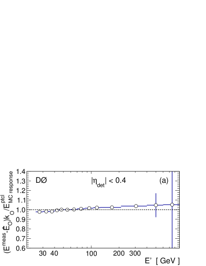
(a)

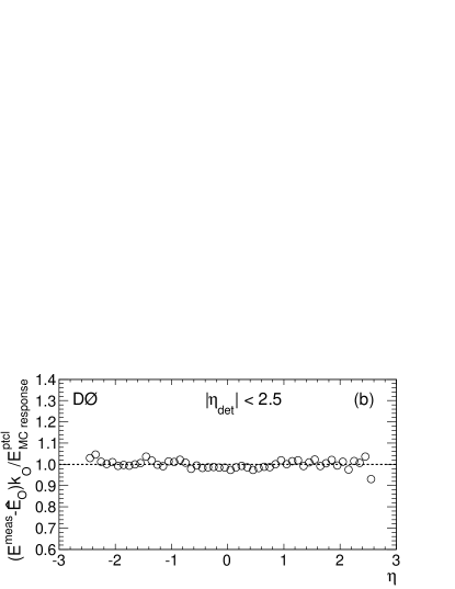
(b)

Figure 32: Ratio between the jet energy as reconstructed, including offset corrections, and the jet energy as computed using the MC single-particle responses (see Eq. 52) for LABEL:sub@fig:closure_no0sup-CC1 jets with ${\left|{{\eta_{\textnormal{det}}^{\textnormal{}}}}\right|}<0.4$ in the ${\gamma}+\textnormal{jet}$ sample as a function of jet $E^{\prime}$ (Eq. 14), and LABEL:sub@fig:closure_no0sup-All jets with ${\left|{{\eta_{\textnormal{det}}^{\textnormal{}}}}\right|}<2.5$ in the ${\gamma}+\textnormal{jet}$ sample as a function of jet $\eta_{\textnormal{det}}^{\textnormal{}}$. The shown uncertainties are statistical.

14.1.2 Single-particle response in data

The single-particle responses in data cannot be determined directly. Therefore the MC single-particle responses need to be tuned to reproduce the data.

The distribution of the ratio ${p^{\textnormal{corr}}_{\textnormal{T}}}/{p^{\textnormal{}}_{\textnormal{T{$\gamma$}}}}$ is first extracted in the ${\gamma}+\textnormal{jet}$ and dijet data samples (see Fig. 33). Here $p^{\textnormal{corr}}_{\textnormal{T}}$ is the reconstructed jet $p^{\textnormal{}}_{\textnormal{T}}$ with the offset correction, and $p^{\textnormal{}}_{\textnormal{T{$\gamma$}}}$ is the $p^{\textnormal{}}_{\textnormal{T}}$ of the EM cluster that passed tight photon selection criteria. To select dijet events, the track isolation requirement has been reversed. The purity of the ${\gamma}+\textnormal{jet}$ sample is not 100% in spite of the tight photon selection criteria applied. Adding the MC $\gamma$-like dijet events to the MC ${\gamma}+\textnormal{jet}$ sample according to the measured purity provides an accurate representation of the selected data sample. The value of $p^{\textnormal{corr}}_{\textnormal{T}}$ is computed from the known particle composition of the jet using single-particle responses described in Sec. 14.1.1. The responses of $\gamma$, $e^{\pm}$ and $\mu^{\pm}$ are assumed to be the same in data as in MC. The hadron responses introduce three additional parameters $A$, $B$ and $C$ as compared to the MC response parameterization (Eq. 51):

$$R_{\textnormal{h}}^{\textnormal{data}}=C\,p_{\textnormal{h}}^{(0)}\cdot\left[{1-A\,p_{\textnormal{h}}^{(1)}\cdot(E/0.75)^{p_{\textnormal{h}}^{(2)}+B-1}}\right].$$ (53)

These parameters are varied to reproduce the data distribution of the ${p^{\textnormal{corr}}_{\textnormal{T}}}/{p^{\textnormal{}}_{\textnormal{T{$\gamma$}}}}$ ratio in MC.

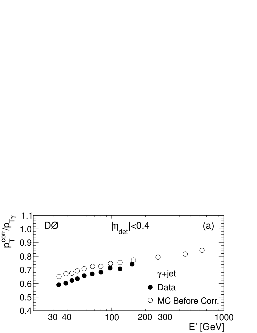
(a)

(b)

(c)

(d)

Figure 33: Tuning of single-particle responses (Sec. 14.1.2) using the ratio ${p^{\textnormal{corr}}_{\textnormal{T}}}/{p^{\textnormal{}}_{\textnormal{T{$\gamma$}}}}$ as a function of $E^{\prime}$ (Eq. 14) for jets with ${\left|{{\eta_{\textnormal{det}}^{\textnormal{}}}}\right|}<0.4$ in a high-purity ${\gamma}+\textnormal{jet}$ sample, LABEL:sub@fig:fdc:data_closure1_gamjet_default before the MC response correction and LABEL:sub@fig:fdc:data_closure1_gamjet_newTune after the correction. Plots LABEL:sub@fig:fdc:data_closure1_antgamjet_default and LABEL:sub@fig:fdc:data_closure1_antgamjet_newTune show similar results for the dijet events.

14.2 Results

The tuning of parameters $A$, $B$, and $C$ is performed using a fit, which is performed simultaneously for the ${\gamma}+\textnormal{jet}$ and dijet samples. The procedure is applied for four different $\left|{{\eta_{\textnormal{det}}^{\textnormal{}}}}\right|$ regions of the detector. Figure 33 shows the result of the tuning for jets with ${\left|{{\eta_{\textnormal{det}}^{\textnormal{}}}}\right|}<0.4$ in samples dominated by ${\gamma}+\textnormal{jet}$ and dijet events. The ${p^{\textnormal{corr}}_{\textnormal{T}}}/{p^{\textnormal{}}_{\textnormal{T{$\gamma$}}}}$ ratios are shown before and after MC tuning. Good agreement between MC and data is obtained.

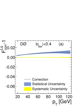
(a)

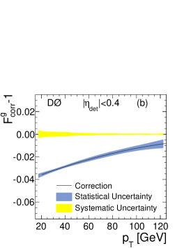
(b)

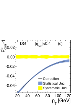
(c)

Figure 34: (color online) Correction factor $F_{\textnormal{corr}}$ derived using tuned MC single-particle responses for central jets (${\left|{{\eta_{\textnormal{det}}^{\textnormal{}}}}\right|}<0.4$) and different jet flavors, shown separately for jets from LABEL:sub@fig:fdc:final1_light light quarks ($u$, $d$, $s$, $c$), LABEL:sub@fig:fdc:final1_gluon gluons, and LABEL:sub@fig:fdc:final1_b $b$ quarks. The bands represent the statistical and systematic uncertainties.

The resulting relative jet energy correction factors $F_{\textnormal{corr}}$ for different jet flavors (light quark, gluon, and bottom quark) are shown in Fig. 34. The relative correction required for the light quarks is 1%, but it is significantly larger for gluon and $b$-quark jets, where energies are undercorrected by a few percent, especially at low $p^{\textnormal{}}_{\textnormal{T}}$.

The dominant contribution to the uncertainty is obtained by propagating the fit errors on the three parameters $A$, $B$, and $C$ as estimated by the covariance matrix and is typically smaller than 0.5%. The assumption that the $\gamma$ and $e^{\pm}$ responses are well simulated in MC needs to be verified. The $\gamma$ and $e^{\pm}$ responses are varied according to the accuracy of their energy scale calibration (0.6% and 0.3% respectively), and the effect is found to be negligible.

15 Jet-$p^{\textnormal{}}_{\textnormal{T}}$ shifting and smearing in Monte Carlo

15.1 Introduction

In many physics analyses results are derived from a comparison between data and MC simulations. Given the limitations of MC simulation (e.g., in the modeling of the parton showering and approximations in the modeling of the D0 detector), it is necessary to modify the standard simulation in order to match the performance observed in data. This is especially true for jets. A method has been developed to correct the simulated jets by the residual data/MC difference in energy scale, resolution, and reconstruction efficiency, known as Jet Shifting Smearing and Removal (JSSR) method.

To derive these JSSR corrections, we select $Z+\textnormal{jet}$ events in data and MC (see Sec. 6). The observable used in this study is the transverse momentum imbalance in a two-body process, given by:

$${\Delta S_{\textnormal{}}}=\frac{{p^{\textnormal{}}_{\textnormal{T}}}-{p^{Z\textnormal{}}_{\textnormal{T}}}}{{p^{Z\textnormal{}}_{\textnormal{T}}}},$$ (54)

where $p^{Z\textnormal{}}_{\textnormal{T}}$ and $p^{\textnormal{}}_{\textnormal{T}}$ are the $Z$-boson and jet transverse momenta.

In our data/MC consistency checks (Sec. 13) we confirmed that jet energies in data and MC are intercalibrated, i.e., $E^{\textnormal{ptcl}}_{\textnormal{}}$ is reproduced within the estimated uncertainties in ${\gamma}+\textnormal{jet}$ events. Therefore, the value of the $\Delta S_{\textnormal{}}$ variable is sensitive to differences in the flavor compositions of jets balancing the $Z$ boson versus those balancing the photon. Since at small photon $p^{\textnormal{}}_{\textnormal{T}}$ the jets produced in ${\gamma}+\textnormal{jet}$ events are mostly “quark” jets, $qg\to q{\gamma}$ (see Fig. 40 in Sec. 16), we calibrate mostly quark jets when applying the MPF procedure, and the $\Delta S_{\textnormal{}}$ for calibrated quark jets should be consistent between data and MC, yielding ${\Delta S_{\textnormal{}}}_{\textnormal{data}}^{q}-{\Delta S_{\textnormal{}}}_{\textnormal{MC}}^{q}=0$. This is also confirmed by the small residual shift, $(+1.3\pm 0.8)\%$, observed by constraining the $W$ boson mass reconstructed from decays into two quark jets in Ref. [7]. However, as shown in Fig. 35, the flavor composition predicted by the pythia simulation in $Z+\textnormal{jet}$ events is different than in ${\gamma}+\textnormal{jet}$, and a relative data/MC shift in $\Delta S_{\textnormal{}}$ is observed in $Z+\textnormal{jet}$ events which is related to the larger fraction of gluon jets in the final state. At high energies the jet response for both quark and gluon jets increases, and jet energy scale corrections become smaller (see Fig. 41, Sec. 16). Also, the jet flavor compositions in ${\gamma}+\textnormal{jet}$ and $Z+\textnormal{jet}$ events converge. Thus, the calibrated $\Delta S_{\textnormal{}}$ shift is expected to vanish at large jet energies in $Z+\textnormal{jet}$ events.

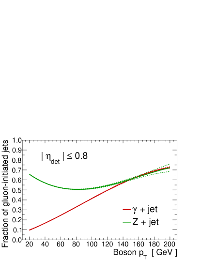
Figure 35: (color online) Fraction of gluon-initiated jets in $Z+\textnormal{jet}$ and ${\gamma}+\textnormal{jet}$ events with the jet in the central calorimeter according to pythia simulation.

15.2 Event selection

This study is performed using the $Z+\textnormal{jet}$ sample with $Z$ bosons decaying into a $\mu^{+}\mu^{-}$ pair. The muon momentum is calibrated with an accuracy of about 0.3% [18]. The selected events are required to contain only one jet and two muons. The two muons are required to have ${p^{\textnormal{$\mu$}}_{\textnormal{T}}}\geq{15\mskip 4.0mu plus 2.0mu minus 2.5mu\textnormal{GeV}}$, $\left|{\eta^{\mu}}\right|<2.0$, and the dimuon invariant mass is required to be in the range $80<M_{\mu\mu}<{110\mskip 4.0mu plus 2.0mu minus 2.5mu\textnormal{$\textnormal{GeV}$}}$ . The jet should be within ${\left|{{\eta_{\textnormal{det}}^{\textnormal{}}}}\right|}<2.4$. Finally, the $Z$ boson must be back to back with respect to the jet in the transverse plane: $\Delta{\phi}(Z,\textnormal{jet})\geq{2.8\mskip 4.0mu plus 2.0mu minus 2.5mu\textnormal{rad}}$. The data and MC are first calibrated with the energy scale correction as described in the previous sections, including the single-particle response correction (Sec. 14) for MC jets. In both data and MC, the muon momentum is calibrated using $Z\to\mu\mu$ events. The muon energy resolution in MC is also tuned to data using the reconstructed width of the $Z\to\mu\mu$ mass peak.

15.3 Procedure

The $Z+\textnormal{jet}$ events are split into different samples with similar $p^{Z\textnormal{}}_{\textnormal{T}}$, covering the range $10\leq{p^{Z\textnormal{}}_{\textnormal{T}}}\leq{250\mskip 4.0mu plus 2.0mu minus 2.5mu\textnormal{GeV}}$. For each subsample, a $\Delta S_{\textnormal{}}$ (Eq. 54) distribution is obtained. Figure 36 shows that $\Delta S$ for ${p^{Z\textnormal{}}_{\textnormal{T}}}>{40\mskip 4.0mu plus 2.0mu minus 2.5mu\textnormal{$\textnormal{GeV}$}}$ is well described by a Gaussian distribution, as expected due to the $p^{\textnormal{}}_{\textnormal{T}}$ imbalance and reconstruction resolution of both jet and $Z$ boson. However, as the $p^{Z\textnormal{}}_{\textnormal{T}}$ decreases, this simple description fails because of the jet $p^{\textnormal{}}_{\textnormal{T}}$ reconstruction threshold used in the jet finding algorithm (${p^{\textnormal{meas}}_{\textnormal{T}}}>{6\mskip 4.0mu plus 2.0mu minus 2.5mu\textnormal{$\textnormal{GeV}$}}$, see Sec. 3.4). Therefore, in the more general case, $\Delta S_{\textnormal{}}$ should be described by a function composed of a Gaussian distribution, combined with an Error Function ($\operatorname{erf}$) used to represent the jet $p^{\textnormal{}}_{\textnormal{T}}$ threshold effect:

$$A\,\exp\left[{-\frac{\left({{\Delta S_{\textnormal{}}}-\left<{{\Delta S_{\textnormal{}}}}\right>}\right)^{2}}{2\,\sigma_{{\Delta S_{\textnormal{}}}}^{2}}}\right]\left[{1+\operatorname{erf}\left(\frac{{\Delta S_{\textnormal{}}}-T}{\sqrt{2}\,\sigma_{T}}\right)}\right],$$ (55)

with five free parameters: the relative average shift of jet $p^{\textnormal{}}_{\textnormal{T}}$ with respect to $p^{Z\textnormal{}}_{\textnormal{T}}$, $\left<{{\Delta S_{\textnormal{}}}}\right>$, the resolution smearing of the jet $p^{\textnormal{}}_{\textnormal{T}}$, $\sigma_{{\Delta S_{\textnormal{}}}}$, the parameters of the Error Function, $T$ and $\sigma_{T}$ (used to model the removal of low $p^{\textnormal{}}_{\textnormal{T}}$ jets), and a normalization factor, $A$. The muon resolution is negligible compared to jet resolution.

The shifting, smearing, and removal parameters are derived independently for data and MC samples in two steps, described below, and are combined into the final correction.

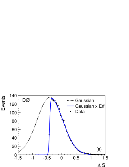
(a)

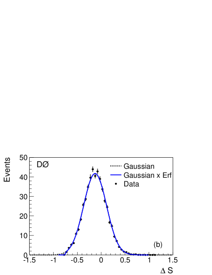
(b)

Figure 36: The $\Delta S_{\textnormal{}}$ distribution in the MC sample, for $p^{Z\textnormal{}}_{\textnormal{T}}$ in the ranges LABEL:sub@fig:dS_19_22 $19-22\mskip 4.0mu plus 2.0mu minus 2.5mu\textnormal{$\textnormal{GeV}$}$ and LABEL:sub@fig:dS_45_50 $45-50\mskip 4.0mu plus 2.0mu minus 2.5mu\textnormal{$\textnormal{GeV}$}$. The solid line shows the best fitting function according to Eq. 54, while the dashed line shows only its Gaussian component. The threshold effect is negligible for $p^{Z\textnormal{}}_{\textnormal{T}}$ larger than $40\mskip 4.0mu plus 2.0mu minus 2.5mu\textnormal{GeV}$.

The corrections, for application in MC events, are extracted independently for jets falling into three distinct detector regions: ${\left|{{\eta_{\textnormal{det}}^{\textnormal{}}}}\right|}<0.8$, $0.8\leq{\left|{{\eta_{\textnormal{det}}^{\textnormal{}}}}\right|}<1.6$ and ${\left|{{\eta_{\textnormal{det}}^{\textnormal{}}}}\right|}\geq 1.6$.

15.3.1 Jet reconstruction threshold

The five parameters of Eq. 55 are first obtained from the fit to the $\Delta S_{\textnormal{}}$ distribution in data and MC, for each $\left|{{\eta_{\textnormal{det}}^{\textnormal{}}}}\right|$ and $p^{Z\textnormal{}}_{\textnormal{T}}$ range. The threshold parameters $T$ and $\sigma_{T}$ are found to be almost independent of $p^{Z\textnormal{}}_{\textnormal{T}}$ (Fig. 37) and $\eta$ region, with a mean value $T$ of about $12\mskip 4.0mu plus 2.0mu minus 2.5mu\textnormal{$\textnormal{GeV}$}$ and standard deviation $\sigma_{T}$ of about $1\mskip 4.0mu plus 2.0mu minus 2.5mu\textnormal{$\textnormal{GeV}$}$. Based on this, the value of $15\mskip 4.0mu plus 2.0mu minus 2.5mu\textnormal{$\textnormal{GeV}$}$ ($\approx\!3\,\sigma_{T}$ above $T$) is recommended as the $p^{\textnormal{}}_{\textnormal{T}}$ threshold for jet selection in physics analyses. This ensures close to 100% jet reconstruction efficiency for both data and MC.

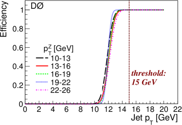
Figure 37: (color online) The jet reconstruction efficiency turn-on curve as function of the jet $p^{\textnormal{}}_{\textnormal{T}}$ for different $p^{Z\textnormal{}}_{\textnormal{T}}$ ranges of the MC sample. The efficiency curve for data is very similar. The physics analysis selection threshold of $15\mskip 4.0mu plus 2.0mu minus 2.5mu\textnormal{$\textnormal{GeV}$}$ is also shown.

15.3.2 Relative energy scale and resolution

Due to the universality of the threshold $T$, the second step of the procedure can be simplified by fixing the threshold to the value of $12\mskip 4.0mu plus 2.0mu minus 2.5mu\textnormal{$\textnormal{GeV}$}$. In this step, a fit is performed to find the values of the other four parameters that best describe the $\Delta S_{\textnormal{}}$ distribution in each $p^{Z\textnormal{}}_{\textnormal{T}}$ range. In regions with ${p^{Z\textnormal{}}_{\textnormal{T}}}>{40\mskip 4.0mu plus 2.0mu minus 2.5mu\textnormal{$\textnormal{GeV}$}}$, where the threshold has no effect, a simplified distribution made of a single Gaussian is employed in place of Eq. 55.

The difference between data and MC scale shifts $\left<{{\Delta S_{\textnormal{data}}}}\right>-\left<{{\Delta S_{\textnormal{MC}}}}\right>$ is used for the relative correction of MC jet $p^{\textnormal{}}_{\textnormal{T}}$. This is the “shifting” part of the correction. Figure 38 shows this correction for jets in the central region of the calorimeter. In general, the residual shifting is small ($\approx 1\%$) for high energies, while it becomes relevant for low energies.

The procedure of optimization of the parameters in Eq. 55 is unstable for small $p^{Z\textnormal{}}_{\textnormal{T}}$, where the threshold effect is so dominant that the parameters of the shape must be inferred from just the tail of the Gaussian distribution of $\Delta S_{\textnormal{}}$, as shown in 36a. Therefore to cover the region ${p^{Z\textnormal{}}_{\textnormal{T}}}<{20\mskip 4.0mu plus 2.0mu minus 2.5mu\textnormal{$\textnormal{GeV}$}}$, an extrapolation is preferred to the direct measurement.

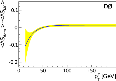
Figure 38: (color online) Residual jet energy shifting as a function of $\left<{{p^{Z\textnormal{}}_{\textnormal{T}}}}\right>$ for central jets (${\left|{{\eta_{\textnormal{det}}^{\textnormal{}}}}\right|}<0.8$). The yellow band shows its statistical uncertainty.

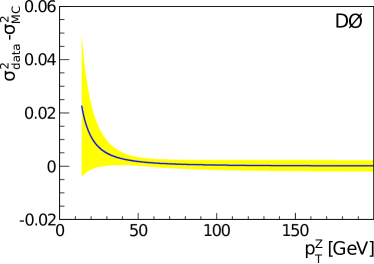
Figure 39: (color online) Jet resolution correction as a function of $\left<{{p^{Z\textnormal{}}_{\textnormal{T}}}}\right>$ for central jets (${\left|{{\eta_{\textnormal{det}}^{\textnormal{}}}}\right|}<0.8$). The yellow band shows the statistical uncertainty.

When the residual energy shifts are extracted, the same procedure also provides the resolution parameter $\sigma_{{\Delta S_{\textnormal{}}}}$. The quadratic difference in resolution between data and MC, $\sigma^{2}_{\textnormal{data}}-\sigma^{2}_{\textnormal{MC}}$, is used to “smear” the jet $p^{\textnormal{}}_{\textnormal{T}}$ in MC simulation. Figure 39 shows that the resolutions for central jets are similar in data and MC.

15.3.3 Application of the correction

The JSSR corrections are applied to all MC jets. Since the corrections were derived as a function of $p^{Z\textnormal{}}_{\textnormal{T}}$, but need to be applied to jets as a function of jet $p^{\textnormal{}}_{\textnormal{T}}$, a mapping is used between the average jet $p^{\textnormal{}}_{\textnormal{T}}$ and $p^{Z\textnormal{}}_{\textnormal{T}}$. This mapping is mostly linear, with a residual non-linearity in the low $p^{Z\textnormal{}}_{\textnormal{T}}$ regions due to the jet reconstruction threshold discussed in Sec. 15.3.1.

The JSSR corrections are applied as follows. First, the energy of the jets in MC is smeared according to $\sigma^{2}_{\textnormal{corr}}=\sigma^{2}_{\textnormal{data}}-\sigma^{2}_{\textnormal{MC}}$. If the fitted $\sigma^{2}_{\textnormal{corr}}$ value is negative, the correction is not applied. Secondly, the jet $p^{\textnormal{}}_{\textnormal{T}}$ is shifted by the amount corresponding to $\left<{{\Delta S_{\textnormal{}}}_{\textnormal{data}}}\right>-\left<{{\Delta S_{\textnormal{}}}_{\textnormal{MC}}}\right>$. Finally, if the resulting jet $p^{\textnormal{}}_{\textnormal{T}}$ is below $15\mskip 4.0mu plus 2.0mu minus 2.5mu\textnormal{$\textnormal{GeV}$}$, the jet is removed from the list of jets in the event.

The JSSR corrections are applied in addition to all the jet energy scale corrections described in Sec. 4, which are derived with ${\gamma}+\textnormal{jet}$ events. The single-particle response correction (Sec. 14) applied jet-by-jet separately for different jet flavors (see Fig. 34), significantly reduces variation in jet $p^{\textnormal{}}_{\textnormal{T}}$ scale and resolution between data and MC, with a negligible residual difference for $p^{\textnormal{}}_{\textnormal{T}}$ resolution and reduced relative $p^{\textnormal{}}_{\textnormal{T}}$ shifting. Instrumental and other detector effects in the ICD region affect the agreement of the MC description with data resulting in larger systematic uncertainties in this region.

15.4 Uncertainties

As described in Sec. 15.3.2, the basic procedure to derive shifting and smearing corrections is the same. When the fit is performed for data and MC, it delivers the best-fit parameter values and the covariance matrix. The uncertainty on the final correction is obtained by error propagation, combining the two uncertainties from data and MC as independent. The bands in Figs. 38 and 39 represent the uncertainty on the correction. Both for shifting and smearing in the high $p^{Z\textnormal{}}_{\textnormal{T}}$ regions, the uncertainty is of the order of 0.5%, while for ${p^{Z\textnormal{}}_{\textnormal{T}}}<{20\mskip 4.0mu plus 2.0mu minus 2.5mu\textnormal{$\textnormal{GeV}$}}$ it increases up to 4%–7% for the jet $p^{\textnormal{}}_{\textnormal{T}}$ shifting and 2%–3% for the $p^{\textnormal{}}_{\textnormal{T}}$ smearing.

16 Dijet-specific corrections

The jet energy calibration corrections derived so far are designed to correct the energy of jets with a flavor composition similar to that in the ${\gamma}+\textnormal{jet}$ sample. Event samples chosen for particular analyses may differ substantially from this case. For example, Figure 40 shows the fraction of gluon-initiated jets in the CC region for ${\gamma}+\textnormal{jet}$ and dijet events simulated with pythia. Furthermore, these corrections are not guaranteed to properly calibrate to the particle level all the jet four-momentum components. These caveats do not represent significant limitations for physics measurements relying on the comparison of observables between data and MC, which benefit from JSSR corrections. Rather than on the absolute energy scale calibration, these measurements depend on the relative intercalibration of MC and data (Secs. 14 and 15).

In contrast, most of the QCD physics program is based on the comparison of observables in data, corrected to the particle level, with theoretical predictions. These measurements depend on the absolute energy calibration of jets in data. As discussed previously, the different flavor composition of jets in dijet events as compared to ${\gamma}+\textnormal{jet}$ production requires a dedicated jet energy calibration to be derived for this sample. Furthermore, many of the observables considered in dijet QCD measurements (jet $p^{\textnormal{}}_{\textnormal{T}}$, $\eta$, dijet mass) involve components of the four-momentum other than the energy that are also required to be properly calibrated to the particle level (see, for example, Refs. [3, 4, 5]).

This section outlines the calibration strategy of the jet four-momentum in the dijet sample. These corrections are determined only for ${\mathcal{R}_{\textnormal{cone}}}=0.7$ jets, used for the QCD jet measurements at D0. A more complete description can be found in Ref. [4].

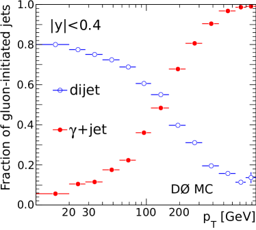
Figure 40: (color online) Fraction of gluon-initiated jets in ${\gamma}+\textnormal{jet}$ and dijet events in the central calorimeter.

16.1 Jet energy calibration

To understand what modifications are required to properly calibrate jet energies in the dijet sample, it is useful to start from the expression of the corrected energy in case of the ${\gamma}+\textnormal{jet}$ sample, making explicit the different subcorrections. Given a jet with detector pseudorapidity $\eta_{\textnormal{det}}^{\textnormal{}}$, the corrected jet energy, following Eqs. 9 and 22, is given by:

$${E^{\textnormal{corr}}_{\textnormal{}}}=\frac{{E^{\textnormal{meas}}_{\textnormal{}}}-\hat{E}_{\textnormal{O}}}{{R_{\textnormal{MPF,CC}}^{\textnormal{{${\gamma}+\textnormal{jet}$}}}}\,{F_{\eta}^{\textnormal{{${\gamma}+\textnormal{jet}$}}}}\,{k_{\textnormal{R}}^{\textnormal{topo,{${\gamma}+\textnormal{jet}$}}}}\,S^{\textnormal{{${\gamma}+\textnormal{jet}$}}}}\cdot\frac{{{k_{\textnormal{O}}^{\textnormal{ZS}}}}}{{{k_{\textnormal{R}}^{\textnormal{ZS}}}}}$$ (56)

where all subcorrections which are expected to be sample-dependent are denoted with the superscript “${\gamma}+\textnormal{jet}$”.

To calibrate the jet energy in the QCD dijet sample, it is necessary to redetermine every sample-dependent subcorrection above. The relative MPF response correction (${F_{\eta}^{\textnormal{{$\textnormal{dijet}$}}}}$) was already determined in Sec. 9 and is therefore available. It is possible to estimate the showering correction directly from dijet data following a similar approach to the one used in Sec. 11. However, the absolute MPF response correction can not be estimated from dijet data. By taking into account the nature of each of the subcorrections, it can be demonstrated that the energy for jets from QCD dijet events can be properly calibrated using the following modified formula:

$${E^{\textnormal{corr}}_{\textnormal{}}}=\frac{{E^{\textnormal{meas}}_{\textnormal{}}}-\hat{E}_{\textnormal{O}}}{{R_{\textnormal{MPF,CC}}^{\textnormal{{${\gamma}+\textnormal{jet}$}}}}\,{F_{\eta}^{\textnormal{{$\textnormal{dijet}$}}}}\,{k_{\textnormal{R}}^{\textnormal{topo,{${\gamma}+\textnormal{jet}$}}}}\,\Delta_{R}\,S^{\textnormal{{$\textnormal{dijet}$}}}}\cdot\frac{{{k_{\textnormal{O}}^{\textnormal{ZS}}}}}{{{k_{\textnormal{R}}^{\textnormal{ZS}}}}}$$ (57)

where the main difference is the replacement of $S^{{{\gamma}+\textnormal{jet}}}$ with $S^{{\textnormal{dijet}}}$ and the addition of the correction factor $\Delta_{R}={R_{\textnormal{MPF,CC}}^{\textnormal{{${\gamma}+\textnormal{jet}$}}}}/{R_{\textnormal{MPF,CC}}^{\textnormal{{$\textnormal{dijet}$}}}}$, defined as the ratio of true jet responses in the ${\left|{{\eta_{\textnormal{det}}^{\textnormal{}}}}\right|}<0.4$ region between ${\gamma}+\textnormal{jet}$ and dijet events.

The two additional corrections are evaluated in MC, for both data and MC jet energy calibration. In the case of $S^{{\textnormal{dijet}}}$, this is justified by the consistency of the direct measurements of $S^{{{\gamma}+\textnormal{jet}}}$ in MC and in data (see Fig. 23). Also, the MC simulation shows that the different jet flavor composition between dijet and ${\gamma}+\textnormal{jet}$ events results in a very small difference in the true showering correction, typically less than $1\%$. Nevertheless, this correction is explicitly included.

In contrast, the MC simulation predicts a significant difference in true jet response for central jets between ${\gamma}+\textnormal{jet}$ and dijet events, as shown in Fig. 41. Their ratio is estimated using MC with a tuned single-particle response (Sec. 14). The same ratio is also used for data.

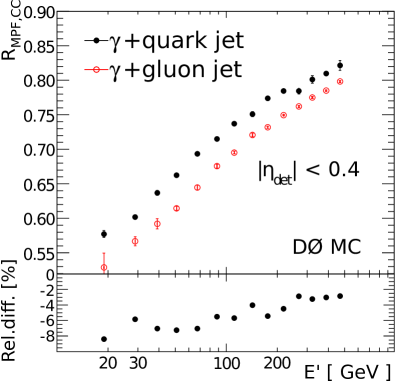
Figure 41: Quark- and gluon-initiated jet responses and their relative differences for jets with ${\left|{{\eta_{\textnormal{det}}^{\textnormal{}}}}\right|}<0.4$ jets as a function of $E^{\prime}$.

16.2 Jet $p^{\textnormal{}}_{\textnormal{T}}$ calibration

The procedure for the calibration of jet $p^{\textnormal{}}_{\textnormal{T}}$ relies on the available subcorrections from energy calibration, and the corrected jet $p^{\textnormal{}}_{\textnormal{T}}$ is estimated from the measured one, $p^{\textnormal{meas}}_{\textnormal{T}}$, according to the following expression:

$${p^{\textnormal{corr}}_{\textnormal{T}}}=\frac{{p^{\textnormal{meas}}_{\textnormal{T}}}-p_{\textnormal{T,O}}}{{R_{\textnormal{MPF,CC}}^{\textnormal{{${\gamma}+\textnormal{jet}$}}}}\,{F_{\eta}^{\textnormal{{$\textnormal{dijet}$}}}}\,{k_{\textnormal{R},{p^{\textnormal{}}_{\textnormal{T}}}}^{\textnormal{topo,{${\gamma}+\textnormal{jet}$}}}}\,\Delta_{R}\,{S_{{p^{\textnormal{}}_{\textnormal{T}}}}^{\textnormal{{$\textnormal{dijet}$}}}}}\cdot\frac{{k_{\textnormal{O},{p^{\textnormal{}}_{\textnormal{T}}}}^{\textnormal{ZS}}}}{{{k_{\textnormal{R}}^{\textnormal{ZS}}}}}$$ (58)

where $p_{\textnormal{T,O}}$ stands for the offset $p^{\textnormal{}}_{\textnormal{T}}$ correction, $k_{\textnormal{O},{p^{\textnormal{}}_{\textnormal{T}}}}^{\textnormal{ZS}}$ is the zero-suppression bias correction to the estimated offset $p^{\textnormal{}}_{\textnormal{T}}$, $k_{\textnormal{R},{p^{\textnormal{}}_{\textnormal{T}}}}^{\textnormal{topo,{${\gamma}+\textnormal{jet}$}}}$ is the $p^{\textnormal{}}_{\textnormal{T}}$-based topology bias correction to MPF response and $S_{{p^{\textnormal{}}_{\textnormal{T}}}}^{\textnormal{{$\textnormal{dijet}$}}}$ is the true showering correction to $p^{\textnormal{}}_{\textnormal{T}}$.

Since the offset correction has been explicitly measured only for energy and not for $p^{\textnormal{}}_{\textnormal{T}}$, the following approximation is used:

$$\left({{p^{\textnormal{meas}}_{\textnormal{T}}}-p_{\textnormal{T,O}}}\right){k_{\textnormal{O},{p^{\textnormal{}}_{\textnormal{T}}}}^{\textnormal{ZS}}}\simeq\frac{{p^{\textnormal{meas}}_{\textnormal{T}}}}{{E^{\textnormal{meas}}_{\textnormal{}}}}\left({{E^{\textnormal{meas}}_{\textnormal{}}}-\hat{E}_{\textnormal{O}}}\right){{k_{\textnormal{O}}^{\textnormal{ZS}}}},$$ (59)

which is expected to be sufficiently accurate in the kinematic range of interest of QCD measurements (typically ${p^{\textnormal{corr}}_{\textnormal{T}}}>{40\mskip 4.0mu plus 2.0mu minus 2.5mu\textnormal{$\textnormal{GeV}$}}$).

Similarly to Eq. 19, the $p^{\textnormal{}}_{\textnormal{T}}$-based topology bias correction to MPF response is defined as:

$${k_{\textnormal{R},{p^{\textnormal{}}_{\textnormal{T}}}}^{\textnormal{topo,{${\gamma}+\textnormal{jet}$}}}}=\frac{{R_{{p^{\textnormal{}}_{\textnormal{T}}}}^{\textnormal{{${\gamma}+\textnormal{jet}$}}}}}{{R_{\textnormal{MPF}}^{\textnormal{{${\gamma}+\textnormal{jet}$},noZB}}}},$$ (60)

where $R_{{p^{\textnormal{}}_{\textnormal{T}}}}^{\textnormal{{${\gamma}+\textnormal{jet}$}}}$ is the $p^{\textnormal{}}_{\textnormal{T}}$-based true jet response (cf. Eq. 6):

$${R_{{p^{\textnormal{}}_{\textnormal{T}}}}^{\textnormal{{${\gamma}+\textnormal{jet}$}}}}=\frac{\left\|{\sum_{i\in\textnormal{ptcljet}}\vec{p}^{\,\textnormal{meas}}_{\textnormal{T$i$}}}\right\|}{{p^{\textnormal{ptcl}}_{\textnormal{T}}}}.$$ (61)

This correction is closer to unity than the one for energy, being typically 1.0%–2.5% for ${\left|{{\eta_{\textnormal{det}}^{\textnormal{}}}}\right|}<2.5$. This indicates that the MPF method is more suitable for $p^{\textnormal{}}_{\textnormal{T}}$ calibration than for energy calibration.

Finally, the true showering correction to $p^{\textnormal{}}_{\textnormal{T}}$ is defined similarly to the (energy-based) true showering correction (see Eq. 7):

$${S_{{p^{\textnormal{}}_{\textnormal{T}}}}^{\textnormal{}}}=\frac{\left\|{\sum_{i\in\textnormal{ptcljet}}\vec{p}^{\,\textnormal{meas}}_{\textnormal{T$i$}}f_{i}+\sum_{i\notin\textnormal{ptcljet}}\vec{p}^{\,\textnormal{meas}}_{\textnormal{T$i$}}f_{i}}\right\|}{\left\|{\sum_{i\in\textnormal{ptcljet}}\vec{p}^{\,\textnormal{meas}}_{\textnormal{T$i$}}}\right\|}.$$ (62)

As expected, the net $p^{\textnormal{}}_{\textnormal{T}}$ flow through the jet cone boundary is smaller than the net energy flow, with $S_{{p^{\textnormal{}}_{\textnormal{T}}}}^{\textnormal{}}$ values of $-3\%$ to $1\%$ for ${\left|{{\eta_{\textnormal{det}}^{\textnormal{}}}}\right|}<2.5$.

16.3 Four-momentum correction

The MC simulation shows that the reconstructed jet rapidity is generally biased towards the central calorimeter with respect to the true (particle level) jet rapidity, with the largest deviations observed in the ICR region. This bias is attributed to detector effects in the ICR in addition to the jet cone algorithm itself. The absolute effect on the inclusive jet measurement is small compared to the effect of jet $p^{\textnormal{}}_{\textnormal{T}}$ calibration, being the largest (4%) at ${\left|{{\eta_{\textnormal{det}}^{\textnormal{}}}}\right|}\simeq 1.5$ [4]. The correction $\Delta y$ for this bias is parametrized as a function of $\eta$ and applied to the reconstructed jets:

$$y^{\textnormal{corr}}=y^{\textnormal{meas}}-\Delta y.$$ (63)

The calibrated jet four-momentum $p^{\mu,\textnormal{corr}}$ is given by:

$$p^{\mu,\textnormal{corr}}=\left({{E^{\textnormal{corr}}_{\textnormal{}}},\,{p^{\textnormal{corr}}_{\textnormal{T}}}\cos{\phi}^{\textnormal{corr}},\,{p^{\textnormal{corr}}_{\textnormal{T}}}\sin{\phi}^{\textnormal{corr}},\,p_{z}^{\textnormal{corr}}}\right),$$ (64)

where $E^{\textnormal{corr}}_{\textnormal{}}$ and $p^{\textnormal{corr}}_{\textnormal{T}}$ are defined, respectively, in Eqs. 57 and 58. The measured jet azimuthal angle is assumed to be unbiased, and thus ${\phi}^{\textnormal{corr}}={\phi}^{\textnormal{meas}}$. Finally, given the calibrated jet energy and rapidity (Eqs. 57 and 63):

$$p_{z}^{\textnormal{corr}}={E^{\textnormal{corr}}_{\textnormal{}}}\ \frac{\exp\left(2\,y^{\textnormal{corr}}\right)-1}{\exp\left(2\,y^{\textnormal{corr}}\right)+1}\ .$$ (65)

17 Correlations between jets

Knowledge of the correlation of the JES uncertainties between jets at different energies and pseudorapidities is important for a proper comparison of measured quantities with theoretical predictions. This information is needed, for example, in the global fits of parton distribution functions. Correlations also play an important role in various new physics searches and they have a direct impact on the expected sensitivity.

Determination of these correlations is a more complex task than determining the individual uncertainties. At the same time, it facilitates the calculation of the correlations in physics analyses. The method of deriving the correlations is introduced in Sec. 17.1, followed by the presentation and discussion of the results.

17.1 Method

To evaluate correlations, the total uncertainty is split into the individual components of photon energy scale uncertainty, statistical uncertainty of the central jet response fit, and other components. These individual components will be called “uncertainty sources”.

To simplify the description, each source is assumed to be independent from the others. This is true in most cases. For example, the photon energy scale uncertainty has no connection to the showering systematics. Each individual uncertainty source is assigned a function $\Delta_{\textnormal{s}}$ describing the relative change in jet energy correction that corresponds to a “$1\sigma$” modification of source $s$ (where $\sigma$ is a standard deviation). These functions depend on jet energy and pseudorapidity. While in most cases this is straightforward, a few exceptions are discussed later, for example, the fit uncertainties, which are driven by the covariance matrix of the fit parameters and therefore can not be considered independent.

The functions ${\Delta_{\textnormal{s}}}\left(E,\eta\right)$ can be used to calculate correlations in jet energy uncertainties across different regions of jet energies, $E$, and pseudorapidities, $\eta$. They can also be used directly to evaluate jet energy scale correlations in an analysis.

17.1.1 Treatment of systematic uncertainties

In most cases, the sources of systematic uncertainties can be treated as uncorrelated with each other. They are treated as fully correlated in jet energy and $\eta$, which means that their effect on the jet energy scale can be described by the ${\Delta_{\textnormal{s}}}\left(E,\eta\right)$ functions.

Typically all the required information is directly available from the studies of a given source of systematics. For example, a $0.5\%$ shift in electron energy scale, one of the dominant uncertainties for central jets, directly introduces a $0.5\%$ shift in jet energy scale for all jet energies and angles, i.e., ${\Delta_{\textnormal{s}}}\left(E,\eta\right)=0.005$ for this particular source.

However, in some cases, such as for uncertainties in modeling of soft underlying physics, the uncertainty is determined as an envelope covering various options of MC generators and their parameters. Different MC models give different correlations across jet energies and directions. Since such sources do not give significant contributions to the final error, an envelope function is assigned to ${\Delta_{\textnormal{s}}}\left(E,\eta\right)$ to simplify the model.

17.1.2 Treatment of statistical uncertainties from the response fit

Special treatment is needed for the error of the absolute response (Sec. 8) fit where correlations across jet energies are introduced. In general, these correlations are fully described by the error matrix of the fit. To treat them properly in the framework of independent sources, the error matrix is diagonalized by appropriate linear transformation in the space of fit parameters. The parametric response fit is thus transformed into three independent uncertainty sources and error functions ${\Delta_{\textnormal{s}}}$ that correspond to the modification in jet response due to one standard deviation change in the respective transformed fit parameters.

17.1.3 Treatment of correlations across $\eta$

The same treatment as for the jet absolute response fit can be applied to the “global fit” of the relative $\eta$-dependent correction (Sec. 9.1.4). However, this treatment would be unpractical, since the global fit contains 57 parameters, requiring the introduction of as many sources of uncertainties.

Instead, the calorimeter is divided into seven regions of detector pseudorapidity: ${\eta_{\textnormal{det}}^{\textnormal{}}}<-2.0$, $-2.0\leq{\eta_{\textnormal{det}}^{\textnormal{}}}<-1.6$, $-1.6\leq{\eta_{\textnormal{det}}^{\textnormal{}}}<-1.2$, $-1.2\leq{\eta_{\textnormal{det}}^{\textnormal{}}}\leq 1.2$, $1.2<{\eta_{\textnormal{det}}^{\textnormal{}}}\leq 1.6$, $1.6<{\eta_{\textnormal{det}}^{\textnormal{}}}\leq 2.0$, and ${\eta_{\textnormal{det}}^{\textnormal{}}}>2.0$. Within these regions, jets are considered fully correlated in $\eta$. This partition is motivated by the analysis of the correlations in pseudorapidity from the global fit of $\eta$-dependent corrections for a set of values of jet $p^{\textnormal{}}_{\textnormal{T}}$ (Fig. 42).

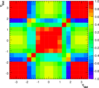
Figure 42: (color online) Correlations between two jets at different pseudorapidities for ${p^{\textnormal{}}_{\textnormal{T}}}={50\mskip 4.0mu plus 2.0mu minus 2.5mu\textnormal{GeV}}$, from the global fit to the $\eta$-dependent corrections for ${\mathcal{R}_{\textnormal{cone}}}=0.7$ jets in data.

One uncertainty source is assigned to each of the seven calorimeter regions. Each error function ${\Delta_{\textnormal{s}}}$ is defined to be equal to the error of the global fit for jets within its particular calorimeter region, and equal to zero outside. To avoid abrupt changes in the correlations at the boundaries of the calorimeter regions, smoothly falling functions are used around their edges.

Finally, all sources are decomposed into uncorrelated ones by diagonalizing the correlation matrix.

17.2 Results

The jet energy scale uncertainty for ${\gamma}+\textnormal{jet}$ events is split into a total of 48 independent sources (54 for the dijet events). This number is still large, and further simplification is possible by the identification of the most important sources and the merging of the remaining ones into a single residual source. This approach is applied, for example, in the inclusive jet cross section measurement [3, 4].

The method of calculating the correlations for an arbitrary observable described in Sec. 17.1 can be applied to calculate the correlations between the jet energy scale corrections for two jets at different energies and pseudorapidities, $\left({E_{1},\eta_{1}}\right)$ and $\left({E_{2},\eta_{2}}\right)$. In this case, for each jet $i$ the error $\sigma^{(i)}_{\textnormal{s}}$ from a given source $s$ is the error function ${\Delta_{\textnormal{s}}}\left(E_{i},\eta_{i}\right)$ multiplied by the jet energy scale correction, while the correlation coefficient $\rho_{12}$ can be expressed as:

$$\rho_{12}=\frac{\sum_{\textnormal{s}}{\Delta_{\textnormal{s}}}\left(E_{1},\eta_{1}\right)\,{\Delta_{\textnormal{s}}}\left(E_{2},\eta_{2}\right)}{\sqrt{\sum_{\textnormal{s}}{\Delta_{\textnormal{s}}^{2}}\left(E_{1},\eta_{1}\right)}\ \sqrt{\sum_{\textnormal{s}}{\Delta_{\textnormal{s}}^{2}}\left(E_{2},\eta_{2}\right)}}\,.$$ (66)

Table 1: Correlation coefficients $\rho_{12}$ between two central ($\eta_{1}=\eta_{2}=0$) jets with ${\mathcal{R}_{\textnormal{cone}}}=0.7$ in data for different energies $E_{1}$ and $E_{2}$ (in GeV).

	25	50	100	200	500
25	1	0.932	0.816	0.681	0.512
50	0.932	1	0.957	0.843	0.651
100	0.816	0.957	1	0.951	0.79
200	0.681	0.843	0.951	1	0.932
500	0.512	0.651	0.79	0.932	1

Table 2: Same as in Table 3 but for central ($\eta_{1}=0$) and ICR ($\eta_{2}=1.4$) jets. Also shown is jet transverse momenta in parentheses (in GeV).

	25	50	100	200	500
	(12)	(23)	(47)	(93)	(233)
25	0.731	0.749	0.671	0.563	0.427
50	0.574	0.682	0.685	0.624	0.507
100	0.429	0.568	0.628	0.639	0.586
200	0.319	0.452	0.548	0.627	0.666
500	0.221	0.326	0.433	0.559	0.687

Table 3: Same as in Table 3 but for central ($\eta_{1}=0$) and forward ($\eta_{2}=2.4$) jets. Also shown is jet transverse momenta in parentheses (in GeV).

	50	100	200	500
	(9)	(18)	(36)	(90)
25	0.663	0.714	0.701	0.582
50	0.483	0.603	0.666	0.612
100	0.328	0.470	0.581	0.626
200	0.228	0.371	0.514	0.655
500	0.148	0.276	0.432	0.645

The correlation coefficients between central jets at different energies are given in Table 3. As expected, two central jets are strongly correlated in energy. This reflects the fact that the uncertainty on the central jet response is dominated by the uncertainty on the electron and photon energy scales in a wide range of energies. Central jets with energies of $E={25\mskip 4.0mu plus 2.0mu minus 2.5mu\textnormal{GeV}}$ and $E={500\mskip 4.0mu plus 2.0mu minus 2.5mu\textnormal{GeV}}$ still have a correlation of $50\%$.

The correlation drops with increasing distance in pseudorapidity between central and forward jets (see Tables 3 and 3). An interesting feature is that the strongest correlation is for jets with the same $p^{\textnormal{}}_{\textnormal{T}}$ rather than the same energy. This is a direct consequence of the calibration procedure, because the energy scale for forward jets is derived from balancing the event in transverse momentum.

18 Conclusions

The correction of the energy of jets reconstructed with the D0 detector to the particle jet energy has been presented. The study described in this paper is based on data taken by the D0 experiment during the 2002–2011 $p\bar{p}$ Fermilab Tevatron collider runs at $\sqrt{s}={1.96\mskip 4.0mu plus 2.0mu minus 2.5mu\textnormal{TeV}}$, with a total luminosity of about $9.7\mskip 4.0mu plus 2.0mu minus 2.5mu\textnormal{$\textnormal{fb}^{-1}$}$ after imposing data quality requirements. The corrections are derived for uncorrected jet ${p^{\textnormal{}}_{\textnormal{T}}}\geq{6\mskip 4.0mu plus 2.0mu minus 2.5mu\textnormal{$\textnormal{GeV}$}}$ and ${\left|{{\eta_{\textnormal{det}}^{\textnormal{}}}}\right|}\leq 3.6$ for data and MC samples for the two cone sizes, ${\mathcal{R}_{\textnormal{cone}}}=0.7$ and $0.5$ (the first cone size is used mostly for QCD measurements while the latter is used for all other analyses). Corrections are obtained for five run periods separately. Figures 25 and 26 show the magnitude of the total correction for jets in data, and Fig. 27 shows the size of the jet energy calibration uncertainty as a function of jet pseudorapidities for different jet energies. The overall correction factor to the jet energy in the central calorimeter varies within $1.4-1.5$ and $1.25-1.3$ for jets with measured transverse momentum equal to $25\text{ and }100\mskip 4.0mu plus 2.0mu minus 2.5mu\textnormal{$\textnormal{GeV}$}$, respectively, with only a small dependence on the jet cone size. The total uncertainties at the same energies are within $1.4\%-1.8\%$ in the central rapidity region, while at larger rapidities (${\left|{{\eta_{\textnormal{det}}^{\textnormal{}}}}\right|}\approx 3.0$) the uncertainties increase to $3\%-3.5\%$. The procedure is verified by a direct test in MC simulation and comparisons of simulation with data, which demonstrate that the jet energy is corrected to the particle level within the quoted uncertainties. The jet energy scale correction also improves substantially the resolution of missing transverse energy, which important for various physics measurements and searches. We thank the staffs at Fermilab and collaborating institutions, and acknowledge support from the DOE and NSF (USA); CEA and CNRS/IN2P3 (France); MON, NRC KI and RFBR (Russia); CNPq, FAPERJ, FAPESP and FUNDUNESP (Brazil); DAE and DST (India); Colciencias (Colombia); CONACyT (Mexico); NRF (Korea); FOM (The Netherlands); STFC and the Royal Society (United Kingdom); MSMT and GACR (Czech Republic); BMBF and DFG (Germany); SFI (Ireland); The Swedish Research Council (Sweden); and CAS and CNSF (China).

References

- [1]
- [2]
- [3] V. M. Abazov et al. (D0 Collaboration), Phys. Rev. Lett. 101, 062001 (2008).
- [4] V. M. Abazov et al. (D0 Collaboration), Phys. Rev. D 85, 052006 (2012).
- [5] V. M. Abazov et al. (D0 Collaboration), Phys. Lett. B 693, 531 (2010).
- [6] V. M. Abazov et al. (D0 Collaboration), Phys. Rev. D 84, 012008 (2011).
- [7] V. M. Abazov et al. (D0 Collaboration), Phys. Rev. D 84, 2011 (032004).
- [8] V. M. Abazov et al. (D0 Collaboration), Phys. Rev. D 88, 052008 (2013); Phys. Rev. Lett. 109, 121804 (2012).
- [9] G. C. Blazey et al., arXiv:hep-ex/0005012 (2000).
- [10] C. Buttar et al., arXiv:0803.0678 [hep-ex] (2008), section 9.
- [11] B. Abbott et al. (D0 Collaboration), Nucl. Instrum. Meth. A 424, 352 (1999).
- [12] S. Abachi et al., (D0 Collaboration), Nucl. Instrum. Meth. A 338, 185 (1994).
- [13] V. M. Abazov et al. (D0 Collaboration), Nucl. Instrum. Meth. A 565, 463 (2006).
- [14] M. Abolins et al., Nucl. Instrum. Meth. A 584, 75 (2008).
- [15] R. Angstadt et al., Nucl. Instrum. Meth. A 622, 298 (2010).
- [16] S. N. Ahmed et al., Nucl. Instrum. Meth. A 634, 8 (2011).
- [17] The polar angle is defined with respect to the positive axis, which is along the proton beam direction. Pseudorapidity is defined as . Also, and are the pseudorapidity and the azimuthal angle defined with respect to the geometric center of the D0 detector.
- [18] V. M. Abazov et al. (D0 Collaboration), Nucl. Instrum. Meth. A 737, 281 (2014)
- [19] B. C. K. Casey et al., Nucl. Instrum. Meth. A 698, 208 (2013).
- [20] A. Güntherschulze, Z. Phys. 86, 778 (1933) (in German).
- [21] L. Malter, Phys. Rev. 50, 48 (1936).
- [22] R. Brun and F. Carminati, CERN Program Library, Long Writeup W5013 (1993).
- [23] J.-R. Vlimant, FERMILAB-THESIS-2005-52 (2005) (in French).
- [24] V. M. Abazov et al. (D0 Collaboration), accepted by Phys. Rev. D, arXiv:1310.8628 [hep-ex] (2013).
- [25] J. Beringer et al.(Particle Data Group), Phys. Rev. D 86, 010001 (2012)
- [26] V. M. Abazov et al. (D0 Collaboration), paper in preparation.
- [27] V. M. Abazov et al. (D0 Collaboration), Nucl. Instrum. Meth. A 620, 490 (2010).
- [28] R. E. Kalman, J. Bas. Eng. 82 D, 35 (1960); R. E. Kalman and R. S. Brucy, J. Bas. Eng. 83 D, 95 (1961); P. Billoir, Nucl. Instrum. Meth. A 225, 352 (1984).
- [29] We use the iterative, seed-based cone algorithm including midpoints, as described on p. 47 in G. C. Blazey et al., in Proceedings of the Workshop: QCD and Weak Boson Physics in Run II, edited by U. Baur, R. K. Ellis, and D. Zeppenfeld, FERMILAB-PUB-00-297 (2000).
- [30] R. Wigmans, Calorimetry: Energy Measurement in Particle Physics, Clarendon, Oxford (2000).
- [31] F. Abe et al.(CDF Collaboration), Phys. Rev. Lett. 69, 2896 (1992).
- [32] T. Sjostrand, S. Mrenna and P. Z. Skands, J. High Energy Phys. 05, 26 (2006).
- [33] J. Pumplin et al., J. High Energy Phys. 07, 012 (2002).
- [34] V. M. Abazov et al. (D0 Collaboration), Phys. Lett. B 639, 151 (2006).
- [35] M. L. Mangano et al., J. High Energy Phys. 07, 1 (2003).
- [36] R. Field and R. Craig Group, arXiv:0510198 [hep-ex] (2005).
- [37] D. Acosta et al.(CDF Collaboration), Phys. Rev. D 71, 112002 (2005).
- [38] V. M. Abazov et al. (D0 Collaboration), Phys. Rev. D 88, 072008 (2013).
- [39] R. J. Barlow and C. Beeston, Comp. Phys. Comm. 77, 219 (1993).
- [40] V. M. Abazov et al. (D0 Collaboration), Phys. Rev. Lett. 94, 221801 (2005).
- [41] V. M. Abazov et al. (D0 Collaboration), Phys. Rev. D 88, 072008 (2013)
- [42] D. Acosta et al., CMS Note 2006-067 (2006).
- [43] V. M. Abazov et al. (D0 Collaboration), Phys. Rev. D 81, 052012 (2010); 83, 052008 (2011).