Bounding the equivariant Betti numbers of symmetric semi-algebraic sets

Abstract.

Let $\mathbf{R}$ be a real closed field. The problem of obtaining tight bounds on the Betti numbers of semi-algebraic subsets of $\mathbf{R}^{k}$ in terms of the number and degrees of the defining polynomials has been an important problem in real algebraic geometry with the first results due to Oleĭnik and Petrovskiĭ, Thom and Milnor. These bounds are all exponential in the number of variables $k$. Motivated by several applications in real algebraic geometry, as well as in theoretical computer science, where such bounds have found applications, we consider in this paper the problem of bounding the equivariant Betti numbers of symmetric algebraic and semi-algebraic subsets of $\mathbf{R}^{k}$. We obtain several asymptotically tight upper bounds. In particular, we prove that if $S\subset\mathbf{R}^{k}$ is a semi-algebraic subset defined by a finite set of $s$ symmetric polynomials of degree at most $d$, then the sum of the $\mathfrak{S}_{k}$-equivariant Betti numbers of $S$ with coefficients in $\mathbb{Q}$ is bounded by $(skd)^{O(d)}$. Unlike the classical bounds on the ordinary Betti numbers of real algebraic varieties and semi-algebraic sets, the above bound is polynomial in $k$ when the degrees of the defining polynomials are bounded by a constant. As an application we improve the best known bound on the ordinary Betti numbers of the projection of a compact algebraic set improving for any fixed degree the best previously known bound for this problem due to Gabrielov, Vorobjov and Zell.

1. Introduction

The problem of bounding the Betti numbers of semi-algebraic sets defined over the real numbers has a long history, and has attracted the attention of many researchers – starting from the first results due to Oleĭnik and Petrovskiĭ [24], followed by Thom [29], Milnor [22]. Aside from their intrinsic mathematical interest from the point of view of real algebraic geometry, these bounds have found applications in diverse areas – most notably in discrete and computational geometry (see for example [5]), as well as in theoretical computer science [33, 23, 7]. Very recently, studying the probability distribution of these numbers for randomly chosen real varieties have also become an important topic of research [16].

In this paper we study the topological complexity of real varieties, as well as semi-algebraic sets, which have symmetry. We will see that the ordinary Betti numbers of symmetric semi-algebraic sets can be (asymptotically) as large as in the general non-symmetric case. So studying the growth of Betti numbers of symmetric semi-algebraic sets is not very interesting on its own. However, for symmetric semi-algebraic sets it is natural to consider their equivariant Betti numbers. The equivariant Betti numbers (with coefficients in a field of characteristic $0$) equals in this case the Betti numbers of their orbit spaces – and here some interesting structure emerges. For instance, unlike in the non-equivariant situation the behavior of these equivariant Betti numbers of real and complex varieties drastically differ from each other. Moreover, in both cases the higher dimensional equivariant cohomology groups vanish – and the dimension of vanishing only depends on the degrees of the polynomials defining the variety, and is independent of the dimension of the ambient space. To our knowledge quantitative studies on the topology of symmetric semi-algebraic sets, in particular obtaining tight bounds on their equivariant Betti numbers, have not been undertaken previously. We prove asymptotically tight bounds on the equivariant Betti numbers of symmetric semi-algebraic sets as well as give an application of our results in a non-equivariant setting.

For the remainder of the paper we fix a real closed field $\mathbf{R}$, and we denote by $\mathbf{C}$ the algebraic closure of $\mathbf{R}$.

Outline of the paper: The paper is structured as follows. In §1.1 we discuss some history and motivation behind studying the problem of bounding the equivariant Betti numbers of symmetric semi-algebraic sets. In §1.2 we give a brief introduction to and overview of known bounds on the Betti numbers of semi-algebraic subsets in $\mathbf{R}^{k}$ as well as of complex sub-varieties of $\mathbf{C}^{k}$. In §1.3 we introduce the basic definitions and certain basic results related to equivariant (co)homology. In §1.4 we highlight some fundamental differences in the behavior of the equivariant Betti numbers of real as opposed to complex algebraic varieties. In §2 we state the main results of this paper. We give an outline of the proofs of the results in §2.3.

The rest of the paper is devoted to the proofs of these results. In §3, we recall certain facts from real algebraic geometry and topology that are needed for the proofs of the main theorems. These include definitions of certain real closed extensions of the ground field $\mathbf{R}$ consisting of algebraic Puiseux series with coefficients in $\mathbf{R}$. We also recall some basic inequalities amongst the Betti numbers which are consequences of the Mayer-Vietoris exact sequence. In §4, we define certain equivariant deformations of symmetric varieties and prove some topological properties of these deformations, that mirror similar ones in the non-equivariant case. We prove the main theorems in §5.

Finally, we end with some open questions in §6.

1.1. Motivation

There are several different motivations behind studying the equivariant Betti numbers of symmetric semi-algebraic sets. One motivation comes from computational complexity theory. It is a well known phenomenon that the worst case topological complexity of a class of semi-algebraic sets reflects the computational hardness of testing whether a given set in this class is non-empty, as well as computing topological invariants such as the Betti numbers of such sets. For instance, it is an $\operatorname{NP}$-hard problem (in the Blum-Shub-Smale model) to decide if a given real algebraic variety $V\subset\mathbf{R}^{k}$ defined by one polynomial equation of degree at most $4$ is empty or not [9]. The Betti numbers of such varieties can be exponentially large in $k$. In contrast, the same problem of deciding emptiness, as well as computing other topological invariants of real varieties defined by a fixed number of quadrics in $\mathbf{R}^{k}$ can be solved with polynomial complexity [1, 3]. (Note that while a real variety defined by any number of at most quadratic equations can obviously be defined by a single polynomial equation of degree $\leq 4$ by taking a sum of squares, not all quartic polynomials in $k$ variables can be written as a sum of squares of some constant number of quadratic polynomials as $k\rightarrow\infty$, and thus the last statement does not contradict the previous one.) The Betti numbers of such sets can also be bounded by a polynomial function of $k$ [2, 4]. This close connection between the worst case upper bound on the Betti numbers, and the algorithmic complexity of computing topological invariants, breaks down if one considers the class of “symmetric” real varieties. On one hand the topological complexity in terms of the Betti numbers of such sets can be as big as in the non-symmetric situation (see Example 1). On the other hand, there exist algorithms whose complexity depend polynomially in the number of variables (for fixed degrees) for testing emptiness of such sets [30, 28]. This dichotomy suggests that perhaps the topological complexity of symmetric varieties, and semi-algebraic sets is better reflected by their equivariant Betti numbers rather than the ordinary ones. The results of the current paper (which show that the equivariant Betti numbers of real varieties and semi-algebraic sets are polynomially bounded for fixed degrees) agree with this intuition. We also note that studying the computational complexity of symmetric vs. non-symmetric versions of problems in linear algebra and algebraic geometry is an active field of research – see for example [19] for several results of this kind for computational problems involving high-dimensional tensors.

Our second motivation is more concrete and leads to an improvement in certain situations of an important result proved by Gabrielov, Vorobjov and Zell [15] who proved a bound on the ordinary Betti numbers of the image under projection of a semi-algebraic set, in terms of the number and degrees of polynomials defining the original set. The bound is obtained by bounding the dimensions of certain groups occurring as the $E_{1}$-term of a certain spectral sequence. It turns out that there is an action of the symmetric group on this spectral sequence, and quotienting out this action yields a better approximation to the homology groups of the image than the original spectral sequence. Our bound on the equivariant Betti numbers can now be used to bound the dimension of this quotient object. We explain this consequence of our results in §2.2.

Before proceeding further we first fix some notation and recall some classical tight upper bounds on the Betti numbers of general (i.e. not necessarily symmetric) real (respectively complex) varieties, in terms of the degrees of the defining polynomials and the dimension of the ambient space. Obtaining such bounds has been an important area of research in quantitative real (respectively complex) algebraic geometry.

1.2. Topological complexity of complex varieties and real semi-algebraic sets

Notation 1.

For $P\in\mathbf{R}[X_{1},\ldots,X_{k}]$ (respectively $P\in\mathbf{C}[X_{1},\ldots,X_{k}]$) we denote by $\mathrm{Zer}(P,\mathbf{R}^{k})$ (respectively $\mathrm{Zer}(P,\mathbf{C}^{k})$) the set of zeros of $P$ in $\mathbf{R}^{k}$(respectively $\mathbf{C}^{k}$). More generally, for any finite set $\mathcal{P}\subset\mathbf{R}[X_{1},\ldots,X_{k}]$ (respectively $\mathcal{P}\subset\mathbf{C}[X_{1},\ldots,X_{k}]$), we denote by $\mathrm{Zer}(\mathcal{P},\mathbf{R}^{k})$ (respectively $\mathrm{Zer}(\mathcal{P},\mathbf{C}^{k})$) the set of common zeros of $\mathcal{P}$ in $\mathbf{R}^{k}$(respectively $\mathbf{C}^{k}$).

Notation 2.

For any finite family of polynomials $\mathcal{P}\subset\mathbf{R}[X_{1},\ldots,X_{k}]$, we call an element $\sigma\in\{0,1,-1\}^{\mathcal{P}}$, a sign condition on $\mathcal{P}$. For any semi-algebraic set $Z\subset\mathbf{R}^{k}$, and a sign condition $\sigma\in\{0,1,-1\}^{\mathcal{P}}$, we denote by $\mathrm{Reali}(\sigma,Z)$ the semi-algebraic set defined by

$$\left\{\mathbf{x}\in Z\mid\operatorname{sign}(P(\mathbf{x}))=\sigma(P),P\in\mathcal{P}\right\},$$

and call it the realization of $\sigma$ on $Z$. More generally, we call any Boolean formula $\Phi$ with atoms, $P\;\sim\;0,P\in\mathcal{P}$ where $\sim$ is one of $=,\char 62\relax,$ or $\char 60\relax$, to be a $\mathcal{P}$-formula. We call the realization of $\Phi$, namely the semi-algebraic set

$$\mathrm{Reali}(\Phi,\mathbf{R}^{k}) = \{\mathbf{x}\in\mathbf{R}^{k}\mid\Phi(\mathbf{x})\}$$

a $\mathcal{P}$-semi-algebraic set. Finally, we call a Boolean formula without negations, and with atoms $P\;\sim\;0,P\in\mathcal{P}$ where $\sim$ is one of $\leq,\geq$, to be a $\mathcal{P}$-closed formula, and we call the realization, $\mathrm{Reali}(\Phi,\mathbf{R}^{k})$, a $\mathcal{P}$-closed semi-algebraic set.

Notation 3.

For any semi-algebraic set or a complex variety $X$, and a field of coefficients $\mathbb{F}$, we will denote by $\mathrm{H}^{i}(X,\mathbb{F})$ the $i$-th cohomology group of $X$ with coefficients in $\mathbb{F}$, by $b_{i}(X,\mathbb{F})=\dim_{\mathbb{F}}\mathrm{H}^{i}(X,\mathbb{F})$, and by $b(X,\mathbb{F})=\sum_{i\geq 0}b_{i}(X,\mathbb{F})$. Note that defining the cohomology groups of semi-algebraic sets over arbitrary (possibly non-archimedean) real closed fields requires some care, and we refer the reader to [6, Chapter 6] for details. Roughly speaking, for a closed and bounded semi-algebraic set $S$, $\mathrm{H}^{i}(S,\mathbb{F})$ is defined as the $i$-th simplicial cohomology group associated to a semi-algebraic triangulation of $S$. For a general semi-algebraic set $S$, $\mathrm{H}^{i}(S,\mathbb{F})$ is defined as the $i$-th cohomology group of a closed and bounded semi-algebraic replacement of $S$, which is semi-algebraically homotopy equivalent to it. This definition is clearly invariant under semi-algebraic homotopy equivalences, and coincides with ordinary singular cohomology groups for semi-algebraic sets defined over $\mathbb{R}$.

The following classical result, which gives an upper bound on the Betti numbers of a real variety in terms of the degree of the defining polynomial and the number of variables, is due to Oleĭnik and Petrovskiĭ [24], Thom [29] and Milnor [22].

Theorem 1.

[24, 29, 22] Let $Q\in\mathbf{R}[X_{1},\ldots,X_{k}]$ be a polynomial with $\deg(Q)\leq d$. Then, for any field of coefficients $\mathbb{F},$

$$b(\mathrm{Zer}(Q,\mathbf{R}^{k}),\mathbb{F}) \leq d(2d-1)^{k-1}.$$

By separating the real and imaginary parts of complex polynomials and taking their sums of squares, one obtains as an immediate corollary:

Corollary 1.

Let $\mathcal{Q}\subset\mathbf{C}[X_{1},\ldots,X_{k}]$ be a finite set of polynomials with $\deg(Q)\leq d,Q\in\mathcal{Q}$. Then, for any field of coefficients $\mathbb{F},$

$$b(\mathrm{Zer}(\mathcal{Q},\mathbf{C}^{k}),\mathbb{F}) \leq 2d(4d-1)^{2k-1}.$$

In the semi-algebraic case, we have the following bounds.

Theorem 2.

[22] Let $S\subset\mathbf{R}^{k}$ be a basic closed semi-algebraic set (i.e. a semi-algebraic set defined by a finite conjunction of weak polynomial inequalities) defined by $P_{1}\geq 0,\ldots,P_{s}\geq 0$, and the degree of each $P_{i}$ is bounded by $d$. Then, for any field of coefficients $\mathbb{F},$

$$b(S,\mathbb{F}) \leq sd(2sd-1)^{k-1}.$$

Theorem 3.

[6, 14] Let $\mathcal{P}\subset\mathbf{R}[X_{1},\ldots,X_{k}]$ be a finite family of polynomials with $\deg(P)\leq d$ for each $P\in\mathcal{P}$, and $\mathrm{card}(\mathcal{P})=s$. Let $S$ be a $\mathcal{P}$-closed semi-algebraic set. Then, for any field of coefficients $\mathbb{F},$

$$b(S,\mathbb{F}) \leq \sum_{i=0}^{k}\sum_{j=1}^{k-i}\binom{s+1}{j}6^{j}d(2d-1)^{k-1}.$$

If $T$ is a $\mathcal{P}$-semi-algebraic set then, for any field of coefficients $\mathbb{F},$

$$b(T,\mathbb{F}) \leq \sum_{i=0}^{k}\sum_{j=1}^{k-i}\binom{2s^{2}+1}{j}6^{j}d(2d-1)^{k-1}.$$

We refer the reader to [5] for a survey of other known results in this direction. Even though the bounds in the case of real varieties often differ in important respects, the upper bounds on the Betti numbers in both the real and complex case share the feature that they depend exponentially in the dimension of the ambient space, and if the dimension of the ambient space is fixed, of being polynomial in the degrees of the defining polynomials.

1.3. Topological complexity of symmetric varieties

Another area of research with a long history is the action of groups on varieties. Suppose $G$ is a compact group acting on a real or complex variety $V$. If the action is sufficiently nice then the space of orbits is again a variety in the complex case and a semi-algebraic set in the real case. Studying the topology of such orbit spaces is a very natural and well studied problem. We approach it in this paper from a quantitative point of view, and consider the problem of proving tight upper bounds on the Betti numbers of the orbit space in terms of the degrees of the defining polynomials of $V$. In this paper we study exclusively the orbit spaces of the symmetric group, $\mathfrak{S}_{k}$, or products of symmetric groups, acting in the standard way on finite dimensional real or complex vector spaces by permuting coordinates. These orbit spaces were described (semi-)algebraically in the fundamental papers of Procesi [25], and Procesi and Schwarz [26]. Subsequently, symmetric group actions in the context of real algebraic geometry and optimization were studied by several authors (see for example [28, 30, 31, 32, 21, 8]). We will see that the behavior in terms of topological complexity of the real and complex orbit spaces differ substantially (unlike in the non-symmetric situation discussed above).

Notation 4.

Let $\mathbf{k}=(k_{1},\ldots,k_{\omega})\in\mathbb{Z}_{\char 62\relax 0}^{\omega}$, with $k=\sum_{i=1}^{\omega}k_{i}$. For $P\in\mathbf{R}[\mathbf{X}^{(1)},\ldots,\mathbf{X}^{(\omega)}]$ (resp. $P\in\mathbf{C}[\mathbf{X}^{(1)},\ldots,\mathbf{X}^{(\omega)}]$) where each $\mathbf{X}^{(i)}$ is a block of $k_{i}$ variables.

For $\mathbf{d}=(d_{1},\ldots,d_{\omega})\in\mathbb{Z}_{\geq 0}^{\omega}$, we will denote by $\mathbf{R}[\mathbf{X}^{(1)},\ldots,\mathbf{X}^{(\omega)}]_{\leq\mathbf{d}}$ (resp. $\mathbf{C}[\mathbf{X}^{(1)},\ldots,\mathbf{X}^{(\omega)}]_{\leq\mathbf{d}}$) denote the set of polynomials whose degree in $\mathbf{X}^{(i)}$ is bounded by $d_{i}$ for $1\leq i\leq\omega$.

We will denote by $\mathbf{R}[\mathbf{X}^{(1)},\ldots,\mathbf{X}^{(\omega)}]^{\mathfrak{S}_{\mathbf{k}}}$ (resp. $\mathbf{C}[\mathbf{X}^{(1)},\ldots,\mathbf{X}^{(\omega)}]^{\mathfrak{S}_{\mathbf{k}}}$) the set of polynomials which are fixed under the action of $\mathfrak{S}_{\mathbf{k}}=\mathfrak{S}_{k_{1}}\times\cdots\times\mathfrak{S}_{k_{\omega}}$ acting by independently permuting each block of variables $\mathbf{X}^{(i)}$.

Notation 5.

Let $\mathbf{k}=(k_{1},\ldots,k_{\omega})\in\mathbb{Z}_{\char 62\relax 0}^{\omega}$, with $k=\sum_{i=1}^{\omega}k_{i}$, and let $X$ be a semi-algebraic subset of $\mathbf{R}^{k}$ or a constructible subset of $\mathbf{C}^{k}$, such that the product of symmetric groups $\mathfrak{S}_{\mathbf{k}}=\mathfrak{S}_{k_{1}}\times\cdots\times\mathfrak{S}_{k_{\omega}}$ act on $X$ by independently permuting each block of coordinates. We will denote by $X/\mathfrak{S}_{\mathbf{k}}$ the orbit space of this action. If $\omega=1$, then $k=k_{1}$, and we will denote $\mathfrak{S}_{\mathbf{k}}$ simply by $\mathfrak{S}_{k}$.

We recall first the definition of equivariant cohomology groups of a $G$-space for an arbitrary compact Lie group $G$. For $G$ any compact Lie group, there exists a universal principal $G$-space, denoted $EG$, which is contractible, and on which the group $G$ acts freely on the right.  The classifying space $BG$, is the orbit space of this action, i.e. $BG=EG/G$.

Definition 1.

(Borel construction) Let $X$ be a space on which the group $G$ acts on the left (henceforth a $G$-space). Then, $G$ acts diagonally on the space $EG\times X$ by $g(z,x)=(z\cdot g^{-1},g\cdot x)$. For any field of coefficients $\mathbb{F}$, the $G$-equivariant cohomology groups of $X$ with coefficients in $\mathbb{F}$, denoted by $\mathrm{H}^{\ast}_{G}(X,\mathbb{F})$, is defined by $\mathrm{H}^{\ast}_{G}(X,\mathbb{F})=\mathrm{H}^{\ast}(EG\times X/G,\mathbb{F})$.

For any $G$-space $X$, there exists a spectral sequence [11, §VII.7 (7.2)] abutting to $\mathrm{H}^{*}_{G}(X,\mathbb{F})$ whose $E_{2}$-term is given by

$$E_{2}^{p,q}=\mathrm{H}^{p}(G,\mathrm{H}^{q}(X,\mathbb{F})).$$

The action of $G$ on $X$ induces an action of $G$ on the cohomology ring $\mathrm{H}^{*}(X,\mathbb{F})$, and we denote the subspace of $\mathrm{H}^{*}(X,\mathbb{F})$ fixed by this action by $\mathrm{H}^{*}(X,\mathbb{F})^{G}$.

When $\mathrm{card}(G)$ is invertible in an $\mathbb{F}$-module $M$ (so in particular when $G$ is finite and $\mathbb{F}$ is of characteristic $0$), we have that $\mathrm{H}^{n}(G,M)=0$, for $n\char 62\relax 0$. This implies that when $G$ is finite and $\mathrm{char}(\mathbb{F})=0$, the spectral sequence (1.3) degenerates at its $E_{2}$-term, and moreover,

(1) $$\mathrm{H}^{n}_{G}(X,\mathbb{F})\cong\mathrm{H}^{0}(G,\mathrm{H}^{n}(X,F))\cong\mathrm{H}^{n}(X,\mathbb{F})^{G},$$

where the second isomorphism follows from [11, §III:1 (1.8)].

Moreover, if $X$ is a $G$-space, such that every isotropy group is finite (for example, when $G$ is finite) and $\mathrm{char}(\mathbb{F})=0$, then

(2) $$\mathrm{H}^{*}(X,\mathbb{F})^{G}\cong\mathrm{H}^{*}(X/G,\mathbb{F})$$

(see, for example, [10, page 4, Remark 2]).

Thus, combining (1) and(2) in case $G$ is finite and $\mathrm{char}(\mathbb{F})=0$, we have the isomorphisms

(3) $$\mathrm{H}^{\ast}(X/G,\mathbb{F})\xrightarrow{\sim}\mathrm{H}_{G}^{\ast}(X,\mathbb{F})\xrightarrow{\sim}\mathrm{H}^{\ast}(X,\mathbb{F})^{G}.$$

Notation 6.

For any $\mathfrak{S}_{\mathbf{k}}$ symmetric semi-algebraic subset $S\subset\mathbf{R}^{k}$ with $\mathbf{k}=(k_{1},\ldots,k_{\omega})\in\mathbb{Z}_{\char 62\relax 0}^{\omega}$, with $k=\sum_{i=1}^{\omega}k_{i}$, and any field $\mathbb{F}$, we denote

$$b_{\mathfrak{S}_{\mathbf{k}}}^{i}(S,\mathbb{F}) = \dim_{\mathbb{F}}\mathrm{H}^{i}_{\mathfrak{S}_{\mathbf{k}}}(S,\mathbb{F})$$

$$b_{\mathfrak{S}_{\mathbf{k}}}(S,\mathbb{F}) = \sum_{i\geq 0}b_{\mathfrak{S}_{\mathbf{k}}}^{i}(S,\mathbb{F}).$$

Remark 1.

Let $\mathbf{k}=(k_{1},\ldots,k_{\omega})\in\mathbb{Z}_{\char 62\relax 0}^{\omega}$, with $k=\sum_{i=1}^{\omega}k_{i}$, and let $V\subset\mathbf{R}^{k}$ be a real variety symmetric with respect to the action of $\mathfrak{S}_{\mathbf{k}}$ permuting each block of $k_{i}$ coordinates independently. Suppose that $V$ is defined by a finite set $\mathcal{P}\subset\mathbf{R}[\mathbf{X}^{(1)},\ldots,\mathbf{X}^{(\omega)}]$ of non-negative polynomials which are not necessarily symmetric with respect to each block $\mathbf{X}^{(i)}$. Then, there exists $P^{\mathrm{symm}}\in\mathbf{R}[\mathbf{X}^{(1)},\ldots,\mathbf{X}^{(\omega)}]$, such that $P^{\mathrm{symm}}$ is symmetric in each block $\mathbf{X}^{(i)}$, $\deg(P^{\mathrm{symm}})\leq\max_{P\in\mathcal{P}}\deg(P)$, and $V=\mathrm{Zer}\left(P^{\mathrm{symm}},\mathbf{R}^{k}\right)$. More precisely, for each $P\in\mathcal{P}$, and each $\bm{\sigma}=(\sigma_{1},\ldots,\sigma_{\omega})\in\mathfrak{S}_{\mathbf{k}}$, let

$$P^{\bm{\sigma}} = P(\sigma_{1}(\mathbf{X}^{(1)}),\ldots,\sigma_{\omega}(\mathbf{X}^{(\omega)})),$$

where $\sigma_{i}(\mathbf{x}^{(i)})=\sigma_{i}(\mathbf{X}^{(i)}_{1},\ldots,\mathbf{X}^{(i)}_{k_{i}})=(\mathbf{X}^{(i)}_{\sigma_{i}(1)},\ldots,\mathbf{X}^{(i)}_{\sigma_{i}(k_{i})})$ for each $i,1\leq i\leq\omega$.

Then, $P^{\bm{\sigma}}$ is also non-negative over $\mathbf{R}^{k}$, and $\deg(P^{\bm{\sigma}})=\deg(P)$. Now letting

$$P^{\mathrm{symm}} = \sum_{P\in\mathcal{P},\bm{\sigma}\in\mathfrak{S}_{\mathbf{k}}}P^{\bm{\sigma}}$$

we have that $P^{\mathrm{symm}}\in\mathbf{R}[\mathbf{X}^{(1)},\ldots,\mathbf{X}^{(\omega)}]$, $V=\mathrm{Zer}\left(P^{\mathrm{symm}},\mathbf{R}^{k}\right)$, $P^{\mathrm{symm}}$ is non-negative over $\mathbf{R}^{k}$, $\deg(P^{\mathrm{symm}})\leq\max_{P\in\mathcal{P}}\deg(P)$, and moreover $P^{\mathrm{symm}}$ is symmetric in each block of variables $\mathbf{X}^{(i)}$.

Notice that the corresponding statement is not always true over $\mathbf{C}$. For example, let $\mathbf{k}=(k)$, and consider the symmetric variety $V_{\mathbf{C}}=\mathrm{Zer}\left(\mathcal{P},\mathbf{C}^{k}\right)$ defined by

$$\mathcal{P} = \bigcup_{1\leq i\leq k}\left\{\prod_{j=1}^{d}(X_{i}-j)\right\},$$

with $d\leq k$.

Note that each polynomial in $\mathcal{P}$ is of degree $d$, but not symmetric. Now, $b_{0}\left(V_{\mathbf{C}}/\mathfrak{S}_{k},\mathbb{Q}\right)=(\Theta(k))^{d}$ (see Example 1). On the other hand we show (see (10)) that for any symmetric variety $V_{\mathbf{C}}\subset\mathbf{C}^{k}$ defined by symmetric polynomials of degree at most $d\leq k$,

$$b_{0}\left(V_{\mathbf{C}}/\mathfrak{S}_{k},\mathbb{Q}\right) \leq d^{O(d)}.$$

This leads to a contradiction for $k\gg d.$ Thus, it is not possible to describe $V_{\mathbf{C}}$ by symmetric polynomials in $\mathbf{C}[X_{1},\ldots,X_{k}]$ of degree $d$.

Now let $V=\mathrm{Zer}\left(P,\mathbf{R}^{k}\right)$ be a variety that is invariant under the usual action of $\mathfrak{S}_{\mathbf{k}}$ for some $\mathbf{k}=(k_{1},\ldots,k_{\omega})\in\mathbb{Z}_{\char 62\relax 0}^{\omega}$, with $k=\sum_{i=1}^{\omega}k_{i}$. A fundamental result due to Procesi and Schwarz [26] states that the orbit space $V/\mathfrak{S}_{\mathbf{k}}$ has the structure of a semi-algebraic set which has the following explicit description.

Notation 7.

For each $k\geq 1,i\geq 0$, we will denote by $e_{i}^{(k)}(X_{1},\ldots,X_{k})$ the $i$-th elementary symmetric polynomial in $X_{1},\ldots,X_{k}$, and denote by $\phi_{k}:\mathbf{R}^{k}\rightarrow\mathbf{R}^{k}$ (resp., $\phi_{k}:\mathbf{C}^{k}\rightarrow\mathbf{C}^{k}$), the map defined by $\mathbf{x}\mapsto(e_{1}^{(k)}(\mathbf{x}),\ldots,e_{k}^{(k)}(\mathbf{x}))$. Similarly, for $k\geq 1,i\geq 0$, we denote

$$p_{i}^{(k)}(X_{1},\ldots,X_{k}) = \sum_{j=1}^{k}X_{j}^{i},$$

and denote by $\psi_{k}:\mathbf{R}^{k}\rightarrow\mathbf{R}^{k}$ (resp., $\psi_{k}:\mathbf{C}^{k}\rightarrow\mathbf{C}^{k}$) , the map defined by $\mathbf{x}\mapsto(p_{1}^{(k)}(\mathbf{x}),\ldots,p_{k}^{(k)}(\mathbf{x}))$.

More generally, for $\mathbf{k}=(k_{1},\ldots,k_{\omega})\in\mathbb{Z}_{\char 62\relax 0}^{\omega}$, with $k=\sum_{i=1}^{\omega}k_{i}$, we will denote by $\phi_{\mathbf{k}}:\mathbf{R}^{k}\rightarrow\mathbf{R}^{k}$ (respectively $\psi_{\mathbf{k}}:\mathbf{R}^{k}\rightarrow\mathbf{R}^{k}$) the map defined by $(\mathbf{x}^{(1)},\ldots,\mathbf{x}^{(\omega)})\mapsto(\phi_{k_{1}}(\mathbf{x}^{(1)}),\ldots,\phi_{k_{\omega}}(\mathbf{x}^{(\omega)}))$ (respectively $(\mathbf{x}^{(1)},\ldots,\mathbf{x}^{(\omega)})\mapsto(\psi_{k_{1}}(\mathbf{x}^{(1)}),\ldots,\psi_{k_{\omega}}(\mathbf{x}^{(\omega)}))$). We will also denote by the same symbols, $\phi_{\mathbf{k}},\psi_{\mathbf{k}}$, the corresponding maps $\mathbf{C}^{k}\rightarrow\mathbf{C}^{k}$ in the complex case. This should not cause any confusion.

Note that the Newton identities (see for example [6, page 103]) give expressions for each sequence of polynomials $(e_{i}^{(k)})_{1\leq i\leq k}$ and $(p_{i}^{(k)})_{1\leq i\leq k}$ in terms of the other. Moreover, for all $j\geq 0$, there exists uniquely defined polynomials $g_{j}^{(k)}\in\mathbb{Q}[Z_{1},\ldots,Z_{k}]$ such that

$$p_{j}^{(k)}(X_{1},\ldots,X_{k}) = g_{j}^{(k)}(p_{1}^{(k)},\ldots,p_{k}^{(k)}).$$

In particular,

$$g_{0}^{(k)}(Z_{1},\ldots,Z_{k}) = k,$$

$$g_{j}^{(k)}(Z_{1},\ldots,Z_{k}) = Z_{j},1\leq j\leq k.$$

Note that

(4) $$\deg(g_{j}^{(k)}) \leq 1\mbox{ for $0\leq j\leq k$},$$

(5) $$\deg(g_{j}^{(k)}) \leq j\mbox{ for $j\char 62\relax k$}.$$

Notation 8.

We denote by $\mathrm{Hank}^{(k)}(Z_{1},\ldots,Z_{k})\in\mathbf{R}[Z_{1},\ldots,Z_{k}]^{k\times k}$ the matrix defined by

$$(\mathrm{Hank}^{(k)}(Z_{1},\ldots,Z_{k}))_{i,j} = (ij)g^{(k)}_{i+j-2}(Z_{1},\ldots,Z_{k}).$$

Note that the degree of $\det(\mathrm{Hank}^{(k)})$ is dominated by the degree of the product of its elements on the main diagonal, and it follows from (8) that,

(6) $$\deg(\det(\mathrm{Hank}^{(k)})) \leq 2(1+2+\cdots+(k-1))\mbox{ (using \eqref{eqn:deg-hankel1})}$$

$$\leq k(k-1).$$

Notation 9.

For any real symmetric matrix $A\in\mathbf{R}^{k\times k}$ we denote by $A\succeq 0$ the property that $A$ is positive semi-definite.

Now suppose that $\mathbf{k}=(k_{1},\ldots,k_{\omega})\in\mathbb{Z}_{\char 62\relax 0},\mathbf{d}=(d_{1},\ldots,d_{\omega})\in\mathbb{Z}_{\geq 0}^{\omega}$, with $k=\sum_{i=1}^{\omega}k_{i}$, and $Q\in\mathbf{L}[\mathbf{X}^{(1)},\ldots,\mathbf{X}^{(\omega)}]^{\mathfrak{S}_{\mathbf{k}}}_{\leq\mathbf{d}}$ (cf. Notation 4), where $\mathbf{L}=\mathbf{R}$ or $\mathbf{C}$.

Lemma 1.

With the notation introduced above, there exists a polynomial $\widetilde{Q}\in\mathbf{L}[\mathbf{Z}^{(1)},\ldots,\mathbf{Z}^{(\omega)}]_{\leq\mathbf{d}}$, such that

$$Q(\mathbf{X}^{(1)},\ldots,\mathbf{X}^{(\omega)})=$$

$$\widetilde{Q}(p_{1}^{(k_{1})}(\mathbf{X}^{(1)}),\ldots,p_{d}^{(k_{1})}(\mathbf{X}^{(1)}),\ldots,p_{1}^{(k_{\omega})}(\mathbf{X}^{(\omega)}),\ldots,p_{d}^{(k_{\omega})}(\mathbf{X}^{(\omega)})).$$

Proof.

First observe that

$$\mathbf{L}[\mathbf{X}^{(1)},\ldots,\mathbf{X}^{(\omega)}]^{\mathfrak{S}_{\mathbf{k}}}_{\leq\mathbf{d}}\cong\mathbf{L}[\mathbf{X}^{(1)}]^{\mathfrak{S}_{k_{1}}}_{\leq d_{1}}\otimes\cdots\otimes\mathbf{L}[\mathbf{X}^{(\omega)}]^{\mathfrak{S}_{k_{\omega}}}_{\leq d_{\omega}},$$

and for each $i,1\leq i\leq\omega$, using the fundamental theorem of symmetric polynomials,

$$\mathbf{L}[\mathbf{X}^{(i)}]^{\mathfrak{S}_{k_{i}}}=\mathbf{L}[p_{1}^{(k_{i})}(\mathbf{X}^{(i)}),\ldots,p_{k_{i}}^{(k_{i})}(\mathbf{X}^{(i)})].$$

The lemma follows immediately. ∎

Now let $Q\in\mathbf{L}[\mathbf{X}^{(1)},\ldots,\mathbf{X}^{(\omega)}]^{\mathfrak{S}_{\mathbf{k}}}_{\leq\mathbf{d}}$. Let $V=\mathrm{Zer}\left(Q,\mathbf{L}^{k}\right)$, and let $\mathfrak{S}_{\mathbf{k}}$ act on $V$ by permuting each block of coordinates $\mathbf{X}^{(i)},1\leq i\leq\omega$. Since for each $k$ the polynomials $p_{1}^{(k)},\ldots,p_{k}^{(k)}$ separate the $\mathfrak{S}_{k}$ orbits in $\mathbf{L}^{k}$, the image of the map $\psi_{\mathbf{k}}$ is homeomorphic to the quotient $V/\mathfrak{S}_{\mathbf{k}}$, a fact that we record in the following proposition.

Proposition 1.

The quotient space $V/\mathfrak{S}_{\mathbf{k}}$ is homeomorphic to the image $\psi_{\mathbf{k}}(V)$.

In the case $\mathbf{L}=\mathbf{R}$, by the Tarski-Seidenberg principle (see for example [6, Chapter 2]) the image of $\psi_{\mathbf{k}}$ is a semi-algebraic set. Procesi and Schwarz provided the following description of the image of $\psi_{\mathbf{k}}$ as a basic closed semi-algebraic set.

Theorem 4.

[26] The image of $\psi_{\mathbf{k}}$ is a basic closed semi-algebraic set described by

(7) $$\psi_{\mathbf{k}}(\mathbf{R}^{k}) = \{(\mathbf{z}^{(1)},\ldots,\mathbf{z}^{(\omega)})\in\mathbf{R}^{k}\mid\mathrm{Hank}^{(k_{i})}(\mathbf{z}^{(i)})\succeq 0,1\leq i\leq\omega\}.$$

Using the same notation as in Proposition 1, let $V=\mathrm{Zer}(Q,\mathbf{R}^{k})$ and $S$ the semi-algebraic set defined by $Q\geq 0$. We have the following corollary of Theorem 4.

Corollary 2.

The images $\psi_{\mathbf{k}}(V),\psi_{\mathbf{k}}(S)$ are basic closed semi-algebraic sets described by

$$\psi_{\mathbf{k}}(V)=$$

$$\mathrm{Zer}(\widetilde{Q},\mathbf{R}^{k})\cap\{(\mathbf{z}^{(1)},\ldots,\mathbf{z}^{(\omega)})\in\mathbf{R}^{k}\mid\mathrm{Hank}^{(k_{i})}(\mathbf{z}^{(i)})\succeq 0,1\leq i\leq\omega\},$$

$$\psi_{\mathbf{k}}(S)=$$

$$\mathrm{Reali}(\widetilde{Q}\geq 0,\mathbf{R}^{k})\cap\{(\mathbf{z}^{(1)},\ldots,\mathbf{z}^{(\omega)})\in\mathbf{R}^{k}\mid\mathrm{Hank}^{(k_{i})}(\mathbf{z}^{(i)})\succeq 0,1\leq i\leq\omega\}.$$

1.4. Comparison between real and complex quotients

In order to contrast the topological behavior of the quotient space of equivariant real and complex varieties, fix two finite sets of polynomials

(8) $$\mathcal{P}_{\mathbf{R}}\subset\mathbf{R}[X_{1},\ldots,X_{k}],\mathcal{P}_{\mathbf{C}}\subset\mathbf{C}[X_{1},\ldots,X_{k}],$$

symmetric in $X_{1},\ldots,X_{k}$, and let $V_{\mathbf{R}}=\mathrm{Zer}\left(\mathcal{P}_{\mathbf{R}},\mathbf{R}^{k}\right)$ and $V_{\mathbf{C}}=\mathrm{Zer}\left(\mathcal{P}_{\mathbf{C}},\mathbf{C}^{k}\right)$. Let $\deg(P)\leq d\leq k$ for each $P\in\mathcal{P}_{\mathbf{R}}\cup\mathcal{P}_{\mathbf{C}}$. Let $\mathfrak{S}_{k}$ act on $V_{\mathbf{R}}$ as well as $V_{\mathbf{C}}$ by permuting the coordinates $X_{1},\ldots,X_{k}$.

1.4.1. Complex quotient

The quotient space $V_{\mathbf{C}}/\mathfrak{S}_{k}$ is an algebraic subset of $\mathbf{C}^{k}$. To see this we first need a well known result whose proof we include for completeness.

Lemma 2.

The maps $\phi_{k},\psi_{k}:\mathbf{C}^{k}\rightarrow\mathbf{C}^{k}$ are surjective.

Proof.

First observe that because of Newton identities it suffices to prove the lemma for the map $\phi_{k}$. Given, $\mathbf{z}=(z_{1},\ldots,z_{k})\in\mathbf{C}^{k}$, consider the polynomial $F_{\mathbf{z}}=T^{k}-z_{1}T^{k-1}+\cdots+(-1)^{d}z_{d}$. Since $\mathbf{C}$ is algebraically closed there exists $k$ roots, $x_{1},\ldots,x_{k}\in\mathbf{C}$ of $F_{\mathbf{z}}$. Then, $\phi_{k}(x_{1},\ldots,x_{k})=\mathbf{z}$. ∎

Now it follows from the fundamental theorem of symmetric polynomials, that for each $P\in\mathcal{P}_{\mathbf{C}}$, there exists a polynomial $\widetilde{P}\in\mathbf{C}[Z_{1},\ldots,Z_{d}]$ with $\deg(\widetilde{P})\leq d$, such that $P=\widetilde{P}(p_{1}^{(k)},\ldots,p_{d}^{(k)})$. It then follows from Proposition 1 and Lemma 2 that

(9) $$V_{\mathbf{C}}/\mathfrak{S}_{k}\cong\mathrm{Zer}(\widetilde{\mathcal{P}}_{\mathbf{C}},\mathbf{C}^{d})\times\mathbf{C}^{k-d},$$

where $\widetilde{\mathcal{P}}_{\mathbf{C}}=\bigcup_{P\in\mathcal{P}_{\mathbf{C}}}\{\widetilde{P}\}$.

It now follows from (9) and Corollary 1 that, with the assumptions above, and for any field of coefficients $\mathbb{F}$,

(10) $$b(V_{\mathbf{C}}/\mathfrak{S}_{k},\mathbb{F}) \leq 2d(4d-1)^{2d-1}$$

$$= d^{O(d)}.$$

More generally, let $\mathbf{k}=(k_{1},\ldots,k_{\omega})\in\mathbb{Z}_{\char 62\relax 0}^{\omega},\mathbf{d}=(d_{1},\ldots,d_{\omega})\in\mathbb{Z}_{\geq 0},\mathbf{d}\leq\mathbf{k}$, with $k=\sum_{i=1}^{\omega}k_{i},d=\sum_{i=1}^{\omega}d_{i}$, $\mathcal{P}_{\mathbf{C}}\subset\mathbf{C}[\mathbf{X}^{(1)},\ldots,\mathbf{X}^{(\omega)}]^{\mathfrak{S}_{\mathbf{k}}}_{\leq\mathbf{d}}$. Denoting as above $V_{\mathbf{C}}=\mathrm{Zer}(\mathcal{P}_{\mathbf{C}},\mathbf{C}^{k})$ we have:

Theorem 5.

For any field of coefficients $\mathbb{F},$

$$b(V_{\mathbf{C}}/\mathfrak{S}_{\mathbf{k}},\mathbb{F}) \leq 2d(4d-1)^{2d^{\prime}-1},$$

where $d^{\prime}=\sum_{i=1}^{\omega}\min(k_{i},d_{i})$.

In particular, if $d_{i}\leq k_{i}$ for each $i,1\leq i\leq\omega$,

$$b(V_{\mathbf{C}}/\mathfrak{S}_{\mathbf{k}},\mathbb{F}) \leq d^{O(\omega d)}.$$

Proof.

Using Lemma 1 we have that for each $P\in\mathcal{P}_{\mathbf{C}}$, there exists $\widetilde{P}\in\mathbf{C}[\mathbf{Z}^{(1)},\ldots,\mathbf{Z}^{(d)}]_{\leq\mathbf{d}}$, where for each $i,1\leq i\leq\omega$, $\mathbf{Z}^{(i)}$ is a block of $\min(k_{i},d_{i})$ variables, such that

$$P(\mathbf{X}^{(1)},\ldots,\mathbf{X}^{(\omega)})=$$

$$\widetilde{P}(p_{1}^{(k_{1})}(\mathbf{X}^{(1)}),\ldots,p_{\ell_{1}}^{(k_{1})}(\mathbf{X}^{(1)}),\ldots,p_{1}^{(k_{\omega})}(\mathbf{X}^{(\omega)}),\ldots,p_{\ell_{\omega}}^{(k_{\omega})}(\mathbf{X}^{(\omega)})).$$

The quotient space, $V_{\mathbf{C}}/\mathfrak{S}_{\mathbf{k}}$, is then isomorphic to $\mathrm{Zer}(\widetilde{\mathcal{P}}_{\mathbf{C}},\mathbf{C}^{d^{\prime}})\times\mathbf{C}^{k-d^{\prime}}$, where $\widetilde{\mathcal{P}}_{\mathbf{C}}=\bigcup_{P\in\mathcal{P}_{\mathbf{C}}}\{\widetilde{P}\}$. Now apply Corollary 1. ∎

This shows in particular, that in case $d_{i}\leq k_{i}$ for each $i$, the Betti numbers of the quotient space $V_{\mathbf{C}}/\mathfrak{S}_{\mathbf{k}}$ can be bounded in terms of $d$ and $\omega$, independent of $k$.

1.4.2. Real quotient

In contrast, the space of orbits of the action of $\mathfrak{S}_{\mathbf{k}}$ on $V_{\mathbf{R}}$ has the structure of a semi-algebraic (rather than an algebraic) set (see Proposition 1 above). It is also not possible to bound $b\left(V_{\mathbf{R}}/\mathfrak{S}_{\mathbf{k}},\mathbb{F}\right)$ by a function of $\omega$ and $d$ independent of $k$ (similar to the complex case) as shown by the following example.

Example 1.

Let $\mathbf{k}=(k)$, and

$$P = \sum_{i=1}^{k}\left(\prod_{j=1}^{d}(X_{i}-j)\right)^{2}.$$

Then $P$ is symmetric of degree $2d.$ Let $V_{\mathbf{R}}=\mathrm{Zer}\left(\{P\},\mathbf{R}^{k}\right)$. Then $V_{\mathbf{R}}$ consists of all points $x\in\{1,\ldots,d\}^{k}$, $V_{\mathbf{R}}/\mathfrak{S}_{k}$ is zero-dimensional, and each orbit is represented by a point $\mathbf{y}=(y_{1},\ldots,y_{k})$, with $1\leq y_{1}\leq y_{2}\cdots\leq y_{k}\leq d$. Since each $y_{i}\in\{1,\ldots,d\}$, the set of orbits is in one-to-one correspondence with the finite set $O_{d,k}=\{(\ell_{1},\ldots,\ell_{d})\in\mathbb{Z}_{\geq 0}\mid\sum_{i=1}^{d}\ell_{i}=k\}$. It is easy to see that $\mathrm{card}(O_{d,k})=\binom{d+k-1}{d-1}$. Therefore,

$$b_{0}(V_{\mathbf{R}}/\mathfrak{S}_{k},\mathbb{Q}) = \binom{d+k-1}{d-1}$$

$$= (\Theta(k))^{d-1}.$$

Example 1 shows that there is a fundamental difference in the topological complexity of the orbit space in the complex and real case. In the complex case the topological complexity of the orbit space, $V_{\mathbf{C}}/\mathfrak{S}_{k}$, measured by the sum of the Betti numbers, is bounded by a function of $d$ independent of $k$ (for $k\geq d$). However, in the real case, the topology of the space of orbits, $V_{\mathbf{R}}/\mathfrak{S}_{k}$, can grow with $k$ for fixed $d$. However, it is still possible to bound the Betti numbers of the quotient $V_{\mathbf{R}}/\mathfrak{S}_{k}$ using the description of $V_{\mathbf{R}}/\mathfrak{S}_{k}$ given in Theorem 4, and the bound on the Betti numbers of basic closed semi-algebraic sets in Theorem 2.

Let $Q=\sum_{P\in\mathcal{P}_{\mathbf{R}}}P^{2}$ (where $\mathcal{P}_{\mathbf{R}}$ is as in (8)). Then there exists using the fundamental theorem of symmetric polynomials, $\widetilde{Q}\in\mathbf{R}[Z_{1},\ldots,Z_{d}]$ with $\deg(\widetilde{Q})\leq 2d$, such that $Q=\widetilde{Q}(p_{1}^{(k)},\ldots,p_{d}^{(k)})$.

Also notice that a symmetric matrix $A\in\mathbf{R}^{k\times k}$ is positive semi-definite if and only if all its symmetric minors are non-negative.

We can thus describe the set $\psi_{k}(V_{\mathbf{R}})$ using Eqn. (7) involving $2^{k}$ polynomial inequalities whose maximum degree equals

$$\deg(\det(\mathrm{Hank}^{(k)}(\mathbf{Z}))) \leq k(k-1)\mbox{ (using \eqref{eqn:deg-hankel2})},$$

as well as the inequality $-\tilde{Q}\geq 0$. Applying Theorem 2 directly (and noting that $\deg(\widetilde{Q})\leq 2d$), we get for any field of coefficients $\mathbb{F}$,

$$b(\psi_{k}(V_{\mathbf{R}}),\mathbb{F}) \leq (2^{k}+1)d^{\prime}(2(2^{k}+1)d^{\prime}+1)^{k-1},$$

where $d^{\prime}=\max(k(k-1),2d)$. This yields the bound

(11) $$b(\psi_{k}(V_{\mathbf{R}}),\mathbb{F}) \leq (O(2^{k}k^{2}d))^{k}.$$

An alternative method for bounding the Betti numbers of $V_{\mathbf{R}}/\mathfrak{S}_{k}$ is to use the “descent spectral sequence” argument as in [15] (see also [20]). Using the fact that the map $\psi_{k}$ is proper one can construct a spectral sequence which converges to $\mathrm{H}^{\ast}(\psi_{k}(V_{\mathbf{R}}),\mathbb{F})$. Bounding the dimension of the first term of this sequence then yields the inequality that for each $n\geq 0$,

(12) $$b_{n}(\psi_{k}(V_{\mathbf{R}}),\mathbb{F}) \leq \sum_{p+q=n}b_{q}(W^{(p)},\mathbb{F}),$$

where $W^{(p)}=\underbrace{V_{\mathbf{R}}\times_{\psi_{k}}\cdots\times_{\psi_{k}}V_{\mathbf{R}}}_{p+1}$ is the $(p+1)$-fold fibred product (fibred over the map $\psi_{k}$) described by

$$W^{(p)}=\{(x^{0},\ldots,x^{p})\in V_{\mathbf{R}}^{p+1}\mid\psi_{k}(x^{0})=\cdots=\psi_{k}(x^{p})\}.$$

Clearly, $W^{(p)}\subset\mathbf{R}^{(p+1)k}$ is defined by $(p+1)$ polynomial equations each of degree at most $d$, and $kp$ polynomial equations each of degree at most $k$. Using inequality (12) and Theorem 1, we obtain

(13) $$b(\psi_{k}(V_{\mathbf{R}}),\mathbb{F}) \leq \sum_{i=0}^{k-1}\sum_{j=0}^{i}b_{j}(W^{(i-j)},\mathbb{F})$$

$$\leq \sum_{p=0}^{k-1}b(W^{(p)},\mathbb{F})$$

$$\leq \sum_{p=0}^{k-1}\max(2d,k)(2\max(2d,k)+1)^{(p+1)k-1}$$

$$= (k+d)^{O(k^{2})},$$

which is again exponential in $k$ for any fixed $d$. It is also possible to obtain a bound of a similar shape as in (13) using a different method. First use effective quantifier elimination to obtain a semi-algebraic description of $\psi_{k}(V_{\mathbf{R}})$, and then use Theorem 3.

2. Main results and outline of proofs

2.1. Bounds on equivariant Betti numbers

Before stating the main theorems of this paper we introduce some more notation.

Notation 10.

(Partitions) We denote by $\Pi_{k}$ the set of partitions of $k$, where each partition $\pi=(\pi_{1},\pi_{2},\ldots,\pi_{\ell})\in\Pi_{k}$, where $\pi_{1}\geq\pi_{2}\geq\cdots\geq\pi_{\ell}\geq 1$, and $\pi_{1}+\pi_{2}+\cdots+\pi_{\ell}=k$. We call $\ell$ the length of the partition $\pi$, and denote $\mathrm{length}(\pi)=\ell$. For $\ell\char 62\relax 0$ we will denote

$$\Pi_{k,\ell} = \{\pi\in\Pi_{k}\mid\mathrm{length}(\pi)\leq\ell\},$$

$$p(k,\ell) = \mathrm{card}(\{\pi\in\Pi_{k}\mid\mathrm{length}(\pi)=\ell\}).$$

More generally, for any tuple $\mathbf{k}=(k_{1},\ldots,k_{\omega})\in\mathbb{Z}_{\char 62\relax 0}^{\omega}$, we will denote by $\bm{\Pi}_{\mathbf{k}}=\Pi_{k_{1}}\times\cdots\times\Pi_{k_{\omega}}$, and for each $\bm{\pi}=(\pi^{(1)},\ldots,\pi^{(\omega)})\in\bm{\Pi}_{\mathbf{k}}$, we denote by $\mathrm{length}(\bm{\pi})=\sum_{i=1}^{\omega}\mathrm{length}(\pi^{(i)})$. We also denote for each $\bm{\ell}=(\ell_{1},\ldots,\ell_{\omega})\in\mathbb{Z}_{\char 62\relax 0}^{\omega}$,

$$\char 124\relax\bm{\ell}\char 124\relax = \ell_{1}+\cdots+\ell_{\omega,}$$

$$\bm{\Pi}_{\mathbf{k},\bm{\ell}} = \{\bm{\pi}=(\pi^{(1)},\ldots,\pi^{(\omega)})\mid\pi^{(i)}\in\Pi_{k_{i},\ell_{i}},1\leq i\leq\omega\},$$

$$p(\mathbf{k},\bm{\ell}) = \mathrm{card}(\{\bm{\pi}=(\pi^{(1)},\ldots,\pi^{(\omega)})\mid\mathrm{length}(\pi^{(i)})=\ell_{i},1\leq i\leq\omega\}).$$

We prove the following theorem.

Theorem 6.

Let $\mathbf{k}=(k_{1},\ldots,k_{\omega})\in\mathbb{Z}_{\char 62\relax 0}^{\omega}$,with $k=\sum_{i=1}^{\omega}k_{i}$. Let $P\in\mathbf{R}[\mathbf{X}^{(1)},\ldots,\mathbf{X}^{(\omega)}]$, where each $\mathbf{X}^{(i)}$ is a block of $k_{i}$ variables, be a non-negative polynomial, such that $V=\mathrm{Zer}\left(P,\mathbf{R}^{k}\right)$ is invariant under the action of $\mathfrak{S}_{\mathbf{k}}$ permuting each block $\mathbf{X}^{(i)}$ of $k_{i}$ coordinates. Let $\deg(P)\leq d$. Then, for any field of coefficients $\mathbb{F}$,

(14) $$b(V/\mathfrak{S}_{\mathbf{k}},\mathbb{F}) \leq \sum_{\begin{subarray}{c}\bm{\ell}=(\ell_{1},\ldots,\ell_{\omega}),\\ 1\leq\ell_{i}\leq\min(k_{i},2d)\end{subarray}}p(\mathbf{k},\bm{\ell})d(2d-1)^{\char 124\relax\bm{\ell}\char 124\relax+1}.$$

Moreover, for all $i\geq\sum_{j=1}^{\omega}\min(k_{j},2d)$

(15) $$b_{i}(V/\mathfrak{S}_{\mathbf{k}},\mathbb{F}) = 0.$$

If for each $i,1\leq i\leq\omega$, $2d\leq k_{i}$, then

$$b(V/\mathfrak{S}_{\mathbf{k}},\mathbb{F}) \leq (k_{1}\cdots k_{\omega})^{2d}(O(d))^{2\omega d+1}.$$

In particular, in the case $\mathbb{F}=\mathbb{Q}$,

(16) $$b_{\mathfrak{S}_{\mathbf{k}}}(V,\mathbb{Q}) \leq \sum_{\begin{subarray}{c}\bm{\ell}=(\ell_{1},\ldots,\ell_{\omega}),\\ 1\leq\ell_{i}\leq\min(k_{i},2d)\end{subarray}}p(\mathbf{k},\bm{\ell})d(2d-1)^{\char 124\relax\bm{\ell}\char 124\relax+1}.$$

Remark 2.

For $d=o(k^{1/3})$, and $k\gg 1$, we have that $p(k,d)\sim\dfrac{\binom{k-1}{d-1}}{d!}=(\Theta(k))^{d-1}$ [13]. Thus, in the special case, when $\omega=1$, $d=O(1)$, we have the following asymptotic (for $k\gg 1$) form of the bound in Theorem 6,

$$b(V/\mathfrak{S}_{k},\mathbb{F}) \leq O(k^{2d-1}).$$

Remark 3.

As observed previously (see (1)), the action of $\mathfrak{S}_{\mathbf{k}}$ on $V$ induces an action of $\mathfrak{S}_{\mathbf{k}}$ on the cohomology ring $\mathrm{H}^{*}(V,\mathbb{Q})$, and it follows from (3) that there is an isomorphism

$$\mathrm{H}^{*}(V/\mathfrak{S}_{\mathbf{k}},\mathbb{Q})\xrightarrow{\sim}\mathrm{H}^{*}(V,\mathbb{Q})^{\mathfrak{S}_{\mathbf{k}}}.$$

Thus, the bound in (16) gives a polynomial bound (for every fixed $d$ and $\omega$) on the multiplicity of the trivial representation of $\mathfrak{S}_{\mathbf{k}}$ in the $\mathfrak{S}_{\mathbf{k}}$-module $\mathrm{H}^{*}(V,\mathbb{Q})$. It is interesting to ask for similar bounds on the multiplicities of other non-trivial irreducible representations of $\mathfrak{S}_{\mathbf{k}}$ in $\mathrm{H}^{*}(V,\mathbb{Q})$, and to characterize those that could occur with positive multiplicities. We will address these questions in a subsequent paper.

A special case of inequality (14) in Theorem 6 is of independent interest later. We note this as a corollary.

Corollary 3.

Suppose that $\mathbf{k}=(\underbrace{1,\ldots 1}_{m},k)$, and $2\leq d\leq k/2$. Then, with the same notation as in Theorem 6 above the following bounds hold:

$$b(V/\mathfrak{S}_{\mathbf{k}},\mathbb{F}) \leq \sum_{1\leq\ell\leq 2d}p(k,\ell)d(2d-1)^{m+\ell+1}.$$

$$= k^{2d}O(d)^{m+2d+1}.$$

$$b_{\mathfrak{S}_{\mathbf{k}}}(V,\mathbb{Q}) \leq \sum_{1\leq\ell\leq 2d}p(k,\ell)d(2d-1)^{m+\ell+1}.$$

$$= k^{2d}O(d)^{m+2d+1}.$$

Proof.

Since $\mathbf{k}=(\underbrace{1,\ldots 1}_{m},k)$ directly implies $\ell_{1}=\ldots=\ell_{m}=1$ the bound is immediate from (14). ∎

Remark 4.

Notice that for fixed $m$ and $d$ both bounds in Corollary 3 are polynomial in $k$ compared to the bounds in the inequalities (11) and (13) above, where the dependence on $k$ is singly exponential.

More generally, for symmetric semi-algebraic sets we have the following two theorems (for $\mathcal{P}$-closed semi-algebraic and $\mathcal{P}$-semi-algebraic sets, respectively).

Notation 11.

Let $\mathbf{k}=(k_{1},\ldots,k_{\omega})\in\mathbb{Z}_{\char 62\relax 0}^{\omega}$, with $k=\sum_{i=1}^{\omega}k_{i}$, and $d\geq 1$. We denote

$$F(\mathbf{k},d) = \sum_{\begin{subarray}{c}\bm{\ell}=(\ell_{1},\ldots,\ell_{\omega}),\\ 1\leq\ell_{i}\leq\min(k_{i},2d)\end{subarray}}p(\mathbf{k},\bm{\ell})d(2d-1)^{\char 124\relax\bm{\ell}\char 124\relax+1}.$$

Theorem 7.

Let $\mathbf{k}=(k_{1},\ldots,k_{\omega})\in\mathbb{Z}_{\char 62\relax 0}^{\omega}$, with $k=\sum_{i=1}^{\omega}k_{i}$, and let $\mathcal{P}\subset\mathbf{R}[\mathbf{X}^{(1)},\ldots,\mathbf{X}^{(\omega)}]$ be a finite set of polynomials, where each $\mathbf{X}^{(i)}$ is a block of $k^{(i)}$ variables, and such that each $P\in\mathcal{P}$ is symmetric in each block of variables $\mathbf{X}^{(i)}$. Let $S\subset\mathbf{R}^{k}$ be a $\mathcal{P}$-closed-semi-algebraic set. Suppose that $\deg(P)\leq d$ for each $P\in\mathcal{P}$, $\mathrm{card}(\mathcal{P})=s$, and let $D=D(\mathbf{k},d)=\sum_{i=1}^{\omega}\min(k_{i},5d)$. Then, for any field of coefficients $\mathbb{F}$,

$$b(S/\mathfrak{S}_{\mathbf{k}},\mathbb{F}) \leq \sum_{i=0}^{D-1}\sum_{j=1}^{D-i}\binom{2s+1}{j}6^{j}F(\mathbf{k},2d)$$

(where $F$ is as in Notation 11), and moreover

$$b_{i}(S/\mathfrak{S}_{\mathbf{k}},\mathbb{F}) = 0,$$

for $i\geq D$.

Remark 5.

In the particular case, when $\omega=1$, $d=O(1)$, and $k\gg 1$, $D=\min(k,5d)=5d$, $F(\mathbf{k},2d)=(O(k))^{4d-1}$ (using the definition given in Notation 11 and Remark 2), and the bound in Theorem 7 takes the following asymptotic form:

$$b(S/\mathfrak{S}_{k},\mathbb{F}) \leq s^{5d-1}(O(k))^{4d-1}.$$

For general $\mathcal{P}$-semi-algebraic sets we have:

Theorem 8.

Let $\mathbf{k}=(k_{1},\ldots,k_{\omega})\in\mathbb{Z}_{\char 62\relax 0}^{\omega}$, with $k=\sum_{i=1}^{\omega}k_{i}$, and let $\mathcal{P}\subset\mathbf{R}[\mathbf{X}^{(1)},\ldots,\mathbf{X}^{(\omega)}]$ be a finite set of polynomials, where each $\mathbf{X}^{(i)}$ is a block of $k^{(i)}$ variables, and such that each $P\in\mathcal{P}$ is symmetric in each block of variables $\mathbf{X}^{(i)}$. Let $S\subset\mathbf{R}^{k}$ be a $\mathcal{P}$-semi-algebraic set. Suppose that $\deg(P)\leq d$ for each $P\in\mathcal{P}$, $\mathrm{card}(\mathcal{P})=s$ and let $D=D(\mathbf{k},d)=\sum_{i=1}^{\omega}\min(k_{i},5d)$. Then, for any field of coefficients $\mathbb{F}$,

$$b(S/\mathfrak{S}_{k},\mathbb{F}) \leq \sum_{i=0}^{D-1}\sum_{j=1}^{D-i}\binom{8(k+1)(s+1)}{j}6^{j}F(\mathbf{k},2d),$$

and

$$b_{i}(S/\mathfrak{S}_{k},\mathbb{F}) = 0,$$

for $i\geq D$.

Remark 6.

In the particular case, when $\omega=1$, $d=O(1)$, and $k\gg 1$, the bound in Theorem 8 takes the following asymptotic form.

$$b(S/\mathfrak{S}_{k},\mathbb{F}) \leq s^{5d}k^{O(d)}.$$

Remark 7.

(Tightness) Example 1 shows that the sum of the equivariant Betti numbers of a symmetric real algebraic set $V\subset\mathbf{R}^{k}$, defined by symmetric polynomials of degree at most $d$ could be as large as $k^{\Theta(d)}$. It is not too difficult to also to show that in the case of a symmetric $\mathcal{P}$-semi-algebraic set, the dependence on $s=\mathrm{card}(\mathcal{P})$ can be of the order of $s^{\Theta(d)}$ where $d=\max_{P\in\mathcal{P}}\mathrm{deg}(P)$.

To see this consider the semi-algebraic set $\psi_{k,d}(\mathbf{R}^{k})$, where $\psi_{k,d}=\pi_{d}\circ\psi_{k}$, and $\psi_{k}$ is defined in Notation 7 and $\pi_{d}$ is the projection to the first $d$ coordinates. Since $\psi_{k}(\mathbf{R}^{k})$ has dimension $k$ (using Proposition 1 with $V=\mathbf{R}^{k}$), $\psi_{k,d}(\mathbf{R}^{k})$ is of dimension $d$, and thus has non-empty interior. Let $z=(z_{1},\ldots,z_{d})\in\mathbf{R}^{d}$ belong to the interior of $\psi_{k,d}(\mathbf{R}^{k})$. Then, it is easy to see that there exists a set $\widetilde{\mathcal{P}}\subset\mathbf{R}[Z_{1},\ldots,Z_{d}]$ of $s$ linear polynomials, such that in a closed ball

$$\widetilde{B}=\overline{B_{d}(z,\varepsilon)}\subset\psi_{k,d}(\mathbf{R}^{k})\mbox{ (cf. Notation \ref{not:ball})},$$

with $\varepsilon\char 62\relax 0$ and small enough,

$$\halign{\hbox to\displaywidth{$\hfil\displaystyle#\hfil$}\cr 0.0pt{\hfil$\displaystyle\widetilde{S}:=\widetilde{B}\setminus\bigcup_{P\in\widetilde{P}}\mathrm{Zer}(P,\mathbf{R}^{d})\crcr}}$$

has $(\Omega(s))^{d}$ connected components. It is then clear that defining

$$\halign{\hbox to\displaywidth{$\hfil\displaystyle#\hfil$}\cr 0.0pt{\hfil$\displaystyle\mathcal{P}=\bigcup_{\widetilde{P}\in\widetilde{\mathcal{P}}}\{\widetilde{P}(p_{1}^{(k)},\ldots,p_{d}^{(k)})\},\crcr}}$$

the symmetric semi-algebraic set

$$\halign{\hbox to\displaywidth{$\hfil\displaystyle#\hfil$}\cr 0.0pt{\hfil$\displaystyle S=B\setminus(\bigcup_{P\in\mathcal{P}}\mathrm{Zer}(P,\mathbf{R}^{k})),\crcr}}$$

where $B$ is defined by

$$\sum_{i=1}^{d}(p_{i}^{(k)}-z_{i})^{2}-\varepsilon\leq 0,$$

has the property that,

$$\psi_{k}(S)=\pi_{d}^{-1}(\widetilde{S})\cap\psi_{k}(\mathbf{R}^{k}),$$

and hence using Proposition 1 that,

$$b_{0}(S/\mathfrak{S}_{k},\mathbb{F})\geq b_{0}(\widetilde{S},\mathbb{F})=\Omega(s)^{d}$$

(actually, the first inequality is an equality, but we do not need this fact for the lower bound).

Notice that $S$ is a $\mathcal{P}^{\prime}$-semi-algebraic set where

$$\mathcal{P}^{\prime}=\mathcal{P}\cup\{\sum_{i=1}^{d}(p_{i}^{(k)}-z_{i})^{2}-\varepsilon\},$$

and hence $\mathrm{card}(\mathcal{P}^{\prime})=s+1$, and the maximum degree of the polynomials in $\mathcal{P}^{\prime}$ is bounded by $2d$.

Hence, the bounds in Theorems 6, 7 and 8 are asymptotically tight for fixed $d$ and $s,k$ large.

2.2. An application in a non-equivariant setting

As an application of Theorems 6 and Theorem 7, we obtain an improvement in certain situations of a result of Gabrielov, Vorobjov and Zell [15] bounding the Betti numbers of a semi-algebraic set described as the projection of another semi-algebraic set in terms of the description complexity of the pre-image. This improvement is relevant for bounding the Betti numbers of the images of general (not necessarily symmetric) semi-algebraic sets under certain proper maps, and thus is an application of the main results of this paper in a non-equivariant setting.

Let $\mathcal{P}\subset\mathbf{R}[Y_{1},\ldots,Y_{m},X_{1},\ldots,X_{k}]$ be a family of polynomials and with $\deg(P)\leq d,P\in\mathcal{P}$, $\mathrm{card}(\mathcal{P})=s$. Let $\pi:\mathbf{R}^{m+k}\rightarrow\mathbf{R}^{m}$ be the projection map to the first $m$ co-ordinates, and let $S$ be a bounded $\mathcal{P}$-closed semi-algebraic set. We consider the problem of bounding the Betti numbers of the image $\pi(S)$. There are two different approaches. One can first obtain a semi-algebraic description of the image $\pi(S)$ with bounds on the degrees and the number of polynomials appearing in this description and then apply known bounds on the Betti numbers of semi-algebraic sets in terms of these parameters. Another approach is to use the “descent spectral sequence” of the map $\pi\char 124\relax_{S}$which abuts to the cohomology of $\pi(S)$, and bound the Betti numbers of $\pi(S)$ by bounding the dimensions of the $E^{1}$-terms of this spectral sequence. For this approach it is important that the map $\pi$ is proper (which is ensured by requiring that the set $S$ is closed and bounded) since in the general case the spectral sequence might not converge to $\mathrm{H}^{*}(S,\mathbb{F})$. The second approach produces a slightly better bound. The following theorem whose proof uses the second approach appears in [15].

Theorem 9.

Let $S\subset\mathbf{R}^{m+k}$ be a closed and bounded semi-algebraic set. Then with the same notation as above,

$$b(\pi(S),\mathbb{F}) = (O(sd))^{(k+1)m}.$$

In the special case when $k=1$, Theorem 9 implies that

(17) $$b(\pi(S),\mathbb{F}) = (O(sd))^{2m}.$$

Remark 8.

Notice, that the coefficient $2$ in the exponent in the bound above is present even if one uses the first approach of using effective quantifier elimination. In this case, the exponent $2m$ occurs due to the fact that the sub-resultants (with respect to the variable $X_{1}$) of two polynomials $P_{1},P_{2}\in\mathcal{P}$ can have degree as large as $d(d-1)=O(d^{2})$ in the variables $Y_{1},\ldots,Y_{m}$, and moreover the $O(s^{2})$ such sub-resultants are used in the description of $\pi(S)$ (see for example the complexity analysis of Algorithm 14.1 in [6]). As a result the exponent in the bound on the Betti numbers of $\pi(S)$ obtained through this method is again $2m$. Note that the squaring of the degree and the number of polynomials involved are responsible for the doubly exponential complexity of quantifier elimination in the first order theory of real closed fields – and seems unavoidable if one wants to describe the image of a projection.

As a consequence of the main result of this paper, we obtain the following bound on the Betti numbers of the image under projection to one less dimension of real algebraic varieties (not necessarily symmetric).

Theorem 10.

Let $P\in\mathbf{R}[Y_{1},\ldots,Y_{m},X]$ be a non-negative polynomial and with $\deg(P)\leq d$. Let $V=\mathrm{Zer}\left(P,\mathbf{R}^{m+1}\right)$ be bounded, and $\pi:\mathbf{R}^{m}\times\mathbf{R}\rightarrow\mathbf{R}^{m}$ be the projection map to the first $m$ coordinates. For each $p,0\leq p\char 60\relax m$, let $\mathbf{k}_{m,p}=(\underbrace{1,\ldots,1}_{m},p)$. Then,

$$b(\pi(V),\mathbb{F}) \leq \sum_{0\leq p\char 60\relax m}F(\mathbf{k}_{m,p},d)={m}^{2d}(O(d))^{m+2d+1}.$$

Theorem 10 yields better asymptotic bounds compared to the bound in (17) above, when $d$ is held fixed, and $m\rightarrow\infty$.

2.3. Outline of the proofs of the main theorems

Most bounds on the Betti numbers of real algebraic varieties are usually proved by first making a deformation to a set defined by one inequality with smooth boundary and non-degenerate critical points with respect to some affine function. Furthermore, the new set is homotopy equivalent to the given variety and it thus suffices to bound the Betti numbers of its boundary (up to a multiplicative factor of $2$). Finally, the last step is accomplished by bounding the number of critical points using the Bezout bound. The approach used in this paper for bounding the equivariant Betti numbers is somewhat similar. However, since the perturbation, as well as the Morse function both need to be equivariant, the choices are more restrictive (see Proposition 4). Additionally, the topological changes at the Morse critical points need to be analyzed more carefully (see Lemmas 5 and 6). The main technical tool that makes the good dependence on the degree $d$ of the polynomial possible is the so called “half-degree principle” [28, 30] (see Lemma 4 as well as Proposition 5), and this is what we use rather than the Bezout bound to bound the number of (orbits of) critical points. The semi-algebraic case as usual provides certain additional obstacles. We adapt the techniques developed in [6, Chapter 7] to the equivariant situation to reduce to the (equivariant) algebraic case. The main tool used here are certain inequalities coming from the Mayer-Vietoris exact sequence. Finally, for the proof of Theorem 10 we extend to the equivariant setting the descent spectral sequence defined in [15]. The role of the fibered join used in [15] is now replaced by the fibered symmetric join (see Theorem 11). We prove the necessary topological properties of the symmetric join (see Lemma 13, Proposition 10 and Lemma 14). The proof of Theorem 10 then consists of applying Theorem 6 to bound the $E^{1}$-term of this new spectral sequence defined in Theorem 11.

3. Background and preliminaries

In this section we recall some basic facts about real closed fields and real closed extensions.

3.1. Real closed extensions and Puiseux series

We will need some properties of Puiseux series with coefficients in a real closed field. We refer the reader to [6] for further details.

Notation 12.

For $\mathbf{R}$ a real closed field we denote by $\mathbf{R}\left\langle\varepsilon\right\rangle$ the real closed field of algebraic Puiseux series in $\varepsilon$ with coefficients in $\mathbf{R}$. We use the notation $\mathbf{R}\left\langle\varepsilon_{1},\ldots,\varepsilon_{m}\right\rangle$ to denote the real closed field $\mathbf{R}\left\langle\varepsilon_{1}\right\rangle\left\langle\varepsilon_{2}\right\rangle\cdots\left\langle\varepsilon_{m}\right\rangle$. Note that in the unique ordering of the field $\mathbf{R}\left\langle\varepsilon_{1},\ldots,\varepsilon_{m}\right\rangle$, $0\char 60\relax\varepsilon_{m}\ll\varepsilon_{m-1}\ll\cdots\ll\varepsilon_{1}\ll 1$.

Notation 13.

For elements $x\in\mathbf{R}\left\langle\varepsilon\right\rangle$ which are bounded over $\mathbf{R}$ we denote by $\lim_{\varepsilon}x$ to be the image in $\mathbf{R}$ under the usual map that sets $\varepsilon$ to $0$ in the Puiseux series $x$.

Notation 14.

If $\mathbf{R}^{\prime}$ is a real closed extension of a real closed field $\mathbf{R}$, and $S\subset\mathbf{R}^{k}$ is a semi-algebraic set defined by a first-order formula with coefficients in $\mathbf{R}$, then we will denote by $\operatorname{Ext}(S,\mathbf{R}^{\prime})\subset\mathbf{R}^{\prime k}$ the semi-algebraic subset of $\mathbf{R}^{\prime k}$ defined by the same formula. It is well-known that $\operatorname{Ext}(S,\mathbf{R}^{\prime})$ does not depend on the choice of the formula defining $S$ [6].

Notation 15.

For $x\in\mathbf{R}^{k}$ and $r\in\mathbf{R}$, $r\char 62\relax 0$, we will denote by $B_{k}(x,r)$ the open Euclidean ball centered at $x$ of radius $r$. If $\mathbf{R}^{\prime}$ is a real closed extension of the real closed field $\mathbf{R}$ and when the context is clear, we will continue to denote by $B_{k}(x,r)$ the extension $\operatorname{Ext}(B_{k}(x,r),\mathbf{R}^{\prime})$. This should not cause any confusion.

3.2. Tarski-Seidenberg transfer principle

In some proofs that involve Morse theory (see for example the proof of Lemma 6), where integration of gradient flows is used in an essential way, we first restrict to the case $\mathbf{R}=\mathbb{R}$. After having proved the result over $\mathbb{R}$, we use the Tarski-Seidenberg transfer theorem to extend the result to all real closed fields. We refer the reader to [6, Chapter 2] for an exposition of the Tarski-Seidenberg transfer principle.

3.3. Mayer-Vietoris inequalities

We will need the following inequalities. They are consequences of Mayer-Vietoris exact sequence.

Let $S_{1},\ldots,S_{s}\subset\mathbf{R}^{k}$, $s\geq 1$, be closed semi-algebraic sets of $\mathbf{R}^{k}$, contained in a closed semi-algebraic set $T$. For $1\leq t\leq s$, we denote

$$S_{\leq t} = \bigcap_{1\leq j\leq t}S_{j},$$

$$S^{\leq t} = \bigcup_{1\leq j\leq t}S_{j}.$$

Also, for $J\subset\{1,\ldots,s\}$, $J\neq\emptyset$, we denote

$$S_{J} = \bigcap_{j\in J}S_{j},$$

$$S^{J} = \bigcup_{j\in J}S_{j}.$$

Finally, we denote

$$S^{\emptyset} = T.$$

Proposition 2.

1. For $i\geq 0$,

   (18) $$b_{i}(S^{\leq s},\mathbb{F})\leq\sum_{j=1}^{i+1}\sum_{\begin{subarray}{c}J\subset\{1,\ldots,s\}\\ \mathrm{card}(J)=j\end{subarray}}b_{i-j+1}(S_{J},\mathbb{F}).$$

2. For $0\leq i\leq k$,

   (19) $$b_{i}(S_{\leq s},\mathbb{F})\leq\sum_{j=1}^{k-i}\sum_{\begin{subarray}{c}J\subset\{1,\ldots,s\}\\ \mathrm{card}(J)=j\end{subarray}}b_{i+j-1}(S^{J},\mathbb{F})+\binom{s}{k-i}b_{k}(S^{\emptyset},\mathbb{F}).$$

Proof.

See [6, Proposition 7.33]. ∎

We also record a special case of Part (A) of Proposition 2 for future use. If $s=2$, then inequality (18) gives

(20) $$b_{i}(S_{1}\cup S_{2},\mathbb{F}) \leq b_{i}(S_{1},\mathbb{F})+b_{i}(S_{2},\mathbb{F})+b_{i-1}(S_{1}\cap S_{2},\mathbb{F}).$$

4. Equivariant deformation

In this section we define and prove properties of certain equivariant deformations of symmetric real algebraic varieties that will be a key ingredient in the proofs of the main theorems. These are adapted from the non-equivariant case (see for example [6, §12.6]), but keeping everything equivariant requires additional effort.

Notation 16.

For any $P\in\mathbf{R}[X_{1},\ldots,X_{k}]$ we denote

$$\operatorname{Def}(P,\zeta,d)=P-\zeta\left(1+\sum_{i=1}^{k}X_{i}^{d}\right),$$

where $\zeta$ is a new variable.

Notice that if $P$ is symmetric in $X_{1},\ldots,X_{k}$, so is $\operatorname{Def}(P,\zeta,d)$.

Proposition 3.

Let $\mathbf{k}=(k_{1},\ldots,k_{\omega})\in\mathbb{Z}_{\char 62\relax 0}^{\omega}$, with $k=\sum_{i=1}^{\omega}k_{i}$, and $P\in\mathbf{R}[\mathbf{X}^{(1)},\ldots,\mathbf{X}^{(\omega)}]^{\mathfrak{S}_{\mathbf{k}}}$, where each $\mathbf{X}^{(i)}$ is a block of $k_{i}$ variables, and such that $P$ is non-negative. Suppose also that $V=\mathrm{Zer}(P,\mathbf{R}^{k})$ is bounded. The variety $\operatorname{Ext}(V,\mathbf{R}\langle\zeta\rangle^{k})$ is is semi-algebraically homotopy equivalent to the (symmetric) semi-algebraic subset $S$ of $\mathbf{R}\langle\zeta\rangle^{k}$ consisting of the union of the semi-algebraically connected components of the semi-algebraic set defined by the inequality $\operatorname{Def}(P,\zeta,d)\leq 0$ which are bounded over $\mathbf{R}$. Moreover, $\phi_{\mathbf{k}}(\operatorname{Ext}(V,\mathbf{R}\langle\zeta\rangle^{k}))$ is semi-algebraically homotopy equivalent to $\phi_{\mathbf{k}}(S)$.

Proof.

Let $V\subset B_{k}(\mathbf{0},R)$ for some $R\in\mathbf{R},R\char 62\relax 0$. Let for $t\in\mathbf{R}$, $S_{t}\subset\mathbf{R}^{k}$ denote the set defined by

$$S_{t}=\{\mathbf{x}=(x_{1},\ldots,x_{k})\in B_{k}(\mathbf{0},2R)\;\mid\;P(\mathbf{x})-t\sum_{i=1}^{k}x_{i}^{d}\leq 0\}.$$

Then, for all $0\char 60\relax t\char 60\relax t^{\prime}$, $S_{t}\subset S_{t^{\prime}}$. Moreover, $V=\lim_{\zeta}S$ (cf. Notation 13). It then follows from [6, Lemma 17.17] that $\operatorname{Ext}(V,\mathbf{R}\langle\zeta\rangle^{k})$ is semi-algebraically homotopy equivalent to $S$.

The proof that $\phi_{\mathbf{k}}(\operatorname{Ext}(V,\mathbf{R}\langle\zeta\rangle^{k}))$ is semi-algebraically homotopy equivalent to $\phi_{\mathbf{k}}(S)$ is similar and omitted. ∎

Lemma 3.

Let $Q\in\mathbf{R}[X_{1},\ldots,X_{k}]$, and $F=e_{1}(X_{1},\ldots,X_{k})=\sum_{i=1}^{k}X_{i}$. Then, the critical points of $F$ restricted to $V=\mathrm{Zer}(Q,\mathbf{R}^{k})$ are defined by the following set of polynomial equations:

$$Q = 0,$$

(21) $$\dfrac{\partial Q}{\partial X_{1}}-\dfrac{\partial Q}{\partial X_{2}} = 0,$$

$$\vdots \vdots \vdots$$

$$\dfrac{\partial Q}{\partial X_{1}}-\dfrac{\partial Q}{\partial X_{k}} = 0.$$

Proof.

Let $\mathbf{f}_{1},\ldots,\mathbf{f}_{k}$ be the standard basis of $\mathbf{R}^{k}$ with coordinates $X_{1},\ldots,X_{k}$. Let $\mathbf{f}_{1}^{\prime},\ldots,\mathbf{f}_{k}^{\prime}$ be a new basis defined by

$$\mathbf{f}_{1}^{\prime} = \sum_{i=1}^{k}\mathbf{f}_{i},$$

$$\mathbf{f}_{2}^{\prime} = \mathbf{f}_{1}-\mathbf{f}_{2},$$

$$\vdots \vdots \vdots$$

$$\mathbf{f}_{k}^{\prime} = \mathbf{f}_{1}-\mathbf{f}_{k}.$$

Notice that, $\mathbf{f}_{1}^{\prime}$ is orthogonal to $\mathrm{span}(\mathbf{f}_{2}^{\prime},\ldots,\mathbf{f}_{k}^{\prime})$, and thus $\mathbf{f}_{2}^{\prime},\ldots,\mathbf{f}_{k}^{\prime}$ is a basis of $W=\mathrm{span}(\mathbf{f}_{1}^{\prime})^{\perp}$. The set of critical points of $F$ restricted to $V$ is the set of points $\mathbf{x}\in V$ where

$$\mathrm{grad}(F)(\mathbf{x})=\sum_{i=1}^{k}\frac{\partial Q}{\partial X_{i}}(\mathbf{x})\mathbf{f}_{i}$$

is orthogonal to $W$, or equivalently where $\mathrm{grad}(F)(\mathbf{x})$ is orthogonal to each vector $\mathbf{f}_{2}^{\prime},\ldots,\mathbf{f}_{k}^{\prime}$, since $\mathbf{f}_{2}^{\prime},\ldots,\mathbf{f}_{k}^{\prime}$ span $W$. Thus, the set of critical points of $F$ restricted to $V$ is defined by (21). ∎

Proposition 4.

Let $P\in\mathbf{R}[X_{1},\ldots,X_{k}]$, and $d$ be an even number with $\deg(P)\leq d=p+1$, with $p$ a prime. Let $F=e_{1}(X_{1},\ldots,X_{k})$ where $e_{1}$ denotes the first elementary symmetric polynomial. Let

$$V_{\zeta}=\mathrm{Zer}\left(\operatorname{Def}(P,\zeta,d),\mathbf{R}\langle\zeta\rangle^{k}\right).$$

Suppose also that $\gcd(p,k)=1$. Then, the critical points of $F$ restricted to $V_{\zeta}$ are finite in number, and each critical point is non-degenerate.

Proof.

Using Lemma 3 with $Q=\operatorname{Def}(P,\zeta,d)$, we obtain that the critical points of $F$ restricted to $V_{\zeta}$ are contained in the set of solutions in $\mathbb{P}_{\mathbf{C}\langle\zeta\rangle}^{k}$ of the following system of homogeneous equations.

$$\operatorname{Def}(P,\zeta,d)^{h} = 0,$$

(22) $$\dfrac{\partial\operatorname{Def}(P,\zeta,d)^{h}}{\partial X_{1}}-\dfrac{\partial\operatorname{Def}(P,\zeta,d)^{h}}{\partial X_{2}} = 0,$$

$$\vdots \vdots \vdots$$

$$\dfrac{\partial\operatorname{Def}(P,\zeta,d)^{h}}{\partial X_{1}}-\dfrac{\partial\operatorname{Def}(P,\zeta,d)^{h}}{\partial X_{k}} = 0.$$

A critical point $x=(x_{1},\ldots,x_{k})\in\mathbf{R}\langle\zeta\rangle^{k}$ is non-degenerate if and only if the determinant of the Hessian matrix, $\mathrm{Hess}(x)$, which is an $(k-1)\times(k-1)$ matrix defined by

$$\mathrm{Hess}(x)_{i,j} = (\partial_{1}-\partial_{i})\circ(\partial_{1}-\partial_{j})\operatorname{Def}(P,\zeta,d),$$

(where $\partial_{i}=\dfrac{\partial}{\partial X_{i}}$) is non-zero. In particular, being non-degenerate implies that a critical point is isolated.

Let $H(P,\zeta,d)$ be defined by

$$H(P,\zeta,d)=\det\left(((\partial_{1}-\partial_{i})\circ(\partial_{1}-\partial_{j})\operatorname{Def}(P,\zeta,d)^{h})_{2\leq i,\leq k}\right).$$

Thus, in order to prove the proposition, it suffices to prove that at each solution $\bar{x}=(x_{0}:x_{1}:\cdots:x_{k})$ of the homogeneous system (22), $H(P,\zeta,d)(x_{0}:\cdots:x_{k})\neq 0$.

Let $\overline{\operatorname{Def}}(P,S_{0},S_{1},d)^{h}$ (resp. $\overline{H}(P,S_{0},S_{1},d)$) be the polynomial obtained from $\operatorname{Def}(P,\zeta,d)^{h}$ (resp. $H(P,\zeta,d)$) by first replacing $\zeta$ by $S_{1}$ and then homogenizing with respect to $S_{1}$, and consider now the bi-homogeneous system

$$\overline{\operatorname{Def}}(P,S_{0},S_{1},d)^{h} = 0,$$

(23) $$\dfrac{\partial\overline{\operatorname{Def}}(P,S_{0},S_{1},d)^{h}}{\partial X_{1}}-\dfrac{\partial\overline{\operatorname{Def}}(P,S_{0},S_{1},d)^{h}}{\partial X_{2}} = 0,$$

$$\vdots \vdots \vdots$$

$$\dfrac{\partial\overline{\operatorname{Def}}(P,S_{0},S_{1},d)^{h}}{\partial X_{1}}-\dfrac{\partial\overline{\operatorname{Def}}(P,S_{0},S_{1},d)^{h}}{\partial X_{k}} = 0.$$

The set of solutions $(\bar{s};\bar{x})=((s_{0}:s_{1});(x_{0}:x_{1}:\cdots:x_{k}))\in\mathbb{P}_{\mathbf{C}}^{1}\times\mathbb{P}_{\mathbf{C}}^{k}$ of the above bi-homogeneous system at which $\overline{H}(P,S_{0},S_{1},d)(\bar{s};\bar{x})=0$ is Zariski closed in $\mathbb{P}_{\mathbf{C}}^{1}\times\mathbb{P}_{\mathbf{C}}^{k},$ and hence, its projection, $W$, to $\mathbb{P}_{\mathbf{C}}^{1}$ is also Zariski closed, and thus is either finite or equal to $\mathbb{P}_{\mathbf{C}}^{1}$.

Note that $\mathbb{P}_{\mathbf{C}}^{1}\setminus W$, is precisely the set of points $\bar{s}=(s_{0}:s_{1})\in\mathbb{P}_{\mathbf{C}}^{1}$, such that the polynomial $\overline{H}(P,S_{0},S_{1},d)(\bar{s};\cdot)$ does not vanish at any point satisfying the set of equations (23) with $S_{0}=s_{0},S_{1}=s_{1}$.

Claim: $(0:1)\not\in W$, and therefore $W$ is finite. Before we prove this claim below we finish the proof proposition based on this claim. Since $W$ is finite, its complement, $\mathbb{P}_{\mathbf{C}}^{1}\setminus W$, contains an open interval to the right of $0$ of the affine real line, and hence contains the infinitesimal $\zeta$ after extending the field to $\mathbf{R}\langle\zeta\rangle$. This implies that for every affine solution $\bar{x}=(1:x_{1}:\cdots:x_{k})$ of (22),

$$\overline{H}(P,S_{0},S_{1},d)((1:\zeta);1:x_{1}:\cdots:x_{k})=\mathrm{Hess}(x_{1},\ldots,x_{k})\neq 0,$$

and hence every critical point of $F$ restricted to $V$ is non-degenerate proving the proposition.

We now prove the claim that $(0:1)\not\in W$. We obtain after substituting $S_{0}=0,S_{1}=1$ in (23) the following system

$$X_{0}^{d}+\sum_{i=1}^{k}X_{i}^{d} = 0,$$

(24) $$X_{1}^{d-1}-X_{2}^{d-1} = 0,$$

$$\vdots \vdots \vdots$$

$$X_{1}^{d-1}-X_{k}^{d-1} = 0.$$

Notice that for any solution $x=(x_{0}:x_{1}:\cdots:x_{k})$ to the system of equations (24) we must have that for $i=2,\ldots,k$,

(25) $$x_{i} = \omega_{i}x_{1,}$$

where each $\omega_{i}$ is a $p$-th root of unity (note that $p=d-1$).

Now,

$$\halign{\hbox to\displaywidth{$\hfil\displaystyle#\hfil$}\cr 0.0pt{\hfil$\displaystyle\overline{H}(P,S_{0},S_{1},d)((0:1);\bar{x})=\cr 0.0pt{\hfil$\displaystyle\left(\begin{array}[]{cccc}x_{1}^{d-2}+x_{2}^{d-2}&x_{1}^{d-2}&\cdots&x_{1}^{d-2}\\ x_{1}^{d-2}&x_{1}^{d-2}+x_{3}^{d-2}&\cdots&x_{1}^{d-2}\\ \vdots&\vdots&\ddots&\vdots\\ x_{1}^{d-2}&x_{1}^{d-2}&\cdots&x_{1}^{d-2}+x_{k}^{d-2}\end{array}\right).\crcr}}}$$

Noting that $x_{1}\neq 0$, and substituting for the various $x_{i},2\leq i\leq k$, using (25) we get that

$$\overline{H}(P,S_{0},S_{1},d)((0:1);\bar{x}) = x_{1}^{(d-2)(k-1)}\left(\prod_{i=2}^{k}\omega_{i}^{d-2}\right)\left(1+\sum_{i=2}^{k}\omega_{i}^{d-2}\right).$$

Since $p$ is prime, the only integral relations between the $p$-th roots of unity are integer multiples of the relation

$$1+\omega+\cdots+\omega^{p-1}=0,$$

where $\omega$ is a primitive $p$-th root of unity. Since, $p$ does not divide $k$ by hypothesis, it follows that

$$1+\sum_{i=2}^{k}\omega_{i}^{d-2} \neq 0$$

for any choice of the roots $\omega_{i}$. Hence, $\overline{H}(P,S_{0},S_{1},d)((0:1);\bar{x})\neq 0$. This finishes the proof.∎

Lemma 4.

Let $\mathbf{k}=(k_{1},\ldots,k_{\omega})\in\mathbb{Z}_{\char 62\relax 0}^{\omega}$, with $k=\sum_{i=1}^{\omega}k_{i}$, and let $Q\in\mathbf{R}[\mathbf{X}^{(1)},\ldots,\mathbf{X}^{(\omega)}]$, where each $\mathbf{X}^{(i)}$ is a block of $k_{i}$ variables, and such that $Q$ is non-negative over $\mathbf{R}^{k}$, and symmetric in each of the blocks $\mathbf{X}^{(i)}$. Let $\deg(Q)\leq d$, $d$ an even number, and suppose that $\mathrm{Zer}\left(Q,\mathbf{R}^{k}\right)$ is a finite set of points. Then, for each $(\mathbf{x}^{(1)},\ldots,\mathbf{x}^{(\omega)})\in\mathrm{Zer}\left(Q,\mathbf{R}^{k}\right)$, we have that for each $i,1\leq i\leq\omega$, $\mathrm{card}\left(\bigcup_{1\leq j\leq k_{i}}\{x^{(i)}_{j}\}\right)\leq d/2$ (where $\mathbf{x}^{(i)}=(x^{(i)}_{1},\ldots,x^{(i)}_{k_{i}})$).

Proof.

We assume without loss of generality that $i=\omega$, and let $\mathbf{Y}$ denote the variables $(\mathbf{X}^{(1)},\ldots,\mathbf{X}^{(\omega-1)})$. First notice that there exists polynomials $G_{0},G_{d/2+1},\ldots,G_{d}\in\mathbf{R}[\mathbf{Y},Z_{1},\ldots,Z_{d/2}]$ such that

(26) $$Q = G_{0}(\mathbf{Y},e_{1},\ldots,e_{d/2})+\sum_{i=d/2+1}^{d}G_{i}(\mathbf{Y},e_{1},\ldots,e_{d/2})e_{i}$$

where $e_{i}(\mathbf{X}^{(\omega)})$ is the $i$-th elementary symmetric polynomial in $\mathbf{X}^{(\omega)}$.

Let $\mathbf{x}=(\mathbf{y},\mathbf{x}^{(\omega)})\in\mathrm{Zer}\left(Q,\mathbf{R}^{k}\right)$ be such that

$$\ell:=\ell(\mathbf{x}^{(\omega)})=\mathrm{card}(\bigcup_{1\leq j\leq k_{\omega}}\{x_{j}^{(\omega)}\}),$$

where $\mathbf{x}^{(\omega)}=(x^{(\omega)}_{1},\ldots,x^{(\omega)}_{k_{\omega}})$, is maximum amongst all the points $\mathbf{X}$ belonging to the finite set $\mathrm{Zer}(Q,\mathbf{R}^{k})$. The proof of the lemma is by contradiction. Suppose that $\ell\char 62\relax d/2$. There are two cases to consider – namely, the case when $\ell=k_{\omega}$, and the case $d/2\char 60\relax\ell\char 60\relax k_{\omega}$. We treat each one separately below.

The case $\ell=k$: Since the roots of a univariate polynomial depend continuously on the coefficients we have that there is a $\varepsilon_{0}\char 62\relax 0$, such that for every $\xi=(\xi_{0},\ldots,\xi_{k_{\omega}-1})\in\mathbf{R}^{k_{\omega}}$, with $\char 124\relax\xi\char 124\relax\char 60\relax\varepsilon_{0}$, the polynomial

$$f_{\xi} = \sum_{j=0}^{k_{\omega}-1}(-1)^{k_{\omega}-j}(e_{k-j}(x)+\xi_{j})T^{j}+T^{k_{\omega}}$$

also has $k_{\omega}$ distinct real roots (since having all roots real is an open condition on the space of real monic polynomials of a given degree). Considering these $k_{\omega}$ real roots of $f_{\xi}$ as the $k_{\omega}$ components of a point $\theta(\xi)\in\mathbf{R}^{k_{\omega}}$ we get a differentiable map

$$\theta:B_{k_{\omega}}(\mathbf{0},\varepsilon_{0})\rightarrow\mathbf{R}^{k_{\omega}}.$$

Using the fact that all the roots of $f_{\xi}$ are distinct for $\xi\in B_{k_{\omega}}(\mathbf{0},\varepsilon_{0})$, it is a simple exercise to check that the Jacobian of the map $\theta$ has non-vanishing determinant at all $\xi\in B_{k_{\omega}}(\mathbf{0},\varepsilon_{0})$, and hence $\theta$ is a diffeomorphism on to its image (by the inverse function theorem).

Clearly the set $U=\{\mathbf{y}\}\times\theta(V_{\xi})$ where

$$V_{\xi}=B_{k_{\omega}}(\mathbf{0},\varepsilon_{0})\cap\{\xi\mid\xi_{d/2+1}=\cdots=\xi_{k_{\omega}}=0\}$$

contains $\mathbf{x}$.

Notice that since $d/2\char 60\relax k_{\omega}$, dimension of $V_{\xi}$ and hence that of $U$ is at least one.

Now if $G_{i}(\mathbf{y},e_{1}(\mathbf{x}^{(\omega)}),\ldots,e_{d/2}(\mathbf{x}^{(\omega)}))=0$ for all $i,d/2+1\leq i\leq k_{\omega}$, then for all $\mathbf{x}^{\prime}=(\mathbf{y},\mathbf{z}^{\prime})\in U$,

$$Q(\mathbf{y},\mathbf{z}^{\prime}) = G_{0}(\mathbf{y},e_{1}(\mathbf{z}^{\prime}),\ldots,e_{d/2}(\mathbf{z}^{\prime}))+$$

$$\sum_{i=d/2+1}^{d}G_{i}(\mathbf{y},e_{1}(\mathbf{z}^{\prime}),\ldots,e_{d/2}(\mathbf{z}^{\prime}))e_{i}(\mathbf{z}^{\prime})$$

$$= G_{0}(\mathbf{y},e_{1}(\mathbf{x}^{(\omega)})+\xi_{k_{\omega}},\ldots,e_{d/2}(\mathbf{x}^{(\omega)})+\xi_{d/2})+$$

$$\sum_{i=d/2+1}^{d}G_{i}(\mathbf{y},e_{1}(\mathbf{x}^{(\omega)})+\xi_{k_{\omega}},\ldots,e_{d/2}(\mathbf{x}^{(\omega)})+\xi_{d/2})(e_{i}(\mathbf{z}^{\prime})+\xi_{k_{\omega}-i})$$

$$= G_{0}(\mathbf{y},e_{1}(\mathbf{x}^{(\omega)}),\ldots,e_{d/2}(\mathbf{x}^{(\omega)}))+$$

$$\sum_{i=d/2+1}^{d}G_{i}(\mathbf{y},e_{1}(\mathbf{x}^{(\omega)})+,\ldots,e_{d/2}(\mathbf{x}^{(\omega)}))(e_{i}(\mathbf{z}^{\prime})+\xi_{k_{\omega}-i})$$

$$= G_{0}(\mathbf{y},e_{1}(\mathbf{x}^{(\omega)}),\ldots,e_{d/2}(\mathbf{x}^{(\omega)}))$$

$$= 0,$$

and hence $U\subset\mathrm{Zer}(Q,\mathbf{R}^{k})$ which contradicts the assumption that $\mathrm{Zer}(Q,\mathbf{R}^{k})$ is a finite set of points.

Otherwise, if

$$G_{i}(\mathbf{y},e_{1}(\mathbf{x}^{(\omega)}),\ldots,e_{d/2}(\mathbf{x}^{(\omega)}))\neq 0$$

for some $i,d/2+1\leq i\leq k_{\omega}$, then supposing that

$$G_{i}(\mathbf{y},e_{1}(\mathbf{x}^{(\omega)}),\ldots,e_{d/2}(\mathbf{x}^{(\omega)}))\char 62\relax 0$$

(respectively $G_{i}(\mathbf{y},e_{1}(\mathbf{x}^{(\omega)}),\ldots,e_{d/2}(\mathbf{x}^{(\omega)}))\char 60\relax 0$),

$$Q(\mathbf{y},\theta((\underbrace{0,\ldots,0}_{k_{\omega}-i-1},\varepsilon,\underbrace{0\ldots,0}_{i})))\char 60\relax 0$$

for all $\varepsilon,-\varepsilon_{0}\char 60\relax\varepsilon\char 60\relax 0$ (respectively $0\char 60\relax\varepsilon\char 60\relax\varepsilon_{0}$). This contradicts the fact that $Q$ is non-negative everywhere.

The case $d/2\char 60\relax\ell\char 60\relax k_{\omega}$: In this case by Proposition 3.2 in [28] there exists a univariate polynomial

$$g = \sum_{j=0}^{k_{\omega}-\ell}(-1)^{k_{\omega}-j}g_{j}T^{j}$$

having the following property. Let,

$$f = \prod_{i=1}^{k_{\omega}}(T-x^{(\omega)}_{i}),$$

and

$$h_{\varepsilon} = f+\varepsilon g.$$

Then, there exists $\varepsilon_{0}\char 62\relax 0$, such that for all $\varepsilon\neq 0$, with $\char 124\relax\varepsilon\char 124\relax\char 60\relax\varepsilon_{0}$, $h_{\varepsilon}$ is monic, has all its roots real, and moreover has at least $\ell+1$ distinct roots.

Considering now the $k$ real roots of $h_{\varepsilon}$ as the $k$ components of a point in $\mathbf{R}^{k_{\omega}}$, we obtain a continuous (non-constant) semi-algebraic curve

$$\gamma:(-\varepsilon_{0},\varepsilon_{0})\rightarrow\mathbf{R}^{k_{\omega}}.$$

Note that the curve is non-constant, since for all $\varepsilon\in(-\varepsilon_{0},\varepsilon_{0})$ with $\varepsilon\neq 0$, $\gamma(\varepsilon)$ has strictly more distinct components than $\mathbf{x}^{(\omega)}$, and hence $\gamma(\varepsilon)\neq\mathbf{x}^{(\omega)}$.

It follows that for each $\varepsilon\in(-\varepsilon_{0},\varepsilon_{0})$

$$Q(\mathbf{y},\gamma(\varepsilon)) = G_{0}(\mathbf{y},e_{1}(\mathbf{x}^{(\omega)}),\ldots,e_{d/2}(\mathbf{x}^{(\omega)}))+$$

$$\sum_{i=d/2+1}^{\ell}G_{i}(\mathbf{y},e_{1}(\mathbf{x}^{(\omega)})+,\ldots,e_{d/2}(\mathbf{x}^{(\omega)}))e_{i}(\mathbf{x}^{(\omega)})+$$

$$\sum_{i=\ell+1}^{k_{\omega}}G_{i}(\mathbf{y},e_{1}(\mathbf{x}^{(\omega)})+,\ldots,e_{d/2}(\mathbf{x}^{(\omega)}))(e_{i}(\mathbf{x}^{(\omega)})+\varepsilon g_{k_{\omega}-i})$$

$$= \varepsilon(\sum_{j=0}^{k_{\omega}-\ell}g_{j}G_{k-j}(\mathbf{y},e_{1}(\mathbf{x}^{(\omega)}),\ldots,e_{d/2}(\mathbf{x}^{(\omega)}))).$$

There are again two cases. If

$$\sum_{j=0}^{k_{\omega}-\ell}g_{j}G_{k_{\omega}-j}(\mathbf{y},e_{1}(\mathbf{x}^{(\omega)}),\ldots,e_{d/2}(\mathbf{x}^{(\omega)}))=0,$$

then $Q$ vanishes on $\gamma\left(\left(-\varepsilon_{0},\varepsilon_{0}\right)\right)$, which contradicts the hypothesis that $\mathrm{Zer}\left(Q,\mathbf{R}^{k}\right)$ is a finite set of points. Otherwise, if

$$\sum_{j=0}^{k_{\omega}-\ell}g_{j}G_{k_{\omega}-j}(\mathbf{y},e_{1}(\mathbf{x}^{(\omega)}),\ldots,e_{d/2}(\mathbf{x}^{(\omega)}))\neq 0,$$

then

$$Q\left(\mathbf{y},\gamma\left(\varepsilon\right)\right)\cdot Q\left(\mathbf{y},\gamma\left(-\varepsilon\right)\right)\char 60\relax 0,$$

for every $\varepsilon\in\left(-\varepsilon_{0},\varepsilon_{0}\right),\varepsilon\neq 0$, and this contradicts the hypothesis that $Q$ is non-negative everywhere. ∎

Before proving the next proposition we introduce a notation.

Notation 17.

For any pair $(\mathbf{k},\bm{\ell})$, where $\mathbf{k}=(k_{1},\ldots,k_{\omega})\in\mathbb{Z}_{\char 62\relax 0}^{\omega}$, $k=\sum_{i=1}^{\omega}k_{i}$, and $\bm{\ell}=(\ell_{1},\ldots,\ell_{\omega})$, with $1\leq\ell_{i}\leq k_{i}$, we denote by $A_{\mathbf{k}}^{\bm{\ell}}$ the subset of $\mathbf{R}^{k}$ defined by

$$A^{\bm{\ell}}_{\mathbf{k}} = \left\{x=(x^{(1)},\ldots x^{(\omega)})\mid\mathrm{card}\left(\bigcup_{j=1}^{k_{i}}\{x_{j}^{(i)}\}\right)=\ell_{i}\right\}.$$

Proposition 5.

Let $\mathbf{k}=(k_{1},\ldots,k_{\omega})\in\mathbb{Z}_{\char 62\relax 0}^{\omega}$, with $k=\sum_{i=1}^{\omega}k_{i}$, and $P\in\mathbf{R}[\mathbf{X}^{(1)},\ldots,\mathbf{X}^{(\omega)}]$, where each $\mathbf{X}^{(i)}$ is a block of $k_{i}$ variables, such that $P$ is non-negative and symmetric in each block of variable $\mathbf{X}^{(i)}$ and $\deg(P)\leq d$. Let $(X_{1},\ldots,X_{k})$ denote the set of variables $(\mathbf{X}^{(1)},\ldots,\mathbf{X}^{(\omega)})$ and let $F=e_{1}^{(k)}(X_{1},\ldots,X_{k})$. Suppose that the critical points of $F$ restricted to $V=\mathrm{Zer}\left(P,\mathbf{R}^{k}\right)$ are isolated. Then, each critical point of $F$ restricted to $V$ is contained in $A^{\bm{\ell}}_{\mathbf{k}}$ for some $\bm{\ell}=(\ell_{1},\ldots,\ell_{\omega})$ with each $\ell_{i}\leq d$.

Proof.

Let $\mathbf{X}=(X_{1},\ldots,X_{k})$ denote the variables $(\mathbf{X}^{(1)},\ldots,\mathbf{X}^{(\omega)})$. Let

$$\mathbf{x}=(x_{1},\ldots,x_{k})$$

be a critical point of $F$ restricted to $V$. Then, $\mathbf{x}$ is an isolated zero (in fact a local minima) of the polynomial

$$Q = P^{2}+\sum_{i,j=1}^{k}\left(\frac{\partial P}{\partial X_{i}}-\frac{\partial P}{\partial X_{j}}\right)^{2}.$$

Notice that $Q$ is symmetric in each block of variables $\mathbf{X}^{(1)},\ldots,\mathbf{X}^{(\omega)}$ and $\deg(Q)\leq 2d$. Now apply Lemma 4.

∎

Before proceeding further we need some more notation.

Notation 18.

Let $\bm{\pi}\in\bm{\Pi}_{\mathbf{k}}$ where $\mathbf{k}=(k_{1},\ldots,k_{\omega})\in\mathbb{Z}_{\char 62\relax 0}^{\omega}$, with $k=\sum_{i=1}^{\omega}k_{i}$.

For $1\leq i\leq\omega$, and $1\leq j\leq\mathrm{length}(\pi^{(i)})$, let $L_{\pi^{(i)}_{j}}\subset\mathbf{R}^{k}$ be defined by the equations

$$X^{(i)}_{\pi_{1}^{(i)}+\cdots+\pi_{j-1}^{(i)}+1} =\cdots= X^{(i)}_{\pi_{1}^{(i)}+\cdots+\pi_{j}^{(i)}},$$

and let

$$L_{\bm{\pi}} = \bigcap_{1\leq i\leq\omega}\bigcap_{1\leq j\leq\mathrm{length}(\pi^{(i)})}L_{\pi^{(i)}_{j}}.$$

Notation 19.

For $\mathbf{x}\in\mathbf{R}^{k}$ or $\mathbf{C}^{k}$, let $G_{\mathbf{x}}$ be the isotropy subgroup of $\mathbf{x}$ with respect to the action of $\mathfrak{S}_{k}$ on $\mathbf{R}^{k}$ or $\mathbf{C}^{k}$ permuting coordinates. Then, it is easy to verify that

$$G_{\mathbf{x}}\cong\mathfrak{S}_{\ell_{1}}\times\cdots\times\mathfrak{S}_{\ell_{m}},$$

where $k\geq\ell_{1}\geq\ell_{2}\geq\cdots\geq\ell_{m}\char 62\relax 0,\sum_{i}\ell_{i}=k$, and $\ell_{1},\ldots,\ell_{m}$ are the cardinalities of the sets

$$\{i\mid 1\leq i\leq k,x_{i}=x\},x\in\bigcup_{i=1}^{k}\{x_{i}\}$$

in non-decreasing order. We denote by $\pi(\mathbf{x})$ the partition $(\ell_{1},\ldots,\ell_{m})\in\Pi_{k}$.

More generally, for $\mathbf{k}=(k_{1},\ldots,k_{\omega})\in\mathbb{Z}_{\char 62\relax 0}^{\omega}$, with $k=\sum_{i=1}^{\omega}k_{i}$, and $\mathbf{x}=(\mathbf{x}^{(1)},\ldots,\mathbf{x}^{(\omega)})\in\mathbf{R}^{k}$, where each $\mathbf{x}^{(i)}\in\mathbf{R}^{k_{i}}$, we denote

$$\bm{\pi}(\mathbf{x})=(\pi(\mathbf{x}^{(1)}),\ldots,\pi(\mathbf{x}^{(\omega)}))\in\bm{\Pi}_{\mathbf{k}}.$$

Proposition 6.

Let $\mathbf{k}=(k_{1},\ldots,k_{\omega})\in\mathbb{Z}_{\char 62\relax 0}^{\omega}$, with $k=\sum_{i=1}^{\omega}k_{i}$, and let $S\subset\mathbf{R}^{k}$ be a bounded symmetric basic closed semi-algebraic set defined by $P\leq 0$, where $P\in\mathbf{R}[\mathbf{X}^{(1)},\ldots,\mathbf{X}^{(\omega)}]$ is symmetric in each block of $k_{i}$ variables $\mathbf{X}^{(i)}$, and such that $W=\mathrm{Zer}\left(P,\mathbf{R}^{k}\right)$ is non-singular and bounded. Suppose that $F=e_{1}(\mathbf{X}^{(1)},\ldots,\mathbf{X}^{(\omega)})$ restricted to $W$ has a finite number of critical points, all of which are non-degenerate. Let $C$ denote the finite set of critical points of $F$ restricted to $W$. Then, for any field of coefficients $\mathbb{F}$,

$$b(\phi_{\mathbf{k}}(S),\mathbb{F}) \leq \frac{1}{2}\mathrm{card}(\phi_{\mathbf{k}}(C)).$$

Moreover,

(27) $$b_{i}(\phi_{\mathbf{k}}(S),\mathbb{F}) = 0$$

for

$$i \geq \max_{\mathbf{x}\in C}(\mathrm{length}(\bm{\pi}(\mathbf{x}))).$$

For the proof of Proposition 6 we will need the following proposition and lemmas.

Proposition 7.

Let $L\subset\mathbf{R}^{k}$ be the subspace defined by $\sum_{i}X_{i}=0$, and $\bm{\pi}=(\pi^{(1)},\ldots,\pi^{(\omega)})\in\bm{\Pi}_{\mathbf{k}}$. Let for each i, $1\leq i\leq\omega$, $\pi^{(i)}=(\pi^{(i)}_{1},\ldots,\pi^{(i)}_{\ell_{i}})$, and for each $j,1\leq j\leq\ell_{i},$ let $L^{(i)}_{j}$ denote the subspace $L\cap L_{\pi^{(i)}_{j}}$ of $L$, and $M^{(i)}_{j}$ the orthogonal complement of $L^{(i)}_{j}$ in $L$. Let $L_{\mathrm{fixed}}=L\cap L_{\bm{\pi}}$, $L^{\prime}_{\mathrm{fixed}}\subset L_{\mathrm{fixed}}$ any subspace of $L_{\mathrm{fixed}}$, and $I\subset\{(i,j)\mid 1\leq i\leq\omega,1\leq j\leq\ell_{i}\}$. Then the following hold.

1. The dimension of $L_{\mathrm{fixed}}$ is equal to $\sum_{i=1}^{\omega}\ell_{i}-1=\mathrm{length}(\bm{\pi})-1$.

2. The product over $i\in[1,\omega]$ of the subgroups $\mathfrak{S}_{\pi^{(i)}_{1}}\times\mathfrak{S}_{\pi^{(i)}_{2}}\times\cdots\times\mathfrak{S}_{\pi^{(i)}_{\ell_{i}}}$ acts trivially on $L_{\mathrm{fixed}}$.

3. For each $i,j,1\leq i\leq\omega,1\leq j\leq\ell_{i}$, $M^{(i)}_{j}$ is an irreducible representation of $\mathfrak{S}_{\pi^{(i)}_{j}}$, and the action of $\mathfrak{S}_{\pi^{(i^{\prime})}_{j^{\prime}}}$ on $M^{(i)}_{j}$ is trivial if $(i,j)\neq(i^{\prime},j^{\prime})$.

4. There is a direct decomposition $L=L_{\mathrm{fixed}}\oplus\left(\bigoplus_{1\leq i\leq\omega,1\leq j\leq\ell_{i}}M^{(i)}_{j}\right)$.

5. Let $\mathbf{D}$ denote the unit disc in the subspace $L_{\mathrm{fixed}}^{\prime}\oplus\left(\bigoplus_{(i,j)\in I}M^{(i)}_{j}\right)$. Then, the space of orbits of the pair $(\mathbf{D},\partial\mathbf{D})$ under the action of $\mathfrak{S}_{\mathbf{k}}$ is homotopy equivalent to $(\ast,\ast)$ if $I\neq\emptyset$. Otherwise, the space of orbits of the pair $(\mathbf{D},\partial\mathbf{D})$ under the action of $\mathfrak{S}_{\mathbf{k}}$ is homeomorphic to $(\mathbf{D},\partial\mathbf{D})$.

Proof of Proposition 7.

From the definition of $L_{\mathrm{fixed}}$ it is clear that

$$\dim L_{\mathrm{fixed}} = \left(k-1-\left(\sum_{\begin{subarray}{c}1\leq i\leq\omega,\\ 1\leq j\leq\ell_{i}\end{subarray}}(\pi^{(i)}_{j}-1)\right)\right)$$

$$= \sum_{i=1}^{\omega}\ell_{i}-1$$

$$= \mathrm{length}(\bm{\pi})-1,$$

noting that for each $i,1\leq i\leq\omega,$ $\sum_{1\leq j\leq\ell_{i}}\pi^{(i)}_{j}=k_{i}$, and $\sum_{i=1}^{\omega}k_{i}=k$. This proves Part (A).

Parts (B) and (C) are now clear from the definition of the subspaces $L_{\mathrm{fixed}}$ and the subspaces $M^{(i)}_{j}$.

In order to prove Part (D) notice that each $M^{(i)}_{j}$ is orthogonal complement of $L^{(i)}_{j}$ in $L$, $\dim L^{(i)}_{j}+\dim M^{(i)}_{j}=k-1$. Moreover, $\dim L^{(i)}_{j}=k-1-(\pi^{(i)}_{j}-1)=k-\pi^{(i)}_{j}$. Hence, $\dim M^{(i)}_{j}=\pi^{(i)}_{j}-1$. Now since

$$L_{\mathrm{fixed}}=\bigcap_{\begin{subarray}{c}1\leq i\leq\omega,\\ 1\leq j\leq\ell_{i}\end{subarray}}L^{(i)}_{j},$$

it follows that $\sum_{\begin{subarray}{c}1\leq i\leq\omega,\\ 1\leq j\leq\ell_{i}\end{subarray}}M^{(i)}_{j}$ is the orthogonal complement of $L_{\mathrm{fixed}}$ in $L$. Hence,

$$L=L_{\mathrm{fixed}}\oplus\left(\sum_{\begin{subarray}{c}1\leq i\leq\omega,\\ 1\leq j\leq\ell_{i}\end{subarray}}M^{(i)}\right),$$

and hence

$$\dim\left(\sum_{\begin{subarray}{c}1\leq i\leq\omega,\\ 1\leq j\leq\ell_{i}\end{subarray}}M^{(i)}\right) = \dim L-\dim L_{\mathrm{fixed}}$$

$$= (k-1)-\left(k-1-\sum_{1\leq i\leq\omega,1\leq j\leq\ell_{i}}(\pi^{(i)}_{j}-1)\right)$$

$$= \sum_{\begin{subarray}{c}1\leq i\leq\omega,\\ 1\leq j\leq\ell_{i}\end{subarray}}(\pi^{(i)}_{j}-1)$$

$$= \sum_{\begin{subarray}{c}1\leq i\leq\omega,\\ 1\leq j\leq\ell_{i}\end{subarray}}\dim M^{(i)}_{j}.$$

It follows, that

$$\sum_{\begin{subarray}{c}1\leq i\leq\omega,\\ 1\leq j\leq\ell_{i}\end{subarray}}M^{(i)}_{j}\simeq\bigoplus_{\begin{subarray}{c}1\leq i\leq\omega,\\ 1\leq j\leq\ell_{i}\end{subarray}}M^{(i)}_{j}.$$

In order to prove Part (E) first observe that the space of orbits of $\partial\mathbf{D}$ (respectively $\mathbf{D}$) under the action of $\mathfrak{S}_{\mathbf{k}}$ is homeomorphic to the quotient $\partial\mathbf{D}/\prod_{(i,j)\in I}\mathfrak{S}_{\pi^{(i)}_{j}}$ (respectively $\mathbf{D}/\prod_{(i,j)\in I}\mathfrak{S}_{\pi^{(i)}_{j}}$). Moreover, $\partial\mathbf{D}$ is equivariantly homeomorphic to the topological join of $\partial\mathbf{D}_{\mathrm{fixed}}$ with the various $\partial\mathbf{D}^{(i)}_{j},(i,j)\in I$ where $\mathbf{D}_{\mathrm{fixed}}$ is the unit disc in $L_{\mathrm{fixed}}$, and for each $(i,j)\in I$, $\mathbf{D}^{(i)}_{j}$ is the unit disc in the subspace $M^{(i)}_{j}$. The subgroup $\prod_{(i,j)\in I}\mathfrak{S}_{\pi^{(i)}_{j}}$ acts trivially on $\partial\mathbf{D}_{\mathrm{fixed}}$, and it follows from Part (C) of the proposition that for each $(i,j)\in I$,

$$\partial\mathbf{D}^{(i)}_{j}/\prod_{(i,j)\in I}\mathfrak{S}_{\pi^{(i)}_{j}} \simeq_{\operatorname{homeo}} \partial\mathbf{D}^{(i)}_{j}/\mathfrak{S}_{\pi^{(i)}_{j}}.$$

Hence, we get that the quotient of the topological join of $\partial\mathbf{D}_{\mathrm{fixed}}$ with the various $\partial\mathbf{D}^{(i)}_{j},(i,j)\in I$ by $\prod_{(i,j)\in I}\mathfrak{S}_{\pi^{(i)}_{j}}$ is homeomorphic to the topological join of $\partial\mathbf{D}_{\mathrm{fixed}}$ with the various

$$\partial\mathbf{D}^{(i)}_{j}/\mathfrak{S}_{\pi^{(i)}_{j}},(i,j)\in I.$$

It follows from [27, Theorem 4.1.8] that each $\partial\mathbf{D}^{(i)}_{j}/\mathfrak{S}_{\pi^{(i)}_{j}},(i,j)\in I$ is homeomorphic to $\mathbf{D}^{(i)}_{j}$ and hence homotopy equivalent to a point. The quotient of the disc $\mathbf{D}$ by $\prod_{(i,j)\in I}\mathfrak{S}_{\pi^{(i)}_{j}}$ is clearly contractible. This proves both parts of (E). ∎

The proof of Proposition 6 will now follow from the following two lemmas. Following the same notation as in Proposition 6, and for any $c\in\mathbf{R}$, let $S_{\leq c}$ (respectively $S_{=c}$) denote the set $S\cap F^{-1}((-\infty,c])$ (respectively $S\cap F^{-1}(c)$). Also, let $c_{1},\ldots,c_{N}$ be the finite set of critical values of $F$ restricted to $W$.

Lemma 5.

Then, for $1\leq i\char 60\relax N$, and for each $c\in[c_{i},c_{i+1})$, $\phi_{\mathbf{k}}(S_{\leq c})$ is semi-algebraically homotopy equivalent to $\phi_{\mathbf{k}}(S_{\leq c_{i}})$.

Proof.

The lemma is an equivariant version of the standard Morse Lemma A. It follows from the fact that the gradient flow, which gives a retraction of $S_{\leq c}$ to $S_{\leq c_{i}}$, is equivariant, and thus descends to give a retraction of $\phi_{\mathbf{k}}(S_{\leq c})$ to $\phi_{\mathbf{k}}(S_{\leq c_{i}})$.∎

We also need the following equivariant version of Morse Lemma B.

Using the same notation as in Proposition 6:

Lemma 6.

Let $G_{c}^{-}$ denote a set of representatives of orbits of critical points $\mathbf{x}$ of $F$ restricted to $W$ with $F(\mathbf{x})=c$, and

(28) $$\sum_{1\leq i\leq k}\dfrac{\partial P}{\partial X_{i}}(\mathbf{x}) \char 60\relax 0.$$

Then, for for all small enough $t\char 62\relax 0$,

1. (29) $$b(\phi_{\mathbf{k}}(S_{\leq c}),\mathbb{F}) = b(\phi_{\mathbf{k}}(S_{\leq c-t}),\mathbb{F})+\mathrm{card}(G_{c}^{-}).$$

2. Moreover,

   (30) $$b_{i}(\phi_{\mathbf{k}}(S_{\leq c}),\mathbb{F}) = b_{i}(\phi_{\mathbf{k}}(S_{\leq c-t}),\mathbb{F})$$

   for all $i\geq\max_{\mathbf{x}\in G_{c}^{-}}\mathrm{length}(\bm{\pi}(\mathbf{x}))$.

Proof.

We first prove the proposition for $\mathbf{R}=\mathbb{R}$. We will also assume that the function $F$ takes distinct values on the distinct orbits of the critical points of $F$ restricted to $W$ for ease of exposition of the proof. Since the topological changes at the critical values are local near the critical points which are assumed to be isolated, the general case follows easily using a standard partition of unity argument. Also, note that the value of $\operatorname{sign}(\sum_{1\leq i\leq k}\dfrac{\partial P}{\partial X_{i}}(\mathbf{x}))$ are equal for all critical points $\mathbf{x}$ belonging to one orbit.

Proof of Part (A): If

$$\sum_{1\leq i\leq k}\dfrac{\partial P}{\partial X_{i}}(\mathbf{x})\char 62\relax 0,$$

then $S_{\leq c}$ retracts $\mathfrak{S}_{\mathbf{k}}$-equivariantly to a space $S_{\leq c-t}\cup_{B}A$ where the pair $(A,B)=\coprod_{\mathbf{x}}(A_{\mathbf{x}},B_{\mathbf{x}})$, and where the disjoint union is taken over the set critical points $\mathbf{x}$ with $F(\mathbf{x})=c$, and each pair $(A_{\mathbf{x}},B_{\mathbf{x}})$ is homeomorphic to the pair $(\mathbf{D}^{i}\times[0,1],\partial\mathbf{D}^{i}\times[0,1]\cup\mathbf{D}^{i}\times\{1\})$, where $i$ is the dimension of the negative eigenspace of the Hessian of the function $e_{1}^{(k)}$ restricted to $W$ at $\mathbf{x}$. This follows from the basic Morse theory (see [6, Proposition 7.19]). Since the pair $(\mathbf{D}^{i}\times[0,1],\partial\mathbf{D}^{i}\times[0,1]\cup\mathbf{D}^{i}\times\{1\})$ is homotopy equivalent to $(\ast,\ast)$, $S_{\leq c-t}$ is homotopy equivalent to $S_{\leq c}$, and it follows that $\phi_{\mathbf{k}}(S_{\leq c-t})$ is homotopy equivalent to $\phi_{\mathbf{k}}(S_{\leq c})$ as well, because of the fact that retraction of $S_{\leq c}$ to $S_{\leq c-t}\cup_{B}A$ is chosen to be equivariant. The equality (29) then follows immediately, since $G_{c}^{-}$ is empty in this case.

We now consider the case when $\sum_{1\leq i\leq k}\dfrac{\partial P}{\partial X_{i}}(\mathbf{x})\char 60\relax 0$. Let $T_{\mathbf{x}}W$ be the tangent space of $W$ at $\mathbf{x}$. The translation of $T_{\mathbf{x}}W$ to the origin is then the linear subspace $L\subset\mathbf{R}^{k}$ defined by $\sum_{i}X_{i}=0$. Let $L^{+}(\mathbf{x})\subset L$ and $L^{-}(\mathbf{x})\subset L$ denote the positive and negative eigenspaces of the Hessian of the function $e_{1}^{(k)}$ restricted to $W$ at $\mathbf{x}$. Let $\mathrm{ind}^{-}(\mathbf{x})=\dim L^{-}(\mathbf{x})$, and let $\mathbf{x}\in L_{\bm{\pi}}$ where $\bm{\pi}=(\pi^{(1)},\ldots,\pi^{(\omega)})\in\bm{\Pi}_{\mathbf{k}}$, where for each $i,1\leq i\leq\omega$, $\pi^{(i)}=(\pi^{(i)}_{1},\ldots,\pi^{(i)}_{\ell_{i}})\in\Pi_{k_{i}}$. The subspaces $L^{+}(\mathbf{x}),L^{-}(\mathbf{x})$ are stable under the the natural action of the subgroup $\prod_{1\leq i\leq\omega,1\leq j\leq\ell_{i}}\mathfrak{S}_{\pi^{(i)}_{j}}$ of $\mathfrak{S}_{\mathbf{k}}$. For $1\leq i\leq\omega,1\leq j\leq\ell_{i}$, let $L^{(i)}_{j}$ denote the subspace $L\cap L_{\pi^{(i)}_{j}}$ of $L$, and $M^{(i)}_{j}$ the orthogonal complement of $L^{(i)}_{j}$ in $L$. Let $L_{\mathrm{fixed}}=L\cap L_{\bm{\pi}}$. It follows from Parts (B), (C), and(D) of Proposition 7 that:

1. For each $i,j,\,1\leq i\leq\omega,1\leq j\leq\ell_{i}$, $M^{(i)}_{j}$ is an irreducible representation of $\mathfrak{S}_{\pi_{i}}$, and the action of $\mathfrak{S}_{\pi^{(i^{\prime})}_{j^{\prime}}}$ on $M^{(i)}_{j}$ is trivial if $(i,j)\neq(i^{\prime},j^{\prime})$. Hence, for each $i,j,1\leq i\leq\omega,1\leq j\leq\ell_{i}$, $L^{-}(p)\cap M^{(i)}_{j}=0\operatorname{or}M^{(i)}_{j}$.

2. The subgroup $\prod_{1\leq i\leq\omega,1\leq j\leq\ell_{i}}\mathfrak{S}_{\pi^{(i)}_{j}}$ of $\mathfrak{S}_{\mathbf{k}}$ acts trivially on $L_{\mathrm{fixed}}$.

3. There is an orthogonal decomposition $L=L_{\mathrm{fixed}}\oplus\left(\bigoplus_{1\leq i\leq\omega,1\leq j\leq\ell_{i}}M^{(i)}_{j}\right)$.

It follows that

$$L^{-}(p) = L^{\prime}_{\mathrm{fixed}}\oplus\left(\bigoplus_{(i,j)\in I}M^{(i)}_{j}\right),$$

where $L^{\prime}_{\mathrm{fixed}}$ is some subspace of $L_{\mathrm{fixed}}$ and $I\subset\{(i,j)\mid 1\leq i\leq\omega,1\leq j\leq\ell_{i}\}$.

It follows from the proof of Proposition 7.19 in [6] that for all sufficiently small $t\char 62\relax 0$ then $S_{\leq c}$ is retracts $\mathfrak{S}_{\mathbf{k}}$-equivariantly to a space $S_{\leq c-t}\cup_{B}A$ where the pair $(A,B)=\coprod_{\mathbf{x}}(A_{\mathbf{x}},B_{\mathbf{x}})$, and the disjoint union is taken over the set critical points $\mathbf{x}$ with $F(\mathbf{x})=c$, and each pair $(A_{\mathbf{x}},B_{\mathbf{x}})$ is homeomorphic to the pair $(\mathbf{D}^{\mathrm{ind}^{-}(\mathbf{x})},\partial\mathbf{D}^{\mathrm{ind}^{-}(\mathbf{x})})$. It follows from the fact that the retraction mentioned above is equivariant that $\phi_{\mathbf{k}}(S_{\leq c})$ retracts to a space obtained from $\phi_{\mathbf{k}}(S_{\leq c-t})$ by gluing $\mathrm{orbit}_{\mathfrak{S}_{\mathbf{k}}}\left(\coprod_{\mathbf{x}}A_{\mathbf{x}}\right)$ along $\mathrm{orbit}_{\mathfrak{S}_{\mathbf{k}}}\left(\coprod_{\mathbf{x}}B_{\mathbf{x}}\right)$. Now there are the following cases to consider:

1. $\mathrm{ind}^{-}(\mathbf{x})=0$. In this case

   $$\mathrm{orbit}_{\mathfrak{S}_{\mathbf{k}}}(\coprod_{\mathbf{x}}A_{\mathbf{x}},\coprod_{\mathbf{x}}B_{\mathbf{x}})$$

   is homotopy equivalent to $(\ast,\emptyset)$.

2. $L^{-}(\mathbf{x})\subset L_{\mathrm{fixed}}$ (i.e. $I=\emptyset$ in this case). In this case

   $$\mathrm{orbit}_{\mathfrak{S}_{\mathbf{k}}}(\coprod_{\mathbf{x}}A_{\mathbf{x}},\coprod_{\mathbf{x}}B_{\mathbf{x}})$$

   is homeomorphic to $(\mathbf{D}^{\mathrm{ind}^{-}(\mathbf{x})},\partial\mathbf{D}^{\mathrm{ind}^{-}(\mathbf{x})})$ by Part (E) of Proposition 7.

3. Otherwise, there is a non-trivial action on $L^{-}(\mathbf{x})$ of the group

   $$\prod_{(i,j)\in I}\mathfrak{S}_{\pi^{(i)}_{j}},$$

   and it follows from Part (E) of Proposition 7 that in this case

   $$\mathrm{orbit}_{\mathfrak{S}_{\mathbf{k}}}(\coprod_{\mathbf{x}}A_{\mathbf{x}},\coprod_{\mathbf{x}}B_{\mathbf{x}})$$

   is homotopy equivalent to $(\ast,\ast)$.

The inequality (29) follow immediately from inequality (20).

Proof of Part (B): Follows from Part (E) of Proposition 7, and the fact that

$$\dim L_{\mathrm{fixed}}=\mathrm{length}(\bm{\pi})-1,$$

by Part (A) of Proposition 7.

This finishes the proof in case $\mathbf{R}=\mathbb{R}$. The statement over a general real closed field $\mathbf{R}$ now follows by a standard application of the Tarski-Seidenberg transfer principle (see for example the proof of Theorem 7.23 in [6]).∎

The proof of Lemma 6 is illustrated by the following simple example.

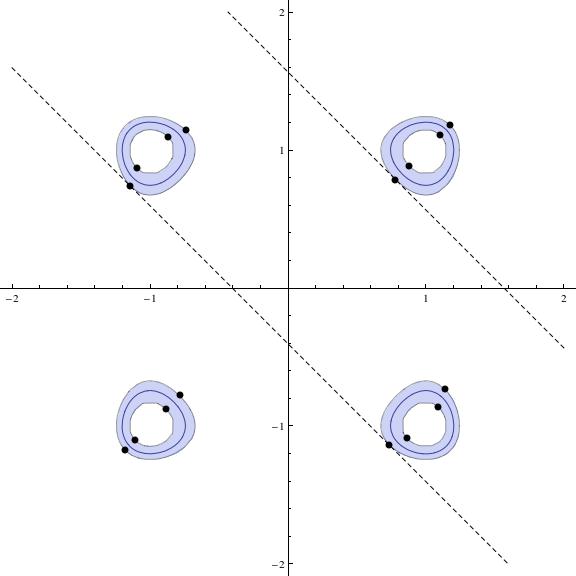
Figure 1. The real variety $\mathrm{Zer}\left(P,\mathbf{R}^{2}\right)$, and the set defined by $\operatorname{Def}(P,\zeta,6)\leq 0$, in Example 2.

Example 2.

In this example, the number of blocks $\omega=1$, and $k=k_{1}=2$. Consider the polynomial

$$P = (X_{1}^{2}-1)^{2}+(X_{2}^{2}-1)^{2}-\varepsilon,$$

for some small $\varepsilon\char 62\relax 0$. The sets $\mathrm{Zer}\left(P,\mathbf{R}^{2}\right)$, and $S=\left\{x\in\mathbf{R}\langle\zeta\rangle^{2}\mid\bar{P}\leq 0\right\}$, where $\bar{P}=\operatorname{Def}(P,\zeta,6)$ is shown in the Figure 1.

The polynomial $e_{1}(X_{1},X_{2})=X_{1}+X_{2}$ has $16$ critical points, corresponding to $12$ critical values, $v_{1}\char 60\relax\cdots\char 60\relax v_{12}$, on $\mathrm{Zer}\left(\bar{P},\mathbf{R}\langle\zeta\rangle^{2}\right)$ of which $v_{5}$ and $v_{9}$ are indicated in Figure 1 using dotted lines. The corresponding indices of the critical points, the number of critical points for each critical value, the sign of the polynomial $\dfrac{\partial\bar{P}}{\partial X_{1}}+\dfrac{\partial\bar{P}}{\partial X_{2}}$ at these critical points, and the partition $\pi\in\Pi_{2}$ such that the corresponding critical points belong to $L_{\pi}$ are shown in Table 1. The critical points corresponding to the shaded rows are the the critical points where $\left(\dfrac{\partial\bar{P}}{\partial X_{1}}+\dfrac{\partial\bar{P}}{\partial X_{2}}\right)\char 60\relax 0$, and these are the critical points whose orbits are represented in the sets $G_{c}^{-}$ in Lemma 6 above.

Critical values	Index	$\operatorname{SIGN}\left(\dfrac{\partial\bar{P}}{\partial X_{1}}+\dfrac{\partial\bar{P}}{\partial X_{2}}\right)$	$\pi$	$L^{-}(p)$	$L_{\mathrm{fixed}}$	$L^{-}(p)\subset L_{\mathrm{fixed}}$
$v_{1}$	0	$-1$	$(2)$	$0$	$0$	yes
$v_{2}$	0	$1$	$(2)$	0	$0$	yes
$v_{3}$	1	$-1$	$(2)$	$L$	$0$	no
$v_{4}$	1	$1$	$(2)$	$L$	$0$	no
$v_{5}$	$0$	$-1$	$(1,1)$	$0$	$L$	yes
$v_{6}$	0	1	$(1,1)$	$0$	$L$	yes
$v_{7}$	$1$	$-1$	$(1,1)$	$L$	$L$	yes
$v_{8}$	$1$	$1$	$(1,1)$	$L$	$L$	yes
$v_{9}$	$0$	$-1$	$(2)$	$0$	$0$	yes
$v_{10}$	0	$1$	$(2)$	$0$	$0$	yes
$v_{11}$	$1$	$-1$	$(2)$	$L$	$0$	no
$v_{12}$	$1$	1	$(2)$	$L$	$0$	no

Table 1. Table of critical values in Example 2.

Proof of Proposition 6.

The proposition follows directly from Lemmas 5 and 6, after noting that at most half the critical values of $F$ satisfy (28) of Lemma 6. ∎

5. Proofs of the main theorems

We are now in a position to prove the main theorems.

5.1. Proof of Theorem 6

Proof of Theorem 6.

By Remark 1, we can assume without loss of generality that $P$ is symmetric in each block of variables $X^{(1)},\ldots,X^{(\omega)}$. We first assume that $\mathrm{Zer}\left(P,\mathbf{R}^{k}\right)$ is bounded. Let $d^{\prime}$ be the least even number such that $d^{\prime}\char 62\relax d=\deg(P)$ and such that $d^{\prime}-1$ is prime. By Bertrand’s postulate we have that $d^{\prime}\leq 2d$. Now, if $p$ divides $k$, replace $P$ by the polynomial

$$P+X_{k+1}^{2},$$

and let $\omega^{\prime}=\omega+1$, $k^{\prime}=k+1$, and $\mathbf{k}^{\prime}=(\mathbf{k},1)$. Otherwise, let $\omega^{\prime}=\omega+1$, $k^{\prime}=k$, and $\mathbf{k}^{\prime}=(\mathbf{k},0)$. In either case, we have that $\gcd(p,k^{\prime})=1$, and $k^{\prime}\leq k+1$.

Using Proposition 3,

$$b(\phi_{\mathbf{k}}(V),\mathbb{F}) = b(\phi_{\mathbf{k}^{\prime}}(S),\mathbb{F})$$

where $S$ is the semi-algebraic set defined by $\operatorname{Def}(P,\zeta,d^{\prime})\leq 0$. It now follows from Propositions 4, 5, 6 , and Bezout’s theorem that

$$b(\phi_{\mathbf{k}^{\prime}}(S),\mathbb{F}) \leq \frac{1}{2}\sum_{\begin{subarray}{c}\bm{\pi}=(\pi^{(1)},\ldots,\pi^{(\omega^{\prime})})\in\bm{\Pi}_{\mathbf{k}^{\prime}},\\ \mathrm{length}(\pi^{(i)})\leq d^{\prime},\\ 1\leq i\leq\omega^{\prime}\end{subarray}}d^{\prime}(d^{\prime}-1)^{\mathrm{length}(\bm{\pi})-1}.$$

After noting that using Bertrand’s postulate $d^{\prime}\leq 2d$, and using the fact that $k^{\prime}\leq k+1$, we obtain that in the bounded case,

$$b(\phi_{\mathbf{k}}(V),\mathbb{F}) \leq \sum_{\begin{subarray}{c}\bm{\ell}^{\prime}=(\ell_{1},\ldots,\ell_{\omega^{\prime}}),\\ 1\leq\ell_{i}\leq\min(k_{i},2d)\end{subarray}}p(\mathbf{k}^{\prime},\bm{\ell}^{\prime})d(2d-1)^{\char 124\relax\bm{\ell}^{\prime}\char 124\relax-1}$$

Eqn. (15) follows from Eqn. (27) in Proposition 6.

To take of the possibly unbounded case we introduce a new variable $Z$, and let

$$P_{1} = P+\left(Z^{2}+\sum_{i=1}^{k}X_{i}^{2}+\sum_{j=1}^{m}Y_{j}^{2}-\Omega^{2}\right)^{2},$$

$$P_{2} = P+\left(\sum_{i=1}^{k}X_{i}^{2}+\sum_{j=1}^{m}Y_{j}^{2}-\Omega^{2}\right)^{2}.$$

Notice that, $V_{1}=\left(\mathrm{Zer}\left(P_{1},\mathbf{R}\left\langle\tfrac{1}{\Omega}\right\rangle^{k+1}\right)\right)$ is semi-algebraically homeomorphic to two homeomorphic copies of $V_{2}=\left(\mathrm{Zer}\left(P_{2},\mathbf{R}\left\langle\tfrac{1}{\Omega}\right\rangle^{k}\right)\right)$ glued along $V$.

Using the fact that the map $\phi_{\mathbf{k}}$ is proper, it now follows from inequality (20) that

$$b(\phi_{\mathbf{k}}(V),\mathbb{F}) \leq \frac{1}{2}(b(\phi_{(\mathbf{k},1)}(V_{1}),\mathbb{F})+b(\phi_{\mathbf{k}}(V_{2}),\mathbb{F})).$$

Noticing that both $\mathrm{Zer}\left(P_{1},\mathbf{R}\left\langle\tfrac{1}{\Omega}\right\rangle^{k+1}\right)$ and $\mathrm{Zer}\left(P_{2},\mathbf{R}\left\langle\tfrac{1}{\Omega}\right\rangle^{k}\right)$ are bounded, we can use the result from the bounded case and obtain in general that for $d\geq 4$,

$$b(\phi_{\mathbf{k}}(V),\mathbb{F}) \leq \sum_{\begin{subarray}{c}\bm{\ell}^{\prime}=(\ell_{1},\ldots,\ell_{\omega^{\prime}}),\\ 1\leq\ell_{i}\leq\min(k_{i},2d)\end{subarray}}(p(\mathbf{k}^{\prime},\bm{\ell}^{\prime}))d(2d-1)^{\char 124\relax\bm{\ell}^{\prime}\char 124\relax}$$

$$\leq \sum_{\begin{subarray}{c}\bm{\ell}=(\ell_{1},\ldots,\ell_{\omega}),\\ 1\leq\ell_{i}\leq\min(k_{i},2d)\end{subarray}}(p(\mathbf{k},\bm{\ell}))d(2d-1)^{\char 124\relax\bm{\ell}\char 124\relax+1},$$

where the last inequality follows from the fact that $\omega^{\prime}=\omega+1$, and $k_{\omega^{\prime}}=1$. ∎

5.2. Proof of Theorem 7

Definition 2.

For any finite family $\mathcal{P}\subset\mathbf{R}[X_{1},\ldots,X_{k}]$ and $\ell\geq 0$, we say that $\mathcal{P}$ is in $\ell$-general position with respect to a semi-algebraic set $V\subset\mathbf{R}^{k}$ if for any subset $\mathcal{P}^{\prime}\subset\mathcal{P}$, with $\mathrm{card}(\mathcal{P}^{\prime})\char 62\relax\ell$, $\mathrm{Zer}(\mathcal{P}^{\prime},V)=\emptyset$.

Let $\mathbf{k}=(k_{1},\ldots,k_{\omega})$ with $k=\sum_{i=1}^{\omega}k_{i}$, and

$$\mathcal{P}=\{P_{1},\ldots,P_{s}\}\subset\mathbf{R}[\mathbf{X}^{(1)},\ldots,\mathbf{X}^{(\omega)}]^{\mathfrak{S}_{\mathbf{k}}}$$

be a fixed finite set of polynomials where $\mathbf{X}^{(i)}$ is a block of $k_{i}$ variables. Let $\deg(P_{i})\leq d$ for $1\leq i\leq s$. Let $\overline{\varepsilon}=\left(\varepsilon_{1},\ldots,\varepsilon_{s}\right)$ be a tuple of new variables, and let $\mathcal{P}_{\overline{\varepsilon}}=\bigcup_{1\leq i\leq s}\left\{P_{i}\pm\varepsilon_{i}\right\}$. We have the following two lemmas.

Lemma 7.

Let

$$D^{\prime}(\mathbf{k},d) = \sum_{i=1}^{\omega}\min(k_{i},d).$$

The set of polynomials $\mathcal{P}_{\overline{\varepsilon}}\subset\mathbf{R}^{\prime}[\mathbf{X}^{(1)},\ldots,\mathbf{X}^{(\omega)}]$ is in $D^{\prime}$-general position for any semi-algebraic subset $Z\subset\mathbf{R}^{k}$ stable under the action of $\mathfrak{S}_{\mathbf{k}}$, where $\mathbf{R}^{\prime}=\mathbf{R}\langle\overline{\varepsilon}\rangle$.

Proof.

Using Lemma 1 for each $i,1\leq i\leq s$, there exists $\widetilde{P}_{i}\in\mathbf{R}[\mathbf{Z}^{(1)},\ldots,\mathbf{Z}^{(\omega)}]$, where each $Z^{(i)}$ is a block of $\ell_{i}=\min(k_{i},d)$ variables such that

$$P_{i} = \widetilde{P}_{i}((p_{1}^{(k_{1})}(\mathbf{X}^{(1)}),\ldots,p_{\ell_{1}}^{(k_{1})}(\mathbf{X}^{(1)})),\ldots,(p_{1}^{(k_{\omega})}(\mathbf{X}^{(\omega)}),\ldots,p_{\ell_{\omega}}^{(k_{\omega})}(\mathbf{X}^{(\omega)}))).$$

Clearly,

$$\halign{\hbox to\displaywidth{$\hfil\displaystyle#\hfil$}\cr 0.0pt{\hfil$\displaystyle P_{i}\pm\varepsilon_{i}=\cr 0.0pt{\hfil$\displaystyle\widetilde{P}_{i}((p_{1}^{(k_{1})}(\mathbf{X}^{(1)}),\ldots,p_{\ell_{1}}^{(k_{1})}(\mathbf{X}^{(1)})),\ldots,(p_{1}^{(k_{\omega})}(\mathbf{X}^{(\omega)}),\ldots,p_{\ell_{\omega}}^{(k_{\omega})}(\mathbf{X}^{(\omega)})))\pm\varepsilon_{i}.\crcr}}}$$

Since no sub-collection of the polynomials $\bigcup\limits_{1\leq i\leq s}\left\{\widetilde{P}_{i}\pm\varepsilon_{i}\right\}$ of cardinality at least

$$1+\sum\limits_{i=1}^{\omega}\min(k_{i},d)=D^{\prime}+1$$

can have a common zero in $\mathbf{R}^{\prime D^{\prime}}$, the lemma follows.∎

Let $\Phi$ be a $\mathcal{P}$-closed formula, and let $S=\mathrm{Reali}(\Phi,V)$ be bounded over $\mathbf{R}$. Let $\Phi_{\overline{\varepsilon}}$ be the $\mathcal{P}_{\overline{\varepsilon}}$-closed formula obtained from $\Phi$ be replacing for each $i,1\leq i\leq s$,

1. each occurrence of $P_{i}\leq 0$ by $P_{i}-\varepsilon_{i}\leq 0$, and

2. each occurrence of $P_{i}\geq 0$ by $P_{i}+\varepsilon_{i}\geq 0$.

Let $\mathbf{R}^{\prime}=\mathbf{R}\left\langle\varepsilon_{1},\ldots,\varepsilon_{s}\right\rangle$, and  $S_{\overline{\varepsilon}}=\mathrm{Reali}\left(\Phi_{\overline{\varepsilon}},\mathbf{R}^{\prime k}\right)$.

Lemma 8.

For any $r\char 62\relax 0$, $r\in\mathbf{R}$, the semi-algebraic set $\operatorname{Ext}(S\cap\overline{B_{k}(0,r)},\mathbf{R}^{\prime})$ is contained in $S_{\overline{\varepsilon}}\cap\overline{B_{k}(0,r)}$, and the inclusion $\operatorname{Ext}(S\cap\overline{B_{k}(0,r)},\mathbf{R}^{\prime})\hookrightarrow S_{\overline{\varepsilon}}\cap\overline{B_{k}(0,r)}$ is a semi-algebraic homotopy equivalence.

Moreover, $\operatorname{Ext}(S\cap\overline{B_{k}(0,r)},\mathbf{R}^{\prime})/\mathfrak{S}_{\mathbf{k}}\subset(S_{\overline{\varepsilon}}\cap\overline{B_{k}(0,r)})/\mathfrak{S}_{\mathbf{k}}$, and the inclusion map $\operatorname{Ext}(S\cap\overline{B_{k}(0,r)},\mathbf{R}^{\prime})/\mathfrak{S}_{\mathbf{k}}\hookrightarrow\left(S_{\overline{\varepsilon}}\cap\overline{B_{k}(0,r)}\right)/\mathfrak{S}_{\mathbf{k}}$ is a semi-algebraic homotopy equivalence.

Proof.

The proof is similar to the one of Lemma 16.17 in [6]. ∎

Remark 9.

In view of Lemmas 7 and 8 we can assume (at the cost of doubling the number of polynomials) after possibly replacing $\mathcal{P}$ by $\mathcal{P}_{\overline{\varepsilon}}$, and $\mathbf{R}$ by $\mathbf{R}^{\prime}$, that the family $\mathcal{P}$ is in $D^{\prime}(\mathbf{k},d)$-general position.

Now, let $\delta_{1},\cdots,\delta_{s}$ be new infinitesimals, and let $\mathbf{R}^{\prime\prime}=\mathbf{R}^{\prime}\langle\delta_{1},\ldots,\delta_{s}\rangle$.

Notation 20.

We define $\mathcal{P}_{\char 62\relax i}=\{P_{i+1},\ldots,P_{s}\}$ and

$$\Sigma_{i} = \{P_{i}=0,P_{i}=\delta_{i},P_{i}=-\delta_{i},P_{i}\geq 2\delta_{i},P_{i}\leq-2\delta_{i}\},$$

$$\Sigma_{\leq i} = \{\Psi\mid\Psi=\bigwedge_{j=1,\ldots,i}\Psi_{i},\Psi_{i}\in\Sigma_{i}\}.$$

Note that for each $\Psi\in\Sigma_{i}$, $\mathrm{Reali}(\Psi,\mathbf{R}^{\prime}\langle\delta_{1},\ldots,\delta_{i}{k})$ is symmetric with respect to the action of $\mathfrak{S}_{\mathbf{k}}$ and for if $\Psi\neq\Psi^{\prime}$, $\Psi,\Psi^{\prime}\in\Sigma_{\leq i}$,

(31) $$\mathrm{Reali}(\Psi,\mathbf{R}^{\prime}\langle\delta_{1},\ldots,\delta_{i}\rangle^{k})\cap\mathrm{Reali}(\Psi^{\prime},\mathbf{R}^{\prime}\langle\delta_{1},\ldots,\delta_{i}\rangle^{k}) = \emptyset.$$

If $\Phi$ is a $\mathcal{P}$-closed formula, we denote

$$\mathrm{Reali}_{i}(\Phi) = \mathrm{Reali}(\Phi,\mathbf{R}^{\prime}\langle\delta_{1},\ldots,\delta_{i}\rangle^{k}),$$

and

$$\mathrm{Reali}_{i}(\Phi\wedge\Psi) = \mathrm{Reali}(\Psi,\mathbf{R}^{\prime}\langle\delta_{1},\ldots,\delta_{i}\rangle^{k})\cap\mathrm{Reali}_{i}(\Phi).$$

Finally, we denote for each $\mathcal{P}$-closed formula $\Phi$

$$b(\Phi/\mathfrak{S}_{\mathbf{k}},\mathbb{F}) = b(\mathrm{Reali}(\Phi,\mathbf{R}^{\prime\prime k})/\mathfrak{S}_{\mathbf{k}},\mathbb{F}).$$

The proof of the following proposition is very similar to Proposition 7.39 in [6] where it is proved in the non-symmetric case.

Proposition 8.

For every $\mathcal{P}$-closed formula $\Phi$, such that $\mathrm{Reali}(\Phi,\mathbf{R}^{k})$ is bounded,

$$b(\Phi/\mathfrak{S}_{\mathbf{k}},\mathbb{F}) \leq \sum_{\begin{subarray}{c}\Psi\in\Sigma_{\leq s}\\ \mathrm{Reali}_{s}(\Psi,\mathbf{R}^{\prime\prime k})\subset\mathrm{Reali}_{s}(\Phi,\mathbf{R}^{\prime\prime k})\end{subarray}}b(\Psi/\mathfrak{S}_{\mathbf{k}},\mathbb{F}).$$

Proof.

First observe that the orbit space of a disjoint union of symmetric sets is a disjoint union of the corresponding orbit spaces. The symmetric semi-algebraic sets $\mathrm{Reali}(\Psi,\mathbf{R}^{\prime\prime k}),\Psi\in\Sigma_{\leq s}$ are disjoint by (31). The proof is now the same as the proof of Proposition 7.39 in [6]. ∎

Let

$$D^{\prime}=D^{\prime}(\mathbf{k},d) = \sum^{\omega}_{i=1}\min(k_{i},d),$$

$$D^{\prime\prime}=D^{\prime\prime}(\mathbf{k},d) = \sum^{\omega}_{i=1}\min(k_{i},4d).$$

Proposition 9.

For $0\leq i\char 60\relax D^{\prime}+D^{\prime\prime}$,

$$\sum_{\Psi\in\Sigma_{\leq s}}b_{i}(\Psi/\mathfrak{S}_{\mathbf{k}},\mathbb{F})\leq\sum_{j=0}^{D^{\prime}+D^{\prime\prime}-i}\binom{s}{j}6^{j}F(\mathbf{k},2d).$$

For $i\geq D^{\prime}+D^{\prime\prime}$,

$$\sum_{\Psi\in\Sigma_{\leq s}}b_{i}(\Psi/\mathfrak{S}_{\mathbf{k}},\mathbb{F})=0.$$

We first prove the following lemmas. Let $Q_{i}=P_{i}^{2}(P_{i}^{2}-\delta_{i}^{2})^{2}(P_{i}^{2}-4\delta_{i}^{2})$.

For $j\geq 1$ let,

$$V_{j} = \mathrm{Reali}(\bigvee_{1\leq i\leq j}Q_{i}=0,\mathbf{R}^{\prime}\langle\delta_{1},\ldots,\delta_{j}\rangle^{k}),$$

$$W_{j} = \mathrm{Reali}(\bigvee_{1\leq i\leq j}Q_{i}\geq 0,\mathbf{R}^{\prime}\langle\delta_{1},\ldots,\delta_{j}\rangle^{k}).$$

Lemma 9.

Let $I\subset[1,s]$, $\sigma=(\sigma_{1},\ldots,\sigma_{s})\in\{0,\pm 1,\pm 2\}^{s}$ and let

$$\mathcal{P}_{I,\sigma}=\bigcup_{i\in I}\{P_{i}+\sigma_{i}\delta_{i}\}.$$

Then, $\mathrm{Zer}(\mathcal{P}_{I,\sigma},\mathbf{R}^{\prime\prime k})=\emptyset$, whenever $\mathrm{card}(I)\char 62\relax D^{\prime}$.

Proof.

This follows from the fact that $\mathcal{P}$ is in $D^{\prime}$-general position by Remark 9. ∎

Lemma 10.

For each $i,0\leq i\char 60\relax D^{\prime}+D^{\prime\prime}$,

$$b_{i}(V_{j}/\mathfrak{S}_{\mathbf{k}},\mathbb{F})\leq(6^{j}-1)F(\mathbf{k},2d).$$

For $i\geq D^{\prime}+D^{\prime\prime}$,

$$b_{i}(V_{j}/\mathfrak{S}_{\mathbf{k}},\mathbb{F}) = 0.$$

Proof.

Clearly, $V_{j}$ is the disjoint union of the real varieties

$$\halign{\hbox to\displaywidth{$\hfil\displaystyle#\hfil$}\cr 0.0pt{\hfil$\displaystyle\mathrm{Zer}(P_{i},\mathbf{R}^{\prime}\langle\delta_{1},\ldots,\delta_{j}\rangle^{k}),\cr 0.0pt{\hfil$\displaystyle\mathrm{Zer}(P_{i}\pm\delta_{i},\mathbf{R}^{\prime}\langle\delta_{1},\ldots,\delta_{j}\rangle^{k}),\cr 0.0pt{\hfil$\displaystyle\mathrm{Zer}(P_{i}\pm 2\delta_{i},\mathbf{R}^{\prime}\langle\delta_{1},\ldots,\delta_{j}\rangle^{k}),\crcr}}}}$$

for $1\leq i\leq j$, and hence the quotient $V_{j}/\mathfrak{S}_{\mathbf{k}}$ is the disjoint union of the quotients

$$\mathrm{Zer}(P_{i},\mathbf{R}^{\prime}\langle\delta_{1},\ldots,\delta_{j}\rangle^{k})/\mathfrak{S}_{\mathbf{k}},$$

(32) $$\mathrm{Zer}(P_{i}\pm\delta_{i},\mathbf{R}^{\prime}\langle\delta_{1},\ldots,\delta_{j}\rangle^{k})/\mathfrak{S}_{\mathbf{k}},$$

$$\mathrm{Zer}(P_{i}\pm 2\delta_{i},\mathbf{R}^{\prime}\langle\delta_{1},\ldots,\delta_{j}\rangle^{k})/\mathfrak{S}_{\mathbf{k}}.$$

It follows from Part (A) of Proposition 2 that $b_{i}(V_{j}/\mathfrak{S}_{\mathbf{k}},\mathbb{F})$ is bounded by the sum for $1\leq\ell\leq i+1$, of $(i-\ell+1)$-th Betti numbers of all possible $\ell$-ary intersections amongst quotients of the varieties listed above. It is clear that the total number of such non-empty $\ell$-ary intersections is at most $\binom{j}{\ell}5^{\ell}$. It now follows from Theorem 6 applied to the non-negative symmetric polynomials $P_{i}^{2},(P_{i}\pm\delta_{i})^{2},(P_{i}\pm 2\delta_{i})^{2}$, and noting that the degrees of these polynomials are bounded by $2d$, that

$$b_{i}(V_{j}/\mathfrak{S}_{\mathbf{k}},\mathbb{F}) \leq \sum_{p=1}^{\min(j,D^{\prime})}\binom{j}{p}5^{p}F(\mathbf{k},2d).$$

To prove the vanishing of the higher Betti numbers, first observe that $(i-\ell+1)$-th Betti numbers of all possible $\ell$-ary intersections amongst the sets listed in (32) vanish for $i-\ell+1\char 62\relax D^{\prime\prime}$ using Theorem 6.

Also, notice that by Lemma 9 the $\ell$-ary intersections amongst the sets in (32) are empty for $\ell\char 62\relax D^{\prime}$. Together, these observations imply that

$$b_{i}(V_{j}/\mathfrak{S}_{\mathbf{k}},\mathbb{F}) = 0.$$

for all $i\geq D^{\prime}+D^{\prime\prime}$. To see this observe that if $i\geq D^{\prime}+D^{\prime\prime}$, and $\ell\leq D^{\prime}$, then $i-\ell+1\geq D^{\prime\prime}+1$. ∎

Lemma 11.

For $0\leq i\char 60\relax D^{\prime}+D^{\prime\prime}$,

$$b_{i}(W_{j}/\mathfrak{S}_{\mathbf{k}},\mathbb{F})\leq\sum_{p=1}^{\min(j,D^{\prime})}\binom{j}{p}5^{p}(F(\mathbf{k},2d))+b_{i}(\mathbf{R}^{\prime}\langle\delta_{1},\ldots,\delta_{j}\rangle^{k}/\mathfrak{S}_{k},\mathbb{F}).$$

For $i\geq D^{\prime}+D^{\prime\prime}$, $b_{i}(W_{j}/\mathfrak{S}_{\mathbf{k}},\mathbb{F})=0$.

Proof.

Let

$$W^{\prime}_{j}=\mathrm{Reali}(\bigwedge_{1\leq i\leq j}Q_{i}\leq 0\vee\bigvee_{1\leq i\leq j}Q_{i}=0,\mathbf{R}^{\prime}\langle\delta_{1},\ldots,\delta_{j}\rangle)^{k}).$$

Now, from the fact that

$$W_{j}\cup W^{\prime}_{j}=\mathbf{R}^{\prime}\langle\delta_{1},\ldots,\delta_{j}\rangle^{k},W_{j}\cap W^{\prime}=V_{j},$$

it follows immediately that

$$(W_{j}\cup W^{\prime}_{j})/\mathfrak{S}_{\mathbf{\mathbf{k}}}=(W_{j}/\mathfrak{S}_{\mathbf{k}})\cup(W^{\prime}_{j}/\mathfrak{S}_{\mathbf{k}})=\mathbf{R}^{\prime}\langle\delta_{1},\ldots,\delta_{j}\rangle^{k}/\mathfrak{S}_{\mathbf{k}},$$

and

$$(W_{j}/\mathfrak{S}_{\mathbf{k}})\cap(W^{\prime}_{j}/\mathfrak{S}_{\mathbf{k}})=(W_{j}\cap W^{\prime}_{j})/\mathfrak{S}_{\mathbf{k}}=V_{j}/\mathfrak{S}_{\mathbf{k}}.$$

Using inequality (20) we get that

$$b_{i}(W_{j}/\mathfrak{S}_{\mathbf{k}},\mathbb{F}) \leq b_{i}((W_{j}\cap W^{\prime}_{j})/\mathfrak{S}_{\mathbf{k}},\mathbb{F})+b_{i}((W_{j}\cup W^{\prime}_{j})/\mathfrak{S}_{\mathbf{k}},\mathbb{F})$$

$$= b_{i}(V_{j}/\mathfrak{S}_{\mathbf{k}},\mathbb{F})+b_{i}(\mathbf{R}^{\prime}\langle\delta_{1},\ldots,\delta_{j}\rangle^{k}/\mathfrak{S}_{\mathbf{k}},\mathbb{F})$$

We conclude using Lemma 10. ∎

Proof of Proposition 9.

Using Part (B) of Proposition 2 we get that

$$\sum_{\Psi\in\Sigma_{\leq s}}b_{i}(\Psi/\mathfrak{S}_{\mathbf{k}},\mathbb{F}) \leq \sum_{j=1}^{k-i}\sum_{\begin{subarray}{c}J\subset\{1,\ldots,s\}\\ \mathrm{card}(J)=j\end{subarray}}b_{i+j-1}(S^{J}/\mathfrak{S}_{\mathbf{k}},\mathbb{F})+\binom{s}{k-i}b_{k}(S^{\emptyset}/\mathfrak{S}_{\mathbf{k}},\mathbb{F}).$$

It follows from Lemma 11 that,

$$b_{i+j-1}(S^{J}/\mathfrak{S}_{\mathbf{k}},\mathbb{F}) = 0,$$

when $i+j-1\geq D^{\prime}+D^{\prime\prime}$, and otherwise,

$$b_{i+j-1}(S^{J}/\mathfrak{S}_{\mathbf{k}},\mathbb{F}) \leq \sum_{\ell=1}^{\min(j,D^{\prime})}\binom{j}{\ell}5^{\ell}F(\mathbf{k},2d)+b_{k}(\mathbf{R}^{k}/\mathfrak{S}_{\mathbf{k}},\mathbb{F}).$$

Hence,

$$\sum_{\Psi\in\Sigma_{\leq s}}b_{i}(\Psi/\mathfrak{S}_{\mathbf{k}},\mathbb{F}) \leq \sum_{j=1}^{D^{\prime}+D^{\prime\prime}-i}\sum_{\begin{subarray}{c}J\subset\{1,\ldots,s\}\\ \mathrm{card}(J)=j\end{subarray}}b_{i+j-1}(S^{J}/\mathfrak{S}_{\mathbf{k}})+$$

$$\binom{s}{k-i}b_{k}(S^{\emptyset}/\mathfrak{S}_{\mathbf{k}})$$

$$\leq \sum_{j=1}^{D^{\prime}+D^{\prime\prime}-i}\binom{s}{j}\left(\sum_{p=1}^{\min(j,D^{\prime})}\binom{j}{p}5^{p}F(\mathbf{k},2d)\right)$$

$$\leq \sum_{j=1}^{D^{\prime}+D^{\prime\prime}-i}\binom{s}{j}6^{j}F(\mathbf{k},2d).$$

Finally, it is clear that

$$\sum_{\Psi\in\Sigma_{\leq s}}b_{i}(\Psi/\mathfrak{S}_{\mathbf{k}},\mathbb{F}) = 0,$$

for $i\geq D+D^{\prime}$.

∎

Proof of Theorem 7.

We add an extra polynomial, $\delta(X_{1}^{2}+\cdots+X_{k}^{2})-1$ to the set $\mathcal{P}$, replace the field $\mathbf{R}$, by $\mathbf{R}\langle\delta\rangle$, and replace the given formula $\mathcal{P}$-closed formula $\Phi$ by the formula $\Phi\wedge(\delta(X_{1}^{2}+\cdots+X_{k}^{2})-1\leq 0)$. Notice that the new set $\mathrm{Reali}(\Phi)$ is bounded in $\mathbf{R}\langle\delta\rangle^{k}$ and has isomorphic homology groups as $S$.

We first consider the case in which for each $i,1\leq i\leq\omega$, $4d\leq k_{i}$. In this case,

$$D(\mathbf{k},d) = D^{\prime}(\mathbf{k},d)+D^{\prime\prime}(\mathbf{k},d),$$

and Theorem 7 follows from Propositions 8 and 9, recalling that the number of polynomials was doubled in ordered to put the family $\mathcal{P}$ in $D^{\prime}$-general position. In the general case, suppose without loss of generality that $k_{i}\leq 4d$, for $1\leq i\leq\omega^{\prime}\leq\omega$, and $k_{i}\char 62\relax 4d$ for $i\char 62\relax\omega^{\prime}$. Let, $\mathbf{k}^{\prime}=(k_{1},\ldots,k_{\omega^{\prime}})$, $k^{\prime}=\sum_{i=1}^{\omega^{\prime}}k_{i}$, and $\bar{\pi}:\mathbf{R}^{k}/\mathfrak{S}_{\mathbf{k}}\rightarrow\mathbf{R}^{k^{\prime}}/\mathfrak{S}_{\mathbf{k}^{\prime}}$ the map induced by the projection map, $\pi:\mathbf{R}^{k}\rightarrow\mathbf{R}^{k^{\prime}}$, to the first $k^{\prime}$ coordinates.

Then, for each $\bar{\mathbf{y}}\in\bar{\pi}(S/\mathfrak{S}_{\mathbf{k}})$, we have by applying the special case of Theorem 7 already proved above that,

$$b_{i}((S\cap\pi^{-1}(\bar{\mathbf{y}}))/\mathfrak{S}_{\mathbf{k}}),\mathbb{F}) = 0,$$

for $i\geq\sum_{i=\omega^{\prime}+1}^{\omega}\left(\min(k_{i},4d)+\min(k_{i},d)\right)=5(\omega-\omega^{\prime})d$.

In other words, the the fibers of the map $\bar{\pi}:\mathbf{R}^{k}/\mathfrak{S}_{\mathbf{k}}\rightarrow\mathbf{R}^{k^{\prime}}/\mathfrak{S}_{\mathbf{k}^{\prime}}$ restricted to $S/\mathfrak{S}_{k}$ have vanishing homology above (and including) dimension $5(\omega-\omega^{\prime})d$, and clearly the image of the map has dimension $\leq k^{\prime}$.

It now follows from Leray spectral sequence of the map $\bar{\pi}:\mathbf{R}^{k}/\mathfrak{S}_{\mathbf{k}}\rightarrow\mathbf{R}^{k^{\prime}}/\mathfrak{S}_{\mathbf{k}^{\prime}}$ restricted to $S/\mathfrak{S}_{k}$ (see for example [17, Théorème 5.2.4]), that

$$b_{i}(S/\mathfrak{S}_{\mathbf{k}},\mathbb{F}) = 0,$$

for $i\geq k^{\prime}+5(\omega-\omega^{\prime})d=D(\mathbf{k},d)$.

A similar argument proves that in Proposition 9 we can replace $D^{\prime}+D^{\prime\prime}$ by $D$ as well.

This proves the theorem in general.∎

5.3. Proof of Theorem 8

In [14], Gabrielov and Vorobjov introduced a construction for replacing an arbitrary $\mathcal{P}$-semi-algebraic set $S$ by a certain $\mathcal{P}^{\prime}_{p}$-closed semi-algebraic set $S_{p}^{\prime}$ (for any given $p\geq 0$), such that $S$ and $S_{p}^{\prime}$ are $p$-equivalent. The family $\mathcal{P}^{\prime}_{p}$ in their construction is given by

$$\mathcal{P}_{p}^{\prime} = \bigcup_{P\in\mathcal{P}}\bigcup_{0\leq i\leq p}\left\{P\pm\varepsilon_{i},P\pm\delta_{i}\right\},$$

where the $\varepsilon_{i},\delta_{i}$ are infinitesimals.

Note that $\mathcal{P}\subset\mathbf{R}[\mathbf{X}^{(1)},\ldots,\mathbf{X}^{(\omega)}]^{\mathfrak{S}_{\mathbf{k}}}$ implies that $\mathcal{P}^{\prime}_{p}\subset\mathbf{R}[\mathbf{X}^{(1)},\ldots,\mathbf{X}^{(\omega)}]^{\mathfrak{S}_{\mathbf{k}}}$ as well, and if the degrees of the polynomials in $\mathcal{P}$ are bounded by $d$, the same bound applies to polynomials in $\mathcal{P}^{\prime}_{p}$ as well. Furthermore, $\mathrm{card}(\mathcal{P}^{\prime}_{p})=4(p+1)\mathrm{card}(\mathcal{P})$. It is an immediate consequence of the above result that $S/\mathfrak{S}_{\mathbf{k}}$ is $p$-equivalent to $S^{\prime}/\mathfrak{S}_{\mathbf{k}}$ as well.

Proof of Theorem 8.

Using the above construction, replace $S$ by $S_{p}^{\prime}$, with $p=k$. Then, apply Theorem 7.∎

5.4. Proof of Theorem 10

We now prove Theorem 10 closely following the proof of Theorem 9 in [15]. We first need a few preliminary definitions and notation.

For the rest of this section we fix $X$ to be a compact semi-algebraic subset of $\mathbf{R}$.

Notation 21 (Standard simplex).

We will denote by $\Delta_{p}$, the standard $p$-dimensional simplex, namely

$$\Delta_{p} = \{(s_{0},\ldots,s_{p})\char 124\relax s_{0},\ldots,s_{p}\geq 0,s_{0}+\cdots+s_{p}=1\}.$$

Notation 22 (Symmetric product).

We denote for each $p\geq 0$, $\mathrm{Sym}^{(p)}(X)$ the $(p+1)$-fold symmetric product of $X$ i.e.

$$\mathrm{Sym}^{(p)}(X) = \underbrace{X\times\cdots\times X}_{p+1}/\mathfrak{S}_{p+1}.$$

Let $\mathcal{W}^{(p)}=\{\mathbf{x}=(x_{0},\ldots,x_{p})\in\mathbf{R}^{p+1}\mid x_{0}\leq x_{1}\leq\cdots\leq x_{p}\}$ Then, $\mathrm{Sym}^{(p)}(X)$ is homeomorphic to $X^{p+1}\cap\mathcal{W}^{(p)}$, and we will identify $\mathrm{Sym}^{(p)}(X)$ with the set $X^{p+1}\cap\mathcal{W}^{(p)}$.

Definition 3 (Symmetric join).

We next define $J^{(p)}_{\mathrm{symm}}(X)$ as follows.

$$J^{(p)}_{\mathrm{symm}}(X) = \mathrm{Sym}^{(p)}(X)\times\Delta_{p}/\sim,$$

where the equivalence relation $\sim$ is given by (after identifying $\mathrm{Sym}^{(p)}(X)$ with $X^{p+1}\cap\mathcal{W}^{(p)}$ cf. Notation 22)

$$((x_{0},\ldots,x_{p}),(s_{0},\ldots,s_{p}))\sim((x_{0}^{\prime},\ldots,x_{p}^{\prime}),(s_{0}^{\prime},\ldots,s_{p}^{\prime}))$$

if and only if $(s_{0},\ldots,s_{p})=(s_{0}^{\prime},\ldots,s_{p}^{\prime})$, and $x_{i}=x_{i}^{\prime}$ for all $i$ such that $s_{i}=s_{i}^{\prime}\neq 0$.

For each $p\char 62\relax 0,0\leq i\leq p$, there is an injection

$$\phi^{(p,i)}:J^{(p-1)}_{\mathrm{symm}}(X)\rightarrow J^{(p)}_{\mathrm{symm}}(X)$$

defined by

$$\halign{\hbox to\displaywidth{$\hfil\displaystyle#\hfil$}\cr 0.0pt{\hfil$\displaystyle\phi^{(p,i)}(((x_{0},\ldots,x_{p-1}),(s_{0},\ldots,s_{p-1})))=\cr 0.0pt{\hfil$\displaystyle((x_{0},\ldots,x_{i},x_{i},x_{i+1},\ldots,,x_{p-1}),(s_{0},\ldots,s_{i-1},0,s_{i+1},\ldots,s_{p})).\crcr}}}$$

Let $J_{\mathrm{symm}}(X)$ be the disjoint union of the $J_{\mathrm{symm}}^{(p)}(X)$ with for each $p\geq 0$, the images of $\phi^{(p,i)},0\leq i\leq p$, identified. Let

$$\phi^{(p)}:J_{\mathrm{symm}}^{(p-1)}(X)\rightarrow J_{\mathrm{symm}}(X)$$

be the maps induced by the $\phi^{(p,i)}$.

Lemma 12.

The image $\phi^{(p,i)}(J^{(p-1)}_{\mathrm{symm}}(X))$ is contractible inside $J^{(p)}_{\mathrm{symm}}(X))$.

Proof.

Without loss of generality, let $i=0$, and let $y=\min X$. For each $t\in[0,1]$, we define a map $g_{t}:\phi^{(p,0)}(J^{(p-1)}_{\mathrm{symm}}(X))\rightarrow J^{(p)}_{\mathrm{symm}}(X)$ as follows. Let

$$\halign{\hbox to\displaywidth{$\hfil\displaystyle#\hfil$}\cr 0.0pt{\hfil$\displaystyle((x_{0},x_{0},\ldots,x_{p-1}),(0,s_{1},\ldots,s_{p}))=\cr 0.0pt{\hfil$\displaystyle\phi^{(p,0)}((x_{0},\ldots,x_{p-1}),(s_{1},\ldots,s_{p}))\in\phi^{(p,0)}(J^{(p-1)}_{\mathrm{symm}}(X)).\crcr}}}$$

We define

$$\halign{\hbox to\displaywidth{$\hfil\displaystyle#\hfil$}\cr 0.0pt{\hfil$\displaystyle g_{t}((x_{0},x_{0},\ldots,x_{p-1}),(0,s_{1},\ldots,s_{p})))=\cr 0.0pt{\hfil$\displaystyle((y,x_{0},\ldots,x_{p-1}),(t,(1-t)s_{1}\ldots,(1-t)s_{p})).\crcr}}}$$

Observe that, $g_{t}$ is a continuous family of maps, satisfying

$$g_{0} = \operatorname{Id}_{\phi^{(p,0)}(J^{(p-1)}_{\mathrm{symm}}(X))},$$

$$g_{1}(\phi^{(p,0)}(J^{(p-1)}_{\mathrm{symm}}(X))) = ((y,\ldots,y),(1,0,\ldots,0)),$$

proving the lemma. ∎

It follows immediately from Lemma 12 that

Lemma 13.

$J_{\mathrm{symm}}(X)$ is contractible.

Now suppose that $S\subset\mathbf{R}^{m+1}$ is a compact semi-algebraic set, and $\pi:S\rightarrow T=\pi(S)$ is the projection on the first $m$ coordinates restricted to $S$.

Notation 23.

We denote for each $p\geq 0$, $\mathrm{Sym}^{(p)}_{\pi}(S)$ the $(p+1)$-fold symmetric product of $S$ fibered over $\pi$ i.e.

$$\mathrm{Sym}^{(p)}_{\pi}(S) = \underbrace{S\times_{\pi}\cdots\times_{\pi}S}_{p+1}/\mathfrak{S}_{p+1}.$$

As before we identify $\mathrm{Sym}^{(p)}_{\pi}(S)$ with the set

$$\mathcal{W}_{\pi}^{(p)}=\{(\mathbf{y},x_{0},\ldots,x_{p})\mid(\mathbf{y},x_{i})\in S,0\leq i\leq p,(x_{0},\ldots,x_{p})\in\mathcal{W}^{(p)}\}.$$

Definition 4 (Fibered symmetric join).

For each $p\geq 0$, we denote by $J^{(p)}_{\pi,\mathrm{symm}}(S)$, the $(p+1)$-fold fibered symmetric join as the set defined by

$$J^{(p)}_{\pi,\mathrm{symm}}(S) = \mathrm{Sym}_{\pi}^{(p)}(S)\times\Delta_{p}/\sim,$$

where the equivalence relation $\sim$ is given by

$$((\mathbf{y},x_{0},\ldots,x_{p}),(s_{0},\ldots,s_{p}))\sim((\mathbf{y},x_{0}^{\prime},,\ldots,x_{p}^{\prime}),(s_{0}^{\prime},\ldots,s_{p}^{\prime}))$$

if and only if $\mathbf{y}=\mathbf{y}^{\prime},(s_{0},\ldots,s_{p})=(s_{0}^{\prime},\ldots,s_{p}^{\prime})$, and $x_{i}=x_{i}^{\prime}$ for all $i$ such that $s_{i}=s_{i}^{\prime}\neq 0$.

For each $p\char 62\relax 0,0\leq i\leq p$, there is an injection

$$\phi^{(p,i)}_{\pi}:J^{(p-1)}_{\pi,\mathrm{symm}}(S)\rightarrow J^{(p)}_{\pi,\mathrm{symm}}(S)$$

defined by

$$\halign{\hbox to\displaywidth{$\hfil\displaystyle#\hfil$}\cr 0.0pt{\hfil$\displaystyle\phi^{(p,i)}_{\pi}(((\mathbf{y},x_{0},\ldots,x_{p-1}),(s_{0},\ldots,s_{p-1})))=\cr 0.0pt{\hfil$\displaystyle((\mathbf{y},x_{0},\ldots,x_{i},x_{i},x_{i+1},\ldots,,x_{p-1}),(s_{0},\ldots,s_{i-1},0,s_{i+1},\ldots,s_{p})).\crcr}}}$$

Let $J_{\pi,\mathrm{symm}}(S)$ be the disjoint union of the $J_{\pi,\mathrm{symm}}^{(p)}(S)$ with for each $p\char 62\relax 0$, the images of $\phi^{(p,i)}_{\pi},0\leq i\leq p$ identified. Let

$$\phi^{(p)}_{\pi}:J_{\pi,\mathrm{symm}}^{(p-1)}(S)\rightarrow J_{\pi,\mathrm{symm}}(S)$$

be the inclusion maps induced by the $\phi^{(p,i)}_{\pi}$.

Proposition 10.

The induced surjection $J(\pi):J_{\pi,\mathrm{symm}}(S)\twoheadrightarrow T$ is a homotopy equivalence.

Proof.

For each $\mathbf{y}\in T$, $J(\pi)^{-1}(\mathbf{y})=J_{\mathrm{symm}}(\pi^{-1}(\mathbf{y}))$. By Lemma 13,

$$J_{\mathrm{symm}}(\pi^{-1}(\mathbf{y}))$$

is contractible. The proposition now follows from the Vietoris-Begle theorem.∎

Lemma 14.

The pair $(J^{(p)}_{\pi,\mathrm{symm}}(S),\phi^{(p)}(J^{(p-1)}_{\pi,\mathrm{symm}}(S)))$ is homotopy equivalent to the pair $(\mathbf{S}^{p}\times\mathrm{Sym}^{(p)}_{\pi}(S),\{\ast\}\times\mathrm{Sym}^{(p)}_{\pi}(S))$, where $\mathbf{S}^{p}$ denotes the $p$-dimensional sphere.

Proof.

Clear from the definition of $J^{(p)}_{\pi,\mathrm{symm}}(S)$, and the inclusion map $\phi^{(p)}$. ∎

Theorem 11.

For any field of coefficients $\mathbb{F}$, there exists a spectral sequence converging to $\mathrm{H}_{\ast}(T,\mathbb{F})$ whose $E^{1}$-term is given by

(33) $$E^{1}_{p,q} \simeq \mathrm{H}_{q}(\mathrm{Sym}^{(p)}_{\pi}(S),\mathbb{F}).$$

Proof.

The spectral sequence is the spectral sequence of the filtration (see, for example, [17, §4])

$$\operatorname{Im}(\phi^{(0)})\subset\operatorname{Im}(\phi^{(1)})\subset\cdots\subset J_{\pi,\mathrm{symm}}(S)\sim T$$

where the last homotopy equivalence is a consequence of Proposition 10. The isomorphism in (33) is a consequence of Lemma 14 after noticing that

$$\mathrm{H}_{q}(\mathrm{Sym}^{(p)}_{\pi}(S),\mathbb{F}) \simeq \mathrm{H}_{q-p}(\mathbf{S}^{p}\times\mathrm{Sym}^{(p)}_{\pi}(S),\{\ast\}\times\mathrm{Sym}^{(p)}_{\pi}(S),\mathbb{F}),q\geq p,$$

$$\mathrm{H}_{q}(\mathrm{Sym}^{(p)}_{\pi}(S),\mathbb{F}) \simeq 0,q\char 60\relax p.$$

∎

Remark 10.

Similar spectral sequences for finite maps have been considered by several other authors (see for example [20, 18]). The $E^{1}$-term of these spectral sequences involve the alternating cohomology of the fibered product, rather than the ordinary homology of the symmetric product as in Theorem 11. This distinction is important for us, as we can apply our bounds on the equivariant Betti numbers of symmetric semi-algebraic sets to bound the dimensions of the latter groups, but not those of the former.

Corollary 4.

With the above notation and for any field of coefficients $\mathbb{F}$

$$b(\pi(V),\mathbb{F}) \leq \sum_{0\leq p\char 60\relax m}b(\mathrm{Sym}^{(p)}_{\pi}(V),\mathbb{F}).$$

Proof of Theorem 10.

First observe that

$$\mathrm{Sym}^{(p)}_{\pi}(V)=\mathrm{Zer}(Q^{(p)},\mathbf{R}^{(p+1)+m})/\mathfrak{S}_{\mathbf{k}_{m,p}},$$

where

$$Q^{(p)}=\sum_{0\leq i\leq p}P(\mathbf{Y},X_{i}),$$

and

$$\mathbf{k}_{m,p}={(\underbrace{1,\ldots,1}_{m},p+1)}.$$

Note that $Q^{(p)}$ is symmetric in $\mathbf{X}^{(p)}=(X_{0},\ldots,X_{p})$, and thus

$$Q^{(p)}\in\mathbf{R}[\mathbf{Y},\mathbf{X}^{(p)}]^{\mathfrak{S}_{\mathbf{k}_{m,p}}}.$$

Moreover, $Q^{(p)}$ is non-negative (since $P$ is non-negative), and $\deg(Q^{(p)})=\deg(P)\leq d$. Now apply Corollary 4 and Corollary 3. ∎

6. Conclusions and Open Problems

In this paper we have proved asymptotically tight upper bounds on the equivariant Betti numbers of symmetric real semi-algebraic sets. These bounds are exponential in the degrees of the defining polynomials, and also in the number of non-symmetric variables, but polynomial in the remaining parameters (unlike bounds in the non-equivariant case which are exponential in the number of variables). We list below several open questions and topics for future research.

It would be interesting to extend the results in the current paper to multi-symmetric semi-algebraic sets, where the symmetric group acts by permuting blocks of variables with block sizes $\char 62\relax 1$. As an immediate application we will obtain extension of Theorem 10 to the case where the projection is along more variables than one.

An interesting problem is to prove that the vanishing of the equivariant cohomology groups in Theorems 6 occurs for dimension $\geq d$ (rather than $2d$).

Another direction (which has already being mentioned in Remark 3) is to extend the polynomial bounds obtained in this paper to multiplicities of other non-trivial irreducible representations of $\mathfrak{S}_{\mathbf{k}}$ in the cohomology groups of symmetric real varieties or semi-algebraic sets (viewed as an $\mathfrak{S}_{\mathbf{k}}$-module), and to characterize those that could occur with positive multiplicities. We address these questions in a subsequent paper.

In [12] the authors define a certain algebraic structure called $\mathrm{FI}$-modules. For a finitely generated $\mathrm{FI}$-module $V$ over a field $\mathbb{F}$ of char $0$, for each $n\in\mathbb{Z}_{\char 62\relax 0}$ there exists an $\mathbb{F}$-vector space $V_{n}$, the authors prove that the dimension of $V_{n}$ is a polynomial in $n$ for all sufficiently large $n$ (see [12] for the necessary definitions). Amongst the primary examples of $\mathrm{FI}$-modules are certain sequences of $\mathfrak{S}_{n}$-representations, and as a consequence of the above result their dimensions can be expressed as a polynomial in $n$. Our polynomial bounds on the $\mathfrak{S}_{n}$-equivariant Betti numbers of sequences of symmetric semi-algebraic sets (for example, consider the sequence of real algebraic varieties defined by the sequence elementary symmetric polynomials $\left(e^{(n)}_{d}\right)_{n\char 62\relax 0}$ of degree $d$ for some fixed $d$) suggest a connection with the theory of $\mathrm{FI}$-modules. It would be interesting to explore this possible connection.

As mentioned in the Introduction, bounds on the ordinary (not equivariant) Betti numbers of semi-algebraic sets have found applications in theoretical computer science, for instance in proving lower bounds for testing membership in semi-algebraic sets in models such as algebraic computation trees. In this context it would be interesting to investigate if the equivariant Betti numbers can be used instead – for example in proving lower bounds for membership testing in symmetric semi-algebraic sets in an algebraic decision tree model where the decision tree is restricted to use only symmetric polynomials.

Finally, we have left open the problem of designing efficient (i.e. polynomial time for fixed degree) algorithms for computing the individual Betti numbers of symmetric varieties. In particular, we conjecture that for every fixed $d$, there exists a polynomial time algorithm for computing the individual Betti numbers (both ordinary and equivariant) of any symmetric variety described by a real symmetric polynomial given as input.

References

- [1] A. I. Barvinok. Feasibility testing for systems of real quadratic equations. Discrete Comput. Geom., 10(1):1–13, 1993.
- [2] A. I. Barvinok. On the Betti numbers of semialgebraic sets defined by few quadratic inequalities. Math. Z., 225(2):231–244, 1997.
- [3] S. Basu, D. V. Pasechnik, and M.-F. Roy. Computing the Betti numbers of semi-algebraic sets defined by partly quadratic sytems of polynomials. J. Algebra, 321(8):2206–2229, 2009.
- [4] S. Basu, D. V. Pasechnik, and M.-F. Roy. Bounding the Betti numbers and computing the Euler-Poincaré characteristic of semi-algebraic sets defined by partly quadratic systems of polynomials. J. Eur. Math. Soc. (JEMS), 12(2):529–553, 2010.
- [5] S. Basu, R. Pollack, and M.-F. Roy. Betti number bounds, applications and algorithms. In Current Trends in Combinatorial and Computational Geometry: Papers from the Special Program at MSRI, volume 52 of MSRI Publications, pages 87–97. Cambridge University Press, 2005.
- [6] S. Basu, R. Pollack, and M.-F. Roy. Algorithms in real algebraic geometry, volume 10 of Algorithms and Computation in Mathematics. Springer-Verlag, Berlin, 2006 (second edition).
- [7] A. Björner and L. Lovász. Linear decision trees, subspace arrangements and Möbius functions. J. Amer. Math. Soc., 7(3):677–706, 1994.
- [8] G. Blekherman and C. Riener. Symmetric nonnegative forms and sums of squares. ArXiv e-prints, May 2012.
- [9] L. Blum, M. Shub, and S. Smale. On a theory of computation and complexity over the real numbers: NP-completeness, recursive functions and universal machines. Bull. Amer. Math. Soc. (N.S.), 21(1):1–46, 1989.
- [10] M. Brion. Equivariant cohomology and equivariant intersection theory. ArXiv Mathematics e-prints, Feb. 1998.
- [11] K. S. Brown. Cohomology of groups, volume 87 of Graduate Texts in Mathematics. Springer-Verlag, New York, 1994. Corrected reprint of the 1982 original.
- [12] T. Church, J. S. Ellenberg, and B. Farb. FI-modules and stability for representations of symmetric groups. Duke Math. J., 164(9):1833–1910, 2015.
- [13] P. Erdős and J. Lehner. The distribution of the number of summands in the partitions of a positive integer. Duke Math. J., 8:335–345, 1941.
- [14] A. Gabrielov and N. Vorobjov. Approximation of definable sets by compact families, and upper bounds on homotopy and homology. J. Lond. Math. Soc. (2), 80(1):35–54, 2009.
- [15] A. Gabrielov, N. Vorobjov, and T. Zell. Betti numbers of semialgebraic and sub-Pfaffian sets. J. London Math. Soc. (2), 69(1):27–43, 2004.
- [16] D. Gayet and J.-Y. Welschinger. Betti numbers of random real hypersurfaces and determinants of random symmetric matrices. J. Eur. Math. Soc. (JEMS), 18(4):733–772, 2016.
- [17] R. Godement. Topologie algébrique et théorie des faisceaux. Actualit’es Sci. Ind. No. 1252. Publ. Math. Univ. Strasbourg. No. 13. Hermann, Paris, 1958.
- [18] V. Goryunov and D. Mond. Vanishing cohomology of singularities of mappings. Compositio Math., 89(1):45–80, 1993.
- [19] C. J. Hillar and L.-H. Lim. Most tensor problems are NP-hard. J. ACM, 60(6):45:1–45:39, Nov. 2013.
- [20] K. Houston. An introduction to the image computing spectral sequence. In Singularity theory (Liverpool, 1996), volume 263 of London Math. Soc. Lecture Note Ser., pages xxi–xxii, 305–324. Cambridge Univ. Press, Cambridge, 1999.
- [21] A. Kovačec, S. Kuhlmann, and C. Riener. A note on extrema of linear combinations of elementary symmetric functions. Linear Multilinear Algebra, 60(2):219–224, 2012.
- [22] J. Milnor. On the Betti numbers of real varieties. Proc. Amer. Math. Soc., 15:275–280, 1964.
- [23] J. L. Montaña, J. E. Morais, and L. M. Pardo. Lower bounds for arithmetic networks. II. Sum of Betti numbers. Appl. Algebra Engrg. Comm. Comput., 7(1):41–51, 1996.
- [24] I. G. Petrovskiĭ and O. A. Oleĭnik. On the topology of real algebraic surfaces. Izvestiya Akad. Nauk SSSR. Ser. Mat., 13:389–402, 1949.
- [25] C. Procesi. Positive symmetric functions. Adv. in Math., 29(2):219–225, 1978.
- [26] C. Procesi and G. Schwarz. Inequalities defining orbit spaces. Invent. Math., 81(3):539–554, 1985.
- [27] V. Reiner. Quotients of Coxeter complexes and -partitions. Mem. Amer. Math. Soc., 95(460):vi+134, 1992.
- [28] C. Riener. On the degree and half-degree principle for symmetric polynomials. J. Pure Appl. Algebra, 216(4):850–856, 2012.
- [29] R. Thom. Sur l’homologie des variétés algébriques réelles. In Differential and Combinatorial Topology (A Symposium in Honor of Marston Morse), pages 255–265. Princeton Univ. Press, Princeton, N.J., 1965.
- [30] V. Timofte. On the positivity of symmetric polynomial functions. I. General results. J. Math. Anal. Appl., 284(1):174–190, 2003.
- [31] V. Timofte. On the positivity of symmetric polynomial functions. II. Lattice general results and positivity criteria for degrees 4 and 5. J. Math. Anal. Appl., 304(2):652–667, 2005.
- [32] V. Timofte. On the positivity of symmetric polynomial functions. III. Extremal polynomials of degree 4. J. Math. Anal. Appl., 307(2):565–578, 2005.
- [33] A. C.-C. Yao. Decision tree complexity and Betti numbers. J. Comput. System Sci., 55(1, part 1):36–43, 1997. 26th Annual ACM Symposium on the Theory of Computing (STOC ’94) (Montreal, PQ, 1994).