Local boundary conditions for NMR-relaxation in digitized porous media

Abstract

We narrow the gap between simulations of nuclear magnetic resonance dynamics on digital domains (such as CT-images) and measurements in $D$-dimensional porous media. We point out with two basic domains, the ball and the cube in $D$ dimensions, that due to a digital uncertainty in representing the real pore surfaces of dimension $D-1$, there is a systematic error in simulated dynamics. We then reduce this error by introducing local Robin boundary conditions.

I Introduction

The dynamics of nuclear magnetic resonance (NMR), pioneered by Felix Bloch Bloch1946 and Henry Torrey Torrey1956 , is an important tool in modern technology, and is now used in hospitals every day. Apart from magnetic resonance imaging (MRI) in medicine LinAPL2013 , NMR is also used to study biofilms in contaminated water Fridjonsson2011 , and porous fiber materials in paper, filters and membranes, as well as insulation materials in industry Tomadakis2003 . For petrophysical applications Kenyon1992 ; Senturia1970 ; Cohen1982 , such as the early use of NMR-relaxation times in the famous Kozeny-Carman permeability correlations Kenyon1992 ; BanavarPRL1987 ; Dunn1999 , it is motivated by the interpretation as a surface-to-volume ratio for the pores of a medium. Quantitative agreement between large scale simulations and measurements of relaxation times is so far only obtained if the surface relaxation parameter is substantially adjusted OerenSPE2002 ; Talabi2009 . Bergman et al. have pointed out that such problems may arise due to the digital misrepresentation of the true surfaces BergmannPRE1995 , and we here give a practical solution to this problem for discrete random walks on digital domains.

The relaxation time is determined by the time for a directionally excited magnetic spin $M\left(\mathbf{x},t\right)$ distribution, carried by the protons of the molecules, to relax towards equilibrium. The differential equation and the Robin boundary condition (BC) governing the quantitative dynamics under study here are Torrey1956 ; Senturia1970 ; Cohen1982 ; GrebenkovRMP2007 ; BrownsteinPRA1979 ; SongPRL2008 ; FinjordTPM2007

$$\frac{\partial M}{\partial t}=D_{0}\nabla^{2}M-\frac{M}{T_{V}},\>D_{0}\mathbf{n}\cdot\nabla M+\rho M=0.$$ (1)

Above $D_{0}$ is the diffusion coefficient, $T_{V}$ is the characteristic time of the volume relaxation, and $\rho$ is the surface relaxation parameter. Above $T_{V}=T_{V,1}$ or $T_{V}=T_{V,2}$ and $\rho=\rho_{1}$ or $\rho=\rho_{2}$ can describe longitudinal or transverse components Kenyon1992 ; GrebenkovRMP2007 . Realistic values for the above physical parameters can be found in Kenyon1992 ; Talabi2009 and references therein.

Except for $T_{V}$, there are two characteristic times for a pore of size $R_{0}$, namely the diffusion time, $T_{D_{0}}\sim R_{0}^{2}/D_{0}$, and the surface relaxation time, $T_{\rho}\sim R_{0}/\rho$, suggesting two different regimes: fast diffusion ($T_{D_{0}}\ll T_{\rho}$) and slow diffusion ($T_{D_{0}}\gg T_{\rho}$).

The focus here is on accurate numerical simulations, not the observables themselves, and we show results only for the total magnetization $\mathcal{M}\left(t\right)=\int_{\Omega}M\left(\mathbf{x},t\right)d\mathbf{x}$ in this article. Although NMR correlations GrebenkovRMP2007 , such as so called $T_{1}-T_{2}$ SongPRL2008 and $T_{2}-D$ ArnsNJP2011 correlations, are becoming important in applications, they suffer from the same need of accurate large scale simulations.

We also emphasize that when $T_{V}\rightarrow\infty$ in Eq. (1) we may model many other situations where a chemical reaction or adsorption takes place at surfaces, for example in crystal dynamics, where also the boundaries change in time Hausser2013 .

With a dimensionless magnetic moment $m\left(\mathbf{x},t\right)=R_{0}^{D}\exp\left(t/T_{V}\right)M\left(\mathbf{x},t\right)/\mathcal{M}\left(0\right)$, and variables $\xi=r/R_{0}$ and $\tau=D_{0}t/R_{0}^{2}$, we can write Eq. (1) as

$$\frac{\partial m}{\partial\tau}=\nabla^{2}m,\>\mathbf{n}\cdot\nabla m+\rho_{0}m=0,$$ (2)

where $\rho_{0}=R_{0}\rho/D_{0}$ is the dimensionless surface relaxation parameter.

In the next section we examine diffusion with Robin boundary conditions for a radially symmetric domain with a radial random walk. We observe perfect agreement with an analytic solution for this case and then later use the digitized circle as a testcase. In Sec. III we examine diffusion in a $D$-cube with a Cartesian random walk. Again perfect agreement is observed with an analytic solution when the Cartesian lattice have the same orientation as the cube. To treat general domains, we discuss in section IV a local boundary correction. In Sec. V we apply linear local boundary conditions to two-dimensional domains and evaluate the performance of the random walk method numerically. In the final section we discuss and summarize our results.

II A radial random walk for the $D$-ball

Let us consider the $D$-ball of radius $R_{0}$ with the boundary surface $\partial\Omega$ and domain volume $\Omega$ given by

$$S_{D}\left(R_{0}\right)=\frac{2\pi^{D/2}}{\Gamma\left(D/2\right)}R_{0}^{D-1},\>\>V_{D}\left(R_{0}\right)=S_{D}\left(R_{0}\right)\frac{R_{0}}{D}.$$ (3)

We first model the radial dynamics with a random walk on a discretized radius $\Delta r,\>2\Delta r,\>\ldots,\>R_{0}$. We choose the probability for a step inwards to be proportional to the relative decrease in volume for such a step

$$P_{D}\left(r\rightarrow r-\Delta r\right)=\left\{\begin{array}[]{l}\frac{\left(r-\Delta r\right)^{D-1}}{r^{D-1}+\left(r-\Delta r\right)^{D-1}},\>r>\Delta r\\ 0,\>r=\Delta r\end{array}\right.,$$ (4)

and correspondingly for a step outwards, $P_{D}\left(r\rightarrow r+\Delta r\right)=1-P_{D}\left(r\rightarrow r-\Delta r\right)$. Some authors include also a third probability term $P_{D}\left(r\rightarrow r\right)$ (no radial step) BoettcherPRL1995 , but it is sufficient to instead use the one-dimensional diffusion coefficient $D_{0}^{\left(1\right)}=\Delta r^{2}/2\Delta t$ for the radial random walk in any dimension $D$. If $r>R_{0}$, the trajectory is annihilated with the surface relaxation probability $p_{S}=\rho\Delta r/D_{0}^{\left(1\right)}$ (we outline a related derivation in Sec. III), otherwise it is reflected.

II.1 Uniform initial conditions

The formalism presented above does not only provide a numerical scheme, but also the short-time asymptotes for the magnetization of the $D$-ball with a uniform initial condition. The initial number of walkers hitting the surface is $\Delta N\simeq P_{D}\left(R_{0}\rightarrow R_{0}+\Delta r\right)S_{D}\left(R_{0}\right)\Delta r/V_{D}\left(R_{0}\right)$ which gives with Eq. (3) and the definitions of $D_{0}^{\left(1\right)}$ and $p_{S}$ that

$$\frac{1}{\mathcal{M}\left(0\right)}\left.\frac{d\mathcal{M}\left(t\right)}{dt}\right|_{t=0}\simeq-p_{S}\frac{\Delta N}{\Delta t}=-\frac{\rho D}{R_{0}}.$$ (5)

To benchmark the role of $\Delta r$ in numerical random walks, we calculate the analytic solution to Eq. (2) for the circle ($D=2$) with a uniform initial condition $m\left(\mathbf{x},0\right)=\pi^{-1}$. Since Eq. (2) is linear, we can apply Sturm-Liouville theory for this radially symmetric problem, and the subsequent expansion of the magnetization is in the two-dimensional case a so called Dini-series

$$\mathcal{M}\left(t\right)=\mathcal{M}\left(0\right)e^{-t/T_{V}}\sum_{k=1}^{\infty}\frac{4J_{1}^{2}\left(\gamma_{k,0}\right)}{\left(\rho_{0}^{2}+\gamma_{k,0}^{2}\right)J_{0}^{2}\left(\gamma_{k,0}\right)}e^{-\gamma_{k,0}^{2}\tau}.$$ (6)

Here $\gamma_{k,0}$ is the $k$th root of $\xi J_{0}^{\prime}\left(\xi\right)+\rho_{0}J_{0}\left(\xi\right)=0$, where $J_{\nu}$ is the first kind Bessel function.

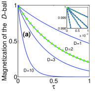
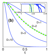
Figure 1: (Color online) Dynamics of $\mathcal{M}\left(t\right)$ from Eq. (2) integrated over the spatial dimensions for different initial conditions: (a) $m\left(\mathbf{x},0\right)=R_{0}^{D}/V_{D}\left(R_{0}\right)$; (b) $m\left(\mathbf{x},0\right)=R_{0}^{D}\delta\left(\mathbf{x}\right)$. Solid (blue) curves shows results from the $D$-dimensional radial random walk. For the two-dimensional case ($D=2$), we also plot the Dini-series of Eqs. (6) in (a) and (7) in (b) with (green) dots. Inset of (a) shows the short-time asymptotes of Eq. (5), dashed (green) lines. Inset of (b) shows the first-arrival times $\left\langle t_{1,N}\right\rangle$ (see text) with dashed vertical lines.

In Fig. 1 (a) we show the agreement between numerical results from the radial random walk for $D=2$ and the analytic solution of Eq. (6). Physical parameters have been set to unity besides $T_{V}\rightarrow\infty$, which means that we have no volume relaxation. We used $\Delta r=10^{-2}R_{0}$ and $10^{6}$ initial trajectories throughout where not explicitly stated.

II.2 Localised initial conditions

For an initially non-uniform magnetic moment the weight of higher modes are increasing and there is generally no short-time approximations available, as in Eq. (5). Motivated by this, we have in Fig. 1 (b) benchmarked numerical results also for the circle with opposite extreme initial conditions, the central delta spike $m\left(\mathbf{x},0\right)=R_{0}^{2}\delta\left(\mathbf{x}\right)$. In this case only the numerator in Eq. (6) change, and the total magnetization now reads

$$\mathcal{M}\left(t\right)=\mathcal{M}\left(0\right)e^{-t/T_{V}}\sum_{k=1}^{\infty}\frac{2\gamma_{k,0}J_{1}\left(\gamma_{k,0}\right)}{\left(\rho_{0}^{2}+\gamma_{k,0}^{2}\right)J_{0}^{2}\left(\gamma_{k,0}\right)}e^{-\gamma_{k,0}^{2}\tau},$$ (7)

and again agreement is found with the numerical results for $D=2$.

As seen in the inset of Fig. 1(b), the initial slope is zero because no walkers are initially close to the surface. The relevant quantity to predict is the time when the surface relaxation starts. If $p_{S}\sim 1$ it means that practically all trajectories are annihilated at the surface and we have a Dirichlet BC. For this case, we have confirmed that the time when the surface relaxation starts is precisely the first-arrival time $\left\langle t_{1,N}\right\rangle$. We plot the results of a second-order expansion of $\left\langle t_{1,N}\right\rangle$ YustePRE2001 in the inset of Fig. 1(b), from which qualitative agreement is observed even though $p_{S}\ll 1$ in those numerical examples. In comparison, the $j$th-first-arrivals time $\left\langle t_{j,N}\right\rangle$ YustePRE2001 for $j\simeq 1/p_{S}$ overestimates this time since early boundary arrivers may bounce close to the surface.

III The $D$-cube as a testcase for a Cartesian random walk

As the second basic domain, $\Omega$ is chosen to be the $D$-cube, and then it is straightforward to obtain a compact analytic solution for the magnetization valid for any $D$ with Sturm-Liouville theory from Eq. (2)

$$\mathcal{M}\left(t\right)=\mathcal{M}\left(0\right)e^{-t/T_{V}}2^{D}\prod_{j=1}^{D}\sum_{k_{j}=1}^{\infty}c_{k_{j}}e^{-\lambda_{k_{j}}\tau},$$ (8)

with coefficients

$$c_{k_{j}}=\left[\frac{\sin\left(\sqrt{\lambda_{k_{j}}}\right)}{\sqrt{\lambda_{k_{j}}}}\right]^{q}\frac{\sin\left(\sqrt{\lambda_{k_{j}}}\right)}{\cos\left(\sqrt{\lambda_{k_{j}}}\right)\sin\left(\sqrt{\lambda_{k_{j}}}\right)+\sqrt{\lambda_{k_{j}}}},$$ (9)

where $q=1$ ($0$) for uniform (central) initial conditions, while the eigenvalues $\lambda_{k_{j}}$ fulfill $\sqrt{\lambda_{k_{j}}}\tan\sqrt{\lambda_{k_{j}}}=\rho_{0}$.

We remark that for $D=1$, Eqs. (8) and (9) agrees with the $D=1$ result of the radial random walk of Eq. (4) with the physical domain being $r\in\left[-R_{0},R_{0}\right]$.

In agreement with Eq. (5), we can obtain from Eqs. (8) and (9)

$$\frac{1}{\mathcal{M}\left(0\right)}\left.\frac{d\mathcal{M}\left(t\right)}{dt}\right|_{t=0}=-2^{D}\prod_{j=1}^{D}\sum_{k_{j}=1}^{\infty}c_{k_{j}}\lambda_{k_{j}}=-\frac{\rho_{0}D}{R_{0}},$$ (10)

also for the $D$-cube. In fact the asymptotic results of Eqs. (5) and (10), for the specific geometries presented are generally valid for any connected pore in $D$ dimensions with a uniform initial condition. Integrating the dimensionless diffusion equation in Eq. (2) over the volume, applying the corresponding Robin BC, and finally using Gauss’s theorem for the divergence we have

$$\int\frac{\partial m}{\partial\tau}dV=-\rho_{0}\oint mdS=-\frac{\rho_{0}S}{V},$$ (11)

where we have assumed a uniform magnetic moment for all times, i.e., $m\left(\mathbf{x},\tau\right)=m\left(\tau\right)$, in the last step. The result (11) is in agreement with the right hand side of Eqs. (5) and (10) for the $D$-ball and $D$-cube respectively. Note that for fast diffusion (in relation also to the size and connectedness of the pores) the magnetic moment is kept approximately uniform and $\mathcal{M}\left(t\right)\sim\exp\left(-\rho St/V\right)$ for any time. Many estimates using the pore-size distribution are based on this approximation Kenyon1992 ; Cohen1982 ; MendelsonPRB1990 .

We now consider a random walk in a $D$-dimensional Cartesian lattice for a general porous medium. The change in the fraction of trajectories at a given lattice point during a time step $\Delta t$ is given by the probability for a step from any of the $2D$ neighboring lattice points, and then the probability for a step to the neighboring points is subtracted. For a point next to a boundary, that has $n$ neighboring boundary surfaces, we can without loss of generality for the result assume those to be in the positive Cartesian directions $x_{j},\>j=D-n+1,...,D$. We consider the change per time $\Delta t$ (with $\Delta r\equiv\Delta x_{1}=...=\Delta x_{D}$ for notational simplicity)

$$\frac{M\left(\mathbf{x},t+\Delta t\right)-M\left(\mathbf{x},t\right)}{\Delta t}=\frac{\Delta r^{2}}{2D\Delta t}\sum_{j=1}^{D-n}\left[\frac{M\left(\mathbf{x}-\Delta r\mathbf{e}_{j},t\right)-2M\left(\mathbf{x},t\right)+M\left(\mathbf{x}+\Delta r\mathbf{e}_{j},t\right)}{\Delta r^{2}}\right]$$

$$+\frac{\Delta r}{2D\Delta t}\sum_{j=D-n+1}^{D}\left[\frac{M\left(\mathbf{x}-\Delta r\mathbf{e}_{j},t\right)-M\left(\mathbf{x},t\right)}{\Delta r}\right]-\frac{1}{\Delta t}\frac{np_{S}}{2D}M\left(\mathbf{x},t\right)-\frac{p_{V}\left(\Delta t\right)}{\Delta t}M\left(\mathbf{x},t\right).$$ (12)

The second to last term in the above two-line single equation represents the $n$ paths to surface relaxation with probability $p_{S}$, and $p_{V}$ is the probability per time for volume relaxation. Multiplying Eq. (12) with $\Delta r$, and then neglecting all but the leading terms gives

$$0=\sum_{j=D-n+1}^{D}\left[\frac{\Delta r^{2}}{2D\Delta t}\frac{M\left(\mathbf{x}-\Delta r\mathbf{e}_{j},t\right)-M\left(\mathbf{x},t\right)}{\Delta r}-\frac{\Delta r}{\Delta t}\frac{p_{S}}{2D}M\left(\mathbf{x},t\right)\right].$$ (13)

Taking the limits $\Delta r\rightarrow 0,\>\Delta t\rightarrow 0$ (and $p_{S}\rightarrow 0,\>p_{V}\rightarrow 0$), with $\Delta t/p_{V}=T_{V}$ and $\Delta r^{2}/\left(2D\Delta t\right)=D_{0}$ constant, we have above the Robin boundary condition of Eq. (1) in each of the $n$ directions $x_{j},\>j=D-n+1,...,D$, with the identifications $D_{0}=\Delta r^{2}/\left(2D\Delta t\right)$ and $\rho=\Delta rp_{S}/\left(2D\Delta t\right)$. Hence, combining these two relations we have established the following surface relaxation relation for the BC in each of the $n$ directions,

$$p_{S}=\Delta r\rho/D_{0}.$$ (14)

This leading order relation is not novel MendelsonPRB1990 , and the higher order relation $\tilde{p_{S}}=\Delta r\rho/\left(D_{0}+\Delta r\rho\right)\simeq\sum_{j\geq 1}\left(-1\right)^{j+1}\left(\Delta r\rho/D_{0}\right)^{j}$ have been suggested BanavarPRL1987 . For $\Delta r\rho\ll 1$ the two relations $p_{S}$ and $\tilde{p_{S}}$ are practically equivalent, but the latter perform slightly better when benchmarked against the analytic result of Eq. (8) for large $\rho$ (we used $\Delta r=10^{-3}R_{0}$ for these tests).

Finally we note that several researchers apply an additional “factor $3/2$” in the surface relaxation relation (14) for arbitrary digital domains, as was derived in BergmannPRE1995 in $D=3$ for continuous random walks.

IV Local boundary conditions for digital domains

For random walk simulations to converge with high accuracy, the number of trajectories needs to be large, and the step-size ($\Delta r$) needs to be small, see FinjordTPM2007 ; Feller1967 for details. However, as we illustrate here for digitized media, the way the true geometry is mapped onto for example a computed tomography (CT) digital image is of additional importance. This is an intrinsic uncertainty, even if errors due to segmentation Mueter2012 and resolution are neglected.

We now introduce a correction factor $g\left(\mathbf{x}\right)$, to be multiplied with the right hand side of the surface relaxation relation in Eq. (14), for an improved local Robin boundary condition. With local we mean a local interpolated surface, even though for example $\rho$ can locally also depend on space and time. Clearly $g\equiv 1$ corresponds to no correction, while an exact local value of $g\left(\mathbf{x}\right)$ requires that we know the exact surface locally. This is not the case for a general digital image from an application, but we here use two basic domains to evaluate the presented method. In particular we have implemented a linear local boundary condition (LLBC) for the discrete Cartesian random walk for which a linear interpolation of a general digital surface is implicit but no knowledge about the true surface is required. More sophisticated correction factors, i.e., non-linear local boundary conditions corresponding to higher order interpolated surfaces, are possible. They may be motivated in future simulations if the input physical parameters are well known and high accuracy is required. However, we have concluded by the comparisons with the analytic solutions for the basic domains that already the LLBC correct a substantial part of the error in the dynamics caused by the digital misrepresentation.

As one way to evaluate the introduced local correction factor $g\left(\mathbf{x}\right)$ we introduce, motivated by Eqs. (5), (10) and (11), an initial slope which also depends on the orientation of the Cartesian coordinate system

$$\frac{1}{\mathcal{M}\left(0\right)}\left.\frac{d\mathcal{M}\left(t,\phi_{1},...,\phi_{D(D-1)/2}\right)}{dt}\right|_{t=0}\equiv-f\rho\frac{S}{V},$$ (15)

where $f\left(\phi_{1},...,\phi_{D(D-1)/2}\right)$ is defined above as a dimensionless global error factor dependent on the Euler angles in $D$-dimensions. The error factor $f$ can quantify the error in the initial slope of the total magnetization caused by the digital misrepresentation for a uniform initial condition of the magnetic moment. Note that the error factor $f$ is generally related to the correction factor $g\left(\mathbf{x}\right)$ in a non-trivial way.

V Results for linear local boundary conditions

We present results only for $D=2$ here, while LLBC in higher dimensions is considered and numerically applied to true CT-images of porous media in an ongoing research project.

  

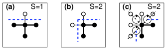
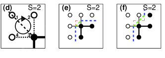
Figure 2: (Color online) Illustration of some pore-matrix interfaces for $D=2$. (a) One of the $4$ configurations for the number of neighboring surface (dashed lines) being $S=1$. (b) One of the $6$ configurations for $S=2$. (c) Neighboring cells needed to construct the LLBC for the case in (b). (d) A LLBC-diagram illustrating the four lattice points “1”, “2”, “3”, “4” (see text) in one of the cells. In (e), corresponding to (b), and in (f) we show examples of two different interpolated surfaces for $S=2$, e.g., in (f), $p_{S}$ for a step upwards (to the left) is reduced by a factor $1/\sqrt{2}\simeq 0.707$ ($\sqrt{2}/4+1/2\simeq 0.854$).

In order to construct LLBC around a point $\mathbf{x}$ we need to distinguish between the $2^{2^{D}}$ possible lattice configurations in each cell surrounding $\mathbf{x}$ in each diagonal direction that is in contact with a boundary, see Figs. 2(c) and (d). For this purpose we can locally define the integer $I\left(\mathbf{x}\right)=\sum_{j=1}^{2^{D}}Z_{j}2^{\left(2^{D}-j\right)}$, which for $D=2$ represents the $16$ different configurations $I\left(\mathbf{x}\right)\in\left\{0,1,...,15\right\}$, where $Z_{j}$ is chosen to be $1$ ($0$) for a lattice point inside (outside) the pore volume, i.e., in Fig. 2(d) for a black (white) dot around the point $\mathbf{x}$. If $I\left(\mathbf{x}\right)\in\left\{1,2,4,7,8,11,13,14\right\}$, it means that for any of these $8$ configurations we are locally going to interpolate a corner, see Figs. 2(b) and (e), for which we define the linear correction factor $g\left(\mathbf{x}\right)=1/\sqrt{2}$ (else $1$). Note that only half of the upper-left cell surface belongs to the move-up boundary, whereas half belongs to the move-left boundary, consider the diagonal lines in Figs. 2(c) and (d). The procedure we outline for locally generating these improved linear boundaries is equivalent to what is known in $D=3$ as Marching cubes, generalised to arbitrary dimensions in Bhaniramka2004 .

The two basic domains with the random walks presented in sections II and III respectively, are trivial in the sense that there are no local variations for the ratio of the true pore surface and the digitized surface (except the corners of the square in the Cartesian case). For simplicity, we then use $g\left(\mathbf{x}\right)=g=1/f$, i.e., with no space dependence, for a first numerical evaluation of the Cartesian random walk applied to the $D$-ball (for $D=2,3$), see Fig. 3.

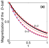
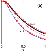
Figure 3: (Color online) Dynamics of $\mathcal{M}\left(t\right)$ for different initial conditions as in Fig. 1. Solid (blue) curves still shows results from the $D$-dimensional radial random walk for reference. Open (red) rings shows results from the Cartesian random walk in a digitized circle/sphere with $g=1/f$ (see text). For the circle ($D=2$) the results of using LLBC (see text) is shown with thick (black) curves slightly below the $g=1/f_{c}$ results for $D=2$. Further below the thick LLBC curve is the uncorrected results ($g\equiv 1$) for the digitized circle, dashed (red) curves.

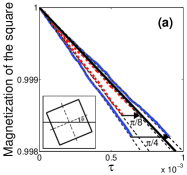
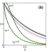
Figure 4: (Color online) LLBC improvements for a square with different orientations $\phi$, defined in the lower-left inset, are shown for small times in (a). Outer solid (blue) curves show numerical results for $\phi=\pi/4$, inner dashed (red) curves are for $\phi=\pi/8$. In both cases the most left curves are without LLBC ($g\equiv 1$), and the improvements by using LLBC are indicated with arrows pointing on the corrected curves. Thin dashed (black) lines shows analytic short-time asymptotes of Eq. (15) with $\rho S/V=2$ and (from left to right) the original error factors $f_{s}\left(\pi/4\right)=\sqrt{2}$, $f_{s}\left(\pi/8\right)\simeq 1.31$; respectively the error factors corresponding to LLBC: $f_{s}\left(\pi/8\right)\simeq 1.08$, $f_{s}\left(\pi/4\right)=1$, see text. The thick black curve is for an angle averaged LLBC with $\Delta\phi=\pi/160$. The corresponding full timeinterval to (a) is shown in (b) by the upper right family of curves, and with (green) dots for the analytic solution of Eq. (8). For the additional two $\rho_{0}=10$ (slow diffusion) lower curves only analytic solutions (green dots) and angle averaged LLBC (thick black) results are shown. Here the curve near $q=1$ is for $m\left(\mathbf{x},0\right)=1/4$ while $q=0$ corresponds to $m\left(\mathbf{x},0\right)=R_{0}^{2}\delta\left(\mathbf{x}\right)$.

For the remainder we concentrate the presentation on $D=2$. For the digitized circle ($c$) the surface is $8R_{0}$ (same for the square) and hence the digitized-to-true surface ratio gives the error factor $f_{c}=4/\pi\simeq 1.27$. After geometric considerations we obtained the corresponding LLBC ratio for the circle to be $f_{c}=8\left(\sqrt{2}-1\right)/\pi\simeq 1.05$. For the square ($s$), we illustrate the single angle variable $\phi$, i.e., $D(D-1)/2=1$ here, in the lower-left inset of Fig. 4. One can then show with geometry that the digitized-to-true surface ratio follows the $\pi/2$-periodic error factor $f_{s}\left(\phi\right)=\sqrt{2}\cos\left(\phi-\pi/4\right),\>0\leq\phi<\pi/2,\>f_{s}\left(\phi+\pi/2\right)=f_{s}\left(\phi\right)$, For the LLBC ratio one instead obtain the $\pi/4$-periodic error factor $f_{s}\left(\phi\right)=\sqrt{2}\left[\cos\left(\phi+\pi/4\right)+\sin\left(\phi\right)\right]$, with $\max(f_{s})=f_{s}\left(\pi/8\right)\simeq 1.08$.

To further minimize the risk of retrieving the worst case scenario in a simulation of an unknown digitized medium one can in principle examine all different orientations by varying the $D(D-1)/2$ Euler angles of the coordinate system. For the digitized square, a uniform average over the single Euler angle $\phi$ still overestimates the surface with $\langle f_{s}\rangle_{\phi}=f_{c}\simeq 1.27$, but only with $\langle f_{s}\rangle_{\phi}=f_{c}\simeq 1.05$ using LLBC.

The above results are strictly valid in the $\Delta r\rightarrow 0$ limit but showed good agreement with the numerical results that are presented in Fig. 4 for $\Delta r=10^{-2}R_{0}$.

VI Discussion and summary

While the LLBC can always be used, the exact correction factor can only be used if the true surface is known locally. However, for a complex porous medium where the variations of $\rho\left(\mathbf{x}\right)$ may also be partly unknown, a measurement of the total pore surface can then be useful. The initial slope from a NMR relaxation measurement probes a combined effect of $\rho\left(\mathbf{x}\right)$ and $S/V$, see Eq. (15), so measuring the surface-to-volume ratio can alone provide a first improvement. However, when comparing with measurements, keep in mind that a molecule carrying magnetic spin has a certain lengthscale (crossection) for surface relaxation, whereas for example common BET techniques Brunauer1938 maps out the surface dependent on the size of the molecule in use (e.g. $\sim 0.2$ nm for $N_{2}$).

Even when a correct (algorithm dependent) relation between $\rho$ and $p_{S}$ is used, the accuracy in diffusion simulations with Robin boundary conditions is severely restricted. This is due to an uncertainty of the true $\left(D-1\right)$-surfaces in a $D$-dimensional digitized media. As illustrated with the basic domains, the accuracy can be increased substantially by introducing a linear local correction to the relaxation on a digital surface. An improved interplay between experimental measurements and higher order algorithms for local Robin boundary conditions will increase the accuracy of simulations, applied to surface reactions and NMR dynamics in porous media and MRI-based analysis in medicine, beyond the first step taken here.

Finally we remark that local effects appears more dramatic if one for example directly study functions of $M\left(\mathbf{x},t\right)$ instead of its spatial integral.

References

- (1) F. Bloch, Phys. Rev. 70, 460 (1946).
- (2) H. C. Torrey, Phys. Rev. 104, 563 (1956).
- (3) I. T. Lin, H. C. Yang and J. H. Chen, Appl. Phys. Lett. 102, 063701 (2013).
- (4) E. O. Fridjonsson et al., Journal of Contaminant Hydrology 120-121, 79-88 (2011).
- (5) M. M. Tomadakis and T. J. Robertson, J. of Chem. Phys. 119, 1741 (2003).
- (6) W. E. Kenyon, Nucl. Geophys. 6, 153 (1992).
- (7) S. D. Senturia and J. D. Robinson, SPE J 10, 237 (1970).
- (8) M. H. Cohen and K. S. Mendelson, J. Appl. Phys. 53, 1127 (1982).
- (9) J. R. Banavar and L. M. Schwartz, Phys. Rev. Lett. 58, 1411 (1987).
- (10) K. J. Dunn, D. La Torraca and D. J. Bergman, Geophysics 64, 470 (1999).
- (11) P. E. Øren, F. Antonsen, H. G. Rueslåtten and S. Bakke, SPE 77398 (2002).
- (12) O. Talabi et al., Journal of Petroleum Science and Engineering 67, 168 (2009).
- (13) D. J. Bergman et al., Phys. Rev. E 51, 3393 (1995).
- (14) D. S. Grebenkov, Rev. Mod. Phys. 79, 1077 (2007).
- (15) K. R. Brownstein and C. E. Tarr, Phys. Rev. A 19, 2446 (1979).
- (16) Y. Q. Song, L. Zielinski and S. Ryu, Phys. Rev. Lett. 100, 248002 (2008).
- (17) J. Finjord et al., Transp. Porous Med. 69, 33 (2007).
- (18) C. H. Arns, T. AlGhamdi and J. Y. Arns, New J. of Phys. 13, 015004 (2011).
- (19) F. Hausser and E. Lakshtanov, Phys. Rev. E 86, 062601 (2012).
- (20) S. Boettcher and M. Moshe, Phys. Rev. Lett. 74, 2410 (1995).
- (21) S. B. Yuste, L. Acedo and K. Lindenberg, Phys. Rev. E 64, 052102 (2001).
- (22) K. S. Mendelson, Phys. Rev. B 41, 562 (1990).
- (23) W. Feller, An introduction to probability theory and its applications, Wiley, New York (1967).
- (24) D. Müter et al., Comp. and Geosc. 49, 131 (2012).
- (25) P. Bhaniramka, R. Wenger and R. Crawfis, IEEE Trans Visualization and Computer Graphics 10, 130 (2004).
- (26) S. Brunauer, P. H. Emmet and E. Teller, J. Am. Chem. Soc. 60, 309 (1938).