Monitoring Three-Dimensional Packings in Microgravity

Abstract

We present results from experiments with granular packings in three dimensions in microgravity as realized on parabolic flights. Two different techniques are employed to monitor the inside of the packings during compaction: (1) X-ray radiography is used to measure in transmission the integrated fluctuations of particle positions. (2) Stress-birefringence in three dimensions is applied to visualize the stresses inside the packing. The particle motions below the transition into an arrested packing are found to produce a well agitated state. At the transition, the particles lose their energy quite rapidly and form a stress network. With both methods, non-arrested particles (rattlers) can be identified. In particular, it is found that rattlers inside the arrested packing can be excited to appreciable dynamics by the rest-accelerations (g-jitter) during a parabolic flight without destroying the packings. At low rates of compaction, a regime of slow granular cooling is identified. The slow cooling extends over several seconds, is described well by a linear law, and terminates in a rapid final collapse of dynamics before complete arrest of the packing.

1 Introduction

Experiments with granular matter in microgravity allow access to regions in control-parameter space that are otherwise not accessible. Microgravity prevents the sedimentation of a loose non-agitated granular assembly and hence enables the long-term study of such states. For agitated granular matter, experiments in microgravity can reduce the inhomogeneity of driven states; and for particles in contact, the absence of gravity eliminates the pressure gradient in the packings. To what extent these goals can be realized in a specific experiment depends largely on the quality of the microgravity conditions found on specific platforms. Experiments have been performed for granular gases Falcon et al. (1999); Harth et al. (2013); Sack et al. (2013) as well as dense systems under shear Murdoch et al. (2013a, b). In the following sections, it will be shown how the microgravity environment of a parabolic flight can be utilized for investigating granular packings. Results will be elaborated for X-ray radiography as well as stress-birefringence in three dimensions.

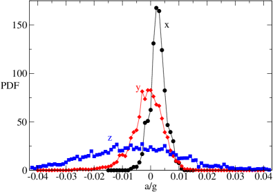
Figure 1: Distribution of rest accelerations averaged over a typical single parabola of 22 seconds on the third day of parabolic flight campaign DLR-22. Data are shown for the $x$- (circles, forward direction of the airplane), $y$- (diamonds, wing-to-wing direction of the airplane), and $z$-directions (squares, floor-to-ceiling direction of the airplane).

2 Microgravity

Microgravity environments are typically hard to obtain and require years of preparation. In contrast to experiments in space, parabolic flight campaigns offer a reasonably frequent opportunity to perform experiments under microgravity conditions. While not offering the best microgravity quality in terms of rest-accelerations, cf. discussion below, parabolic flights can help to test phenomena that depend on a distinction between top and bottom. One such phenomenon is convection. For a granular system under shear, convection was found perpendicular to the direction of shear along the direction of gravity Khosropour et al. (1997). On a parabolic flight however, it was observed recently, that in the absence of a distinction between top and bottom such convection disappears Murdoch et al. (2013a).

The limitation of such experiments on parabolic flights is the presence of rest-accelerations – called $g$-jitter – which drastically restrict the time the particles can stay in a granular gas without being collectively driven against the container walls within around a second. For dense granular matter, the $g$-jitter imposes a minimum necessary confinement for keeping granular packings confined.

Figure 1 shows the distribution of rest accelerations on a parabolic flight, averaged over a single flight day. The $x$-direction is defined from the tail to the front of the plane, the $y$-direction is from the left to the right wing when looking from the cabin to the cockpit, and the $z$-direction points from the floor to the ceiling of the cabin. Given the rather uncontrolled nature of the rest-accelerations, it is remarkable how well they follow reasonable distributions. The full width of the distributions at half maximum in units of $g$ is 0.005 for the $x$-direction, 0.01 for the $y$-direction, and 0.04 for the $z$-direction. In addition to the width of the distributions showing rather large qualitative differences, also the maximum values in $x$- and $z$-directions show deviations from zero, $a_{x}^{0}/g\approx 0.0025$ (forward bias) $a_{z}^{0}/g\approx-0.012$ (downward bias). The $y$-direction is on average symmetric. Data for a single parabola typically look similar to Fig. 1 while being somewhat variable between individual parabolas.

Rather than trying to avoid the influence of the rest-accelerations, in the following experiments the $g$-jitter is utilized for providing agitation for dense granular systems.

3 X-Ray Radiography

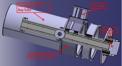
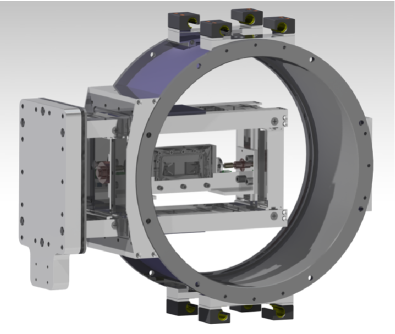
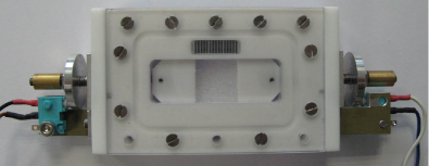
Figure 2: Experimental setup for the parabolic flight (DLR-22, April 2013) for X-ray radiography. The top panel shows a schematic view from left to right of the X-ray tube, the experiment chamber with sample cartridge, a spacer ring, and the detector. The central panel exhibits the sample chamber with the replaceable cartridge for granular experiments which is shown in the photograph of the bottom panel. The granular cartridge has two motorized pistons of cross-section 15mm$\times$5mm and an X-ray ruler with a mm-scale on top.

The use of X-ray illumination facilitates the visualization of otherwise optically opaque samples. The simplest use of a combination of an X-ray source and a detector is by recording the transmission images after absorption from the sample in a radiography setup. X-ray radiography has been used to investigate hopper flow of sand Baxter et al. (1989) as well as the dynamics of granular matter in fluidized beds Grohse (1955); Rowe and Everett (1972); Yates et al. (2002). The addition of tomography, i.e. rotating the still sample for multiple transmission images, allows the reconstruction of packings Aste (2006); Jerkins et al. (2008).

The aim of the present study using X-ray radiography is to investigate the compaction of a granular assembly into a dense packing. On ground the compaction is dominated by gravity-induced sedimentation and takes place rather rapidly within a fraction of a second and also comparably violently with shock waves traveling through the system Son et al. (2008). In microgravity, the energy loss is still driven by interparticle collision but the rapid sedimentation is replaced by the compaction from the container walls which is chosen here to be rather moderate in speed.

Figure 2 shows the setup of the radiography device. The source produces a divergent X-ray beam that irradiates a sample before being registered by the detector (CCD-/COOL-1100XR) with pixel size 9$\mu$m$\times$9$\mu$m recording with a resolution of 2008$\times$1340 pixels and 16-bit depth at 4 fps (frames per second). The placement of the sample between source and detector as well as their overall distance determines the magnification. Additional spacer rings can be used to increase the possible magnification. In the following, a magnification factor of 2 was chosen. The actual sample cell is placed in a sample chamber in the form of a replaceable cartridge. In addition to changing granular samples easily, also samples other than granular matter can be used with the device. As seen in the bottom panel of Fig. 2, the granular sample cell contains the sample material inside a rectangular volume that can be changed by pistons on two sides. An X-ray ruler with a millimeter scale is used to calibrate the volume and hence the packing fraction of the experiments.

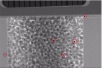
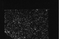
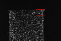
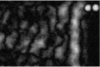
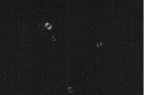
Figure 3: Radiography images from parabola number 1. The original transmission image (upper left) shows the pile of glass particles (diameter 500$\mu$m) in the 2-g phase before the microgravity experiment. Gravity acts perpendicular to the plane of the image. Darker particles singled out by red circles are steel particles (diameter 200$\mu$m) acting as tracers. The difference image (upper right) shows the motion between two successive frames due to g-jitter at the beginning of compaction (recording at four frames per second). A similar image (middle left) shows the differences immediately after motion of the pistons together with a rectangular frame for the enlarged selection shown on the next difference image (middle right). The fourth difference image (lower left) shows the absence of detectable motion after compaction and cooling of the arrested sample. The final difference image (lower right) illustrates the motion of four rattler particles at the transition from the 0g to the 2g-phase.

The device described above was used in the parabolic flight campaign DLR-22 in April 2013. The orientation of the X-ray beam was chosen in the $z$-direction of the airplane, so the largest dimensions of the sample cell were in the $x$-$y$-plane of the aircraft where the least overall bias of the $g$-jitter could be expected. The sample volume was filled with around 8000 glass particles of diameter 500$\mu$m (estimated coefficient of restitution $\varepsilon\approx 0.7$). Tracer particles of diameter 200$\mu$m were added to have access to individual particle trajectories. These particles were made from steel to ensure good contrast which is seen in the first panel of Fig. 3. The choice of tracer particles much smaller than the particles of the host system was motivated by the resolution limitations in both space and time: Smaller particles are more likely to be rattlers, i.e. show appreciable motion even inside an arrested state. The volume was filled with particles on ground and compacted with the pistons to form a stable packing without deforming the particles. Afterwards the pistons were retracted symmetrically and left the granular particles in a pile as seen in the upper left panel of Fig. 3 with more particles in the center than closer to the pistons. This asymmetry vanishes immediately after entering the microgravity phase where the $g$-jitter redistributes the particles homogeneously in the sample volume.

After agitation of the granular particles by $g$-jitter, the system was slowly compressed by the pistons from a packing fraction of around $\varphi=0.43$ until the arrested state around $\varphi=0.6$ was reached. The reported packing fractions are calculated from dividing the volume of the particles by the full available volume of the test cell. For the packed state we estimate the deviation of the true bulk packing fraction from the nominal one as follows: We subtract from the particle volume the sum of the half spheres of a completely covered layer of particles at the walls. From the cell volume we subtract the corresponding sum of half-cubes. The resulting boundary-corrected value for the packing fraction at the arrested state, $\varphi=0.6$, is found at $\tilde{\varphi}=0.615$, i.e. a deviation of 2.5% for the bulk value inside the sample. Since this correction is not reasonable for more dilute assemblies down to nominal packing fraction of 0.43, the nominal values are reported in the following. Even accounting for the outlined boundary correction, the arrested sample does not reach values for the packing fraction commonly reported for random-close packing of around $\varphi=0.64$. The lower packing fraction at the arrested state in our samples is explained by the comparably high friction among the particles.

The difference image in the upper right panel of Fig. 3 shows the absolute intensity variation from one frame to the successive one and hence characterizes the overall motion across the sample. It is found that the particles at the initial volume are quite well agitated. The volume of particles in that difference image is distinguished well from the container walls which do not move and appear black plus some noise. The middle panels of Fig. 3 show the motion immediately after compression by the pistons which is visible by the two trapped tracer particles on the lower-left and upper-right corners. While on the right wall a whole layer of particles is displaced together, on the left wall the energy input yields a more random pattern. This difference is not very surprising as the particle density at both walls is not necessarily the same before the particles are packed densely. A rectangular frame in the middle left panel indicates an area in the full test cell that is shown magnified by a factor of seven in the middle right panel. It is clear from the enlarged image that in the setup individual tracer particles can be resolved.

Once the final close-packed volume is reached, the motion in the sample cell vanishes as seen by the completely dark difference image in the lower left. Container and particle packing are then indistinguishable. The final difference image in Fig. 3 shows the observations at the transition from microgravity to 1.8$g$ at the end of a parabola: As both new and old position of a particle show up brightly, four individual particles can be identified as moving on the timescale of a quarter second. We interpret these as rattlers that have lost all their energy during cooling inside the packing and are now pulled downwards by the 2$g$ acceleration.

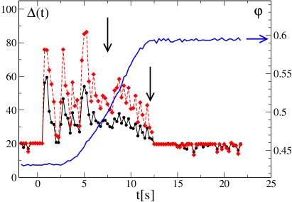
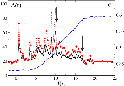
Figure 4: Dynamics of the granular particles during the slow compaction process. The plots display the overall brightness of successive difference images $\Delta(t)$ on the left axes over time during the microgravity phase for a representative compaction run within 10 seconds (parabola 10, upper panel) and a run within 13 seconds (parabola 1, lower panel). The respective right axes display the evolution of the packing fraction for the full curve. The two curves for $\Delta(t)$ show the average over the full sample (filled circles) and the center of the cell without boundaries (diamonds). Vertical arrows indicate a region of slow cooling (see text).

The time evolution of the brightness in the difference images can serve as an estimate of the granular system’s kinetic energy and hence the decrease in brightness signals granular cooling. This evolution of the brightness is shown in Fig. 4. The brightness of the difference images $\Delta(t)$ is defined by the averaged greyvalue per pixel over a region of interest. The region of interest is taken either for the entire probe-cell volume (with the trade-off of including the pistons for the later part of the compaction) shown as diamonds as well as over only the central quadratic region filled with particles after compaction without any boundaries shown by the filled circles (with the trade-off of missing some particles close to the walls at the earlier part). Both definitions of the region of interest yield no qualitative difference in the observed data, so it seems both definitions capture the particle dynamics reasonably well and the dynamical features are dominated by the behavior in the bulk. The origin of the time scale is set to the beginning of the 0$g$ phase. The compaction is seen by the evolution of the packing fraction over time. The overall packing fraction is reduced by $\Delta\varphi/\Delta t=0.017/s$ for compaction in 10s and by $\Delta\varphi/\Delta t=0.013/s$for compaction in 13s, respectively. For those slow compaction rates, data from 10 parabolas was used. Similar five runs have been obtained for a fast compaction rates of $\Delta\varphi/\Delta t=0.04/s$ which is not shown in the figure but discussed below.

For slow compaction, at both reported compaction rates the reproducible observations can be summarized as follows.

(1) Throughout all the runs, both for the beginning when particles are at rest in 1.8$g$ and at the end of compaction when still in a noisy 0$g$ environment, the background value is always $\Delta_{0}=20$. There is no observable drift in $\Delta_{0}$ and in the $\Delta(t)$ over different runs. Faster overall motion of the particles as apparent from the original images is reflected in a higher amplitude of $\Delta$.

(2) At the start of 0$g$, the system is shaken strongly and exhibits strong fluctuations in $\Delta(t)$ seen by the large peaks in both panels of Fig. 4 on the respective left sides. The fluctuations are not affected by the compaction which is setting in after a few seconds in 0$g$.

(3) Around $\varphi=0.5$ (indicated by vertical arrows in Fig. 4) fluctuations are dampened and the evolution of $\Delta(t)$ suggests a regime a granular cooling. This cooling regime was found for 10 out of 11 runs with slow compaction. For the single exception the pistons got stuck and snapped before a cooling regime can be identified in the data. A reminiscence of that stick-slip piston behavior can be seen around 10s in the lower panel of Fig. 4 in the curve for the packing fraction.

(4) The cooling regime shows up similarly for both definitions of a region of interest; the more restricted region of interest (diamonds) is used for the quantitative analysis in the following. The slow cooling can be described by a linear law $\Delta(t)-\Delta_{0}=\tilde{\Delta}\gamma t$ where $\tilde{\Delta}$ describes the overall amplitude, i.e. the equivalent of granular temperature, at the beginning of the cooling. For the amplitude we obtain $\tilde{\Delta}=40$ for the upper panel in Fig. 4 and $\tilde{\Delta}=30$ for the lower panel. Parameter $\gamma$ describes a normalized cooling rate that turns out to be well reproducible across all 10 parabolas for slow cooling with no significant difference for different compaction rates: $\gamma=0.13\pm 0.02/s$.

(5) The linear regime for slow cooling is terminated upon reaching the final packing fraction by a fast cooling regime where within around $1s$ the complete dynamics comes to rest, i.e. $\Delta(t)=\Delta_{0}$. The limited time resolution of the data does not allow a more quantitative statement, but the fast cooling regime is always identified clearly, the linear regime for slow cooling does not extend all the way to $\Delta_{0}$. After the fast cooling regime, the sample is arrested. Note that the appearance of rattlers as seen in Fig. 3 is not visible above the noise level in $\Delta(t)$.

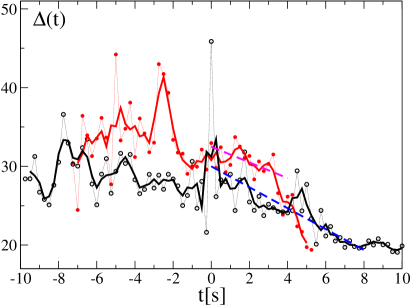
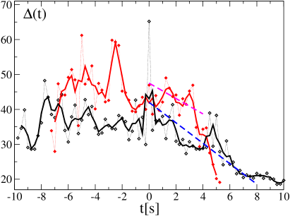
Figure 5: Averages over the particle dynamics during the slow compaction process evaluated for all pixels (top panel) and the selected region of pixels (bottom panel). The origin of time is set to the time when $\varphi=0.5$ for each run. The open symbols in both panels represent the average over parabolas P0 to P5 (compaction rate $\Delta\varphi/\Delta t=0.013/s$) while the full symbols show results from parabolas P6 to P10 (compaction rate $\Delta\varphi/\Delta t=0.017/s$). Full curves are corresponding running averages in time over 0.5s, i.e. the average of three data points. Dashed straight lines display the linear laws $\Delta(t)=\tilde{\Delta}\gamma t$.

Observations (1) to (5) as elaborated above are found for all realizations of slow compaction for 10 parabolas. In particular, the limit of $\varphi=0.5$ where fluctuations become smaller and cooling sets in, is reproducible across the available data. If the compaction is around four times faster as investigated for additional five parabolas, no such limit exists and no such regime of slow cooling can be identified. Also, in Fig. 4 one observes that the range of validity for the linear law shrinks from 6.5s for compaction rate $\Delta\varphi/\Delta t=0.013/s$ to 4.5s for $\Delta\varphi/\Delta t=0.017/s$. Hence, we conclude that the existence of a slow cooling regime depends on the balance between energy input (from $g$-jitter and the compaction process) and the rate of dissipation (given by $\varepsilon$) and can be tuned by the rate of compaction. For fast enough compaction, the slow cooling regime vanishes.

The averages of the cooling dynamics for all available data from the parabolic flight are shown in Fig. 5. For the small compaction rate $\Delta\varphi/\Delta t=0.013/s$, data from parabolas P0, P1 (cf. lower panel in Fig. 4), P2, P3, P4, and P5 are first rescaled in time to overlap in the evolution regarding the packing fraction $\varphi$ with $\varphi=0.5$ chosen as $t=0$. Then the data for $\Delta(t)$ is averaged over the 6 data sets and shown for the full range of pixels as open circles (upper panel of Fig. 5) as well as open diamonds (lower panel of Fig. 5). Running averages in time are used to obtain the somewhat smoother corresponding full curves. Data for compaction rate $\Delta\varphi/\Delta t=0.017/s$ is treated similarly and displayed as filled circles (upper panel) and filled diamonds (lower panel). From the averaged dynamics, linear cooling laws can be obtained that are consistent with the results from the single runs described above: Compaction rate $0.013/s$ is described by $\Delta(t)-\Delta_{0}=10-1.33t$ while compaction rate $0.017/s$ follows $\Delta(t)-\Delta_{0}=12.5-t$ in the upper panel. The different slopes in those laws follow the variation of the overall amplitude of $\Delta(t)$ varies by around 25%. In the lower panel the corresponding laws read $\Delta(t)-\Delta_{0}=2.2(10-1.33t)$ and $\Delta(t)-\Delta_{0}=2.2(12.5-t)$, respectively. Hence, the limitation to the pixels in the selected region only introduces an additional amplitude.

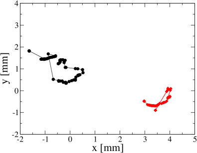
Figure 6: Trajectories of two tracer particles ($d=200\mu$m) inside an assembly of host particles ($d=500\mu$m) during compaction in microgravity (parabola 3 on day 3 of DLR-22).

The linear law is valid for around 4s for $\Delta\varphi/\Delta t=0.017/s$ and for 8s for the compaction rate $0.013/s$ which may be accidental. Also for the averaged data, the slow linear cooling is followed by a more rapid decay of $\Delta(t)$. Again, the final rapid collapse takes place within a second and it is observed in Fig. 5 that the final decays may be scaled on top of each other for different compaction rates. It is possible to interpret the data for different compaction rates by a roughly constant decay rate $\gamma$ and a shrinking range of validity in time after which the final collapse terminates the slow cooling. The fits of the individual decay curves for $\Delta(t)$, cf. Fig. 4, yield such a constant $\gamma$ when averaged. It is also possible to imagine that the cooling regime vanishes by a decreasing slope $\gamma$ whereby the increased energy input at higher compaction rates can overcompensate for the dissipation. The latter scenario is consistent with the finding that in the fits of the averaged $\Delta(t)$ in Fig. 5, a slight decrease in the value of $\gamma$ is obtained.

While the overall motion can be estimated from the difference images, the tracer particles are visible in the transmission images and can be tracked individually. Figure 6 shows the trajectories of two tracer particles during the compaction run shown in Fig. 3. While the data are not sufficient to properly define a diffusion coefficient, it is seen that despite the relatively high density the tracers travel over distances several times their own diameter. Interestingly, the particle closer to the center of the cell moves over a larger distance than the particle closer to the right piston. However, since the motion in the perpendicular direction is not know, no final conclusion can be drawn.

4 Stress Birefringence in Three Dimensions

The first investigation using stress-birefringent particles to model the stress transmission in granular packings was done by Dantu (Kuske and Robertson, 1974, p. 500ff). In two dimensions, Pyrex glass cylinders were viewed between crossed polarizers exhibiting chains of larger stresses when penetrated with a piston. In three dimensions, crushed and sieved Pyrex glass particles were immersed in an index-matching liquid, allowing a view inside the sample also showing stress chains between crossed polarizers. Later, the existence of stress chains in three dimensions was also demonstrated and analyzed with spherical glass beads Liu et al. (1995); Wood and Leśniewska (2011).

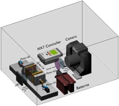
Figure 7: Experimental setup for the parabolic flight (DLR-13, February 2009) for stress measurements. Stress-birefringent particles inside a sample cell with cross section 5cm$\times$5cm and two pistons movable by motors 1 and 2 are illuminated by an LED panel from behind and recorded between crossed polarizers by a camera. Compression and recording is operated by an NXT controller and initiated from outside via a bluetooth signal from a cell phone. The entire setup is enclosed in an aluminium box, weighs 10kg in total, and is left free-floating for distances up to 50cm inside the cabin.

While for three dimensions, granular stress-birefringence has so far remained largely on the qualitative level, in two dimensions, granular stress-birefringence (also called photoelasticity) has been utilized in a large variety of instances and analyzed in great detail: In sheared systems the transition between loose and load-carrying packings was established Howell et al. (1999); a qualitative difference in force response to external loads was found for ordered and disordered packings Geng et al. (2001); logarithmic aging of stress was discovered for packings but not observed under compression Hartley and Behringer (2003); the relation between force chains and friction in stick-slip motion was elaborated Yu and Behringer (2005); for granular sound, the propagation along force chains was demonstrated Owens and Daniels (2011); for jamming under isotropic compression, non-trivial power-laws were confirmed Majmudar et al. (2007); Behringer et al. (2008); Zhang et al. (2009) and distinguished from jamming behavior under shear Majmudar and Behringer (2005); Utter and Behringer (2008); Zhang et al. (2010); Bi et al. (2011).

The investigation of granular stress-birefringence in two dimensions continues to be a fruitful route for detailed analysis of the statistical properties of granular packings as well as its dynamical properties. Motivated by this success, we attempt to extend the methods towards three dimensions in the following. Figure 7 shows the setup of the granular compaction experiment for the parabolic flight campaign DLR-13 in 2009. The sample cell containing the granular particles is illuminated from behind by an LED panel which has a polarizer laminated on top of it. A rotatable quarter-wave plate in addition to a polarizer in front of a camera (Nikon D3) completes the polariscope. Pistons at two walls of the sample cell can be moved by servo motors to change the volume and allow for the compaction of the granular particles from a loose assembly into a force-carrying packing. The switching of illumination, the motion of the motors, the rotation of the quarter-wave plate, and the multiple release of the camera is fully automated by an NXT controller. The experiment box is left floating freely for up to 50cm inside the plane. Measurements are performed during the 0g-phase of the parabolic flight and in order to minimize the disturbance, the start of the measurement is triggered from the outside by a cell phone (Nokia 6131) via bluetooth.

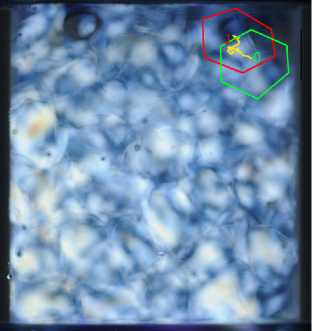
Figure 8: Rattler motion observed against the force-network backbone visualized by stress-birefringence. The outlines indicate the rattler at its initial (0, green) and end (1, red) position. The path (yellow) shows the distance traveled.

Since glass has a very small stress-optical coefficient, high external pressures (of the order of several 100kPa) are needed to obtain an appreciable signal from a packing of glass particles. In contrast, the present experiments are performed with gelatine particles in a water-glycerol mixture for index-matching. While gelatine has been used for photoelastic investigations (see Kuske and Robertson (1974) for a review) the production of stress-free particles needed to be refined and shall be detailed elsewhere. The use of gelatine reduces the demand on the mechanical structures of the microgravity device and hence allows for easier implementation. Already below 100Pa, an assembly of gelatine particles exhibits a reliable signal. In addition, one can approach much closer the transition point where the granular particles lose or establish contacts. In order to prevent ordering for particles of the same size, irregular particles are cast with a mean diameter of around 9mm with a shape indicated by the outlines in Fig. 8.

The state of a partially index-matched sample of irregular particles is shown in Fig. 8 after compaction from left and right with the pistons of cross section 5cm$\times$5cm. The corresponding motion of the ratter particle after compaction in microgravity is demonstrated in the movie 0g-rt.mpg in the supplementary material. The color fringes reveal the existence and inhomogeneity of the stresses inside the force network in the sample. The dark sphere at the upper left end of the picture is an air bubble. The partial index match allows for the simultaneous observation of particle motion and it is found that among around 300 particles only a single particle in the front upper right corner is still moving. The trajectory of the particle’s center is similar to the motion of the tracers in the X-ray experiment, cf. Fig. 3. The distance traveled by the rattler is about half its diameter. The differences in the shapes of the outline in the beginning and the end of the trajectory are due to the rotation of the rattler in its pocket formed by the arrested particles.

5 Conclusion

It has been shown that X-ray radiography and stress-birefringence allow the observation of the compaction of a granular packing in microgravity. Remarkably, the conditions on parabolic flights are especially suitable to observe rattlers that are agitated by the rest-accelerations without destroying the packings. Both methods can identify reliably the motion of a small fraction of rattler particles among the network of particles that form the backbone of the packing. While not enough data is currently available for an elaborate analysis of rattler dynamics from 3D stress-birefringence or the tracer dynamics in X-ray radiography, the results show nevertheless that microgravity experiments give access to new phenomena not observable on ground.

For the X-ray radiography data it is possible to quantify the bulk dynamics in the samples, resulting in much more reliable statistics. Using the time gradient by analyzing the difference images from the detector, a reliable quantity $\Delta(t)$ can be obtained to characterize the motion of the particles. $\Delta(t)$ allows the distinction between agitated and arrested states. In addition, it is possible to identify a novel regime of cooling quantitatively for low rates of compaction. This is only possible in microgravity as under the dominating influence of gravity granular gases collapse quite rapidly Son et al. (2008). The newly identified cooling extends over several seconds and is described reasonably well by a linear decay of $\Delta(t)$.