Using Web Co-occurrence Statistics for Improving Image Categorization

Abstract

Object recognition and localization are important tasks in computer vision. The focus of this work is the incorporation of contextual information in order to improve object recognition and localization. For instance, it is natural to expect not to see an elephant to appear in the middle of an ocean. We consider a simple approach to encapsulate such common sense knowledge using co-occurrence statistics from web documents. By merely counting the number of times nouns (such as elephants, sharks, oceans, etc.) co-occur in web documents, we obtain a good estimate of expected co-occurrences in visual data. We then cast the problem of combining textual co-occurrence statistics with the predictions of image-based classifiers as an optimization problem. The resulting optimization problem serves as a surrogate for our inference procedure. Albeit the simplicity of the resulting optimization problem, it is effective in improving both recognition and localization accuracy. Concretely, we observe significant improvements in recognition and localization rates for both ImageNet Detection 2012 and Sun 2012 datasets.

1 Introduction

Object recognition from images is a challenging task at the intersection of computer vision and machine learning. A major source of difficulty stems from the fact that the number of object classes is large and it is easy to confuse visually related objects. The bulk of the work on object recognition focused on the task of identifying individual objects from a single or multiple patches of the image. The existence of semantically related objects in a single image is often sidestepped, though as the number of object classes increases the potential of class confusion dramatically increases as well.

Few approaches were proposed in the computer vision literature to incorporate contextual information, see for instance [4, 11, 12]. Existing object classification methods that incorporate context fall roughly into two categories. The first considers global image features to be the source of context, thus trying to capture class-specific features [12]. The second classifies objects while taking into account the existence of the rest of the objects in the scene [11]. The latter work used Google Sets as a source of information for co-occurrences of objects. Unfortunately this source of information was inferior to using co-occurrence information gathered from image training data. Research in the second setting has further generalized in various ways. The work of Galleguillos et al. [4] considers both semantic context, that is, co-occurrences of objects as well as spatial relations between objects. In [1], the authors further extend the latter approach by proposing an “Object Relation Network” that models behavioral relations between objects in images. The aforementioned approaches typically require laborious localization and labeling of objects in training images. To mitigate this problem, the usage of unlabeled data through grouping of image regions of the same context was proposed in [5].

In this paper we present an approach that infuses an external information source that captures the statistical tendency of visual objects to co-occur in images. Rather than resorting to the image content itself for the co-occurrence model, we use a large collection of textual data to count the co-occurrences for any set of objects, as illustrated in Figure 1.

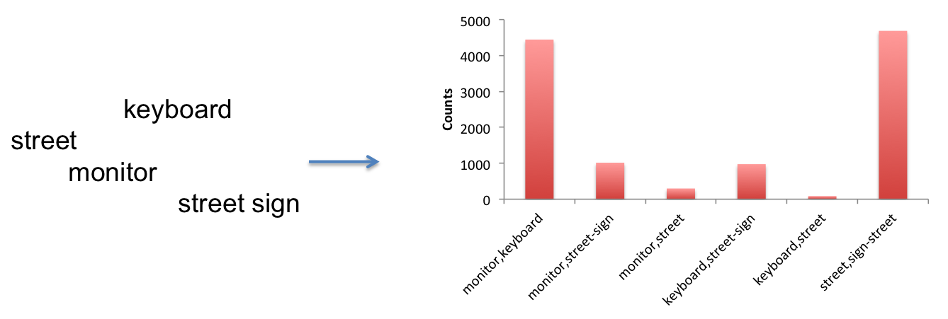
Figure 1: Results of co-occurrence counts for a set of indoor and outdoor object pairs. The counts are computed from a small corpus of text documents on the Web. Large counts correspond to object-pairs that often co-occur together. It can be seen that objects found indoor also tend to co-occur in text and similar behavior is observed for outdoor objects. For example, monitor and keyboard have a high chance to appear together in a text document while monitor and street do not. This suggests that text co-occurrence is significantly correlated with visual co-occurrence. Exploiting this fact is one of the contributions of this paper.

As mentioned above, most of prior work, including the cited papers, is built upon the visual training set itself. To our knowledge, there was not a substantial effort to incorporate external information from vastly different information sources, such as web documents that is considered in this paper. In contrast, modern speech recognition approaches have been using language models for many years [10]. In speech recognition systems, the acoustic model is trained to recognize individual or short sequences of phonemes. Its output is used by a “decoder” that incorporates language statistics, typically in the form of a Markovian model whose parameters are estimated from heterogeneous text sources. We propose to use an analogous (yet simpler) approach for performing multiple object recognition. While images do not exhibit the rich morphological and syntactic structure of natural languages, we show that the co-existence of semantically related objects can still be leveraged. Our approach indeed draws a parallel line to speech recognition systems in which the acoustic model is combined with a language model that is typically constructed from text-based sources. However, due to the lack of temporal structure our decoding procedure diverges from the dynamic-programming and cast the inference task as a static optimization problem.

The end result is a general and scalable scheme that can be applied to different sources of images while incorporating the statistical co-occurrence model without the need of specialized training data. We term our approach Laconic as an acronym for label consistency for image categorization.

The rest of the paper is structured as follows. Sec. 2 describes the Laconic model and the underlying optimization that is used as an inference tool. Sec. 3 describes the co-occurrence model and how it is estimated from the web. Sec. 4 presents experimental results on two different datasets (Sun12 and ImageNet) for which significant performance improvements are shown when using Laconic. Finally, some conclusions and potential extensions are provided in Sec. 5.

2 The Laconic Setting

We start by establishing the notation used throughout the paper. We denote scalars by lower case letters, vectors by boldface lower case letters, e.g. $\boldsymbol{v}\in\mathbb{R}^{p}$, and matrices by upper case letters. The transpose of a matrix $A$ is denoted $A^{\mbox{T}}$. Vectors are also viewed as $p\times 1$ matrices. Hence, the $2$-norm squared of a vector can be denoted as $\boldsymbol{v}^{\mbox{T}}\boldsymbol{v}$. We denote the number of different object classes by $p$.

The Laconic objective consists of three components: an image-based object score which is obtained from an image classifier (see Sec. 4), a co-occurrence score based on term proximity in text-based web data (see Sec. 3), and a regularization term to prevent overfitting. We denote the vector of object scores by $\boldsymbol{\mu}\in\mathbb{R}^{p}$ where the value of $\mu_{j}$ increases with the likelihood that object $j$ appears in the image. We refer to this vector as the external field. We denote the matrix of co-occurrence statistics or object pairwise similarity by $S\in\mathbb{R}_{+}^{p\times p}$. This matrix is highly sparse and its entries are non-negative. Its construction is described in Sec. 3. We also optionally add domain constraints on the set of admissible solutions in order to extract semantics from the scores inferred for each label and as an additional mechanism to guard against overfitting.

Abstractly, our inference amounts to finding a vector $\boldsymbol{\alpha}\in\mathbb{R}^{p}$ minimizing the following objective,

$${\cal Q}(\boldsymbol{\alpha}|\boldsymbol{\mu},S)={\cal E}(\boldsymbol{\alpha}|\boldsymbol{\mu})+\lambda{\cal C}(\boldsymbol{\alpha}|S)+\epsilon{\cal R}(\boldsymbol{\alpha})~{}~{}\mbox{s.t.}~{}~{}\boldsymbol{\alpha}\in\Omega~{},$$ (1)

where $\lambda$ and $\epsilon$ are hyper-parameters to be selected on a separate validation set. For concreteness we describe the inference procedure as a minimization task. The first term ${\cal E}(\boldsymbol{\alpha}|\boldsymbol{\mu})$ measures the conformity of the inferred vector $\boldsymbol{\alpha}$ to the external field $\boldsymbol{\mu}$. We tested the following terms

$$-\boldsymbol{\mu}^{\mbox{T}}\boldsymbol{\alpha}$$ [linear] (2)

$$\sum_{j=1}^{p}\alpha_{j}\log\left(\frac{\alpha_{j}}{\mu_{j}}\right)+\mu_{j}-\alpha_{j} \mbox{[relative entropy]}~{}.$$ (3)

The linear score can be used in all settings, in particular, when the outputs of the object recognizers take general values in $\mathbb{R}^{p}$. The relative entropy score can be used when the outputs are non-negative, especially in the case where the outputs are normalized to reside in the probability simplex. Such normalization often takes place by applying a softmax function at the top layer of a neural network.

Shifting our focus to the second term ${\cal C}(\boldsymbol{\alpha}|S)$, we experimented with the following scores,

$$-\boldsymbol{\alpha}^{\mbox{T}}S\boldsymbol{\alpha}$$ [Ising] (4)

$$\sum_{i,j}{S}_{i,j}\,{\cal D}(\alpha_{i}-\alpha_{j}) \mbox{[difference]}~{}.$$ (5)

The Ising model assesses similarity between activation levels of object category pairs. When $S_{i,j}$ is high, the two categories tend to co-occur in natural texts underscoring the potential of similar co-occurrence in natural images. Thus, the value of $\alpha_{j}$ will be “pulled up” by $\alpha_{i}$ if the external field of the latter, $\mu_{i}$, is large. The sum of (4) and (2) is essentially the Ising model [7]. In contrast to the physical model, we do not require an integer solution. Alas, for general matrices $S$, the objective function ${\cal Q}$ is not convex in $\boldsymbol{\alpha}$. Thus, while we are able to use classical optimization techniques, a convergent sequence is likely to end in a local optimum. We revisit this issue in the sequel.

The divergence ${\cal D}:\mathbb{R}^{2}\rightarrow\mathbb{R}_{+}$ assesses the difference between the activation levels of two labels. Let $\delta$ denote the difference of an arbitrary pair $\alpha_{i}-\alpha_{j}$. We evaluated and experimented with several options for ${\cal D}$, based on $\ell_{p}$ norms and the Huber loss. We report result for the Huber loss, defined as,

$${\cal D}_{\mbox{H}}(\delta)=\left\{\begin{array}[]{ll}\delta^{2}/2&|\delta|\leq 1\\ (|\delta|-1/2)&|\delta|>1\end{array}\right.~{}.$$ (6)

All the difference-based penalties we constructed are convex in $\boldsymbol{\alpha}$. However, difference-based penalties inhibit the activation values of objects that tend to co-occur frequently in texts to become vastly different from each other. This property while seemingly useful is in fact a two-edged sword as it may create “hallucination” artifacts when solely one of two highly-correlated labels appears in an image. Indeed, as our experimental results indicate, by using multiple random starting points, the Ising-like penalty yields better retrieval performance.

Finally, we need to describe the regularization component and the domain constraints. Throughout our experiments we incorporated a $2$-norm regularization, namely ${\cal R}(\boldsymbol{\alpha})=\boldsymbol{\alpha}^{\mbox{T}}\boldsymbol{\alpha}$. In some of our experiments we cast an additional requirement in order to find a small subset of the most relevant labels. Concretely, we use a conjunction of a simplex constraint and an $\infty$-norm constraint, yielding,

$$\Omega=\left\{\boldsymbol{\alpha}\,\mbox{ s.t. }\,\sum_{j}\alpha_{j}\leq N~{},~{}\|\boldsymbol{\alpha}\|_{\infty}\leq 1~{},~{}\forall j:\alpha_{j}\geq 0\right\}~{}.$$ (7)

The above domain constraints relax the combinatorial requirement to have at most $N$ object classes presented in the image. Since fractional solutions are admissible, we often get more than $N$ non-zero indices in $\boldsymbol{\alpha}$. In order to find the optimum under the domain constraints of (7) we need to perform gradient projection steps in which each gradient step of (1) is followed by a projection onto $\Omega$. An efficient projection procedure is provided in the supplementary material.

3 Label Co-Occurrences

In order to estimate the prior probability of observing two labels $i$ and $j$ in the same image, we harvested a sample of web documents, totalling a few billion documents. For each document we examined every possible sub-sequence (coined window) of consecutive words of length 20. We then counted the number of times each label was observed along with the number of co-occurrences of label-pairs within each window. We next constructed estimates for the point-wise mutual information:

$$s_{i,j}=\log\left(\frac{p(i,j)}{p(i)p(j)}\right)\;,$$ (8)

where $p(i,j)$ and $p(i)$ are the aforementioned counts normalized to the probability simplex.

We discarded all pairs whose co-occurrence count was below a threshold. Since web data is relatively noisy and our collection was fairly large, even bizarre co-occurrences can be observed numerous times. We thus set the threshold to $10^{6}$ appearances. We only kept pairs whose point-wise mutual information was positive, corresponding to label-pairs which tend to appear together. We then transformed the scores using the logit function,

$$S_{i,j}=\begin{cases}\displaystyle\frac{1}{1+\exp(-s_{i,j})},&\mbox{if }s_{i,j}>0\\ 0&\mbox{otherwise.}\end{cases}$$ (9)

In Fig. 2 we illustrate a typical matrix as processed by equation (9) for the following 10 classes: chair, bicycle, bookshelf, car, keyboard, monitor, street, window, street sign, mountain. Dark squares correspond to label-pairs of high mutual information, light squares to low mutual information, and crossed squares to negative mutual information, which are not used. Pairs of objects that indeed tend to occur in the same image, such as keyboard and monitor, attain higher scores than object pairs that are not unlikely to be observed in the same image, such as street and keyboard.

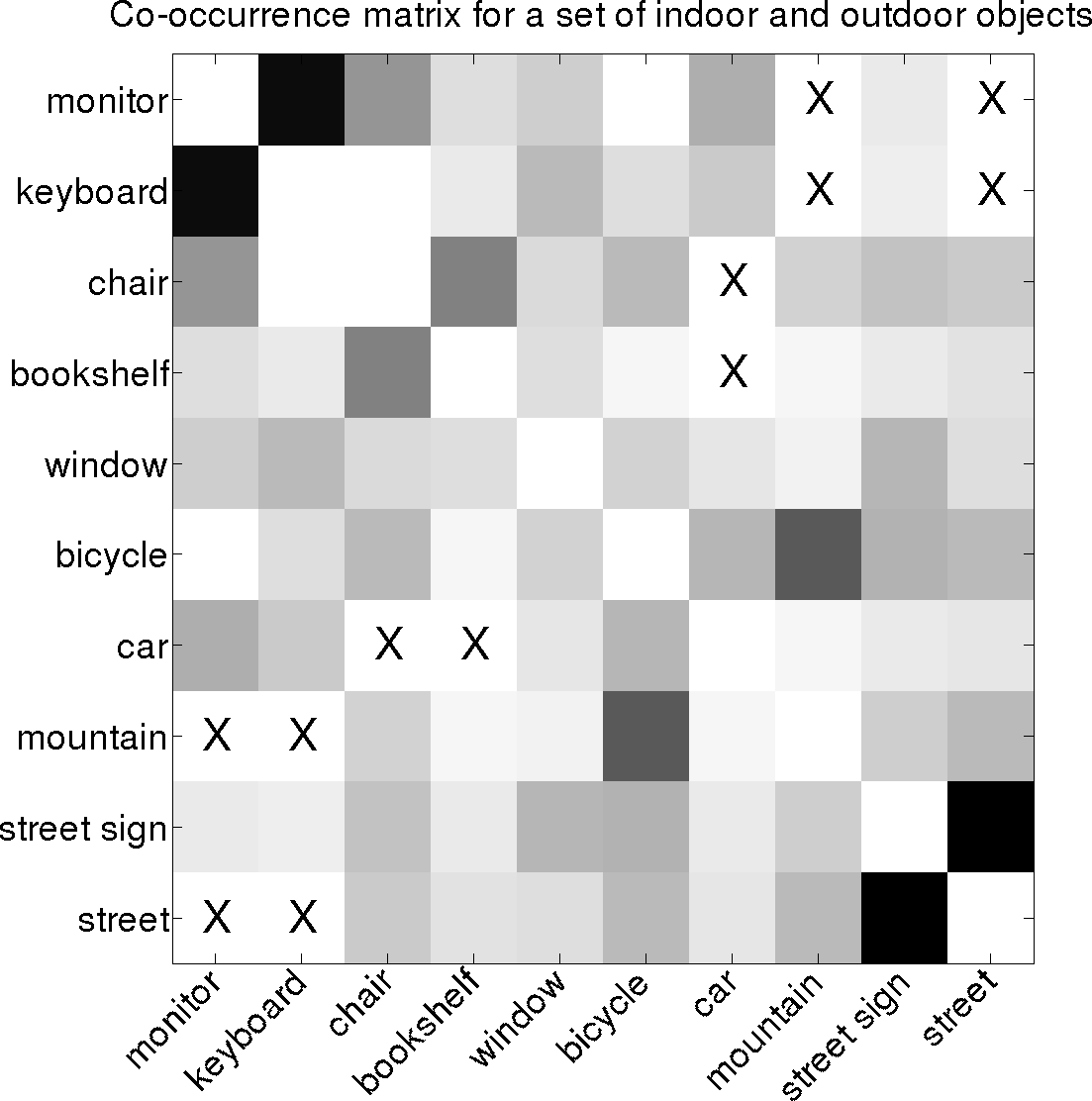
Figure 2: Graphical illustration of the co-occurrence scores for 10 object classes. Darker values show high correlation; crosses mean negative correlation; the diagonal is not used.

4 Experiments

In this section we report the results of two sets of experiments with public datasets. The first dataset, Sun12, is small yet the largest of its kind as each image is annotated with multiple labels. The second dataset, ImageNet for detection, is much larger but most images are associated with a single label.

In order to evaluate Laconic, we used the following metrics:

• Precision@$k$ is the number of correct labels returned in the top $k$ positions, divided by $k$.

• AveragePrecision is the mean of Precision@$k_{i}$ where $k_{i}$ is the position obtained by target label $i$, for all target labels.

• Detection@$k$ is the number of correct detections returned in the top $k$ positions, where a detection is valid if both the label is correct and the returned bounding box overlaps at least 50% with the target bounding box.

For each dataset, the training set was used to train a deep neural network (DNN) for classification. The validation set was used to select all hyper-parameters for the DNN and Laconic. The results for all the three metrics above are reported for the test sets.

4.1 Sun12

Sun12 is a subset of the SUN dataset [13], consisting of fully annotated images from SUN. To our knowledge, Sun12 is the largest publicly available dataset with multiple objects per image that spans thousands of classes. There is a total of 16,856 images containing 165,271 objects from 3,765 classes. We split the dataset in our experiments into disjoint sets of 85%, 10%, and 5% for training, validation and testing respectively. The training set contains about 10 examples per object. The test set consists of 798 images and is comprised of 7,761 annotated objects.

We created two types of co-occurrence matrices: one from web pages and one from the Sun12 training set. Since Sun12 contains multiple labels per image, we built a co-occurrence matrix of object classes that appear together in images from the training set. We report Laconic results using the web-induced co-occurrence matrix, a matrix constructed from the Sun12 training set, and a convex combination of both. The mixture coefficient was selected using the validation set.

For training the DNN we sampled around 1.5M cropped windows of varying sizes from the training set, each of which contains at least 70% of one target object. These were then used to train a large scale convolutional network similar to [8], which won the last ImageNet challenge. Concretely, the model consisted of several layers, each of which performed a set of convolutions followed by local contrast normalization and max-pooling. These layers were followed by several fully connected linear and sigmoidal layers, finally ending with a softmax layer with 3765 outputs, where each output corresponds to one of the object classes in Sun12. The full model was trained using stochastic gradient descent combined with the AdaGrad algorithm [3] along with the Dropout [6] regularization technique. We used mini-batches of size 128 and an initial learning rate of 0.001.

At test time, we extracted the following seven patches at inference time from the test image. The first is the largest possible square patch centered at the middle of the image, which we refer to as “the original crop box”. The rest of the patches were the original crop box enlarged by 5%, the original crop box shrunk by 5%, and the original crop box translated up, down, left and right by 5%. The prediction scores of these 7 boxes were then averaged.

We first ran a set of experiments in order to compare the various Laconic settings. Table 1 compares several combinations of the Laconic objective function described in (1), by varying the conformity term described in (2) and (3), or the co-occurrence term using either (4) or (6). We also tested the incorporation of domain constraints as described by (7). The combination consisting of a linear conformity term within the Ising model, a $2$-norm regularization without further domain constraints seems to yield good performance overall. These experiments used the co-occurrence matrix constructed from web pages. Furthermore, since the Ising model for general matrices is non-definite, we used 10 random initializations for $\boldsymbol{\alpha}$ and selected the best solution according to (1). Each inference of a single image took a few milliseconds on a standard Linux machine. In comparison, naively using a conditional random field such as the one described in [11], would require the evaluation of about ${3765\choose 5}$ combinations, which is greater than $10^{15}$. Instead, only a few thousands evaluations were required when using Laconic.

Table 1: Performance Results on the Sun12 Dataset for various losses.

Model vs Metric (%)	Precision@1	Precision@5	AveragePrecision
eqs (2) and (4)	86.2	53.1	76.3
eqs (3) and (4)	86.3	52.8	76.2
eqs (2), (4) and (7)	86.4	52.8	76.2
eqs (3), (4) and (7)	85.8	52.6	75.9
eqs (2), (6) and (7)	85.8	50.1	74.9

Table 2 provides comparison results of the baseline model (using the DNN only) to the various Laconic settings. In these experiments we evaluated three settings for the co-occurrence matrix: estimation using web data only, estimation using the Sun12 training set only, and a convex combination of both matrices, termed Mixture-Laconic in the table. As can be seen, the Laconic approach with the web co-occurrence matrix gives significantly better performance than both the baseline model and the Laconic approach with the Sun12 co-occurrence matrix. The combination of both co-occurrence matrices gives slightly better results overall.

Examples of classification results by the baseline and Laconic are shown in Figure 3, where we see that Laconic often surfaced labels that were not found by the baseline, based on the additional co-occurrence information. Figure 4 also compares Laconic to the baseline for precision@$k$ for various values of $k$. Again, it shows that Laconic’s performance is better than the baseline for all values of $k$.

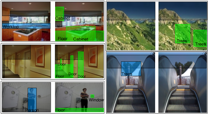
Figure 3: Example classifications by the baseline system and Laconic with localizations. In each example pair, the baseline classifications are on the left, and Laconic is on the right. Blue boxes with dark borders designate objects found only by the baseline. Green boxes with light borders designate objects found solely by Laconic. Black boxes designate objects found by both model.

Table 2: Performance results on the Sun12 Dataset for different co-occurrence sources.

Model vs Metric (%)	Precision@1	Precision@5	AveragePrecision
Baseline	85.7	50.6	75.0
Web-Laconic	86.2	53.1	76.3
Train-Laconic	85.5	50.8	75.1
Mixture-Laconic	86.1	53.7	76.6

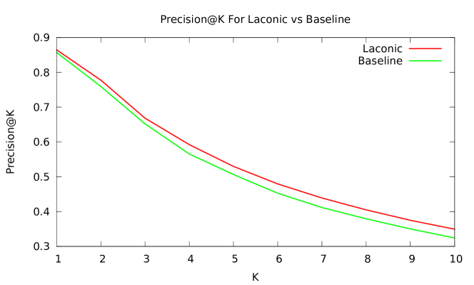
Figure 4: Precision@K comparing Laconic to baseline on the Sun12 dataset.

4.2 ImageNet Detection Dataset

Our second set of experiments is with the ImageNet dataset [2] (fall 2011 release). The entire dataset, typically used as a recognition benchmark, has almost 22,000 categories and 15 million images. A subset of this dataset is provided with bounding boxes which can be used for detection. There are 3623 categories that have bounding boxes and the total number of bounding boxes is 615,513. We divided the dataset into two subsets of equal size: half for training and half for testing.

We trained a deep neural network on this dataset. The architecture of the model is based on the model described in [9]. It consists of nine layers, has local receptive fields, employs pooling, local contrast normalization, and a softmax output layer for multiclass prediction.

To safeguard from overfitting, we added translated versions of the bounding boxes and negative examples. First, for every instance of the bounding boxes, we cropped 10 images, each translated up to 15 pixels in the horizontal and vertical directions. These transformations yielded about three million positive instances. Next, we sampled negative patches and treated them as a “background” category. To this end, we sampled random patches from the training images and made sure that the overlapping area with the correct bounding boxes is less than 30% of the total area. We also sampled examples that are difficult to classify by extracting patches that overlap with the correct bounding boxes at the four corners. The total number of negative (background) images is twelve million. Each of the above image patches were resized to an image consisting of 100x100 pixels. The total number of training images that were provide to learning algorithm for the deep neural network was fifteen million.

Training was performed using stochastic gradient descent with mini-batches. The resulting deep neural network was used for detecting objects in the training set using a sliding window. The sliding window procedure was applied at nine different scales where the $i$’th replica was of size $1.1^{i}$ of the base window size. For a specific scale, the overlap between one window to the next window is 80% of the size of the window. The windows were then resized to images of 100x100 pixels each using cubic interpolation. The patches were then fed to the deep network to obtain predictions. The above scheme is naturally massively parallelized in the inference step.

In order to asses the improvement of Laconic over the deep neural network we performed evaluation of two tasks: detection and classification. Since the co-occurrence matrix is extracted from the web pages, it may not convey any location information, and thus cannot help in localizing objects. It is therefore an interesting experiment on its own to see whether the external text-based information can improve the detection accuracy. Table 3 compares the performance of the baseline network with Laconic for two values of $k$: $k=1$ and $k=5$. The results show that Laconic substantially improves both classification and detection.

Metric (%)	Baseline	Web-Laconic
Precision@1	24.8	34.8
Precision@5	8.9	10.9
AveragePrecision	41.7	50.2
Detection@1	13.7	19.8
Detection@5	25.8	29.1

Table 3: Performance results on ImageNet

Note that even when there only a single object class is associated with an image, Laconic can help in “surfacing” the correct class even if it is not the most likely class according to the baseline DNN output. Indeed, most images are typically under-labelled. That is, there are more objects that appear in the images and thus could have been added to the set of labels (object classes) of the image. Since ImageNet was manually labeled where most images were associated with a single label, the existence of additional objects that tend to co-occur in natural text can improve the classification accuracy. In other words, if the patch classifier assigned high values to related object classes albeit not the single target class, Laconic can increase the likelihood of the correct target class, leveraging the co-occurrence information between the target class and the aforementioned object classes.

Finally, it is worth noting that all results provided for the ImageNet detection dataset, showing that Laconic was better than baseline, are statistically significant with 99% confidence, given the size of the test set. On the other hand, the Sun12 dataset being so small, none of the results are statistically significant, even at the 90% level.

5 Conclusion

Image classification becomes a difficult task as the number of object classes increases. We proposed a new approach for incorporating side information extracted from web documents with the output of a deep neural network in order to improve classification and detection accuracy. We empirically evaluated our algorithm on two different datasets, Sun12 and Imagenet, and obtained consistent improvements in classification and detection accuracy on both datasets.

In future work we plan to go one step further and incorporate spatial textual information. For instance, we could count the number of times we observe sentences such “the chair is beside the table” or “the car is under the bridge” and construct triplets of the form $(object_{1},relation,object_{2})$, where the relation expresses a spatial correspondence between the two objects. Such information could potentially lead to a more comprehensive and accurate visual scene analysis.

On the inference front, we plan to investigate alternative tractable approaches. For instance, approaches based on belief propagation have been used for related machine vision tasks. However, our preliminary experiments with belief propagation yielded poor performance and are thus not reported in the paper.

References

- [1] N. Chen, Q.-Y. Zhou, and V. K. Prasanna. Understanding web images by object relation network. In Proceedings of the 21st World Wide Web Conference, pages 291–300, 2012.
- [2] J. Deng, W. Dong, R. Socher, L.-J. Li, K. Li, and L. Fei-Fei. Imagenet: A large-scale hierarchical image database. In IEEE Computer Vision and Pattern Recognition (CVPR), 2009.
- [3] J. C. Duchi, E. Hazan, and Y. Singer. Adaptive subgradient methods for online learning and stochastic optimization. Journal of Machine Learning Research, 12:2121–2159, 2011.
- [4] C. Galleguillos, A. Rabinovich, and S. Belongie. Object categorization using co-occurence, location and appearance. In IEEE Conference on Computer Vision and Pattern Recognition (CVPR), 2008.
- [5] G. Heitz and D. Koller. Learning spatial context: Using stuff to find things. In ECCV, pages 30–43. Springer, 2008.
- [6] G. E. Hinton, N. Srivastava, A. Krizhevsky, I. Sutskever, and R. R. Salakhutdinov. Improving neural networks by preventing co-adaptation of feature detectors. arXiv preprint arXiv:1207.0580, 2012.
- [7] E. Ising. Beitrag zur theorie des ferromagnetismus. Z. Phys., 31:253–258, 1925.
- [8] A. Krizhevsky, I. Sutskever, and G. E. Hinton. Imagenet classification with deep convolutional neural networks. In P. L. Bartlett, F. C. N. Pereira, C. J. C. Burges, L. Bottou, and K. Q. Weinberger, editors, NIPS, pages 1106–1114, 2012.
- [9] Q.V. Le, M.A. Ranzato, R. Monga, M. Devin, K. Chen, G.S. Corrado, J. Dean, and A.Y. Ng. Building high-level features using large scale unsupervised learning. In International Conference on Machine Learning, 2012.
- [10] L. Rabiner and B.-H. Juang. Fundamentals of Speech Recognition. Prentice Hall, 1993.
- [11] A. Rabinovich, A. Vedaldi, C. Galleguillos, E. Wiewiora, and S. Belongie. Objects in context. In International Conference on Computer Vision (ICCV), 2007.
- [12] A. Torralba. Contextual priming for object detection. International Journal of Computer Vision, 53(2):169–191, 2003.
- [13] J. Xiao, J. Hays, K. Ehinger, A. Oliva, and A. Torralba. Sun database: Large-scale scene recognition from abbey to zoo. In 2010 IEEE Conference on Computer Vision and Pattern Recognition (CVPR), pages 3485–3492, 2010.