Separate Constraints on Early and Late Cosmology
Abstract
Since the public release of Planck data, several attempts have been made to explain the observed small tensions with other datasets, most of them involving an extension of the CDM Model. We try here an alternative approach to the data analysis, based on separating the constraints coming from the different epochs in cosmology, in order to assess which part of the Standard Model generates the tension with the data. To this end, we perform a particular analysis of Planck data probing only the early cosmological evolution, until the time of photon decoupling. Then, we utilise this result to see if the CDM model can fit all observational constraints probing only the late cosmological background evolution, discarding any information concerning the late perturbation evolution. We find that all tensions between the datasets are removed, suggesting that our standard assumptions on the perturbed late-time history, as well as on reionisation, could sufficiently bias our parameter extraction and be the source of the alleged tensions.
1 Introduction
It is a well established fact that early cosmology history until photon recombination is well understood. What happens after this epoch relies however on a less solid ground. The nature of dark energy, the details of reionisation, the collapse of structures, all this rely on priors that are not well tested, or non-linear physics, and thus might bias our analysis.
As was done originally in Vonlanthen et al. (2010), it is possible to devise an analysis of the early cosmology parameters that is independent of assumptions concerning the late universe, providing so-called “agnostic” constraints, i.e. constraints without believing in any late-time cosmology model. In Audren et al. (2013), this analysis was done with the data sets available at the time, and improved in order to be also independent of the CMB lensing contamination. It provided a consistency check of our current standard model of early-cosmology.
The purpose of this paper is two-folds. In a first time to update this analysis to the current Planck data, while improving the method. Then, we propose to use this newly acquired knowledge about the early universe and treat it as a measurement of early quantities, in the sense that it gives posterior distribution on a set of cosmological parameters. From there, one can assume a model for the homogeneous late-time evolution, and test the implications of the previous measurement on this model, as well as the information coming from other probes. The goal would then be to exclusively test the merit of the cosmological constant as an explanation for the late time acceleration, without any contamination from other assumptions. This second point could be extended in the future to more general models for late cosmology, involving e.g. neutrino masses or dynamical dark energy.
The main idea behind this approach is to be able to separate the effects of different assumptions on parameter extraction. In order to say that the CDM model is in tension with current measurements, one must be sure that this tension is a failure of the model to describe the late-time acceleration, and is not due to some of our assumptions about structure formation, or about reionisation, for instance. We will therefore adopt a simple CDM model for the late homogeneous cosmology.
With the recent release of Planck temperature anisotropies map, it is possible to apply these ideas and see how it affects the analysis. Indeed, there are some tensions between the current Planck analysis Ade et al. (2013a); Ade et al. (2013b) and the results of other cosmological probes: as it has for instance been pointed out in Verde et al. (2013), current existing constraints on the value of disagree with each other. One example is the discrepancy between the Planck result: km s-1 Mpc-1, and the Hubble Space telescope measurement: km s-1 Mpc-1, at . Although only a tension, it might be a sign of something wrong in the theoretical assumptions. It has been proposed in Marra et al. (2013) that this tension could be partially lifted by taking into account the local gravitational potential at the position of the observer in the HST measurement, but this effect is not enough to sufficiently relieve the tension. Another mismatch exists between the value of as probed by the weak lensing of the CMB or through the Sunyaev-Zel’dovich cluster count identified with Planck - it may advocate for neutrino mass although this is not favored by Planck temperature anisotropies spectrum alone. A recent proposition states that these anomalies are alleviated when analysing in a different way the GHz map Spergel et al. (2013). We are assuming here that the standard, publicly available likelihood is correct.
The idea of the paper is to see if one can reduce the observed tensions, by assuming only a minimal number of hypotheses. It is interesting to check whether one can make all current experiments agree with each other, by performing first an “agnostic” early universe analysis, and then assuming CDM for the late-time homogeneous evolution. At the very least, it would show the importance of the missing assumptions, especially in the case of studying extended standard models.
In section 2, we will present an improved “agnostic” analysis method, and discuss its similarities and differences with the standard analyses. In section 3, we will show how to take one further step and derive constraints on a standard CDM model coming from different homogeneous probes. We will show and discuss the results in section 4 and conclude in section 5.
2 Agnostic Study
The main idea on which the so-called “agnostic” study Audren et al. (2013) relies on is the realisation that, at the level of the primary (unlensed) power spectrum, the late-time cosmological parameters of some standard scenarios have a clear effect. They simply globally rescale in amplitude (through in the Standard Model), or shift the position of the peaks through a rescaling of the multipoles (the action of a cosmological constant , for instance). Both effects behave as mentioned only for large multipoles (i.e. ). By allowing to marginalise over these parameters, one should in principle be able to extract constraints on early cosmology parameters, independent on our assumptions for the late evolution. This previous analysis however had arguably one weakness about the lensing treatment that we will address here, after recalling the basic principle of the method.
More mathematically, the effect of the late time parameters on the temperature anisotropies power spectrum is that of a global rescaling (), and an arbitrary scaling of the multipoles (). Given this freedom, one can super-impose exactly two power spectra coming from two universes with the same early composition, but different late time cosmological parameter (namely the reionisation depth and the Hubble parameter ). This is true as long as one removes from the data the information coming from the lowest multipoles, . In practice, when using WMAP data, we tested the dependence of the parameter estimation on the starting multipole of our analysis, and decided to use .
We do not have this freedom when using Planck likelihood, as the starting is fixed. We can, however, restrain from using the low multipole likelihood, and exploit only the likelihood for high multipole, starting at . In the future, we hope to be able to specify the starting of the analysis with the next releases of Planck likelihood codes.
As in this previous paper, if one would measure directly the primary anisotropies, the set of parameters probed by such an agnostic analysis would be the following:
| (1) |
Indeed, only the product and the angular diameter distance are constrained by the information contained in the CMB alone, when we allow for an arbitrary normalisation, and rescaling of multipoles.
Note that this discussion is still valid for other cosmological models where only the late evolution is different (e.g. with spatial curvature, non-zero neutrino mass, dynamical Dark Energy, but not for models with , varying constants, or Lorentz-violating dark energy).
Since one observes in reality lensed anisotropies, it is crucial to treat the effect of lensing on the CMB photons in the same agnostic way. In a normal analysis, the lensing potential is generated by the same initial power spectrum amplitude and tilt than the one generating the perturbations. However, this assumes that CDM is valid for the late-homogeneous evolution, and this assumption should not be used here.
If one wants to be as general as possible, this power spectrum can have any shape and amplitude, and should not be the same as the one generated by and . In Audren et al. (2013), two parameters and were introduced, for the lensing potential, that simply modified the shape of the original spectrum. Hence, and correspond to the standard amount of lensing generated by the underlying power spectrum in a CDM universe. In this parametrisation, the meaning of these value changes from one point in parameter space to the other, because they are defined with respect to the initial power spectrum.
Instead, in this paper, we reformulate the approach, and we use these two parameters and to define, on their own, respectively the amplitude and the tilt of the lensing potential, and allow to marginalise over them. In this way, if they are equal to and , respectively, it will mean that the lensing is caused by a late-time CDM universe. By allowing them to vary freely, we do not impose this prior knowledge. We moreover set the pivot scale of this lensing potential to coincide with the maximum of the lensing potential, which is roughly 1/Mpc for Planck data.
Finally, we set the effective number of relativistic species to , and we take one massive neutrino of a total mass of eV, as specified in the base analysis of the Planck study. These values impact the prediction of by km s-1 Mpc-1 - a significant change considering Planck error bars on the Hubble rate.
We run the Markov Chain Monte Carlo code Monte Python on Planck data, in which we only take the high- likelihood (starting at ). We discard the information coming from the WMAP polarisation data, and from the low- likelihood. We also discard the lensing reconstruction likelihood to avoid making hypotheses on structure formation.
The set of varied parameters is
It has to be noted that a similar approach was performed in the standard analysis Ade et al. (2013a), with only the lensing amplitude being varied (parameter in this paper), and not the lensing tilt. This was simply done to highlight the fact that the CMB alone preferred a value slightly higher than for this parameter. The test was done both with defined with respect to the initial power spectrum, and with defined on its own111http://www.sciops.esa.int/wikiSI/planckpla/index.php?title=File:Grid_limit68.pdf&instance=Planck_Public_PLA. These results were however not further investigated, especially the latter.
3 Constraining the late time homogeneous evolution
We have seen in the previous section how to obtain in principle a constraint on early cosmological parameters, with their posterior distribution and correlations, in a model-independent way. We want now to push the analysis further, and utilise this knowledge to determine whether or not CDM is a good model to explain the homogeneous evolution of the late-time universe.
The idea is to choose a model for the late-time evolution, namely the cosmological constant, and test its merit to explain the accelerated expansion. By basing our analysis on the “agnostic” study, we have indeed the possibility to test this single assumption, without involving any other one. This approach thus differs from the standard one by the fact that we test separately the hypotheses of the standard model, instead of evaluating the general merit of all of them considered at the same time.
To this end, we will restrict ourselves to a flat universe, and assume further that is fixed to its best-fit value from the “agnostic” study. Indeed, its mean value and its error bar are respectively five and ten times lower than the ones of . Additionally, as will not play any role in the homogeneous late-time evolution, it will be considered fixed in this study.
All this results in having the following set of varying parameters
| (2) |
From these two parameters, and the constant value of , we can deduce the value of . We then test this cosmological set of parameters against the following existing data on homogeneous cosmology:
-
1.
Direct Measurement: In Riess et al. (2011), the authors provide an updated measurement of the local value of coming from direct distance measurements. It is a simple Gaussian distribution centered on km s-1 Mpc-1, and a standard deviation of km s-1 Mpc-1.
-
2.
Supernovae: Type-IA supernovae act as standard candles - the luminosity produced by their explosion is thought to be a constant, regardless of their setup before the explosion. The experiment measures then the apparent luminosity of the supernovae, as well as its spectroscopic redshift. One can then ask the angular diameter distance from the cosmological code, compute the luminosity distance with the relation , and compare it with the observed one. Recalling that
(3) one would expect this probe to be sensitive both to the values of and . However, the likelihood formula uses a simple formula for each data point, with non zero correlations between them, as well as a marginalized nuisance parameter accounting for the absolute magnitude of the measurement. This leads that only the information on is extracted from this experiment. We used the data from Amanullah et al. (2010) (Union2 data) in this study.
-
3.
BAO: The observed Baryonic Acoustic Oscillation scale at a given redshift is given by the following ratio:
(4) where is the baryon drag scale (Photon and baryon are usually considered to decouple at the same time, but since there are much less baryons, they actually decouple slightly later than the photons (around ). This period where they are still in equilibrium with the remaining photons is called the drag epoch, and the drag scale thus marks the end of this epoch). The baryon drag scale is determined by the agnostic analysis, with an accuracy better than .
and are respectively the angular diameter and radial distances, measured at the redshfit of each galaxy. The denominator consists of the geometric mean of these two quantities, that both vary strongly with and . The BAO likelihood is then simply build as a formula on every measured point. The data used comes from 6dFGRS Beutler et al. (2011), SDSS-II Padmanabhan et al. (2012) (Data Release 7),and BOSS Anderson et al. (2013) (Data Release DR9).
The standard analysis of the BAO data relies on computing the baryon drag scale, as well as angular and radial distances at a given redshift, for each point in the parameter space during the parameter extraction. We adapted this method to consider the baryon drag scale as a measured quantity, coming from the agnostic study, with a best-fit and an error. We add both the measurement error from the BAO data and this measurement error from the agnostic study in quadrature, and keep the simple formula. It has to be noted that the baryon drag scale is measured with a precision of , so the error is dominated by the BAO error.
-
4.
Time Delay: Quasar Time-Delay measurements probe cosmological parameters through the time delay between different images of gravitationally strongly lensed quasars. The chosen quasars have a highly intrinsic variable light curve, which is then observed coming from separate positions, and thus having travelled through different path. The time-delay between the different images accounts for differences in the path, but also from the different Shapiro delays induced by the lensing galaxy (for an in-depth explanation of the measurement, see Tewes et al. (2012)). This time-delay distance is defined as follows:
(5) where is the angular diameter distance to the lens, the redshift of the lens, the angular diameter distance to the source and the angular diameter distance between source and lens. The data we used for this study is taken from Suyu et al. (2010) and Suyu et al. (2013), with a shifted log normal distribution.
Finally, we have to take into account the information coming from the early parameter analysis. To do this, we can realise that this first analysis gives the posterior distribution for , and . As seen previously, is a function of , and , for a flat universe. As mentioned previously, since is measured to a much greater precision than , and since only the sum of the two is involved in the late-time evolution, we fixed to its best-fit value.
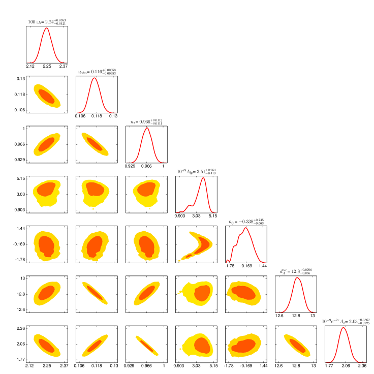
We thus use the 2-dimensional posterior distribution of and found with an “agnostic” analysis to define a multi-Gaussian likelihood, which seems a reasonable choice considering Fig 1. As these two parameters are found to be correlated in this first study, it is crucial that our likelihood takes into account this degeneracy. If one did not take into account this correlation, one would have lost a factor of two in the marginalised error bars. In the next section, this last experiment will be referred to as this work. It corresponds then to the constraint coming from Planck data alone, which will be compared with the aforementioned probes of homogeneous cosmology.
4 Results
4.1 “Agnostic” early universe results
After running MCMC chains with monte python222http://montepython.net, with a modified Metropolis-Hastings algorithm Lewis (2013), we obtain the best-fit, mean and one-sigma constraints for our “agnostic” parameters, as shown in table 1. In this table, we compare with the standard results based on the high-, low- Planck likelihoods as well as the WMAP polarisation. As we can see there, there are only minor shifts in central values for most of the parameters. The degradation of the error bar is not so significant.
Note that it was not possible to perform a comparison of the posterior distribution of the cosmological parameters between the agnostic approach and a standard analysis using only the high- likelihood. Indeed, this data set alone leaves unconstrained a degeneracy between and , leading to extremely poor convergence. It is only with the inclusion of the low- likelihood and the WMAP polarisation that converge is reached.
|l|c|c||c|ccccccc|
Parameters & This work Planck Standard
/
/
/
/
4.2 Late time universe results
The most important differences with respect to the standard analysis start to appear when analysing the late-time universe with minimal assumptions.
The mean values for the parameter, for all the different experiments, are summarised in table 2. One can notice on the first hand that, in addition to a wider error bar on the Hubble parameter, the central value being significantly different than the one from the published Planck analysis. The central value and marginalised posterior distribution at 1 are km s-1 Mpc-1, to contrast with km s-1 Mpc-1. Note first that the two values are in agreement at the level of 1, and that the discrepancy in both central value and marginalised width can be attributed to i) the contaminating effect coming from all the underlying assumptions usually done when considering the standard CDM universe - mainly reionisation and the growth of structures affecting the CMB lensing, and ii) the information coming from discarded region in multipole space.
| Direct Measurement | Supernovae | Time Delay | BAO | This Study | |
|---|---|---|---|---|---|
The two dimensional posterior distribution, showing the correlation between and contains more information, as seen in figs 2 and 3.
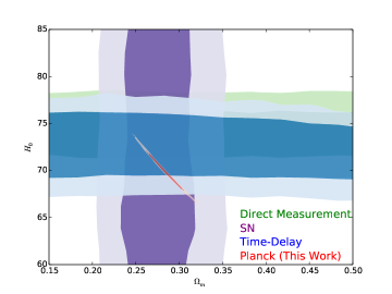
What we can already notice on fig 2 that the analysis presented in this study (red contours) agree well with the constraints coming from direct measurement, supernovae, and time-delay of quasars. By zooming in, one can see on fig 3 the particular region of interest. We left out the supernovae and time-delay constraints out for clarity, but added the BAO one, and the standard Planck analysis (blue contours).
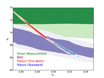
We can notice there the agreement between Planck standard result and this work, which has simply a much broader distribution along the degeneracy between the two parameters. Our more conservative analysis impacted the sensitivity to the cosmological parameters, thus reconciling Planck data with the direct measurement of , while maintaining the agreement with the BAO scale measurement.
One can also notice that any tension between the datasets has been lifted in this proposed analysis. Our claim is that our assumptions on the perturbed late-time universe, as well as on reionisation, are able to bias our prediction and could be the source of this observed tension.
5 Conclusion
We devised a way to test the merit of the cosmological constant as the source of our late time evolution, independently of structure formation. To this end, we performed a model-independent analysis of the early universe data coming from the Planck temperature anisotropies measurement, to obtain so called “agnostic” constraints on the early parameters. We then utilised this knowledge to constrain the parameter space of , and compared this analysis with other experimental probes of the homogeneous late-time universe.
We showed that, in contrast with the standard analysis, this study reconciles the local measurement of and Planck data, without sacrificing the agreement with the other datasets.
Our analysis demonstrated that some of the less often tested assumptions behind the Standard Model of Cosmology, like the reionisation history and the growth of structures, can play an important role in the determination of the posterior distribution of its parameters. It seems striking that the effects described here are on par with existing propositions for evidence for new physics in Planck data.
It is at the best of our knowledge not possible to further refine and pinpoint which assumption in particular is biasing the most the standard analysis in the direction of lower values. Indeed, to achieve this goal, one would need to compare this “agnostic” analysis of the high- likelihood with a standard analysis of the same. However, as discussed above, the presence of a large degeneracy between and prevents the convergence of the parameter extraction in this case.
It is not our point to pretend that this method is a better way to reconcile the datasets than any other proposition, but rather to highlight the importance of testing as thoroughly as possible every underlying assumptions of our standard model of cosmology.
This only further highlights the fact that the Planck satellite opened the doors of a precision era in our field. Such effects were previously considered unimportant, because of the lack of resolution of past experiments. With access to such a high sensitivity experiment, a better understanding of the underlying assumptions behind our Standard Model, notably the role of reionisation and structure formation, seems to be in order.
Acknowledgments
We would like to thank Julien Lesgourgues for crucial comments and suggestions about the analysis and the draft, as well as Antony Lewis for his pertinent remark on the lensing potential amplitude. This project is supported by a research grant from the Swiss National Science Foundation.
References
- Ade et al. (2013a) Ade P., et al., 2013a
- Ade et al. (2013b) Ade P., et al., 2013b
- Amanullah et al. (2010) Amanullah R., Lidman C., Rubin D., Aldering G., Astier P., et al., 2010, Astrophys.J., 716, 712
- Anderson et al. (2013) Anderson L., Aubourg E., Bailey S., Bizyaev D., Blanton M., et al., 2013, Mon.Not.Roy.Astron.Soc., 427, 3435
- Audren et al. (2013) Audren B., Lesgourgues J., Benabed K., Prunet S., 2013, JCAP, 1302, 001
- Beutler et al. (2011) Beutler F., Blake C., Colless M., Jones D. H., Staveley-Smith L., et al., 2011, Mon.Not.Roy.Astron.Soc., 416, 3017
- Lewis (2013) Lewis A., 2013, Phys.Rev., D87, 103529
- Marra et al. (2013) Marra V., Amendola L., Sawicki I., Valkenburg W., 2013, Phys. Rev. Lett. 110,, 241305
- Padmanabhan et al. (2012) Padmanabhan N., Xu X., Eisenstein D. J., Scalzo R., Cuesta A. J., et al., 2012, Mon.Not.Roy.Astron.Soc., 427, 2132
- Riess et al. (2011) Riess A. G., Macri L., Casertano S., Lampeitl H., Ferguson H. C., et al., 2011, Astrophys.J., 730, 119
- Spergel et al. (2013) Spergel D., Flauger R., Hlozek R., 2013
- Suyu et al. (2013) Suyu S., Auger M., Hilbert S., Marshall P., Tewes M., et al., 2013, Astrophys.J., 766, 70
- Suyu et al. (2010) Suyu S., Marshall P., Auger M., Hilbert S., Blandford R., et al., 2010, Astrophys.J., 711, 201
- Tewes et al. (2012) Tewes M., Courbin F., Meylan G., 2012
- Verde et al. (2013) Verde L., Protopapas P., Jimenez R., 2013
- Vonlanthen et al. (2010) Vonlanthen M., Rasanen S., Durrer R., 2010, JCAP, 1008, 023