Planetary Candidates Observed by Kepler IV: Planet Sample From Q1-Q8 (22 Months)

Christopher J. Burke¹, Stephen T. Bryson², F. Mullally¹, Jason F. Rowe¹, Jessie L. Christiansen³, Susan E. Thompson¹, Jeffrey L. Coughlin¹, Michael R. Haas², Natalie M. Batalha², Douglas A. Caldwell¹, Jon M. Jenkins¹, Martin Still⁴, Thomas Barclay⁴, William J. Borucki², William J. Chaplin⁵^,6, David R. Ciardi³, Bruce D. Clarke⁷, William D. Cochran⁸, Brice-Olivier Demory⁹, Gilbert A. Esquerdo¹⁰, Thomas N. Gautier III⁷, Ronald L. Gilliland¹¹, Forrest R. Girouard¹², Mathieu Havel², Christopher E. Henze², Steve B. Howell², Daniel Huber², David W. Latham¹⁰, Jie Li¹, Robert C. Morehead¹³^,21, Timothy D. Morton¹⁴, Joshua Pepper¹⁵^,16, Elisa Quintana¹, Darin Ragozzine¹⁷, Shawn E. Seader¹, Yash Shah¹⁸, Avi Shporer¹⁹, Peter Tenenbaum¹, Joseph D. Twicken¹, Angie Wolfgang²⁰^,21 ¹SETI Institute/NASA Ames Research Center, Moffett Field, CA 94035 ²NASA Ames Research Center, Moffett Field, CA 94035 ³NASA Exoplanet Science Institute/Caltech, Pasadena, CA 91125 ⁴Bay Area Environmental Research Institute/NASA Ames Research Center, Moffett Field, CA 94035 ⁵School of Physics and Astronomy, University of Birmingham, Edgbaston, Birmingham, B15 2TT, UK ⁶Stellar Astrophysics Centre (SAC), Department of Physics and Astronomy, Aarhus University, Ny Munkegade 120, DK-8000 Aarhus C, Denmark ⁷Jet Propulsion Laboratory/California Institute of Technology, Pasadena, CA 91109 ⁸Astronomy Department and McDonald Observatory, The University of Texas, Austin TX 78712 ⁹Department of Earth, Atmospheric and Planetary Sciences, Massachusetts Institute of Technology, 77 Massachusetts Ave., Cambridge, MA 02139 ¹⁰Harvard-Smithsonian Center for Astrophysics, 60 Garden Street, Cambridge, MA 02138 ¹¹Center for Exoplanets and Habitable Worlds, The Pennsylvania State University, University Park, PA 16802 ¹²Orbital Sciences Corporation/NASA Ames Research Center, Moffett Field, CA 94035 ¹³Department of Astronomy and Astrophysics, The Pennsylvania State University, University Park, PA 16802 ¹⁴Department of Astrophysics, California Institute of Technology, MC 249-17, Pasadena, CA 91125 ¹⁵Department of Physics, Lehigh University, 16 Memorial Drive East, Bethlehem, PA 18015 ¹⁶Department of Physics and Astronomy, Vanderbilt University, 6301 Stevenson Center, Nashville, TN 37235 ¹⁷Department of Physics and Space Sciences, Florida Institute of Technology, 150 West University Blvd., Melbourne, FL 32901 ¹⁸University of California, Berkeley, Berkeley, CA 94720 ¹⁹Division of Geological and Planetary Sciences, California Institute of Technology, Pasadena, CA 91125 ²⁰Department of Astronomy and Astrophysics, University of California, Santa Cruz, CA 95064 ²¹NSF Graduate Research Fellow christopher.j.burke@nasa.gov

Abstract

We provide updates to the Kepler planet candidate sample based upon nearly two years of high-precision photometry (i.e., Q1-Q8). From an initial list of nearly 13,400 Threshold Crossing Events (TCEs), 480 new host stars are identified from their flux time series as consistent with hosting transiting planets. Potential transit signals are subjected to further analysis using the pixel-level data, which allows background eclipsing binaries to be identified through small image position shifts during transit. We also re-evaluate Kepler Objects of Interest (KOI) 1-1609, which were identified early in the mission, using substantially more data to test for background false positives and to find additional multiple systems. Combining the new and previous KOI samples, we provide updated parameters for 2,738 Kepler planet candidates distributed across 2,017 host stars. From the combined Kepler planet candidates, 472 are new from the Q1-Q8 data examined in this study. The new Kepler planet candidates represent $\sim$ 40% of the sample with ${\rm R_{P}}$ $\sim$ 1 ${\rm R_{\oplus}}$ and represent $\sim$ 40% of the low equilibrium temperature ( ${\rm T_{eq}}$ $<$ 300 K) sample. We review the known biases in the current sample of Kepler planet candidates relevant to evaluating planet population statistics with the current Kepler planet candidate sample.

Subject headings:

catalogs – eclipses – planetary systems – space vehicles

I. Introduction

The NASA Kepler spacecraft delivers high precision photometric observations to identify large samples of transiting planets around stars in the Milky Way Galaxy. One of its primary science drivers is to extend our knowledge of extrasolar planets to the regime of Earth-size planets orbiting stars like the Sun (Borucki et al., 2010). The Kepler project has released a series of papers incrementally increasing the planet candidate discoveries identified with Kepler data (Borucki et al., 2011a, b; Batalha et al., 2013). This study is the continuation of this series applied to transiting planet signals detected in 8 quarters, Q1-Q8, (nearly two years) worth of Kepler data. In addition to the new planet candidates, we re-evaluate the Kepler planet candidates from Borucki et al. (2011a, b) that were announced using the earliest available Kepler data. Re-evaluating the earliest Kepler planet candidates increases the baseline of observations and takes advantage of the more refined techniques for evaluating the reliability and source of the transit signal.

The Kepler planet candidate sample is the basis for a wide variety of exoplanetary studies and discoveries. A subset of the Kepler planet candidate sample has been confirmed using radial velocity follow up (e.g., Dunham et al., 2010; Latham et al., 2010; Batalha et al., 2011; Endl et al., 2011; Santerne et al., 2011; Hébrard et al., 2013), statistical analysis of the Kepler flux time series in order to rule out stellar binary signals (e.g., Torres et al., 2011; Morton & Johnson, 2011; Fressin et al., 2011; Borucki et al., 2012; Wang et al., 2013; Barclay et al., 2013), and transit time variations (e.g., Holman et al., 2010; Lissauer et al., 2011a; Fabrycky et al., 2012a; Ford et al., 2012; Steffen et al., 2012; Xie, 2013). Studying the population of multiple planet candidate systems provides insight into the formation, migration, and dynamical interaction processes that result in the planets observed by Kepler (e.g., Ford et al., 2011; Lissauer et al., 2011b; Fabrycky et al., 2012b; Rein, 2012; Hansen & Murray, 2013; Batygin & Morbidelli, 2013). The underlying planet population in the Galaxy can be determined from the observed planet candidate sample from Kepler using a thorough understanding of the selection effects and sources of contamination (e.g., Youdin, 2011; Howard et al., 2012; Fressin et al., 2013; Christiansen et al., 2013; Dressing & Charbonneau, 2013).

In § II the Kepler data analysis pipeline is reviewed and the process used to select the transit signals for analysis is described. § III & § IV detail the analysis techniques employed using Kepler data alone to ensure a high degree of probability that the transit signal originates from the target star under observation and eliminate possible sources of false positives. The purpose of this analysis is to classify the transit signals as either a planet candidate or false positive. The transit signals are fit to a planet model, § V, to determine planet parameters after assigning stellar parameters following the procedure outlined in Batalha et al. (2013). We describe the resulting population of planet candidates discovered by Kepler in § VI, and we conclude the study in § VII.

II. Transit Signal Detection

Identification of planet candidates in Kepler data begins with output from the Kepler science pipeline. The Kepler pipeline converts the raw instrument output of the Kepler spacecraft into a format usable by the scientific community (see Jenkins et al., 2010, for an overview). Here we summarize only the Transiting Planet Search (TPS) module of the Kepler pipeline as it performs the transit signal detection using output of the earlier modules of the Kepler pipeline that provide instrument corrected aperture flux time series data. TPS empirically determines the noise in the flux time series (combined differential photometric precision, CDPP, Christiansen et al., 2012) of each target to search for potential planet candidates (threshold crossing events, TCEs) (Jenkins, 2002; Tenenbaum et al., 2012). For a transit signal in Kepler data to be defined as a TCE, the combined signal-to-noise ratio (SNR) from multiple transit events (the multiple event significance, MES) must be above a preset threshold, MES $>$ 7.1 (Jenkins, 2002). In addition, a transit signal must have a ratio of the MES to the strongest single transit event SNR greater than $\sqrt{2}$ in order to qualify as a TCE (Tenenbaum et al., 2012). The criteria for identifying a TCE has evolved through time, and the specifics described above pertain to what was used in the Q1-Q8 Kepler pipeline run. The input light curve input to TPS for the Q1-Q8 pipeline run was generated by the Pre-search Data Conditioning (PDC) algorithm as described by Twicken et al. (2010a).

In its simplest form a TCE represents a transit candidate by specifying the target Kepler Input Catalog (KIC) identifier (Brown et al., 2011), ephemeris period, ephemeris epoch, transit duration estimate, and transit depth estimate. In November 2011, the Q1-Q8 (22 months of data) pipeline run generated one or more TCEs for $\sim$ 13,400 Kepler targets out of $\sim$ 191,000 targets searched.

III. TCE Triage

The majority of TCEs ( $\gtrsim$ 80%) are not valid planet candidates. Contributing are numerous types of astrophysical variability: stellar oscillations (Aerts et al., 2010), overcontact binaries (Sirko & Paczyński, 2003), tidal dynamic distortions (Thompson et al., 2012), and broad-band “red noise”. In addition, the TCE population is contaminated by signals due to instrumental effects: thermal transients, pixel sensitivity dropouts, pattern noise, and video crosstalk (Caldwell et al., 2010; Kolodziejczak et al., 2010; Stumpe et al., 2012). Most of these contaminants do not produce the archetypical signal for a transiting planet, characterized by repetitive, isolated, limb-darkened events with out-of-transit noise that averages down as expected for independent data.

In order to efficiently remove the contaminating signals in the TCE sample, all TCEs undergo a visual inspection of the Kepler light curve data phase folded on the TCE ephemeris. A standardized data plot is generated for the TCE found for a given target in TPS. The data plot employs the aperture flux time series generated by the Photometric Analysis (PA) module of the pipeline (Twicken et al., 2010b). For plotting, the flux time series is median detrended with a moving window of 2 day duration and the resulting relative flux time series is phase folded on the TCE ephemeris. We perform this “triage” stage for the $\sim$ 13,400 TCEs, using the phase folded relative flux time series. The TCE is either accepted as a potential planet candidate from visual inspection of the phase folded flux time series and moves onto the next stage of vetting, or the TCE is eliminated from further consideration as a planet candidate.

During “triage”, 565 TCEs were identified around 480 new Kepler targets that did not have previously known transit signal detections. The TCEs that pass the visual inspection “triage” stage are designated as Kepler Objects of Interest (KOI). A TCE that passes “triage” is assigned a KOI number in order to catalog the detection and to move forward in its analysis as a potential planet candidate. The Q1-Q8 TCEs that passed “triage” were assigned KOI numbers in the range 2668 $\leq$ KOI $\leq$ 3149. It is important to emphasize that a KOI at this earliest stage has not been vetted against the full complement of Kepler data and analysis tests as described in § IV. The KOI sample before dispositioning still has a high proportion of false positives due to stellar binaries, instrumental artifacts, and other astrophysical variability. In subsequent dispositioning (described in § IV) $\sim$ 40% of the new KOIs were given a false positive designation.

IV. Kepler Object of Interest Dispositioning

For a newly created KOI to be dispositioned as a planet candidate it must pass further scrutiny using Kepler data. Primarily, the KOI dispositioning examines both the flux time series data, for consistency with the expectation of a transiting planet signal, and the pixel-level time series data, for consistency with the expectation that the signal originates from the target of interest in the aperture. The dispositioning process follows the general procedure outlined in Batalha et al. (2013). The present updates to the KOI sample result from dispositioning two groups of Kepler targets. The first group of targets are new KOIs that were identified in the Q1-Q8 data as outlined in § II & III. The new KOIs in this group are in the range 2668 $\leq$ KOI $\leq$ 3149. The second group of targets are the earliest KOIs (KOI number $\leq$ 1609) from the first two Kepler planet candidate catalogs (Borucki et al., 2011a, b). These KOIs are re-evaluated to take advantage of the substantially increased data baseline and a more uniform set of dispositioning criteria and procedures. Overall, between the two groups of KOIs, we evaluated $\sim$ 1900 KOIs around $\sim$ 1500 targets. The most current analysis of KOIs intermediate between these two groups, 1610 $\leq$ KOI $\leq$ 2667, is published in Batalha et al. (2013). The KOI sample of Batalha et al. (2013) also added new KOIs in the $\leq$ 1609 range that were discovered in multiplanet systems that we do not revisit in this study. As described in § VI, Table 1 contains a binary flag to indicate whether the KOI was vetted during this study.

Although the new KOIs reported here were discovered from the search of Q1-Q8 data, the actual data products used for dispositioning were from a Q1-Q10 (28 months) pipeline run. Results from the Q1-Q10 pipeline run were the most current pipeline products at the disposal of the authors at the outset of the dispositioning (May 2012). For the two groups of KOIs that are a part of this study, we also dispositioned any new TCEs that were discovered in the Q1-Q10 data and included them in this KOI sample. We did not evaluate new TCEs from the Q1-Q10 pipeline run for the intermediate, 1610 $\leq$ KOI $\leq$ 2667, targets or other Q1-Q10 targets that were not previously known to have KOIs. This inhomogeneity in the planet candidate sample has implications for statistical studies of the underlying planet population as discussed in § IV.4.

KOI dispositioning is primarily based upon a report and its separate summary that are generated in the Data Validation (DV) module of the pipeline (Wu et al., 2010). DV report summaries are available from the subsequent Q1-Q12 pipeline run hosted at the NASA Exoplanet Archive¹¹1http://exoplanetarchive.ipac.caltech.edu. The Q1-Q12 results are not available for all the KOIs examined in this study since the pipeline runs are independent and subsequent runs are not guaranteed to identify the same transiting signal. 95% of the cumulative Kepler planet candidate sample have Q1-Q12 DV products available at the NASA Exoplanet Archive.

The DV report summary provides the Kepler flux time series and pixel-level data tests that are most relevant for dispositioning the KOI into one of three categories: planet candidate, needs further scrutiny, or false positive. The criteria and statistical tests for dispositioning a KOI are outlined in Batalha et al. (2013) and are discussed further in § IV.1 and § IV.2. Every KOI had at least two individuals independently evaluate all criteria in order to judge its planet candidate status. KOIs with unanimous evaluation as a planet candidate or false positive are dispositioned as a planet candidate or false positive, respectively. KOIs with a discordant disposition are given additional scrutiny. After the first manual vetting process $\sim$ 35% of targets required additional scrutiny. Most targets can be decided upon with the DV data products, however some targets undergo scrutiny using additional data analysis tools when tests using the standard data products are inconclusive or unavailable.

IV.1. Flux Time Series Dispositioning

The precision of the flux time series is sufficient to distinguish some categories of stellar binaries that can mimic a transiting planet (Brown, 2003; Torres et al., 2004). In this section we describe three criteria evaluated to determine whether the observed flux time series for a KOI is consistent with a planet candidate or false positive. The first criterion investigates the presence of a “secondary” transit event in the flux time series data with the same period as the KOI. The presence of a secondary suggests the signal originates from two self-luminous bodies undergoing mutual eclipses and is a strong indicator of a stellar binary false positive. A phase-folded median-filtered (filter window is the geometric mean of the transit duration and orbital period) using an updated version of the PDC flux time series (Stumpe et al., 2012; Smith et al., 2012) is visually examined for evidence of a secondary. Often a significant secondary also triggers an additional TCE at the same period. If an apparent secondary event is present, the secondary is reexamined in both PA flux time series with a median detrended filter applied and a PDC flux time series with a wavelet whitening filter applied (as employed during the planet search in TPS, Jenkins, 2002). A consistent and visually significant secondary event in all filtering methods results in a false positive disposition. To prevent planetary candidates with secondary occultations from being dispositioned as false positives, the secondary event is fit for its depth to estimate the geometric albedo and its uncertainty following Rowe et al. (2006). An estimated geometric albedo ${\rm A_{g}}>$ 1.0 with 3 $\sigma$ confidence implies that a statistically significant amount of flux is being emitted by the planet beyond the expected amount due to reflection alone. KOIs with ${\rm A_{g}}<$ 1.0 maintain their planet candidate status even with the presence of a secondary since we cannot rule out a planet candidate that produces a secondary through reflected light or thermal emission.

The second criterion measures whether there is a statistically significant difference in the transit depth between alternating events. A statistically significant depth difference implies that the KOI is a stellar binary with an orbital period twice the KOI ephemeris period with similar primary and secondary depths (although different enough to statistically confirm the depth difference). The odd-even depth test implements independent transit model (Mandel & Agol, 2002) fits to the odd- and even-numbered transit events and measures the statistical difference in the resulting transit depths. The results of the transit model fits are available in the DV report summary. A KOI is designated a false positive if the odd-even depths are statistically different ( $>$ 3 $\sigma$ ) from the model fits and a visual examination of the phased odd-even light curves agrees with this assessment. The false positives identified by the odd-even depth test are confirmed with model fits independent of the pipeline analysis using an alternative filtering of the data that uses a median detrended PA flux time series.

The final criterion examined in the flux times series is a qualitative judgment as to the reliability and uniqueness of the transit signal. The reliability of the transit signal is visually judged based upon the several panels displaying the flux time series on the DV report summary. Having features of similar depth and duration in the phase folded out-of-transit baseline data results in designating the KOI as a false positive. The process for examining the transit signal reliability for KOIs is similar to the TCE triage steps (see § III). However, the dispositioning process is more thorough. During KOI dispositioning an object can be subjected to additional follow up analysis using data products beyond the DV report summary when necessary.

IV.2. Pixel-level Time Series Dispositioning

The second phase of dispositioning focuses on the pixel-level time series data (Batalha et al., 2013; Bryson et al., 2013) available at the Mikulski Archive for Space Telescopes (MAST)²²2http://archive.stsci.edu. The diagnostics based upon pixel-level data determine whether the transit-like signal originates from the target or is spatially offset. A transit signal that conclusively does not originate from the designated target in the photometric aperture is designated a false positive. If the pixel-level data are consistent with a transit on the target or the tests are inconclusive, then it is designated as a planet candidate. Bryson et al. (2013) describes the process for combining these diagnostics into a decision for dispositioning the pixel-level data. We briefly describe the pixel-level diagnostics here.

There are two pixel diagnostics employed to locate the origin of the transit signal. The first diagnostic is a stellar image position time series using a flux-weighted centroiding algorithm. A statistically significant offset in the flux-weighted centroid during transit indicates that the target star is not isolated but has contaminating flux in the aperture from other sources (Wielen, 1996). The detector row and column positions of the image are calculated using a flux-weighted centroid algorithm for every cadence and converted into a time series of RA and declination positions from a pixel to coordinate transformation determined in PA. The RA and declination position time series is median-filtered with a window of 48 Kepler long cadences ( $\sim$ 30 min in duration) and phase folded on the KOI ephemeris. In order to determine the change in image position during transit, the Mandel & Agol (2002) transit model using parameters from the fit to the flux time series is fit to the centroid time series. In this case, the only free parameter in the model is a scale factor that converts the fixed transit model into the relative change in the image position. The statistical significance of the centroid offset and its direction during transit is the diagnostic considered for dispositioning. Figures supporting the centroid time series fit are provided in the DV products for each TCE (see Figures 4 & 5 of Bryson et al., 2013, for a description of their use in dispositioning). Since it indicates whether the stellar flux observed in the aperture is composed of multiple sources, a significant change in the flux weighted centroid during transit does not by itself indicate that the source of the transit signal is not on the primary target of the photometric aperture. Thus, the flux weighted centroid information plays a supporting role to the second pixel-level diagnostic described next.

The second diagnostic considered from the pixel-level data is based on consideration of flux difference images. A flux difference image is calculated for every observing quarter that contains transit events by determining the average change in flux during transit based upon the ephemeris of the TCE. This is done on a pixel-by-pixel basis in order to spatially locate the source of the transit signal on the detector. A flux difference image is good quality and provides useful information when it has the appearance of a stellar point spread function (PSF) (see Figure 11 of Bryson et al., 2013, for examples of a high quality flux difference image). Stellar crowding, low SNR transit events, saturated stars, and various systematics can result in difference images that are qualitatively inconsistent with a stellar image and invalidate the results of the next pixel-level disposition criterion. In the test considered here, a visual inspection is performed in order to determine whether a majority of the flux difference images are consistent with a stellar PSF. In the case when a majority of the flux difference images are of poor quality, the KOI is given a planet candidate disposition since the pixel-level disposition criterion based upon the flux difference images will be unreliable.

If the transit signal originates from the target of interest in the photometric aperture, then the flux difference image will have the appearance of a stellar point spread function (PSF) centered on the target location. A flux difference image that has the appearance of a stellar PSF and has a statistically significant offset from the target is evidence for a false positive. To quantify the position of the flux difference image, the Kepler Pixel Response Function (PRF) model (described in Bryson et al., 2010, and available through MAST) is fit to the flux difference image. A $\chi^{2}$ minimization solves for the stellar position and brightness that minimizes the residual between the observed and model images. The out-of-transit position of the target is determined by two methods: 1) adopting the KIC position as the target position and 2) performing another PRF model fit to the “direct” image to determine the target position. The direct image is based upon averaging a contiguous, but limited, set of out-of-transit images that occur before and after all transit events in a quarter. The set of contiguous out-of-transit images has the same duration as the transit, but it is offset by 3 observing cadences preceding and following the first and fourth contact of the transit event, respectively.

The observed target position from the direct image is the preferred comparison to the flux difference image, however, the KIC position provides a more robust position when stellar crowding results in a biased direct image position. For each observing quarter an offset and its uncertainty are calculated between the flux difference image and both target position estimates. The single-quarter results are combined to derive a robust average offset across multiple quarters. An average position offset $>$ 3 $\sigma$ results in a false positive designation. In general, both the direct image position and KIC position offsets should be $>$ 3 $\sigma$ for a false positive designation, however a single offset being significant is sufficient for a false positive designation if a visual inspection of the target scene warrants concluding any of the underlying assumptions of the offset calculation are violated (see Bryson et al., 2013, for a thorough discussion of Kepler pixel-level data analysis).

IV.3. Post Vetting Analysis

The previous sections describe the criteria based upon Kepler data that are investigated in order to designate a TCE as a planet candidate or a false positive. In this section, we describe additional checks that are performed on the KOI sample. During analysis of the PRF fit results from the Q1-Q10 pipeline run used for dispositioning, we identified an underestimate of the uncertainty in the fitted position for small ( $\lesssim 1.0\arcsec$ ) flux difference image offsets (see section 6.3 of Bryson et al., 2013). To mitigate the underestimate in the formal uncertainties, a systematic noise floor of $\sigma=0.06\bar{6}$ $\arcsec$ is added in quadrature to the reported uncertainty in the angular offset between the flux difference image and the direct image. The KOIs impacted by this re-evaluation of the centroid uncertainties were re-examined to provide more robust centroid diagnostics. The re-evaluation recognizes the systematic noise floor in the centroid offsets by accepting offsets $<$ 0.2 $\arcsec$ as not significant independent of the formal uncertainty, and transitions to accepting offsets $>$ 3 $\sigma$ as significant when the offset is $>$ 2.0 $\arcsec$ . The re-evaluation of the centroid offset significance in the transition range 0.2-2.0 $\arcsec$ , are evaluated as outlined in Section 6.3 of Bryson et al. (2013). Approximately 25 centroid-based false positives from the standard dispositioning process were designated as centroid-based planet candidates from this re-evaluation.

It is possible for an astrophysical signal within the focal plane of Kepler to contaminate the photometric aperture of an unrelated target through several mechanisms: internal reflections, direct PRF contamination, CCD saturation column bleed, video cross talk, and an unexplained column anomaly mechanism (Caldwell et al., 2010, Coughlin et al., in preparation). Internal reflection and direct PRF contamination can inject an additive low photon flux from a stellar eclipsing binary (EB) into an unrelated target aperture so as to mimic a transiting planet signal. To identify this and other sources of aperture contamination, we examine any matches between the KOI planet candidate sample ephemerides to the ephemerides of known eclipsing binaries from the Kepler Eclipsing Binary Catalog v3.0 (Prša et al., 2011; Slawson et al., 2011) and ground-based surveys (Coughlin et al., in preparation). KOIs with an ephemeris match to another KOI or EB are visually examined to verify that phase folded flux time series of the potential offending binary matches the KOI. The KOI sample has a substantial number of EB ephemeris matches, however most are already dispositioned as false positive following dispositioning. We changed the dispositions of 5 KOIs from planet candidate to false positive due to EB ephemeris matching.

In order to vet a KOI with Kepler pipeline data products, TPS needs to identify a TCE that matches the ephemeris of the KOI. Since each instance of the pipeline is independent, there is no guarantee that a matching TCE will be generated in a subsequent instance of the pipeline. Among the $\sim$ 1900 KOIs dispositioned in this study, 192 KOIs did not generate a TCE in the Q1-Q10 pipeline run. For these 192 KOIs, subsequent pipeline runs (up to and including a Q1-Q12 pipeline run) enabled 130 KOIs from this study to be dispositioned with Kepler DV data products. The remaining 62 KOIs were dispositioned through manual analysis of the Kepler flux and pixel-level data products. Nearly half, 30, of the KOIs requiring manual analysis were classified as false alarms since they no longer showed sufficient significance in the flux time series to warrant a detection above the MES $>$ 7.1 $\sigma$ threshold, and were given a false positive disposition. The remaining 32 KOIs requiring manual analysis were roughly evenly distributed among several possibilities: KOIs with one or two transit events in the flux time series that don’t generate a TCE given the requirement of TPS for 3 transit events (these are given a planet candidate disposition by default), KOIs with large transit timing variations (since the Kepler pipeline assumes a constant period in its search and DV analysis, these are given a planet candidate disposition by default), and KOIs with deep transits that were included on a list of targets not searched for planets (manual analysis provided dispositions for these cases).

IV.4. Sample Completeness

The sample of planet candidates presented here represents an inhomogeneous collection of the detections found with Kepler data. This makes analysis of the underlying planet population from the reported planet candidates challenging. Ideally, the planet candidates for planet population studies with Kepler would be detected as TCEs and dispositioned using data products from the same pipeline run; The Q1-Q8 Kepler planet candidate sample does not meet this ideal. The inhomogeneity arises due to having dispositioned a subset of all KOIs using DV data products from the Q1-Q10 pipeline run. The two groups of KOI targets dispositioned in this study (the new Q1-Q8 KOIs and KOI samples from Borucki et al. (2011a) and Borucki et al. (2011b)) included all the TCEs detected in the Q1-Q10 pipeline run. However, the KOI sample from Batalha et al. (2013) was not dispositioned in this study and only includes KOIs detected in a Q1-Q6 (16 months) pipeline run. Furthermore, targets that are not a part of the KOIs presented in this study, but host planet candidates in the Q1-Q10 pipeline run are also not represented in the current Kepler planet candidate sample.

V. Stellar and Planetary Parameters

In order to determine parameters of a planet, we fit a limb-darkened transit signal model from Mandel & Agol (2002) to the observed Kepler flux time series. The procedure is described in detail in Batalha et al. (2013), though we briefly review it here. The transit model is fit using a scale-free set of variables (e.g., impact parameter ( $b$ ), semi-major axis to stellar radius ratio ( $a/R_{\star}$ ), and planet to stellar radius ratio, ${\rm R_{P}}$ / ${\rm R_{\star}}$ ) that are weakly dependent (through the limb-darkening coefficients) on the adopted stellar parameters. The fit is done assuming zero eccentricity and fixed limb-darkening parameters according to the tables of Claret & Bloemen (2011). Providing an accurate ${\rm R_{P}}$ and $a$ from a transit light curve depends directly on the stellar radius estimate as well as the orbit having zero eccentricity in the case of $a$ . Before fitting the data using the Levenberg-Marquardt $\chi^{2}$ minimization, the Kepler aperture photometry output from the PA pipeline module is median detrended with a 2 day window size in order to remove long time scale variability. Since accuracy of the crowding metrics available for targets from the KIC has not been studied in detail, no adjustment to the parameters accounting for third-light dilution is applied. The statistical uncertainties on parameters are taken from the diagonal elements of the covariance matrix. The uncertainty on ${\rm R_{P}}$ has the uncertainty in ${\rm R_{\star}}$ added in quadrature.

For some Kepler targets the combination of ${\rm T_{\rm eff}}$ , $\log{\rm g}$ , and ${\rm[Fe/H]}$ provided by the KIC is inconsistent with theoretical stellar evolution calculations. The stellar parameter combination adopted is modified from the original KIC values to ensure consistency with the Yale-Yonsei stellar isochrones (Yi et al., 2001) following the procedure described in Batalha et al. (2013). From an estimate of ${\rm T_{\rm eff}}$ , $\log{\rm g}$ , ${\rm[Fe/H]}$ a $\chi^{2}$ minimization is performed to determine the ${\rm M_{\star}}$ and ${\rm R_{\star}}$ of the target. For most targets with KIC photometry available, the ${\rm T_{\rm eff}}$ is adopted from Pinsonneault et al. (2012) with a corresponding average solar neighborhood metallicity of ${\rm[Fe/H]}$ $=-0.2$ . For $\log{\rm g}$ , the original KIC values are adopted. A subset have the input spectral parameters measured with high resolution spectroscopy as part of the Kepler Follow-up Observation Program (Gautier et al., 2010) using the Spectroscopy Made Easy (SME) analysis package (Valenti & Piskunov, 1996). Spectroscopic parameters also are available from the Stellar Parameter Classification (SPC) analysis of Buchhave et al. (2012) as well as Kepler based asteroseismology results of Huber et al. (2013). Stellar properties for unclassified stars in the KIC are derived by interpolating typical main-sequence colors and star properties given by Schmidt-Kaler (1982) to the observed 2MASS J-K colors (Skrutskie et al., 2006). The stellar properties for unclassified targets in the KIC have significant systematic uncertainties and should be treated with caution. These targets hosting KOIs are indicated with the KIC unclassified column in Table 1.

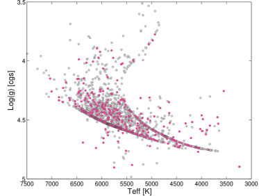
Figure 1 shows the ${\rm T_{\rm eff}}$ versus $\log{\rm g}$ stellar parameters for the Kepler planet candidate sample hosts. There is a clear concentration of stellar properties on the outer limits of the isochrones. This results from forcing the calculated stellar properties to match the closest isochrone available along with the fact that most stars were assumed to have a fixed metallicity of ${\rm[Fe/H]}$ $=-0.2$ . The targets with stellar properties that scatter outside the isochrone limits are targets for which no ${\rm T_{\rm eff}}$ is available from Pinsonneault et al. (2012), so the original KIC values were adopted (i.e. these were not fitted to the isochrones). The new Q1-Q8 Kepler planet candidate hosts (red circles) follow the distribution of stellar hosts to the previously identified planet candidates from (Borucki et al., 2011a, b; Batalha et al., 2013) (light gray circles), with a potential deficit in the sub-giant and giant gravity regimes.

Refer to caption — Figure 1.— Stellar surface gravity as a function of stellar effective temperature estimates for the targets hosting new Kepler planet candidates (red points). In addition, we show previously identified Kepler planet candidate hosts from Borucki et al. (2011a, b); Batalha et al. (2013) (gray points).

VI. Results

Table 1 reports the properties of the KOI stellar host and planet properties as described in § V and the KOI planet candidate or false positive designation following the procedure outlined in § IV. The table is comprehensive for all KOIs known as of this Q1-Q8 study. Table 1 reports the fitting of a limb-darkened transit model to the Kepler flux data resulting in the most direct geometric parameters: orbital period ( ${\rm P_{orb}}$ ), ephemeris epoch, transit model depth at closest approach, transit duration ( ${\rm T_{dur}}$ ), planet to star radius ratio ( ${\rm R_{P}}$ / ${\rm R_{\star}}$ ), impact parameter ( $b$ ), and semi-major axis to ${\rm R_{\star}}$ ratio ( $a$ / ${\rm R_{\star}}$ ). The resulting SNR of the transit model fit is also given in Table 1. Planet parameters for KOIs with a transit fit SNR $<$ 10 have an increasing possibility for systematic errors in the estimated parameters to become larger than the provided uncertainty estimates.

Table 1 reports the stellar host property estimates: stellar mass ( ${\rm M_{\star}}$ ), stellar radius ( ${\rm R_{\star}}$ ), effective temperature ( ${\rm T_{\rm eff}}$ ), and surface gravity ( $\log{\rm g}$ ). Combining the transit model geometric parameters with the stellar parameters yields the indirect planet properties: planet radius ( ${\rm R_{P}}$ ) and planet equilibrium temperature ( ${\rm T_{eq}}$ ) assuming a Bond albedo, $\alpha=0.3$ , and full surface redistribution of energy, $f=1.0$ . A more comprehensive table with additional parameters and parameter uncertainties is available in an interactive and searchable format from the NASA Exoplanet Archive as the Q1-Q8 activity table.

The disposition column (Disp) of Table 1 reports the status of a KOI as an integer where a value of 1 indicates a planet candidate and 2 indicates a false positive disposition, respectively. The newly dispositioned column (New KOI) of Table 1 indicates a binary flag which has a value 1 when the KOI was dispositioned with Q1-Q10 or more data products following the procedure outlined in this study (see § IV) and a value 0 when the KOI was excluded from dispositioning because the disposition status is adopted from Batalha et al. (2013), Bryson et al. (2013), or the KOI is a confirmed Kepler planet. The indeterminate period column in Table 1 indicates KOIs for which there is not a reliable period available since the flux time series only contains a single transit/eclipse event or the multiple events that are present do not enable uniquely assigning events to one or several candidates. The KOIs with a 1 in the indeterminate period column of Table 1 are subsequently not included in any statistical counts or figures for the rest of this paper as the information for these KOIs has considerable uncertainty.

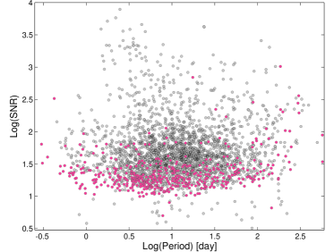
Figures 2-8 illustrate the properties of the Kepler planet candidate sample that is tabulated in Table 1 with the disposition flag, Disp=1. The new Kepler planet candidates identified in this study are indicated in the figures using red markers and the Kepler planet candidates identified in the earlier studies of Borucki et al. (2011a, b); Batalha et al. (2013) using light gray markers. Figure 2 shows the transit SNR (measured after detrending of the flux time series) resulting from the Q1-Q10 data limb-darkened transit model fits as a function of orbital period. The new Kepler planet candidates (red circles) are concentrated at low SNR relative to the previously identified Kepler planet candidates (gray circles). The rough floor in SNR is slightly elevated from the 7.1 threshold level, since the original detection being from Q1-Q8 data whereas the SNR is calculated from Q1-Q10 data. The population of high SNR planet candidates that are new discoveries arose for several reasons. At long periods, high SNR signals, even from a single transit event, previously did not have the requisite three transit events for detection in the pipeline. At short periods, high SNR detections occur for targets that were added to the observing sample in later observing quarters (typically as part of the Kepler Guest Observing program³³3http://keplerscience.arc.nasa.gov). The criteria (such as transit depth or obvious eclipsing binary signatures) for cataloging KOIs has varied through time. The pipeline software continues to develop increasing sensitivity.

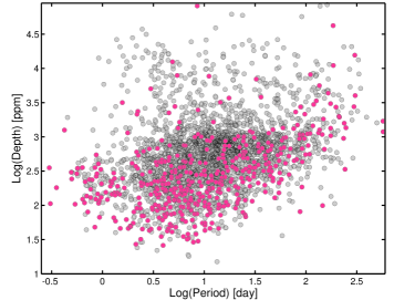
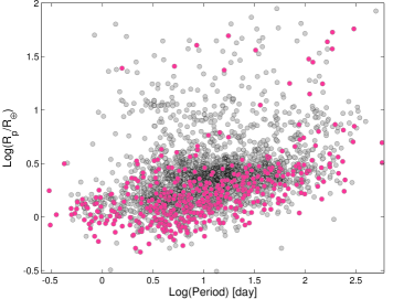
The left panel in Figure 3 shows the depth of transit (as measured from the best-fit transit model minimum relative flux) as a function of the orbital period. The new Kepler planet candidates identified in this study (red circles) populate a region of parameter space indicative of them being lower SNR detections (i.e. toward shallower depth and longer orbital period) than the previously identified Kepler planet candidates (light gray circles). Empirically, the sensitivity to planet candidates with a similar depth to 1 ${\rm R_{\oplus}}$ transiting in front of a 1 ${\rm R_{\odot}}$ host ( $\Delta$ =84 ppm) drops off considerably beyond a $\sim$ 30 day orbital period using Q1-Q8 Kepler data. The right panel in Figure 3 shows the Kepler planet candidate radii estimates (as measured from the best-fit transit model and stellar parameters described in § V) as a function of orbital period. Due to the presence of host stars of later-type than the Sun, the sensitivity to 1 ${\rm R_{\oplus}}$ planets extends to a longer orbital period and drops off strongly beyond a $\sim$ 55 day orbital period using Q1-Q8 Kepler data.

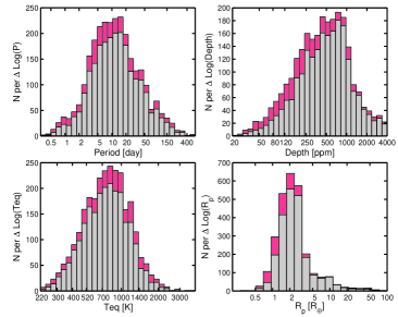
After re-evaluating the Kepler planet candidates from Borucki et al. (2011a, b), adopting the results of the Kepler planet sample from Batalha et al. (2013), and the 472 new Kepler planet candidates introduced in this study, there are 2,738 Kepler planet candidates in total. Thus, the new planet candidates increase the sample size by 21%. Figure 4 shows the distribution of the Kepler planet candidate sample in equal logarithmically spaced bins for the most interesting planet properties: orbital period, transit depth, radius, and equilibrium temperature, starting in the upper left panel and continuing clockwise, respectively. In each bin the red bar (on top) represents the count from the new planet candidates and the light gray bar (on bottom) represents the count from the previous planet candidate sample. The observed distribution of Kepler planet candidates represents the underlying planet distribution as shaped by the sensitivity of the Kepler instrument, pipeline planet search, and planet candidate evaluation process. We defer deriving the underlying planet population from Kepler planet candidate samples to future work (see § IV.4).

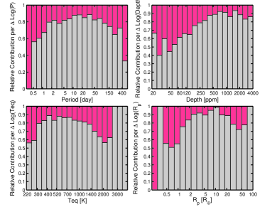
Due to their concentration toward low SNR (see Figure 2), the new planet candidates preferentially make a larger contribution to the small planet and long period distributions shown in Figure 4. In order to elucidate the contribution of the new planet candidates in parameter space, we complement the planet candidate distribution of Figure 4 by showing in Figure 5 the relative contribution of the new planet candidates and old planet candidates. For instance, of all Kepler planet candidates $\sim$ 40% with ${\rm R_{P}}$ $\sim$ 1 ${\rm R_{\oplus}}$ (lower right panel) are new in this study. For the cool ${\rm T_{eq}}$ $<$ 300 K Kepler planet candidates $\sim$ 40% are new in this study.

Multiple planet systems continue to be an important contribution to the Kepler planet candidate sample (Ford et al., 2011; Lissauer et al., 2011b; Fabrycky et al., 2012b). The 2,738 Kepler planet candidates are distributed amongst 2,017 stellar hosts. Of the planet candidate stellar hosts, 475 (23%) host multiple observed transiting planet candidates. Despite the multiple planet hosts being in the minority, their high observed multiplicity (up to 6) results in 1,196 (46%) of the planet candidates residing in multiple systems. The systems with 6 planet candidates are the confirmed system Kepler-11b-g (KOI 157 Lissauer et al., 2011a) and KOI 351.01-0.06. The left panel of Figure 6 shows the logarithm of the number of stellar hosts with planet candidates as a function of planet candidate multiplicity. The relative contribution of the new planet candidates to each multiplicity bin is shown in the right panel of Figure 6. The new planet candidates contribute a higher fraction of the rare, high multiplicity systems.

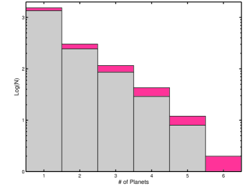
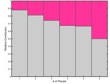
Figure 7 shows the planet candidate radius as a function of equilibrium temperature assuming an Earth-like Bond albedo, $\alpha=0.3$ , and redistribution of energy over the full surface. Horizontal lines indicate radii of the Solar System planets for reference, and the shaded vertical band indicates the adopted habitable zone (HZ) region for the possible existence of liquid water. Specifying the boundary of the HZ to support anthropocentrist life is an active area of research (Selsis et al., 2007; Kasting, 2011; Kopparapu et al., 2013; Zsom et al., 2013). In this study we adopt 180 $\leq$ ${\rm T_{eq}}$ $\leq$ 300 K as the HZ boundary based upon the guidance of Kasting (2011). The adoption of a sharp boundary for the HZ oversimplifies the complicated effects that can influence the ability for a planet to maintain a reservoir of liquid water (bulk planet composition, atmospheric composition, cloud and surface dynamics, etc.), and oversimplifies the significant observational uncertainty in equilibrium temperature for determining whether a planet lies in the HZ. However, since we only have the most basic information available about the planet candidate orbital period and stellar host properties the simplified HZ adopted here is sufficient for our purposes of providing descriptive statistics of the Kepler planet candidate sample.

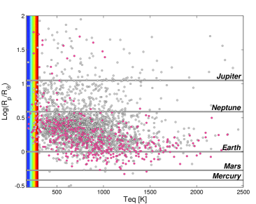
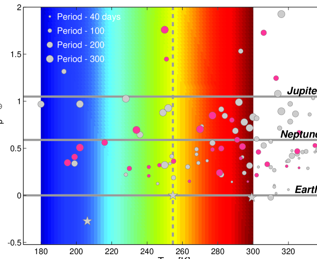
Figure 8 also shows the planet candidate radii as a function of equilibrium temperature, but details the narrow HZ region. The point size is proportional to the orbital period of the planet candidate. The largest point size corresponds to P $>$ 300 day and linearly decreases to the smallest point size corresponding to P $<$ 40 day. For fixed equilibrium temperature a larger point size indicates the planet candidate has a stellar host with an earlier spectral type. The vertical dashed line shows the ${\rm T_{eq}}$ =255 K for Earth. Star symbols indicate the Solar System planets Mars, Earth, & Venus from left to right, respectively. Overall, there are 57 HZ Kepler planet candidates of which 23 (40%) are new in this study. By adopting a more restrictive ${\rm T_{eq}}$ $<$ 270 K upper limit boundary to the HZ (Selsis et al., 2007), there are 32 HZ Kepler planet candidates of which 14 (44%) are new in this study.

From the set of new Kepler planet candidates in the HZ the three KOIs closest in radius and equilibrium temperature to Earth are KOI 172.02, 3010.01, and 1422.04. Subsequent to the first release of the new KOIs from this study at the NASA Exoplanet Archive⁴⁴4http://exoplanetarchive.ipac.caltech.edu/docs/tce_releasenotes_q1q12.pdf, KOI 172.02 was confirmed as Kepler-69c (Barclay et al., 2013). Of these three HZ KOIs new in this study, Kepler-69c has the longest orbital period, P=242 day, and orbits a Solar-type G4V host. The more detailed analysis of the Kepler-69 system (Barclay et al., 2013) yields a similar ${\rm R_{P}}$ =1.7 ${\rm R_{\oplus}}$ (versus ${\rm R_{P}}$ =1.74 ${\rm R_{\oplus}}$ ) and warmer ${\rm T_{eq}}$ =299 K (versus ${\rm T_{eq}}$ =281 K) planet than adopted in this study. KOI 3010.01 and 1422.04 orbit significantly cooler ${\rm T_{\rm eff}}$ $\sim$ 4000 K, and later ( ${\rm R_{\star}}$ $\sim$ 0.5 ${\rm R_{\odot}}$ ) spectral type hosts, and both have orbital periods $\sim$ 60 day. The planet candidate KOI 3010.01 has an estimated ${\rm R_{P}}$ =1.4 ${\rm R_{\oplus}}$ and ${\rm T_{eq}}$ =264 K. The planet candidate KOI 1422.04 has an estimated ${\rm R_{P}}$ =1.6 ${\rm R_{\oplus}}$ and ${\rm T_{eq}}$ =241 K.

VII. Conclusion

This study examines the potential planet candidate signals generated by the Kepler pipeline software searching Q1-Q8 ( $\sim$ 2 Years) of Kepler data. The Q1-Q8 search resulted in $\sim$ 13,400 targets with potential planet candidate signals, which was reduced to $\sim$ 480 new viable targets for planet candidate signals from an initial examination of the pipeline generated diagnostics (see § II). The viable planet candidates are assigned KOI numbers and undergo additional scrutiny in order to classify them into the Kepler planet candidate and false positive categories (see § IV).

In addition to the new Q1-Q8 KOIs, in this study we re-examined KOIs from the first two Kepler planet candidate samples (Borucki et al., 2011a, b) in order to take advantage of the substantially increased data baseline and a more uniform set of dispositioning criteria and procedures. Overall, between the new Q1-Q8 KOIs and re-evaluation of the Borucki et al. (2011a, b) KOIs, we classified $\sim$ 1,900 KOIs. To classify these two groups of KOIs we took advantage of improved pipeline data products and software using Q1-Q10 data. The total Kepler planet candidate sample reported in this study combines the new Q1-Q8 KOIs, the Borucki et al. (2011a, b) KOI sample re-evaluation, and the KOI sample and classification of Batalha et al. (2013), which is adopted without further scrutiny. Since the KOIs of Batalha et al. (2013) (evaluated with Q1-Q6 Kepler data) were not re-evaluated uniformly with the other KOIs (evaluated with Q1-Q10 Kepler data), the total Kepler planet candidate sample represents an inhomogeneous collection of the detections available with Kepler data making analysis of the underlying planet population from the reported planet candidates challenging (see § IV.4).

The current Kepler planet candidate sample provides researchers with a well vetted sample of individual planet candidates and new and expanded multiple planet candidate systems worthy of follow-up observations and scientific study. The total Kepler planet candidate sample count from this study is 2,738, with 472 (21%) new with the Q1-Q8 data analysis. The planet candidate gains are concentrated at lower SNR than the previous samples (see Figure 2); the new Q1-Q8 planet candidates contribute significantly ( $\sim$ 40%) to the population of the Kepler planet candidates having ${\rm R_{P}}$ $\sim$ 1 ${\rm R_{\oplus}}$ and to the population in the HZ of their stellar hosts. Multiple planet systems continue to be an important contribution to the Kepler planet candidate sample (Ford et al., 2011; Lissauer et al., 2011b; Fabrycky et al., 2012b). The 2,738 Kepler planet candidates are distributed amongst 2,017 stellar hosts. Despite the multiple planet hosts being in the minority (23% of all stellar hosts), their high observed multiplicity (up to 6) results in 46% of the planet candidates residing in multiple systems.

The Q1-Q8 Kepler planet candidate sample provides a rich population of objects which help elucidate the planet formation, planetary dynamics, stellar properties, and planet population statistics that govern the existence of planets in The Milky Way. We look forward to the expanded Kepler discoveries that follow from the Kepler planet candidates studied here along with the future discoveries enabled by the larger baseline (Q1-Q17) of the recently completed Kepler 3- and 4-wheel modes of operation.

Funding for this Discovery mission is provided by NASA’s Science Mission Directorate. MH and DH are supported by an appointment to the NASA Postdoctoral Program at Ames Research Center, administered by Oak Ridge Associated Universities through a contract with NASA.

Appendix A Additional KOI Vetting

This study specifically did not examine KOIs that were introduced in the KOI sample of Batalha et al. (2013). However, 220 KOIs were given false positive designations during the vetting of the planet candidate sample from Batalha et al. (2013), but these false positives were not published or documented. Because false positive identification techniques have improved since Batalha et al. (2013), we re-examined these 220 KOIs using the methods described in this paper. The data products used in the dispositioning were from a variety of pipeline runs (using $\geq$ Q1-Q10), and some of the KOIs required manual analysis of Kepler data. The column ‘Appendix KOI’ in Table 1 is a binary flag and indicates whether the KOI belongs to the group of 220 previously unpublished KOIs with an initial assessment as false positives. As indicated in the column ‘Disp’ in Table 1, 27 of these 220 KOIs have been restored to planet candidate status following their re-examination.

References

Aerts et al. (2010) Aerts, C., Christensen-Dalsgaard, J., & Kurtz, D. W. 2010, Asteroseismology, Astronomy and Astrophysics Library. ISBN 978-1-4020-5178-4. Springer Science+Business Media B.V., 2010
Barclay et al. (2013) Barclay, T., Burke, C. J., Howell, S. B., et al. 2013, ApJ, 768, 101
Batalha et al. (2011) Batalha, N. M., Borucki, W. J., Bryson, S. T., et al. 2011, ApJ, 729, 27
Batalha et al. (2013) Batalha, N. M., Rowe, J. F., Bryson, S. T., et al. 2013, ApJS, 204, 24
Batygin & Morbidelli (2013) Batygin, K., & Morbidelli, A. 2013, AJ, 145, 1
Borucki et al. (2010) Borucki, W. J., Koch, D., Basri, G., et al. 2010, Science, 327, 977
Borucki et al. (2011a) Borucki, W. J., Koch, D. G., Basri, G., et al. 2011, ApJ, 728, 117
Borucki et al. (2011b) Borucki, W. J., Koch, D. G., Basri, G., et al. 2011, ApJ, 736, 19
Borucki et al. (2012) Borucki, W. J., Koch, D. G., Batalha, N., et al. 2012, ApJ, 745, 120
Brown et al. (2011) Brown, T. M., Latham, D. W., Everett, M. E., & Esquerdo, G. A. 2011, AJ, 142, 112
Brown (2003) Brown, T. M. 2003, ApJ, 593, L125
Bryson et al. (2013) Bryson, S. T., Jenkins, J. M., Gilliland, R. L., et al. 2013, arXiv:1303.0052
Bryson et al. (2010) Bryson, S. T., Tenenbaum, P., Jenkins, J. M., et al. 2010, ApJ, 713, L97
Buchhave et al. (2012) Buchhave, L. A., Latham, D. W., Johansen, A., et al. 2012, Nature, 486, 375
Burke et al. (2006) Burke, C. J., Gaudi, B. S., DePoy, D. L., & Pogge, R. W. 2006, AJ, 132, 210
Burke (2008) Burke, C. J. 2008, ApJ, 679, 1566
Caldwell et al. (2010) Caldwell, D. A., van Cleve, J. E., Jenkins, J. M., et al. 2010, Proc. SPIE, 7731
Christiansen et al. (2012) Christiansen, J. L., Jenkins, J. M., Caldwell, D. A., et al. 2012, PASP, 124, 1279
Christiansen et al. (2013) Christiansen, J. L., Clarke, B. D., Burke, C. J., et al. 2013, arXiv:1303.0255
Claret & Bloemen (2011) Claret, A., & Bloemen, S. 2011, A&A, 529, A75
Dressing & Charbonneau (2013) Dressing, C. D., & Charbonneau, D. 2013, ApJ, 767, 95
Dunham et al. (2010) Dunham, E. W., Borucki, W. J., Koch, D. G., et al. 2010, ApJ, 713, L136
Endl et al. (2011) Endl, M., MacQueen, P. J., Cochran, W. D., et al. 2011, ApJS, 197, 13
Fabrycky et al. (2012a) Fabrycky, D. C., Ford, E. B., Steffen, J. H., et al. 2012, ApJ, 750, 114
Fabrycky et al. (2012b) Fabrycky, D. C., Lissauer, J. J., Ragozzine, D., et al. 2012, arXiv:1202.6328
Ford et al. (2011) Ford, E. B., Rowe, J. F., Fabrycky, D. C., et al. 2011, ApJS, 197, 2
Ford et al. (2012) Ford, E. B., Fabrycky, D. C., Steffen, J. H., et al. 2012, ApJ, 750, 113
Fressin et al. (2011) Fressin, F., Torres, G., Désert, J.-M., et al. 2011, ApJS, 197, 5
Fressin et al. (2013) Fressin, F., Torres, G., Charbonneau, D., et al. 2013, ApJ, 766, 81
Gautier et al. (2010) Gautier, T. N., III, Batalha, N. M., Borucki, W. J., et al. 2010, arXiv:1001.0352
Hansen & Murray (2013) Hansen, B., & Murray, N. 2013, arXiv:1301.7431
Hébrard et al. (2013) Hébrard, G., Almenara, J.-M., Santerne, A., et al. 2013, A&A, 554, A114
Holman et al. (2010) Holman, M. J., Fabrycky, D. C., Ragozzine, D., et al. 2010, Science, 330, 51
Howard et al. (2012) Howard, A. W., Marcy, G. W., Bryson, S. T., et al. 2012, ApJS, 201, 15
Huber et al. (2013) Huber, D., Chaplin, W. J., Christensen-Dalsgaard, J., et al. 2013, ApJ, 767, 127
Jenkins (2002) Jenkins, J. M. 2002, ApJ, 575, 493
Jenkins et al. (2010) Jenkins, J. M., Caldwell, D. A., Chandrasekaran, H., et al. 2010, ApJ, 713, L87
Jenkins et al. (2013) Jenkins, J. M., Christiansen, J., Burke, C. J., et al. 2013, American Astronomical Society Meeting Abstracts, 221, #216.04
Kasting (2011) Kasting, J. F. 2011, Joint Meeting of the Exoplanet and Cosmic Origins Program Analysis Groups (ExoPAG and COPAG), April 26, 2011, Baltimore, MD, http://exep.jpl.nasa.gov/exopag/exopagCopagJointMeeting/
Kolodziejczak et al. (2010) Kolodziejczak, J. J., Caldwell, D. A., van Cleve, J. E., et al. 2010, Proc. SPIE, 7742,
Kopparapu et al. (2013) Kopparapu, R. K., Ramirez, R., Kasting, J. F., et al. 2013, ApJ, 765, 131
Latham et al. (2010) Latham, D. W., Borucki, W. J., Koch, D. G., et al. 2010, ApJ, 713, L140
Lissauer et al. (2011a) Lissauer, J. J., Fabrycky, D. C., Ford, E. B., et al. 2011, Nature, 470, 53
Lissauer et al. (2011b) Lissauer, J. J., Ragozzine, D., Fabrycky, D. C., et al. 2011, ApJS, 197, 8
Mandel & Agol (2002) Mandel, K., & Agol, E. 2002, ApJ, 580, L171
Morton & Johnson (2011) Morton, T. D., & Johnson, J. A. 2011, ApJ, 738, 170
Pinsonneault et al. (2012) Pinsonneault, M. H., An, D., Molenda-Żakowicz, J., et al. 2012, ApJS, 199, 30
Prša et al. (2011) Prša, A., Batalha, N., Slawson, R. W., et al. 2011, AJ, 141, 83
Rein (2012) Rein, H. 2012, MNRAS, 427, L21
Ricker et al. (2010) Ricker, G. R., Latham, D. W., Vanderspek, R. K., et al. 2010, Bulletin of the American Astronomical Society, 42, #450.06
Rowe et al. (2006) Rowe, J. F., Matthews, J. M., Seager, S., et al. 2006, ApJ, 646, 1241
Santerne et al. (2011) Santerne, A., Díaz, R. F., Bouchy, F., et al. 2011, A&A, 528, A63
Schmidt-Kaler (1982) Schmidt-Kaler, T. 1982, in Landolt-Bornstein New Series, Group 6, Vol. 2b, Stars and Star Clusters, ed. K. Schaifers & H.-H. Voigt (Berlin: Springer)
Selsis et al. (2007) Selsis, F., Kasting, J. F., Levrard, B., et al. 2007, A&A, 476, 1373
Sirko & Paczyński (2003) Sirko, E., & Paczyński, B. 2003, ApJ, 592, 1217
Slawson et al. (2011) Slawson, R. W., Prša, A., Welsh, W. F., et al. 2011, AJ, 142, 160
Smith et al. (2012) Smith, J. C., Stumpe, M. C., Van Cleve, J. E., et al. 2012, PASP, 124, 1000
Steffen et al. (2012) Steffen, J. H., Fabrycky, D. C., Ford, E. B., et al. 2012, MNRAS, 421, 2342
Stumpe et al. (2012) Stumpe, M. C., Smith, J. C., Van Cleve, J. E., et al. 2012, PASP, 124, 985
Skrutskie et al. (2006) Skrutskie, M. F., Cutri, R. M., Stiening, R., et al. 2006, AJ, 131, 1163
Tenenbaum et al. (2012) Tenenbaum, P., Christiansen, J. L., Jenkins, J. M., et al. 2012, ApJS, 199, 24
Tenenbaum et al. (2013) Tenenbaum, P., Jenkins, J. M., Seader, S., et al. 2012, arXiv:1212.2915
Thompson et al. (2012) Thompson, S. E., Everett, M., Mullally, F., et al. 2012, ApJ, 753, 86
Torres et al. (2004) Torres, G., Konacki, M., Sasselov, D. D., & Jha, S. 2004, ApJ, 614, 979
Torres et al. (2011) Torres, G., Fressin, F., Batalha, N. M., et al. 2011, ApJ, 727, 24
Twicken et al. (2010a) Twicken, J. D., Chandrasekaran, H., Jenkins, J. M., et al. 2010, Proc. SPIE, 62, 7740
Twicken et al. (2010b) Twicken, J. D., Clarke, B. D., Bryson, S. T., et al. 2010, Proc. SPIE, 69, 7740
Valenti & Piskunov (1996) Valenti, J. A., & Piskunov, N. 1996, A&AS, 118, 595
Wang et al. (2013) Wang, J., Fischer, D. A., Barclay, T., et al. 2013, ApJ, 776, 10
Wielen (1996) Wielen, R. 1996, A&A, 314, 679
Wu et al. (2010) Wu, H., Twicken, J. D., Tenenbaum, P., et al. 2010, Proc. SPIE, 7740
Xie (2013) Xie, J.-W. 2013, ApJS, 208, 22
Yi et al. (2001) Yi, S., Demarque, P., Kim, Y.-C., et al. 2001, ApJS, 136, 417
Youdin (2011) Youdin, A. N. 2011, ApJ, 742, 38
Zsom et al. (2013) Zsom, A., Seager, S., de Wit, J., & Stamenkovic, V. 2013, arXiv:1304.3714

Table 1KOI Ephemeris, Planet Parameters, Stellar Parameters, & Disposition Status^a^aA version of the Table with comprehensive reporting of parameters and their uncertainties is published in the Q1-Q8 KOI activity table at the NASA Exoplanet Archive http://exoplanetarchive.ipac.caltech.edu

KOI	Kepler Id	${\rm P_{orb}}$	Epoch^b^bBJD=Epoch+2454900.0	Depth	a/ ${\rm R_{\star}}$	b	${\rm T_{dur}}$	${\rm R_{P}}$ / ${\rm R_{\star}}$	SNR	${\rm R_{\star}}$	${\rm M_{\star}}$	${\rm T_{\rm eff}}$	$\log{\rm g}$	${\rm R_{P}}$	Teq	Disp^c^cDisposition ; 1 = Planet Candidate ; 2 = False Positive	New^d^dNew KOI to Kepler Q1-Q8 sample ; 1 = True ; 0 = False	Appendix^e^eKOI from Appendix A. ; 1 = True ; 0 = False	Disp^f^fDisposition for KOI was updated during this study ; 1 = True ; 0 = False	Indeterminate^g^gSingle transit or ambiguous period KOI ; 1 = True ; 0 = False	KIC^h^hStellar parameters unclassified in the Kepler Input Catalog ; 1 = True ; 0 = False
		$[$ day $]$		$[$ ppm $]$			$[$ hr $]$			$[$ ${\rm R_{\odot}}$ $]$	$[$ ${\rm M_{\odot}}$ $]$	$[$ K $]$	$[$ cgs $]$	$[$ ${\rm R_{\oplus}}$ $]$	$[$ K $]$		KOI	KOI	This Study	Period	unclassified
1.01	11446443	2.470613	55.762566	14284.0	8.445	0.8222	1.725	0.12437	7856.10	1.06	0.99	5814.0	4.381	14.45	1394.0	1	0	0	0	0	0
2.01	10666592	2.204735	54.357802	6713.0	4.681	0.1282	3.877	0.07545	5812.40	2.71	1.66	6264.0	3.792	22.32	2303.0	1	0	0	0	0	0
3.01	10748390	4.887800	57.812537	4323.0	16.681	0.0286	2.368	0.05770	1433.40	0.74	0.79	4766.0	4.592	4.68	794.0	1	0	0	0	0	0
4.01	3861595	3.849372	90.525922	1340.0	4.481	0.9462	2.928	0.04152	284.00	2.60	1.61	6391.0	3.812	11.81	1923.0	2	0	0	1	0	0
5.01	8554498	4.780329	65.973245	966.0	7.560	0.9507	2.012	0.03651	456.20	1.42	1.15	5861.0	4.193	5.66	1279.0	1	0	0	1	0	0
…
3145.02	1717722	0.977314	64.698560	207.0	5.032	0.0307	1.262	0.01461	11.10	0.63	0.72	4771.0	4.690	1.01	1284.0	1	1	0	1	0	0
3146.01	10908248	39.859247	87.772400	157.0	36.775	0.0261	8.355	0.01110	14.30	1.08	0.97	5900.0	4.353	1.31	570.0	1	1	0	1	0	0
3147.01	7534267	39.441307	102.146160	197.0	42.945	0.0416	7.098	0.01246	17.00	0.86	0.97	5765.0	4.554	1.17	499.0	1	1	0	1	0	0
3148.01	10611420	11.505399	68.098080	288.0	26.146	0.6919	2.500	0.01657	14.30	1.07	1.15	6354.0	4.438	1.94	896.0	2	1	0	1	0	0
3149.01	10196493	9.811017	67.186760	61.0	16.959	0.8950	2.086	0.00868	4.80	1.00	0.94	5799.0	4.406	0.95	864.0	2	1	0	1	0	0

Note. — Table published in its entirety in the journal electronic addition. A portion is displayed here to illustrate its form and content.