Simulated star formation rate functions at $\bf{z\sim 4-7}$, and the role of feedback in high-$\bf{z}$ galaxies

Abstract

We study the role of feedback from supernovae and black holes in the evolution of the star formation rate function (SFRF) of $z\sim 4-7$ galaxies. We use a new set of cosmological hydrodynamic simulations, Angus (AustraliaN GADGET-3 early Universe Simulations), run with a modified and improved version of the parallel TreePM-smoothed particle hydrodynamics code GADGET-3 called P-GADGET3(XXL), that includes a self-consistent implementation of stellar evolution and metal enrichment. In our simulations both Supernova (SN) driven galactic winds and Active Galactic Nuclei (AGN) act simultaneously in a complex interplay. The SFRF is insensitive to feedback prescription at $z>5$, meaning that it cannot be used to discriminate between feedback models during reionisation. However, the SFRF is sensitive to the details of feedback prescription at lower redshift. By exploring different SN driven wind velocities and regimes for the AGN feedback, we find that the key factor for reproducing the observed SFRFs is a combination of “strong” SN winds and early AGN feedback in low mass galaxies. Conversely, we show that the choice of initial mass function and inclusion of metal cooling have less impact on the evolution of the SFRF. When variable winds are considered, we find that a non-aggressive wind scaling is needed to reproduce the SFRFs at $z\apprge 4$. Otherwise, the amount of objects with low SFRs is greatly suppressed and at the same time winds are not effective enough in the most massive systems.

1 Introduction

A detailed understanding of galaxy formation and evolution in the cold dark matter model remains a challenge for modern cosmology, especially at high redshift. The star formation history is determined by a complex interplay of gas accretion onto the potential wells created by the Dark Matter (DM) halos, star formation and associated feedback processes. Cosmological simulations have become a powerful tool to study how these astrophysical phenomena interact and influence each other (Schaye et al., 2010; Finlator et al., 2011; Davé et al., 2011; Maio et al., 2011; Choi & Nagamine, 2012; Jaacks et al., 2012; Puchwein & Springel, 2013; Wilkins et al., 2013; Kannan et al., 2013; Vogelsberger et al., 2013). However, despite the incredible growth of available computating resources seen in recent years (in terms of both hardware and software), numerical codes that follow both dark matter and baryonic physics still have shortcomings, mainly because of the complexity and the different range of scales of the physics involved. It is, for example, numerically infeasible to fully resolve all the relevant processes that govern the formation of stars in galaxies and their backreaction on the interstellar medium (Puchwein & Springel, 2013). For this reason, current cosmological simulations use sub-resolution schemes to model the physics of star formation, supernova explosions and black hole gas accretion. On the other hand, numerical techniques have been substantially improved during the last few years (e.g. Murante et al., 2011; Read & Hayfield, 2012; Hopkins, 2013). Particularly interesting is the moving mesh approach, since it combines the best features of grid and particle based codes (Springel, 2010; Sijacki et al., 2012; Kereš et al., 2012; Vogelsberger et al., 2012; Torrey et al., 2012; Nelson et al., 2013; Vogelsberger et al., 2013).

Observationally, our knowledge of Star Formation Rates (SFRs) and stellar masses in the distant Universe has expanded substantially over the last several years thanks to deep multi-wavelength surveys (Bernardi et al., 2010; González et al., 2011; Lee et al., 2012; Smit et al., 2012; Santini et al., 2012; Bouwens et al., 2012; Schenker et al., 2012). In particular, the evolution of the star formation rate over cosmic time is a fundamental constraint for theories of galaxy formation and evolution (Hopkins, 2004; Wilkins et al., 2008; Guo et al., 2011; Cucciati et al., 2012; Bouwens et al., 2012). Furthermore, Star Formation Rate Functions (SFRFs) provide a physical description of galaxy buildup at high redshift. In a recent work, Smit et al. (2012) combined the UV luminosity functions of Bouwens et al. (2007, 2011) with new estimates of dust extinction, to derive the SFRF of $z\sim 4-7$ galaxies. Their results provide strong indications that galaxies build up uniformly over the first 3 Gyr of the Universe.

The star formation rate functions at lower redshift have been studied by means of both simulations (Davé et al., 2011) and semi-analytic models (Fontanot et al., 2012). In particular, Davé et al. (2011) used a set of simulations run with an extended version of the hydrodynamic code GADGET-2 to study the growth of the stellar content of galaxies at redshift $0\leq z\leq 3$. The authors implemented four different wind models and simulated stellar mass and star formation rate functions to quantify the effects of outflows on galactic evolution. In their simulations, galactic winds are responsible for the shape of the faint end slope of the SFR function at $z=0$. However, feedback from Active Galactic Nuclei (AGN) is not taken into account and, as a result, their simulations overproduce the number of objects in the high star formation rate tail. Puchwein & Springel (2013), instead, used GADGET-3 to investigate how both supernova and AGN feedback processes affect the shape of the galaxy stellar mass functions (GSMFs) at redshift $0\leq z\leq 2$. These authors suggest that an energy-driven wind model in which the wind velocity decreases and the wind mass loading increases in low mass galaxies (Martin, 2005), can produce a good match to the low mass end of the observed GSMF. Conversely, the high mass end can be recovered simultaneously if AGN feedback is included. The importance of AGN feedback in shaping the high end of the luminosity functions at low redshift is also indicated by semi-analytic models (Croton et al., 2006; Bower et al., 2006).

The aim of this work is to investigate the relative importance of galactic winds and AGN feedback at higher redshift. We use state-of-the-art cosmological hydrodynamic simulations run with a modified and improved version of the widely used Smoothed Particle Hydrodynamics (SPH) code GADGET-3 (last described in Springel, 2005) called P-GADGET3(XXL). As a first scientific case, in this paper we study the evolution of the star formation rate function of high redshift galaxies. In a companion paper (Katsianis et al., 2013) we will explore the stellar mass function and the star formation rate$-$stellar mass relation for high redshift galaxies.

The paper is organized as follows. In Sections 2.1 and 2.2 we present the hydrodynamic code P-GADGET3(XXL) and our simulation project Angus. In Section 2.3 we discuss the different feedback models included in our runs and in Section 2.4 we describe the characteristics of the simulations used in this work. In Section 3 we study the evolution of the cosmic star formation rate density. In Section 4.1 we summarise observations of the star formation rate function of high redshift galaxies from Smit et al. (2012), and compare with our simulations in Section 4.2. In Section 5 we discuss our main results, and present conclusions in Section 6.

2 The simulations

The set of simulations used in this work is part of the AustraliaN GADGET-3 early Universe Simulations (Angus) project. We have started this project to study the interplay between galaxies and the Intergalactic Medium (IGM) from low redshift ($z<2$) to the epoch of reionisation at $z\sim 6$ and above.

2.1 The code

P-GADGET3(XXL) (PG3) is an improved version of GADGET-3 (Springel, 2005). For the first time it combines a number of physical processes, which have been developed and tested separately. In particular, for this work we used:

• a sub-grid star formation model (Springel & Hernquist, 2003);

• self-consistent stellar evolution and chemical enrichment modeling (Tornatore et al., 2007);

• supernova energy- and momentum-driven galactic winds (Springel & Hernquist, 2003; Puchwein & Springel, 2013);

• AGN feedback (Springel et al., 2005; Fabjan et al., 2010; Planelles et al., 2012);

• metal-line cooling (Wiersma et al., 2009);

• a low-viscosity SPH scheme to allow the development of turbulence within the intracluster medium (Dolag et al., 2005).

Additional physical modules will be explored in the future:

• new supernova driven galactic wind feedback prescriptions (Barai et al., 2013);

• transition of metal free Population III to Population II star formation (Tornatore et al., 2007b);

• low-temperature cooling by molecules/metals (Maio et al., 2007);

• adaptive gravitational softening (Iannuzzi & Dolag, 2011);

• thermal conduction (Dolag et al., 2004);

• passive magnetic fields based on Euler potentials (Dolag & Stasyszyn, 2009).

Moreover, the following on the fly tools have been added to PG3:

• parallel Friends-of-Friends (FoF) algorithm to identify collapsed structures. The FoF links over all particle types (dark matter, gas and stars), and enables combinations of one, two or three types. Following Dolag et al. (2009), we use a linking length of 0.16 times the mean DM particle separation;

• parallel SUBFIND algorithm to identify substructures within FoF halos (Springel et al., 2001; Dolag et al., 2009). The formation of purely gaseous substructures is prevented and, if the Chabrier (2003) Initial Mass Function (IMF) is used, SUBFIND can assign luminosities in 12 bands (u, V, G, r, i, z, Y, J, H, K, L, M) to subhalos, including dust attenuation (based on spectral energy distributions from Charlot & Bruzual in preparation).

PG3 is currently being used for a range of different scientific projects, including study of galaxy clusters and magnetic fields within the large scale structures.

2.2 The ANGUS project

We have performed a set of cosmological simulations assuming a flat $\Lambda$CDM model with $\Omega_{\rm 0m}=0.272$, $\Omega_{\rm 0b}=0.0456$, $\Omega_{\rm\Lambda}=0.728$, $n_{\rm s}=0.963$, $H_{\rm 0}=70.4$ km s^-1 Mpc^-1 (or $h=0.704$) and $\sigma_{\rm 8}=0.809$. This set of cosmological parameters is the combination of 7-year data from WMAP (Komatsu et al., 2011) with the distance measurements from the baryon acoustic oscillations in the distribution of galaxies (Percival et al., 2010) and the Hubble constant measurement of Riess et al. (2009).

Each simulation produces a cosmological box with periodic boundary conditions and initially contains an equal number of gas and dark matter particles. We adopt the multiphase star formation criterion of Springel & Hernquist (2003), where a prescription for the Interstellar Medium (ISM) is included. In this model, the ISM is represented as a fluid comprised of cold condensed clouds in pressure equilibrium with an ambient hot gas. The clouds supply the material available for star formation. Whenever the density of a gas particle exceeds a given threshold $\rho_{\rm th}$, that gas particle is flagged as star forming and is treated as multiphase. With this prescription, baryons are in the form of either a hot or a cold phase or in stars, so that this density threshold marks the onset of cold cloud formation. Mass exchange between the different phases is driven by the effect of star formation, cloud evaporation and cooling. A typical value for $\rho_{\rm th}$ is $\sim 0.1$ cm^-3 (in terms of the number density of hydrogen atoms), but the exact density threshold is calculated according to the IMF used and the inclusion/exclusion of metal-line cooling (see below). This guarantees that our simulations generate the Kennicutt-Schmidt law (Kennicutt, 1998) by construction.

PG3 self-consistently follows the evolution of hydrogen, helium and 9 metallic species (C, Ca, O, N, Ne, Mg, S, Si and Fe) released from Supernovae (SNIa and SNII) and Low and Intermediate Mass Stars (LIMSs). Radiative cooling and heating processes are included following the procedure presented in Wiersma et al. (2009). We assume a mean background radiation composed of the cosmic microwave background and the Haardt & Madau (2001) ultraviolet/X-ray background from quasars and galaxies. Contributions to cooling from each of the eleven elements mentioned above have been pre–computed using the Cloudy photo–ionisation code (last described in Ferland et al., 2013) for an optically thin gas in (photo)ionisation equilibrium. In this work we use cooling tables for gas of primordial composition (H $+$ He) as the reference configuration. To test the effect of metal-line cooling, we include it in one simulation. It is worth noting that this procedure for computing cooling rates allows us to relax the assumptions of collisional ionisation equilibrium and solar relative abundances of the elements previously adopted (Tornatore et al., 2007; Tescari et al., 2009, 2011). Mixing and diffusion are not included in our simulations. However, to make sure that metals ejected by stars in the ISM mix properly, for each gas particle in the ISM we consider a “smoothed metallicity” calculated taking into account the contribution of neighbouring SPH particles. This procedure effectively reduces the noise associated with the lack of diffusion and mixing.

Our model of chemical evolution accounts for the age of various stellar populations and metals, which are released over different time scales by stars of different mass. We adopt the lifetime function of Padovani & Matteucci (1993) and the following stellar yields:

• SNIa: Thielemann et al. (2003). The mass range for the SNIa originating from binary systems is 0.8 M${}_{\rm\odot}<m\leq 8$ M_⊙, with a binary fraction of 7 per cent.

• SNII: Woosley & Weaver (1995). The mass range for the SNII is $m>8$ M_⊙.

• LIMS: van den Hoek & Groenewegen (1997).

In the code, every star particle represents a Simple Stellar Population (SSP). To describe this SSP, we take into account stars with mass in the interval 0.1 M${}_{\rm\odot}\leq m\leq 100$ M_⊙. Only stars with mass $m\leq 40$ M_⊙ explode as SN before turning into black holes, while stars of mass $m>40$ M_⊙ collapse directly to a black hole without forming a SN.

An important ingredient of the model is the initial stellar mass function $\xi(m)$, which defines the distribution of stellar masses (dN) per logarithmic mass interval that form in one star formation event in a given volume of space:

$$\xi(m)=\frac{{\rm d}\,{\rm N}}{{\rm d}\log m}.$$ (1)

The most widely used functional form for the IMF is the power law, as suggested originally by Salpeter (1955):

$$\xi(m)=A\,m^{-x},$$ (2)

where $A$ is a normalization factor, set by the condition:

$$\int_{m_{\rm inf}}^{m_{\rm sup}}\xi(m)\,{\rm d}m=1,$$ (3)

where in our case $m_{\rm inf}=0.1$ M_⊙ and $m_{\rm sup}=100$ M_⊙. In this work we use three different initial stellar mass functions:

• Salpeter (1955): single sloped,

  $$\xi(m)=0.172\times m^{-1.35}$$ (4)

• Kroupa et al. (1993): multi sloped,

  $$\xi(m)=\left\{\begin{array}[]{l}0.579\times m^{-0.3}\ \ 0.1\,{\rm M}_{\rm\odot}\leq m<0.5\,{\rm M}_{\rm\odot}\\ 0.310\times m^{-1.2}\ \ 0.5\,{\rm M}_{\rm\odot}\leq m<1\,{\rm M}_{\rm\odot}\\ 0.310\times m^{-1.7}\ \ m\geq 1\,{\rm M}_{\rm\odot}\end{array}\right.$$ (8)

• Chabrier (2003): multi sloped,

  $$\xi(m)=\left\{\begin{array}[]{l}0.497\times m^{-0.2}\ \ 0.1\,{\rm M}_{\rm\odot}\leq m<0.3\,{\rm M}_{\rm\odot}\\ 0.241\times m^{-0.8}\ \ 0.3\,{\rm M}_{\rm\odot}\leq m<1\,{\rm M}_{\rm\odot}\\ 0.241\times m^{-1.3}\ \ m\geq 1\,{\rm M}_{\rm\odot}\end{array}\right.$$ (12)

The initial mass function is particularly important, because the stellar mass distribution determines the evolution, surface brightness, chemical enrichment, and baryonic content of galaxies. The shape of the IMF also determines how many long-lived stars form with respect to massive short-lived stars. In turn, this ratio affects the amount of energy released by SN and the current luminosity of galaxies which is dominated by low-mass stars. The Salpeter IMF predicts a larger number of low-mass stars, while the Kroupa and the Chabrier IMFs predict a larger number of intermediate and high-mass stars, respectively. However, note that we neglect the effect of assuming different IMFs on the observationally inferred cosmic SFR. Therefore, the choice of the IMF has an indirect (minor) impact on the evolution of the cosmic star formation rate density and on the star formation rate functions, as we discuss in Section 3 and 4.2, respectively. Conversely, the same choice produces different enrichment patterns as shown in Tornatore et al. (2007).

2.3 Feedback models

In our simulations both SN driven galactic winds and AGN feedback act simultaneously in a complex interplay. In one run we adopt variable momentum-driven galactic winds, while all the other simulations include energy-driven galactic winds of constant velocity. In the following sub-sections we discuss our different feedback models.

2.3.1 Energy-driven galactic winds

We use the Springel & Hernquist (2003) implementation of energy-driven galactic winds. The wind mass-loss rate ($\dot{\rm M}_{\rm w}$) is assumed to be proportional to the star formation rate ($\dot{\rm M}_{\rm\star}$) according to:

$$\dot{\rm M}_{\rm w}=\eta\dot{\rm M}_{\rm\star},$$ (13)

where the wind mass loading factor $\eta$ is a parameter that accounts for the wind efficiency. The wind carries a fixed fraction $\chi$ of the SN energy $\epsilon_{\rm SN}$:

$$\frac{1}{2}\dot{\rm M}_{\rm w}v_{\rm w}^{2}=\chi\,\epsilon_{\rm SN}\dot{\rm M}_{\rm\star}\,\,\,\,\Longrightarrow\,\,\,\,v_{\rm w}=\sqrt{\frac{2\,\chi\,\epsilon_{\rm SN}}{\eta}},$$ (14)

where $v_{\rm w}$ is the wind velocity. Star-forming gas particles are then stochastically selected according to their SFR to become part of a blowing wind. Whenever a particle is uploaded to the wind, it is decoupled from the hydrodynamics for a given period of time. The maximum allowed time for a wind particle to stay hydrodynamically decoupled is $t_{\rm dec}=l_{\rm w}/v_{\rm w}$, where $l_{\rm w}$ is the wind free travel length. In addition, when $t<t_{\rm dec}$, a wind particle will re-couple to the hydrodynamics as soon as it reaches a region with a density:

$$\rho<\delta_{\rm w}\rho_{\rm th},$$ (15)

where $\rho_{\rm th}$ is the density threshold for the onset of the star formation and $\delta_{\rm w}$ is the wind free travel density factor. The parameters $t_{\rm dec}$ and $\delta_{\rm w}$ have been introduced in order to prevent a gas particle from getting trapped into the potential well of the virialized halo, thus allowing effective escape from the ISM into the low-density IGM.

We consider the velocity of the wind $v_{\rm w}$ as a free parameter (Tornatore et al., 2010). The following additional parameters therefore fully specify the wind model: $\eta=2$ (Martin, 1999), $t_{\rm dec}=0.025\left[\frac{{\rm comoving\ kpc}/h}{{\rm km/s}}\right]$ (code internal units corresponding to $\sim 34.7$ Myr) and $\delta_{\rm w}=0.5$ ($\chi$ being fixed by the choice of $v_{\rm w}$). In this work we explore three different values of $v_{\rm w}$:

• weak winds: $v_{\rm w}=350$ km/s. Since in code internal units $t_{\rm dec}=l_{\rm w}/v_{\rm w}=0.025\left[\frac{{\rm comoving\ kpc}/h}{{\rm km/s}}\right]$, in this case the wind free travel length is $l_{\rm w}=8.75$ kpc/$h$ (comoving);

• strong winds: $v_{\rm w}=450$ km/s ($l_{\rm w}=11.25$ kpc/$h$);

• very strong winds: $v_{\rm w}=550$ km/s ($l_{\rm w}=13.75$ kpc/$h$).

2.3.2 Momentum-driven galactic winds

To test the sensitivity of our conclusions to the adopted wind model, we performed a simulation that includes variable winds. According to the observational results of Martin (2005), we assume that in a given halo the velocity of the wind depends on the mass of the halo M_halo:

$$v_{\rm w}=2\;\sqrt{\frac{G{\rm M}_{\rm halo}}{R_{\rm 200}}}=2\times v_{\rm circ},$$ (16)

where $v_{\rm circ}$ is the circular velocity and $R_{\rm 200}$ is the radius within which a density 200 times the mean density of the Universe at redshift $z$ is enclosed (Barai et al., 2013):

$$R_{\rm 200}=\sqrt[3]{\frac{3}{4\pi}\frac{{\rm M}_{\rm halo}}{200\rho_{\rm c}\Omega_{\rm 0m}}}\left(1+z\right)^{-1}.$$ (17)

In this equation $\rho_{\rm c}=3H_{\rm 0}^{2}/(8\pi G)$ is the critical density at $z=0$. Following Puchwein & Springel (2013), we consider a momentum-driven scaling of the wind mass loading factor:

$$\eta=2\times\frac{450\,\,{\rm km/s}}{v_{\rm w}},$$ (18)

where $\eta=2$ if the wind velocity is equal to our reference constant (strong) wind model $v_{\rm w}=450$ km/s. Here again, we decouple wind particles from the hydrodynamics for a given period of time.

Besides the kinetic (energy- or momentum-driven) feedback just described, contributions from both SNIa and SNII to thermal feedback are also considered.

	Run	IMF	Box Size	NTOT	MDM	MGAS	Comoving Softening	Feedback
			[Mpc/$h$]		[M⊙/$h$]	[M⊙/$h$]	[kpc/$h$]
	Kr24_eA_sW	Kroupa	24	$2\times 288^{3}$	3.64$\times 10^{7}$	$7.32\times 10^{6}$	4.0	Early AGN $+$ Strong Winds
	Ch24_lA_wW	Chabrier	24	$2\times 288^{3}$	3.64$\times 10^{7}$	$7.32\times 10^{6}$	4.0	Late AGN $+$ Weak Winds
	Sa24_eA_wW	Salpeter	24	$2\times 288^{3}$	3.64$\times 10^{7}$	$7.32\times 10^{6}$	4.0	Early AGN $+$ Weak Winds
	Ch24_eA_sW	Chabrier	24	$2\times 288^{3}$	3.64$\times 10^{7}$	$7.32\times 10^{6}$	4.0	Early AGN $+$ Strong Winds
	Ch24_lA_sW	Chabrier	24	$2\times 288^{3}$	3.64$\times 10^{7}$	$7.32\times 10^{6}$	4.0	Late AGN $+$ Strong Winds
	Ch24_eA_vsW	Chabrier	24	$2\times 288^{3}$	3.64$\times 10^{7}$	$7.32\times 10^{6}$	4.0	Early AGN $+$ Very Strong Winds
	Ch24_NF	Chabrier	24	$2\times 288^{3}$	3.64$\times 10^{7}$	$7.32\times 10^{6}$	4.0	No Feedback
	Ch24_Zc_eA_sWa	Chabrier	24	$2\times 288^{3}$	3.64$\times 10^{7}$	$7.32\times 10^{6}$	4.0	Early AGN $+$ Strong Winds
	Ch24_eA_MDWb	Chabrier	24	$2\times 288^{3}$	3.64$\times 10^{7}$	$7.32\times 10^{6}$	4.0	Early AGN $+$
								Momentum-Driven Winds
	Ch18_lA_wW	Chabrier	18	$2\times 384^{3}$	6.47$\times 10^{6}$	$1.30\times 10^{6}$	2.0	Late AGN $+$ Weak Winds
	Ch12_eA_sW	Chabrier	12	$2\times 384^{3}$	1.92$\times 10^{6}$	$3.86\times 10^{5}$	1.5	Early AGN $+$ Strong Winds

Table 1: Summary of the different runs used in this work. Column 1, run name; column 2, Initial Mass Function (IMF) chosen; column 3, box size in comoving Mpc/$h$; column 4, total number of particles (N${}_{\rm TOT}=$ N_GAS $+$ N_DM); column 5, mass of the dark matter particles; column 6, initial mass of the gas particles; column 7, Plummer-equivalent comoving gravitational softening length; column 8, type of feedback implemented. See Section 2.4 for more details on the parameters used for the different feedback recipes. $(a)$: in this simulation the effect of metal-line cooling is included (Section 2.2). $(b)$: in this simulation we adopt variable momentum-driven galactic winds. In all the other simulations galactic winds are energy-driven and the wind velocity is constant. (Section 2.3).

2.3.3 AGN feedback

Our model for AGN feedback is based on the implementation proposed by Springel et al. (2005), with feedback energy released from gas accretion onto Super-Massive Black Holes (SMBHs). However, our model introduces some modifications (Fabjan et al., 2010; Planelles et al., 2012). SMBHs are described as collisionless sink particles initially seeded in dark matter halos, which grow via gas accretion and through mergers with other SMBHs during close encounters. Whenever a dark matter halo, identified by the parallel run-time FoF algorithm, reaches a mass above a given mass threshold M_th for the first time, it is seeded with a central SMBH of mass M_seed. Each SMBH can then grow by accreting local gas at a Bondi rate (Eddington-limited):

$$\dot{\rm M}_{\rm SMBH}={\rm min}\left(\dot{\rm M}_{\rm B},\dot{\rm M}_{\rm Edd}\right),$$ (19)

where $\dot{\rm M}_{\rm Edd}$ and $\dot{\rm M}_{\rm B}$ are the Eddington and the Bondi (Bondi, 1952) accretion rates, respectively. According to Eq. (19), the theoretical accretion rate value is computed throughout the evolution of the simulation for each SMBH. We numerically implement this accretion rate using a stochastic criterion to decide which of the surrounding gas particles contribute to the accretion. In the model of Springel et al. (2005), a selected gas particle contributes to accretion with all its mass. Our model allows for a gas particle to supply only 1/4 of its original mass. As a result, each gas particle can contribute to up to four generations of SMBH accretion events. In this way, a larger number of particles are involved in the accretion, which is then followed in a more continuous way.

The radiated energy in units of the energy associated with the accreted mass is:

$$L_{\rm r}=\epsilon_{\rm r}\dot{\rm M}_{\rm SMBH}\,c^{2}\,\,\,\,\Longrightarrow\,\,\,\,\epsilon_{\rm r}=\frac{L_{\rm r}}{\dot{\rm M}_{\rm SMBH}\,c^{2}},$$ (20)

where $\epsilon_{\rm r}$ is the radiative efficiency of the SMBH. The model assumes that a fraction $\epsilon_{\rm f}$ of the radiated energy is thermally coupled to the surrounding gas according to:

$$\dot{E}_{\rm feed}=\epsilon_{\rm f}\epsilon_{\rm r}\dot{\rm M}_{\rm SMBH}\,c^{2}.$$ (21)

We set $\epsilon_{\rm r}=0.1$, coincident with the mean $\epsilon_{\rm r}$ value for radiatively efficient accretion onto a Schwarzschild black hole (Shakura & Sunyaev, 1973; see also Maio et al., 2013). At high redshift, SMBHs are characterized by high accretion rates and power very luminous quasars, with only a small fraction of the radiated energy being thermally coupled to the surrounding gas. For this reason, following Wyithe & Loeb (2003), Sijacki et al. (2007) and Fabjan et al. (2010), we use $\epsilon_{\rm f}=0.05$. On the other hand, SMBHs hosted within very massive halos at lower redshift are expected to accrete at a rate well below the Eddington limit, while the energy is mostly released in a kinetic form, and eventually thermalized in the surrounding gas through shocks. Therefore, whenever accretion enters in the quiescent radio mode and takes place at a rate smaller than one-hundredth of the Eddington limit we increase the feedback efficiency to $\epsilon_{\rm f}=0.2$.

Some other technical details distinguish our model for AGN feedback. In order to guarantee that SMBHs are seeded only in halos where substantial star formation took place, we impose the condition that such halos should contain a minimum mass fraction in stars $f_{\star}$, with only halos having M${}_{\star}\geq f_{\star}\times{\rm M}_{\rm th}$ being seeded with a black hole. Furthermore, we locate seeded SMBHs at the potential minimum of the FoF group, instead of at the density maximum, as implemented by Springel et al. (2005). We also enforce a strict momentum conservation during gas accretion and SMBH mergers. In this way a SMBH particle remains within the host galaxy when it becomes a satellite of a larger halo.

In this work we consider two regimes for AGN feedback, where we vary the minimum FoF mass M_th and the minimum star mass fraction $f_{\star}$ for seeding a SMBH, the mass of the seed M_seed and the maximum accretion radius $R_{\rm ac}$. We define:

• early AGN formation: M${}_{\rm th}=2.9\times 10^{10}$ M${}_{\rm\odot}/h$, $f_{\star}=2.0\times 10^{-4}$, M${}_{\rm seed}=5.8\times 10^{4}$ M${}_{\rm\odot}/h$, $R_{\rm ac}=200$ kpc/$h$;

• late AGN formation: M${}_{\rm th}=5.0\times 10^{12}$ M${}_{\rm\odot}/h$, $f_{\star}=2.0\times 10^{-2}$, M${}_{\rm seed}=2.0\times 10^{6}$ M${}_{\rm\odot}/h$, $R_{\rm ac}=100$ kpc/$h$.

We stress that the radiative efficiency ($\epsilon_{\rm r}$) and the feedback efficiency ($\epsilon_{\rm f}$) are assumed to be the same in the two regimes. However, in the early AGN configuration we allow the presence of a black hole in lower mass halos, and at earlier times. Because very large star forming galaxies are very rare in our high redshift simulations, the late AGN scheme includes almost no AGN feedback in the regime we consider. In the early AGN case, M${}_{\rm seed}/\left(f_{\star}\times{\rm M}_{\rm th}\right)=10^{-2}$, an order of magnitude larger than the local Magorrian relation (Magorrian et al., 1998), leading to significant feedback in low mass galaxies at high redshift.

2.4 Outline of simulations

In Table 1 we summarise the main parameters of the cosmological simulations performed for this work. Our reference configuration has box size $L=24$ Mpc/$h$, initial mass of the gas particles M${}_{\rm GAS}=7.32\times 10^{6}$ M${}_{\rm\odot}/h$ and a total number of particles (N${}_{\rm TOT}=$ N_GAS $+$ N_DM) equal to $2\times 288^{3}$. We also ran two simulations with $L=18$ Mpc/$h$ and $L=12$ Mpc/$h$ to perform box size and resolution tests. All the simulations start at $z=60$ and were stopped at $z=2$. In the following we outline the characteristics of each run:

• Kr24_eA_sW: Kroupa et al. (1993) initial mass function, box size $L=24$ Mpc/$h$, early AGN feedback and strong energy-driven galactic winds of velocity $v_{\rm w}=450$ km/s;

• Ch24_lA_wW: Chabrier (2003) IMF, late AGN feedback and weak winds with $v_{\rm w}=350$ km/s;

• Sa24_eA_wW: Salpeter (1955) IMF, early AGN feedback and weak winds with $v_{\rm w}=350$ km/s;

• Ch24_eA_sW: Chabrier IMF, early AGN feedback and strong winds with $v_{\rm w}=450$ km/s;

• Ch24_lA_sW: Chabrier IMF, late AGN feedback and strong winds with $v_{\rm w}=450$ km/s;

• Ch24_eA_vsW: Chabrier IMF, early AGN feedback and very strong winds with $v_{\rm w}=550$ km/s;

• Ch24_NF: Chabrier IMF. This simulation was run without any winds or AGN feedback, in order to test how large the effects of the different feedback prescriptions are;

• Ch24_Zc_eA_sW: Chabrier IMF, metal cooling, early AGN feedback and strong winds with $v_{\rm w}=450$ km/s;

• Ch24_eA_MDW: Chabrier IMF, early AGN feedback and momentum-driven galactic winds. For the wind mass loading factor we used the same scaling of Eq. (4) in Puchwein & Springel (2013);

• Ch18_lA_wW: Chabrier IMF, box size $L=18$ Mpc/$h$, late AGN feedback and weak winds of velocity $v_{\rm w}=350$ km/s. The initial mass of the gas particles is M${}_{\rm GAS}=1.30\times 10^{6}$ M${}_{\rm\odot}/h$ and the total number of particles is equal to $2\times 384^{3}$;

• Ch12_eA_sW: Chabrier IMF, box size $L=12$ Mpc/$h$, early AGN feedback and strong winds of velocity $v_{\rm w}=450$ km/s. The initial mass of the gas particles is M${}_{\rm GAS}=3.86\times 10^{5}$ M${}_{\rm\odot}/h$ and the total number of particles is equal to $2\times 384^{3}$.

We ran all the simulations using the raijin, vayu and xe clusters at the National Computational Infrastructure (NCI) National Facility at the Australian National University (ANU). Simulations with box size equal to 24 Mpc/$h$ typically took from 4.5 to 6.5 computational days (depending on the configuration) to reach $z=2$, running on 128 CPUs. The simulation with the highest resolution (Ch12_eA_sW) reached $z=2$ in more than 2.5 computational months, running on 160 CPUs. For the post-processing we also used the edward High Performance Computing (HPC) cluster at the University of Melbourne.

3 Cosmic star formation rate density

The evolution of the cosmic star formation rate density is commonly used to test theoretical models, since it represents a fundamental constraint on the growth of stellar mass in galaxies over time. In Figure 1 we plot the cosmic star formation rate densities (CSFRDs) for all runs with box size $L=24$ Mpc/$h$. Our aim is to compare the effect of different feedback configurations, choice of IMF and metal cooling. In Appendix B we show the resolution and box size tests using simulations with $L=18$ Mpc/$h$ and $L=12$ Mpc/$h$. These tests indicate that the CSFRD numerically converges below redshift $z\sim 4.5$. Overall, our simulations are qualitatively in agreement with the overplotted observational data. However, we stress that a direct quantitative comparison should not be made, since observed CSFRDs are derived by integrating luminosity functions down to a magnitude limit which depends on redshift and selection criteria, and is different for different observations.

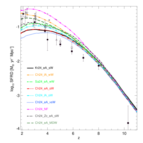
Figure 1: Evolution of the cosmic star formation rate density for all the simulations of Table 1 with box size equal to 24 Mpc/$h$. The black symbols and error bars refer to different observational estimates: Cucciati et al. (2012) - filled circles; Steidel et al. (1999) - asterisks; Ouchi et al. (2004) - plus signs; Pérez-González et al. (2005) - inverted open triangles; Schiminovich et al. (2005) - open diamonds; Bouwens et al. (2009) - open squares; Reddy & Steidel (2009) - crosses; Rodighiero et al. (2010) - open circles; van der Burg et al. (2010) - upright open triangles; Bouwens et al. (2012) - filled squares.

Since the total integrated amount of gas converted into “stars” is the same for different IMFs, the choice of IMF plays a minor role in the resulting CSFRD evolution. For example the Kr24_eA_sW (black solid line) and the Ch24_eA_sW (red triple dot-dashed line) simulations, which have exactly the same configuration aside from the IMF (Kroupa and Chabrier, respectively), are in good agreement for $z>2$.

All simulations show a similar CSFRD above redshift $z\sim 8$, but at lower redshift start to differ for different feedback implementations. Specifically, stronger feedback results in lower star formation rate density. As expected, the no-feedback simulation Ch24_NF (magenta triple dot-dashed line) shows the highest CSFRD: in this case there is no effective mechanism able to quench the star formation, and, because of the “overcooling” of gas, too many stars are formed.

Figure 1 illustrates a general trend that at higher redshift the importance of supernova driven winds increases with respect to AGN feedback. Galactic winds start to be effective at $z\leq 7$. This is visible when the Sa24_eA_wW (early AGN $+$ weak Winds, light green dot-dashed line) and the Ch24_eA_sW (early AGN $+$ strong Winds, red triple dot-dashed line) runs are compared. In these cases the main difference is related to the strength of the winds. On the other hand, the AGN feedback is particularly effective at $z\leq 5$. This can be seen by comparing the Ch24_lA_sW run (cyan triple dot-dashed line) with the Ch24_eA_sW run (red triple dot-dashed line), since the only difference is in the effectiveness of the AGN feedback. Moreover, the Ch24_lA_sW run (cyan triple dot-dashed line) falls below the Sa24_eA_wW (light green dot-dashed line), suggesting that at high redshift galactic winds regulate AGN feedback. Finally, the Ch24_eA_vsW (blue dotted line) and the Ch24_lA_wW (orange triple dot-dashed line) runs show, respectively, the lowest and the highest CSFRD among runs that include feedback.

The effect of metal cooling on the CSFRD can be evaluated by comparing the Ch24_Zc_eA_sW run (dot-dashed dark grey line) with the Ch24_eA_sW run (red triple dot-dashed line). When metal cooling is included, the star formation rate density increases at all redshifts and up to a factor of $\sim 2$ at $z=3$. This is due to the fact that in this case the gas can cool more efficiently via metal-line cooling and forms more stars with respect to gas with primordial composition.

The CSFRD for the run with momentum-driven galactic winds Ch24_eA_MDW (dark green dashed line) is in qualitative agreement with the run with late AGN feedback and weak energy-driven winds (Ch24_lA_wW, orange triple dot-dashed line). As we will discuss in the next sections, momentum-driven winds are less efficient than energy-driven winds in the most massive halos. As a result, the CSFRD of the Ch24_eA_MDW run at $z\apprle 6$ is higher than all the runs including strong energy-driven winds.

4 Star formation rate functions

4.1 Observational data

In this paper we study the evolution of the star formation rate function (SFRF) of high redshift galaxies. We compare our simulations with the observational results of Smit et al. (2012), in which the authors investigated the SFRF of galaxies in the redshift range $z\sim 4-7$. Smit et al. (2012) adopted two different methods (stepwise and analytical) to convert UV Luminosity Functions (LFs) into SFR functions. The two methods are consistent with each other and the results are well described by a set of Schechter functions (Schechter, 1976):

$$\phi({\rm SFR})\ {\rm d}\,{\rm SFR} = \phi^{\star}_{\rm SFR}\left(\frac{{\rm SFR}}{{\rm SFR}^{\star}}\right)^{\alpha_{\rm SFR}}$$ (22)

$$\times \exp\left(-\frac{{\rm SFR}}{{\rm SFR}^{\star}}\right)\frac{{\rm d}\,{\rm SFR}}{{\rm SFR}^{\star}}.$$

The analytical Schechter parameters ($\phi^{\star}_{\rm SFR}$, SFR^⋆ and $\alpha_{\rm SFR}$) of Smit et al. (2012) are shown in Table 2. We also report the stepwise determinations of the star formation rate function at $z\sim 4-7$ in Appendix A (Table 3).

We note that Salim & Lee (2012) showed that SFR functions cannot be adequately described by standard Schechter functions, but are better described by “extended” Schechter functions (where the exponential part of the standard Schechter function becomes the Sérsic function) or Saunders functions (Saunders et al., 1990). However, this does not affect the conclusions from this work.

Figure 2: Star formation rate functions at $z\sim 4-7$ for all the simulations of Table 1 with box size equal to 24 Mpc/$h$. The red filled circles with error bars and the vertical red dot-dashed lines represent the stepwise determinations of the SFR function and the observational limits of Smit et al. (2012), respectively. At each redshift, a panel showing ratios between the different simulations and the Kr24_eA_sW run (black solid line) is included. Line-styles of different simulations are as in Figure 1.

4.2 Simulated SFRFs

In Figure 2 we show the star formation rate functions at redshift $z\sim 4-7$ for all runs with box size $L=24$ Mpc/$h$, and compare these with the results of Smit et al. (2012, red filled circles with error bars). The vertical red dot-dashed lines are the observational limits in the range of SFR. At each redshift, a panel showing ratios between the different simulations and the Kr24_eA_sW run (black solid line) is included. In Appendix B we also perform box size and resolution tests using simulations with $L=18$ Mpc/$h$ and $L=12$ Mpc/$h$. These tests show that, while the simulated cosmic star formation rate density converges only at $z\sim 4.5$, the SFR in collapsed structures with mass ${\rm M}\geq 10^{9.6}$ M${}_{\rm\odot}/h$ is convergent out to $z\sim 7$. Since this mass range corresponds to galaxies above the lower limit of SFR in Smit et al. (2012), our results are robust at all redshifts considered. In this section we first discuss the simulations at different redshifts, before concentrating on individual properties of the star formation and feedback schemes.

	$\langle z\rangle$	$\phi^{\star}_{\rm SFR}\ \left(10^{-3}\ {\rm Mpc}^{-3}\right)$	$\log\frac{{\rm SFR}^{\star}}{{\rm M}_{\rm\odot}\ {\rm yr}^{-1}}$	$\alpha_{\rm SFR}$
	3.8	1.07$\pm$0.17	1.54$\pm$0.10	-1.60$\pm$0.07
	5.0	0.76$\pm$0.23	1.36$\pm$0.12	-1.50$\pm$0.12
	5.9	1.08$\pm$0.39	1.07$\pm$0.17	-1.57$\pm$0.22
	6.8	0.64$\pm$0.56	1.00$\pm$0.30	-1.96$\pm$0.35

Table 2: Parameters of the Schechter-like approximation ($\phi^{\star}_{\rm SFR}$, SFR^⋆ and $\alpha_{\rm SFR}$) to represent the star formation rate functions of galaxies at $z\sim 4-7$ from Smit et al. (2012).

At redshift $z=6.8$ (bottom right panel of Figure 2) the no-feedback run (magenta triple dot-dashed line), overproduces the number of systems in the high SFR tail ($\log\,\frac{{\rm SFR}}{{\rm M}_{\odot}\ {\rm yr}^{-1}}\apprge 0.8$) with respect to all the other simulations, due to the overcooling of gas. In this SFR range, the no-feedback run is marginally consistent with the observations. All the other runs are consistent with each other and with the observations, regardless the configuration used for strength of feedback and choice of IMF. This means that at $z\sim 7$ our simulations are not able to discriminate different schemes of feedback. The simulation with metal cooling included (Ch24_Zc_eA_sW - dark grey dot-dashed line) does show an increase of the SFRF for systems with $-0.07<\log\,\frac{{\rm SFR}}{{\rm M}_{\odot}\ {\rm yr}^{-1}}\apprle 1.0$. As stated in Section 3, this is due to the fact that when the metals are included in the cooling function, the gas can cool more efficiently and produce more stars than gas of primordial composition. As a result, there are more halos inside the observational window and an increased value of the SFRF. Inside the observational limits, the simulation with momentum-driven winds (Ch24_eA_MDW - dark green dashed line) is in agreement with all the energy-driven wind runs. However, the momentum-driven scaling of the wind mass loading factor results in a great suppression of the SFRF in low mass halos. We will discuss the difference between costant winds and momentum-driven winds in detail in Sub-section 4.2.5.

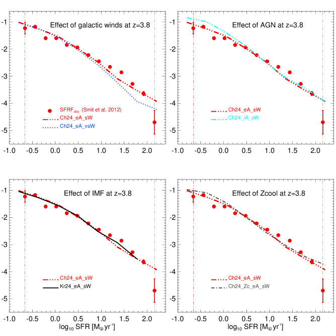
Figure 3: Star formation rate functions at redshift $z=3.8$. Top left panel: effect of galactic winds. Top right panel: effect of AGN feedback. Bottom left panel: effect of IMF. Bottom right panel: effect of metal cooling. In each panel, the red filled circles with error bars and the vertical red dot-dashed lines represent the stepwise determination of the SFR function and the observational limits of Smit et al. (2012), respectively.

A similar trend is seen at redshift $z=5.9$ (bottom left panel). Aside from the no-feedback case, we again have good agreement between observations and simulations, though the simulations slightly overproduce objects with low star formation rates.

For $z=5.0$ (top right panel) we predict more galaxies with low and medium SFRs ($\log\,\frac{{\rm SFR}}{{\rm M}_{\odot}\ {\rm yr}^{-1}}\apprle 0.5$) than observed. The effect of the different feedback mechanisms starts to become more visible at this redshift. Simulations with weak feedback (Ch24_lA_sW; Sa24_eA_wW; Ch24_lA_wW) show an excess of systems with SFR in the range $-0.33<\log\,\frac{{\rm SFR}}{{\rm M}_{\odot}\ {\rm yr}^{-1}}\apprle 0.8$, with respect to simulations with strong feedback (kr24_eA_sW; Ch24_eA_sW; Ch24_eA_vsW) and the momentum-driven wind run Ch24_eA_MDW. The simulation with metal cooling (Ch24_Zc_eA_sW) again shows an increase of the SFRF at $\log\,\frac{{\rm SFR}}{{\rm M}_{\odot}\ {\rm yr}^{-1}}\apprle 1.0$, with respect to the corresponding simulation without metal cooling (Ch24_eA_sW).

Finally, the behaviour of the different simulations becomes more clear at $z=3.8$ (top left panel). The no-feedback run overproduces systems throughout the observational window. At this redshift, it is possible to distinguish the relative impact of different feedback mechanisms. In Figure 3 we highlight the influence of different forms of feedback, metal cooling and IMF on the SFRF at $z=3.8$. We discuss these different effects in the following sub-sections.

4.2.1 Effect of feedback

To isolate the effects of feedback at $z=3.8$ we only consider those simulations which have a Chabrier IMF, energy-driven winds and no metal cooling. Among these simulations, the high SFR tail ($\log\,\frac{{\rm SFR}}{{\rm M}_{\odot}\ {\rm yr}^{-1}}\apprge 1.3$) of the run with late AGN feedback and weak winds (Ch24_lA_wW) produces the highest values of the SFRF. The second and the third highest both have strong winds but late and early AGN feedback, respectively (Ch24_lA_sW and Ch24_eA_sW). The latter two simulations do not show any difference at high SFRs (even though the implementation of the AGN feedback is different). However, they have lower SFRF than the Ch24_lA_wW model. Finally, the very strong winds case (Ch24_eA_vsW - blue dotted line) has the lowest value of the SFRF in the high SFR tail (this feature is already visible at $z=5.0$). The top left panel of Figure 3 shows the isolated effect of SN feedback by comparing Ch24_eA_sW with Ch24_eA_vsW.

The situation is different at low star formation rates ($\log\,\frac{{\rm SFR}}{{\rm M}_{\odot}\ {\rm yr}^{-1}}\apprle 0.2$). In this range, the Ch24_lA_wW run produces more systems with respect to the other three runs. However, the Ch24_lA_sW run and the Ch24_eA_sW run are not equal at these low SFRs. The SFRF of the early AGN simulation is lowered, and agrees well with the very strong winds run (Ch24_eA_vsW). This suggests that at $z=3.8$ the AGN feedback in our simulations is important in shaping the SFRF in the low SFR range. We discuss in Section 5 how this is related to our black hole seeding scheme. The effect of AGN feedback can be clearly seen in the top right panel of Figure 3.

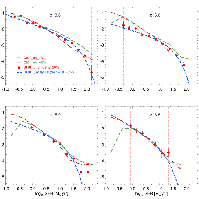
Figure 4: Star formation rate functions at $z\sim 4-7$: comparison of energy- and momentum-driven galactic winds. Red triple dot-dashed lines: Ch24_eA_sW run with Chabrier initial mass function, early AGN feedback and energy-driven galactic winds of (constant) velocity $v_{\rm w}=450$ km/s. Dark green dashed lines: Ch24_eA_MDW run with Chabrier initial mass function, early AGN feedback and momentum-driven galactic winds ($v_{\rm w}=2\times v_{\rm circ}$). The blue dot-dashed lines are the observed analytical Schechter-like SFRFs shown in Table 2. The red filled circles with error bars are the stepwise determinations of the SFRF shown in Table 3 (Appendix A). The vertical red dot-dashed lines mark the observational limits. All the observational results are from Smit et al. (2012).

4.2.2 Effect of IMF

At all redshifts, the choice of IMF has only a minor impact on the SFRF. By comparing the Ch24_eA_sW and the Kr24_eA_sW runs we see agreement at all SFRs, apart from a small deviation at the high SFR tail, where the SFRF of the Chabrier IMF falls below the SFRF of the Kroupa IMF (see bottom left panel of Figure 3). The fact that the IMF has a marginal impact is not surprising, given that it affects mostly metal production and metal-line cooling is not included in these two simulations. In principle, changing the IMF should also change the number of SN produced and, therefore, the corresponding budget of energy feedback. However, since in our kinetic feedback model we fix both wind velocity and mass upload rate, the corresponding efficiency is not related to the number of SN. In fact, this number enters only as thermal feedback to regulate star formation in the ISM effective model. Since this feedback channel is quite inefficient, the net result is that the IMF does not have a sizeable effect on the SFR.

4.2.3 Effect of metal cooling

By comparing the Ch24_Zc_eA_sW and the Ch24_eA_sW runs we are able to check the influence of metal cooling on the simulated SFRFs. At $z\geq 5$, metal cooling is responsible for the increase in the number of objects with $\log\,\frac{{\rm SFR}}{{\rm M}_{\odot}\ {\rm yr}^{-1}}\apprle 1.0$. At $z=3.8$, we can see that this increment is significant only in the low star formation rate tail of the distribution (see bottom right panel of Figure 3). At this redshift, the effect of metal cooling is less important than the effect of different feedback prescriptions.

4.2.4 Relative importance of galactic winds and AGN feedback

Since the choice of IMF plays a minor role on the SFRF, we next compare the Sa24_eA_wW (Salpeter IMF) with the Ch24_lA_wW and the Ch24_lA_sW runs (Chabrier IMFs), in the top left panel of Figure 2. At high SFRs the Sa24_eA_wW and the Ch24_lA_wW are in agreement. These simulations have the same wind strength but different AGN implementations. The Ch24_lA_sW has lower SFRF than the two weak wind models. At low SFRs, the SFRF values are ranked according to: ${\rm SFRF}_{\textit{Ch24\_lA\_wW}}>{\rm SFRF}_{\textit{Ch24\_lA\_sW}}>{\rm SFRF}_{\textit{Sa24\_eA\_wW}}$. This suggests that, in our simulations at high redshift, galactic winds shape the SFRF over the whole range of star formation rates and their effect is more important than AGN feedback for halos with mass M $\apprle 10^{12}$ M_⊙/$h$ (i.e. the mass of the most massive halo at $z=3.8$). As a result of our black hole seeding scheme, the effect of AGN feedback is most visible at low SFRs (see the discussion in Section 5).

4.2.5 Constant vs. momentum-driven galactic winds

In Figure 4 we compare the evolution of the SFRF for the Ch24_eA_sW run (Chabrier IMF, early AGN feedback and energy-driven galactic winds of constant velocity $v_{\rm w}=450$ km/s - red triple dot-dashed lines) and the Ch24_eA_MDW run (Chabrier IMF, early AGN feedback and momentum-driven galactic winds - dark green dashed lines). In the figure, besides the stepwise determinations of the SFRF from Smit et al. (2012, red filled circles with error bars), we show the analytical Schechter-like SFRFs from the same work (blue dot-dashed lines; the parameters of these analytical functions are presented in Table 2). The vertical red dot-dashed lines mark the observational limits.

At $z=6.8$ the two simulations are in good agreement inside the observational window. At $z=5.9$ a slight excess of systems at $\log\,\frac{{\rm SFR}}{{\rm M}_{\odot}\ {\rm yr}^{-1}}\apprge 1.0$ is visible for the momentum-driven wind run. Moreover, as we pointed out in Section 4.2, the momentum-driven scaling of the wind mass loading factor results in a great suppression of the SFRF in low mass halos (although outside the observational limits). At lower redshift, as the mass function moves towards larger masses, this suppression becomes less pronounced and almost disappears at $z=3.8$.

At $z=5.0$ (3.8) the Ch24_eA_sW and the Ch24_eA_MDW runs produce the same SFRF for $\log\,\frac{{\rm SFR}}{{\rm M}_{\odot}\ {\rm yr}^{-1}}\apprle 0.8$ ($\log\,\frac{{\rm SFR}}{{\rm M}_{\odot}\ {\rm yr}^{-1}}\apprle 0.5$). However, in massive halos momentum-driven winds are less efficient than energy-driven winds in quenching the star formation rate. Consequently, in the high end of the distribution ${\rm SFRF}_{\textit{Ch24\_eA\_MDW}}>{\rm SFRF}_{\textit{Ch24\_eA\_sW}}$. It is straightforward to understand this trend for the Ch24_eA_MDW simulation. In small halos the velocity of the winds is low, but their efficiency is large ($\eta\propto v_{\rm w}^{-1}$). Therefore, even low velocity winds are efficient in stopping the ongoing star formation rate. On the other hand, in massive halos winds have velocities $v_{\rm w}\gg 450$ km/s and small loading factors ($\eta\ll 2$). For this reason, only a few wind particles are created and these are not sufficient to effectively suppress the formation of stars (even if they can easily escape from galaxies and reach the IGM). Overall, the momentum-driven wind simulation is consistent with the observations of Smit et al. (2012).

For further comparison, we performed several tests by changing the velocity of the winds ($v_{\rm w}=v_{\rm circ}$ instead of $v_{\rm w}=2\times v_{\rm circ}$: run Ch24_eA_MDW_DVS, where DVS stands for “Different Velocity Scaling”), and also using the energy-driven scaling of the wind mass loading factor adopted by Puchwein & Springel (2013): $\eta\propto v_{\rm w}^{-2}$ (run Ch24_eA_EDW). The result of these tests is shown in Figure 5. Our conclusion is that in order to reproduce the SFRFs at high redshift, a non-aggressive variable wind scaling is needed, otherwise the number of objects with low SFRs is greatly suppressed, while at the same time winds are not effective in the most massive systems. As a consequence, the SFRFs from the Ch24_eA_MDW run are in a qualitative agreement with the constant wind models used in this work.

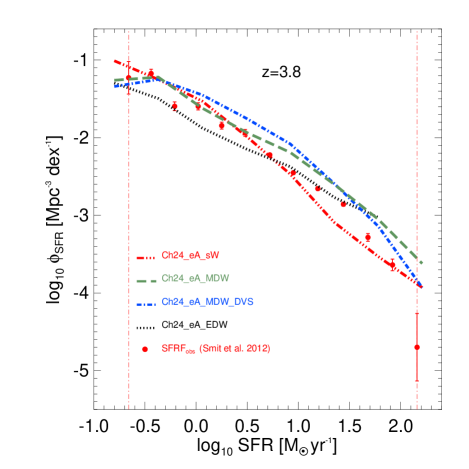
Figure 5: Star formation rate function at $z=3.8$: comparison of different choices of parameters for the energy- and momentum-driven galactic winds. All the simulations shown have a Chabrier initial mass function and early AGN feedback. Red triple dot-dashed line: Ch24_eA_sW run with energy-driven galactic winds of constant velocity $v_{\rm w}=450$ km/s and loading factor $\eta=2$. Dark green dashed line: Ch24_eA_MDW run with momentum-driven winds ($v_{\rm w}=2\times v_{\rm circ}$ and $\eta=2\times\frac{450\,\,{\rm km/s}}{v_{\rm w}}$). Blue dot-dashed line: Ch24_eA_MDW_DVS run with momentum-driven winds and different velocity scaling ($v_{\rm w}=v_{\rm circ}$ and $\eta=2\times\frac{450\,\,{\rm km/s}}{v_{\rm w}}$). Black dotted line: Ch24_eA_EDW run with energy-driven winds ($v_{\rm w}=2\times v_{\rm circ}$ and $\eta=2\times\left(\frac{450\,\,{\rm km/s}}{v_{\rm w}}\right)^{2}$). The last two simulations have been run only as a comparison and are not part of the set discussed throughout this paper. The red filled circles with error bars and the vertical red dot-dashed lines represent, respectively, the stepwise determination of the SFR function and the observational limits of Smit et al. (2012) at $z=3.8$.

Figure 6: Star formation rate functions at $z\sim 4-7$ for our best model with Kroupa initial mass function, early AGN feedback and strong energy-driven galactic winds of velocity $v_{\rm w}=450$ km/s (black solid lines). The black error bars are the Poissonian uncertainties of the simulated SFRFs. The blue dot-dashed lines are the observed analytical Schechter-like SFRFs shown in Table 2. The red filled circles with error bars are the stepwise determinations of the SFRF shown in Table 3 (Appendix A). The vertical red dot-dashed lines mark the observational limits. All the observational results are from Smit et al. (2012).

4.2.6 Best model

In Figure 6 we show the star formation rate functions at redshift $z\sim 4-7$ for our best model: Kr24_eA_sW (Kroupa IMF, early AGN feedback and strong energy-driven galactic winds with $v_{\rm w}=450$ km/s). This simulation provides the best description of the observations among the models considered in our analysis, especially at $z=3.8$. However, like all the other runs that include feedback, at $z=5.0$ it overproduces objects with $\log\,\frac{{\rm SFR}}{{\rm M}_{\odot}\ {\rm yr}^{-1}}\apprle 0.5$. This either suggests a bias in the observations, or that the calibration of galactic winds and AGN feedback must be varied in order to reproduce the observational data over the redshift range $4\leq z\leq 7$.

In Figure 6, the blue dot-dashed lines and the red filled circles with error bars are, respectively, the analytical Schechter-like SFRFs and the stepwise determinations of the SFRF of Smit et al. (2012). The vertical red dot-dashed lines mark the observational limits. We also include the Poissonian uncertainties for the simulated SFRFs (black error bars), in order to provide an estimate of the errors from our finite box size. The uncertainties are larger at high SFRs due to the small number of massive halos in the box.

5 Discussion

At the highest redshift considered in this work, we find that our simulations are not able to distinguish the effect of different feedback prescriptions. In fact, at $z\sim 7$ all runs with feedback included reproduce the observational data. On the other hand, the case with no feedback fails to fit the observations. An important conclusion is therefore that feedback effects start to be important from very high redshift. Moving to lower redshift (and especially at $z=3.8$), different feedback configurations show different trends, implying that the SFRF can be used to probe the physics of star formation and feedback at high $z$. As discussed in Section 3, supernova driven galactic winds start to be effective at $z\leq 7$.

In the top left panel of Figure 3 the Ch24_eA_sW run and the Ch24_eA_vsW run are compared at $z=3.8$. They have exactly the same configuration except for the wind velocity (450 km/s and 550 km/s, respectively). The two SFRFs are in agreement for $\log\,\frac{{\rm SFR}}{{\rm M}_{\odot}\ {\rm yr}^{-1}}\apprle 1.0$, while in the high SFR tail ${\rm SFRF}_{\textit{Ch24\_eA\_sW}}>{\rm SFRF}_{\textit{Ch24\_eA\_vsW}}$. This indicates that, for halos with $\log\,\frac{{\rm SFR}}{{\rm M}_{\odot}\ {\rm yr}^{-1}}\apprle 1.0$, the effect of the two wind configurations is the same: both efficiently remove gas particles from the central regions and kick them out of the collapsed structures. At higher SFRs/masses, weaker winds become less effective in expelling gas and wind particles remain trapped within halos. We stress that in our energy-driven scheme, even if we consider different wind velocities, the efficiency of the winds is fixed to $\eta=\dot{\rm M}_{\rm w}/\dot{\rm M}_{\star}=2$ (see Eq. 13). As a consequence, for different configurations the wind mass loading ($\dot{\rm M}_{\rm w}$) is the same at a given star formation rate ($\dot{\rm M}_{\star}$). Since we also decouple wind particles from the hydrodynamics for a certain period of time, ejecta at higher velocities are more effective in removing gas from halos. This in turn explains why ${\rm SFRF}_{\textit{Ch24\_eA\_sW}}>{\rm SFRF}_{\textit{Ch24\_eA\_vsW}}$ in the high SFR tail of the distribution.

We compared the constant galactic wind models with a momentum-driven variable wind scheme. In this model, the velocity of the wind depends on the circular velocity of the halo $v_{\rm w}=2\times v_{\rm circ}$. The mass loading factor $\eta=2\times\frac{450\,\,{\rm km/s}}{v_{\rm w}}$ ($\eta=2$ if the wind velocity is equal to our reference constant “strong” wind model $v_{\rm w}=450$ km/s). Overall, the momentum-driven wind simulation is in agreement with the constant wind models and consistent with the observations of Smit et al. (2012).

While at redshift $z\geq 3.8$ galactic winds are already in place and dominate the feedback mechanisms, AGN feedback is not yet very efficient. In our AGN model, we seed all the halos above a given mass threshold (M_th) with a central SMBH of mass M_seed, provided they contain a minimum mass fraction in stars $f_{\star}$ (see the end of Sub-section 2.3.3). These SMBHs can then grow via gas accretion and through mergers with other SMBHs. Our simulations explored two regimes for the AGN feedback, with varied M_th, $f_{\star}$, M_seed and the maximum accretion radius $R_{\rm ac}$. In the “early AGN” configuration we reduced M_th, $f_{\star}$ and M_seed and increased $R_{\rm ac}$, with respect to the “late AGN” configuration. However, the radiative efficiency ($\epsilon_{\rm r}$) and the feedback efficiency ($\epsilon_{\rm f}$) are the same in the two regimes. Decreasing the threshold mass for seeding a SMBH increases the effect of AGN feedback on halos with low SFRs by construction, since we allow the presence of a black hole in lower mass halos (compare the Ch24_eA_sW run and the Ch24_lA_sW run in the upper right panel of Figure 3). The case with early AGN leads asymptotically to the Magorrian relation (Magorrian et al., 1998) at low redshift, but imposes high black hole$/$halo mass ratios in small galaxies at early times. As a result, ${\rm SFRF}_{\textit{Ch24\_eA\_sW}}<{\rm SFRF}_{\textit{Ch24\_lA\_sW}}$ in the low SFR tail of the distribution. On the other hand, there is no difference between the Ch24_eA_sW run and the Ch24_lA_sW run at high SFRs. At $z=3.8$, halos with $\log\,\frac{{\rm SFR}}{{\rm M}_{\odot}\ {\rm yr}^{-1}}\geq 1.0$ have stellar masses $10^{10}$ M_⊙/$h\leq$ M${}_{\star}\leq 10^{11}$ M_⊙/$h$. For these halos, the central SMBHs have grown to masses $5\times 10^{7}$ M${}_{\rm\odot}/h\leq$ M${}_{\rm SMBH}\leq 5\times 10^{8}$ M_⊙/$h$ and are accreting at a moderate level. As shown in Di Matteo et al. (2005), in these objects the star formation rate is essentially unaffected by the presence of the black holes, since the SMBHs have not yet reached a regime of self-regulating growth. Due to the small box size, at high redshift our simulations are not able to form cluster-sized objects with total mass M $\apprge 10^{12}$ M_⊙/$h$, where the black hole growth is expected to be exponential at early times (Di Matteo et al., 2008). In this case, the central SMBHs would grow until they release sufficient energy to generate outflows and prevent further star formation. This explains why we do not see any AGN feedback effect in the high star formation rate tail of the SFRF.

In conclusion, in our simulations the interplay between galactic winds and AGN feedback suggests that at high redshift SN driven winds are essential to reproduce the observed SFRFs. According to our scheme, the effect of AGN feedback in the low end of the luminosity/SFR functions is sensitive to the seeding of super-massive black holes. We are extending this work to lower redshift, in order to compare our results with different observations and other theoretical works. For example, Davé et al. (2011) examined the growth of the stellar content of galaxies at $z=0-3$. They ran four different galactic wind models. With these simulations, they produced stellar mass and star formation rate functions to quantify the effects of outflows on the galactic evolution at low redshift. In their simulations, winds are responsible for the shape of the faint end slope of the SFR function at $z=0$ (top left panel of Figure 2 in Davé et al., 2011). AGN feedback is not included and, as a result, their simulations overproduce the number of objects in the high star formation rate tail. We will show how in our simulations AGN are crucial to reproduce the observed high end of the luminosity/SFR functions at low redshift ($z\apprle 1$), as pointed out by other authors (Puchwein & Springel, 2013) and also by semi-analytic models (e.g. Croton et al., 2006; Bower et al., 2006).

6 Conclusions

In this paper we have presented a new set of cosmological simulations, Angus (AustraliaN GADGET-3 early Universe Simulations), run with the hydrodynamic code P-GADGET3(XXL). We have used these to investigate the star formation rate function of high redshift galaxies ($z\sim 4-7$), with comparison to the observations of Smit et al. (2012). In particular, we have focused on the role of feedback from SN and AGN and studied the impact of metal cooling and different IMFs. We ran 11 simulations with various feedback configurations and box sizes ($L=24$, 18 and 12 Mpc/$h$). We used the Springel & Hernquist (2003) implementation of SN energy-driven galactic winds. In particular, we explored three different configurations: weak, strong and very strong winds of constant velocity $v_{\rm w}=350$, 450 and 550 km/s, respectively. Moreover, following Puchwein & Springel (2013), in one simulation we adopted variable momentum-driven galactic winds. We also explored two regimes for the AGN feedback (early and late). The early AGN scheme imposes high black hole$/$halo mass ratios in small galaxies at early times. This configuration leads asymptotically to the Magorrian relation (Magorrian et al., 1998) at low redshift, but accentuates the effect of AGN in low SFR/mass halos at high $z$. We considered three different IMFs (Salpeter, 1955; Kroupa et al., 1993; Chabrier, 2003) and the effect of metal cooling (see Section 2.4). We have performed box size and resolution tests to check the convergence of the results from our simulations (Appendix B). Overall, these tests confirm that the SFR in collapsed structures with mass ${\rm M}\geq 10^{9.6}$ M${}_{\rm\odot}/h$ is convergent at all the redshifts considered.

The main results and conclusions of this work can be summarised as follows:

• We studied the evolution of the cosmic star formation rate density (CSFRD). Galactic winds start to be effective at $z\leq 7$, while the AGN feedback becomes important later on, at $z\leq 5$. When metal cooling is included, the cosmic star formation rate density increases at all redshifts and up to a factor of $\sim 2$ at $z=3$. On the other hand, in our simulations the choice of IMF plays a minor role on the CSFRD evolution.

• We explored the star formation rate functions (SFRFs) of galaxies at redshift $z\sim 4-7$. At $z=6.8$, our simulations are not able to discriminate different feedback prescriptions and all runs that include feedback reproduce the observational results of Smit et al. (2012). However, the no-feedback simulation fails to fit the observations, indicating that feedback effects start to be important and need to be taken into account from very high redshift. The key factor required to reproduce the observed SFRFs at lower redshift, is a combination of strong winds and early AGN feedback.

• In our simulations, supernova driven galactic winds shape the SFRF in the whole range of star formation rates. This conclusion is not qualitatively dependent on the model for AGN feedback.

• At all the redshifts considered, the choice of IMF has a minor impact on the SFRFs. On the other hand, metal cooling is responsible for the increase in the number of objects with low and intermediate star formation rates. However, at $z\sim 4$ the effect of metal cooling is less important than the effect of different feedback prescriptions.

• To reproduce the SFRFs at $z\apprge 4$, a non-aggressive variable wind scaling is needed, otherwise the amount of objects with low SFRs is greatly suppressed and at the same time winds are not effective in the most massive systems. As a result, the SFRFs from our momentum-driven wind simulation are in a qualitative agreement with the constant (energy-driven) wind models used in this work.

We are exploring the interplay between galactic winds and AGN feedback at high redshift in a companion paper (Katsianis et al., 2013). In that work we analyse the stellar mass functions and the star formation rate$-$stellar mass relations for the sample of galaxies considered in this work. We are also planning to explore more feedback configurations and in particular different parameters for the AGN feedback and the new wind models of Barai et al. (2013).

	$\log\,\frac{{\rm SFR}}{{\rm M}_{\odot}\ {\rm yr}^{-1}}$		$\phi_{\rm SFR}\ \left({\rm Mpc}^{-3}\ {\rm dex}^{-1}\right)$
		$z\sim 4$
	-0.66		0.05920$\pm$0.02855
	-0.44		0.06703$\pm$0.00838
	-0.21		0.02537$\pm$0.00326
	0.02		0.02534$\pm$0.00268
	0.25		0.01430$\pm$0.00144
	0.48		0.01153$\pm$0.00117
	0.72		0.00601$\pm$0.00025
	0.95		0.00354$\pm$0.00017
	1.19		0.00221$\pm$0.00012
	1.44		0.00139$\pm$0.00008
	1.68		0.00052$\pm$0.00006
	1.92		0.00023$\pm$0.00004
	2.16		0.00002$\pm$0.00002
		$z\sim 5$
	-0.33		0.01766$\pm$0.00858
	-0.11		0.01161$\pm$0.00294
	0.12		0.01076$\pm$0.00121
	0.36		0.00420$\pm$0.00046
	0.61		0.00362$\pm$0.00040
	0.86		0.00224$\pm$0.00014
	1.11		0.00121$\pm$0.00008
	1.37		0.00060$\pm$0.00006
	1.63		0.00023$\pm$0.00002
	1.89		0.00006$\pm$0.00002
		$z\sim 6$
	-0.04		0.01197$\pm$0.00262
	0.41		0.00426$\pm$0.00089
	0.77		0.00173$\pm$0.00037
	1.01		0.00110$\pm$0.00024
	1.26		0.00026$\pm$0.00008
	1.51		0.00014$\pm$0.00004
	1.77		0.00002$\pm$0.00002
	2.03		0.00002$\pm$0.00002
		$z\sim 7$
	-0.07		0.01543$\pm$0.00473
	0.15		0.00761$\pm$0.00215
	0.38		0.00513$\pm$0.00149
	0.61		0.00224$\pm$0.00075
	0.84		0.00106$\pm$0.00044
	1.08		0.00031$\pm$0.00019
	1.32		0.00033$\pm$0.00018

Table 3: Stepwise determinations of the SFR function at $z\sim 4-7$ (Smit et al., 2012).

Appendix A: Observed stepwise SFRFs

Table 3 shows the Smit et al. (2012) stepwise determinations of the star formation rate function $\phi_{\rm SFR}$ from dust-corrected UV luminosity functions at $z\sim 4-7$.

Appendix B: Box size and resolution tests

In this appendix we perform box sixe and resolution tests, in order to check the convergence of the results from our simulations. We underline that in this paper the smaller the box size of a run, the higher its mass/spatial resolution. However, the box size sets an upper limit on the mass of the halos that can be formed in the simulated volume. Therefore, higher resolution means poorer statistics at the high mass end of the halo mass function.

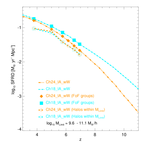
Figure 7: Evolution of the cosmic star formation rate density: box size and resolution tests. Top panel: we compare $a)$ the Chabrier IMF, Early AGN, Strong Winds configuration for two different box sizes: $L=24$ Mpc/$h$ (Ch24_eA_sW - red triple dot-dashed line) and $L=12$ Mpc/$h$ (Ch12_eA_sW - black dotted line) and $b)$ the Chabrier IMF, Late AGN, Weak Winds configuration for $L=24$ Mpc/$h$ (Ch24_lA_wW - orange triple dot-dashed line) and $L=18$ Mpc/$h$ (Ch18_lA_wW - cyan dot-dashed line). Bottom left panel: the dotted black line represents the Ch12_eA_sW run and the red triple dot-dashed line represents the Ch24_eA_sW run, as in the top panel. At any given redshift, the filled black squares and red diamonds mark the total SFR density in collapsed structures. The open black squares and red diamonds show the SFR density in halos of mass $10^{9.6}$ M${}_{\rm\odot}/h\leq{\rm M}\leq 10^{10.7}$ M${}_{\rm\odot}/h$. Bottom right panel: same as the bottom left panel for runs Ch18_lA_wW (cyan dot-dashed line) and Ch24_lA_wW (orange triple dot-dashed line). The open cyan squares and orange diamonds show the SFR density in halos of mass $10^{9.6}$ M${}_{\rm\odot}/h\leq{\rm M}\leq 10^{11.1}$ M${}_{\rm\odot}/h$.

In Figure 7 we compare the evolution of the cosmic star formation rate density for runs with box size equal to $L=24$ Mpc/$h$, $L=18$ Mpc/$h$ and $L=12$ Mpc/$h$. In the top panel, four simulations are considered: two in the late AGN $+$ weak Winds scenario (Ch24_lA_wW - orange triple dot-dashed line and Ch18_lA_wW - cyan dot-dashed line) and two in the early AGN $+$ strong Winds scenario (Ch24_eA_sW - red triple dot-dashed line and Ch12_eA_sW - black dotted line). We see from the plot that runs with the same configuration converge at redshift $z\sim 4.5$. Moreover, the two simulations with higher resolutions (Ch12 and Ch18) show a higher star formation rate density with respect to the other two runs because they can resolve higher densities at earlier times.

In the bottom left panel the red triple dot-dashed and black dotted lines refer, respectively, to the Ch24_eA_sW and the Ch12_eA_sW runs already shown in the top panel. The filled black squares and red diamonds mark the cosmic SFR density in collapsed FoF halos, at $4\leq z\leq 7$. The plot shows that all the star formation occurs inside halos, as we expect. Most importantly, the open black squares and red diamonds mark the SFR in halos of mass $10^{9.6}$ M${}_{\rm\odot}/h\leq{\rm M}\leq 10^{10.7}$ M${}_{\rm\odot}/h$. The lower limit corresponds to the mass of a halo resolved with 100 DM particles in the Ch24 simulation (the run with lower resolution). This is our mass confidence limit. The upper limit is the mass of the most massive halo in the Ch12 simulation (the run with smaller box size). In this mass range the two simulations converge at all the redshifts considered in this work. We define this mass interval as the “overlapping mass range”.

In the bottom right panel, we compare the Ch24_lA_wW (orange triple dot-dashed line) and the Ch18_lA_wW (cyan dot-dashed line) runs. The results of this panel are consistent with the results shown in the bottom left panel. In this case, the open cyan squares and orange diamonds mark the SFR in halos of mass $10^{9.6}$ M${}_{\rm\odot}/h\leq{\rm M}\leq 10^{11.1}$ M${}_{\rm\odot}/h$. The upper limit is now higher than before, corresponding to the larger box size of the Ch18 with respect to the Ch12. In this mass range the two simulations converge at all the redshifts considered. This demonstrates that, even if the total SFR in the different boxes does not converge untill $z\sim 4.5$, the SFR in collapsed structures with mass in the overlapping mass range has converged at much earlier times.

In Figure 8 we show the box size and resolution tests for the star formation rate functions at $z\sim 4-7$. We compare the same simulations used above: Ch24_eA_sW (red triple dot-dashed line), Ch12_eA_sW (black dotted line), Ch24_lA_wW (orange triple dot-dashed line) and Ch18_lA_wW (cyan dot-dashed line). Overplotted are the data (red filled circles with error bars) and the observational limits (vertical red dot-dashed lines) of Smit et al. (2012). At all redshifts considered, the Ch12 run shows poorer statistics at high SFR with respect to the other runs. This is due to its smaller box size, since there is a positive SFR$-$halo mass correlation and the box size sets an upper limit on the mass of the halos in the simulation. At redshift $z\leq 5$ ($5<z\leq 7$) the Ch12 run converges with the corresponding Ch24_eA_sW run in the range $\log\,\frac{{\rm SFR}}{{\rm M}_{\odot}\ {\rm yr}^{-1}}\apprle 0.5$ ($\log\,\frac{{\rm SFR}}{{\rm M}_{\odot}\ {\rm yr}^{-1}}\apprle 0.2$). On the other hand, inside the observational windows of Smit et al. (2012) the Ch18 run agrees well with the corresponding Ch24_lA_wW at all redshifts. A small difference is visible at $z=3.8$ for $\log\,\frac{{\rm SFR}}{{\rm M}_{\odot}\ {\rm yr}^{-1}}\apprle-0.3$. This is due to the fact that in this SFR range the resolution limit of the Ch24 simulations is reached. In fact, the Ch24_eA_sW and the Ch24_lA_wW have the same SFRF value in the first SFR bin (at all the redshifts considered), even if their configurations are quite different. This feature is also visible in Figure 2 where the various Ch24 runs are compared.

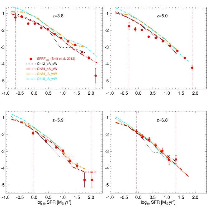
Figure 8: Star formation rate functions at $z\sim 4-7$: box size and resolution tests. At each redshift, the red filled circles with error bars and the vertical red dot-dashed lines represent the stepwise determinations of the SFR function and the observational limits of Smit et al. (2012), respectively. Line-styles of different simulations are as in Figure 7.

To summarise, all the box size and resolution tests presented above show that, even if the cosmic SFR density converges at $z\sim 4.5$, our results are robust at $z\leq 7$, provided only halos of mass ${\rm M}\geq 10^{9.6}$ M${}_{\rm\odot}/h$ are taken into account.

References

- Barai et al. (2013) Barai P., Viel M., Borgani S., Tescari E., Tornatore L., Dolag K., Killedar M., Monaco P., D’Odorico V., Cristiani S., 2013, MNRAS, 430, 3213
- Bernardi et al. (2010) Bernardi M., Shankar F., Hyde J. B., Mei S., Marulli F., Sheth R. K., 2010, MNRAS, 404, 2087
- Bondi (1952) Bondi H., 1952, MNRAS, 112, 195
- Booth & Schaye (2009) Booth C. M., Schaye J., 2009, MNRAS, 398, 53
- Bouwens et al. (2009) Bouwens R. J., Illingworth G. D., Franx M., Chary R.-R., Meurer G. R., Conselice C. J., Ford H., Giavalisco M., van Dokkum P., 2009, ApJ, 705, 936
- Bouwens et al. (2007) Bouwens R. J., Illingworth G. D., Franx M., Ford H., 2007, ApJ, 670, 928
- Bouwens et al. (2012) Bouwens R. J., Illingworth G. D., Oesch P. A., Franx M., Labbé I., Trenti M., van Dokkum P., Carollo C. M., González V., Smit R., Magee D., 2012, ApJ, 754, 83
- Bouwens et al. (2011) Bouwens R. J., Illingworth G. D., Oesch P. A., Labbé I., Trenti M., van Dokkum P., Franx M., Stiavelli M., Carollo C. M., Magee D., Gonzalez V., 2011, ApJ, 737, 90
- Bower et al. (2006) Bower R. G., Benson A. J., Malbon R., Helly J. C., Frenk C. S., Baugh C. M., Cole S., Lacey C. G., 2006, MNRAS, 370, 645
- Chabrier (2003) Chabrier G., 2003, PASP, 115, 763
- Choi & Nagamine (2012) Choi J.-H., Nagamine K., 2012, MNRAS, 419, 1280
- Croton et al. (2006) Croton D. J., Springel V., White S. D. M., De Lucia G., Frenk C. S., Gao L., Jenkins A., Kauffmann G., Navarro J. F., Yoshida N., 2006, MNRAS, 367, 864
- Cucciati et al. (2012) Cucciati O., et al., 2012, A&A, 539, A31
- Davé et al. (2011) Davé R., Oppenheimer B. D., Finlator K., 2011, MNRAS, 415, 11
- Di Matteo et al. (2008) Di Matteo T., Colberg J., Springel V., Hernquist L., Sijacki D., 2008, ApJ, 676, 33
- Di Matteo et al. (2005) Di Matteo T., Springel V., Hernquist L., 2005, Nat, 433, 604
- Dolag et al. (2009) Dolag K., Borgani S., Murante G., Springel V., 2009, MNRAS, 399, 497
- Dolag et al. (2004) Dolag K., Jubelgas M., Springel V., Borgani S., Rasia E., 2004, ApJ, 606, L97
- Dolag & Stasyszyn (2009) Dolag K., Stasyszyn F., 2009, MNRAS, 398, 1678
- Dolag et al. (2005) Dolag K., Vazza F., Brunetti G., Tormen G., 2005, MNRAS, 364, 753
- Fabjan et al. (2010) Fabjan D., Borgani S., Tornatore L., Saro A., Murante G., Dolag K., 2010, MNRAS, 401, 1670
- Ferland et al. (2013) Ferland G. J., Porter R. L., van Hoof P. A. M., Williams R. J. R., Abel N. P., Lykins M. L., Shaw G., Henney W. J., Stancil P. C., 2013, ArXiv e-print: 1302.4485
- Finlator et al. (2011) Finlator K., Oppenheimer B. D., Davé R., 2011, MNRAS, 410, 1703
- Fontanot et al. (2012) Fontanot F., Cristiani S., Santini P., Fontana A., Grazian A., Somerville R. S., 2012, MNRAS, 421, 241
- González et al. (2011) González V., Labbé I., Bouwens R. J., Illingworth G., Franx M., Kriek M., 2011, ApJ, 735, L34
- Guo et al. (2011) Guo Q., White S., Boylan-Kolchin M., De Lucia G., Kauffmann G., Lemson G., Li C., Springel V., Weinmann S., 2011, MNRAS, 413, 101
- Haardt & Madau (2001) Haardt F., Madau P., 2001, in Neumann D. M., Tran J. T. V., eds, Clusters of Galaxies and the High Redshift Universe Observed in X-rays Modelling the UV/X-ray cosmic background with CUBA
- Hopkins (2004) Hopkins A. M., 2004, ApJ, 615, 209
- Hopkins (2013) Hopkins P. F., 2013, MNRAS, 428, 2840
- Iannuzzi & Dolag (2011) Iannuzzi F., Dolag K., 2011, MNRAS, 417, 2846
- Jaacks et al. (2012) Jaacks J., Choi J.-H., Nagamine K., Thompson R., Varghese S., 2012, MNRAS, 420, 1606
- Kannan et al. (2013) Kannan R., Stinson G. S., Macciò A. V., Brook C., Weinmann S. M., Wadsley J., Couchman H. M. P., 2013, ArXiv e-print: 1302.2618
- Katsianis et al. (2013) Katsianis A., Tescari E., Wyithe S., 2013, ArXiv e-print: 1312.4964
- Kennicutt (1998) Kennicutt Jr. R. C., 1998, ApJ, 498, 541
- Kereš et al. (2012) Kereš D., Vogelsberger M., Sijacki D., Springel V., Hernquist L., 2012, MNRAS, 425, 2027
- Komatsu et al. (2011) Komatsu E., et al., 2011, ApJS, 192, 18
- Kroupa et al. (1993) Kroupa P., Tout C. A., Gilmore G., 1993, MNRAS, 262, 545
- Lee et al. (2012) Lee K.-S., Ferguson H. C., Wiklind T., Dahlen T., Dickinson M. E., Giavalisco M., Grogin N., Papovich C., Messias H., Guo Y., Lin L., 2012, APG, 752, 66
- Magorrian et al. (1998) Magorrian J., Tremaine S., Richstone D., Bender R., Bower G., Dressler A., Faber S. M., Gebhardt K., Green R., Grillmair C., Kormendy J., Lauer T., 1998, AJ, 115, 2285
- Maio et al. (2007) Maio U., Dolag K., Ciardi B., Tornatore L., 2007, MNRAS, 379, 963
- Maio et al. (2013) Maio U., Dotti M., Petkova M., Perego A., Volonteri M., 2013, ApJ, 767, 37
- Maio et al. (2011) Maio U., Khochfar S., Johnson J. L., Ciardi B., 2011, MNRAS, 414, 1145
- Martin (1999) Martin C. L., 1999, ApJ, 513, 156
- Martin (2005) Martin C. L., 2005, ApJ, 621, 227
- Murante et al. (2011) Murante G., Borgani S., Brunino R., Cha S.-H., 2011, MNRAS, 417, 136
- Nelson et al. (2013) Nelson D., Vogelsberger M., Genel S., Sijacki D., Kereš D., Springel V., Hernquist L., 2013, MNRAS, 429, 3353
- Ouchi et al. (2004) Ouchi M., Shimasaku K., Okamura S., Furusawa H., Kashikawa N., Ota K., Doi M., Hamabe M., Kimura M., Komiyama Y., Miyazaki M., Miyazaki S., Nakata F., Sekiguchi M., Yagi M., Yasuda N., 2004, ApJ, 611, 660
- Padovani & Matteucci (1993) Padovani P., Matteucci F., 1993, ApJ, 416, 26
- Percival et al. (2010) Percival W. J., et al., 2010, MNRAS, 401, 2148
- Pérez-González et al. (2005) Pérez-González P. G., Rieke G. H., Egami E., Alonso-Herrero A., Dole H., Papovich C., Blaylock M., Jones J., Rieke M., Rigby J., Barmby P., Fazio G. G., Huang J., Martin C., 2005, ApJ, 630, 82
- Planck Collaboration (2013) Planck Collaboration Ade P. A. R., Aghanim N., Armitage-Caplan C., Arnaud M., Ashdown M., Atrio-Barandela F., Aumont J., Baccigalupi C., Banday A. J., et al. 2013, ArXiv e-print: 1303.5076
- Planelles et al. (2012) Planelles S., Borgani S., Dolag K., Ettori S., Fabjan D., Murante G., Tornatore L., 2012, ArXiv e-print: 1209.5058
- Puchwein & Springel (2013) Puchwein E., Springel V., 2013, MNRAS, 428, 2966
- Read & Hayfield (2012) Read J. I., Hayfield T., 2012, MNRAS, 422, 3037
- Reddy & Steidel (2009) Reddy N. A., Steidel C. C., 2009, ApJ, 692, 778
- Riess et al. (2009) Riess A. G., Macri L., Casertano S., Sosey M., Lampeitl H., Ferguson H. C., Filippenko A. V., Jha S. W., Li W., Chornock R., Sarkar D., 2009, ApJ, 699, 539
- Rodighiero et al. (2010) Rodighiero G., et al., 2010, A&A, 515, A8
- Salim & Lee (2012) Salim S., Lee J. C., 2012, ApJ, 758, 134
- Salpeter (1955) Salpeter E. E., 1955, ApJ, 121, 161
- Santini et al. (2012) Santini P., Fontana A., Grazian A., Salimbeni S., Fontanot F., Paris D., Boutsia K., Castellano M., Fiore F., Gallozzi S., Giallongo E., Koekemoer A. M., Menci N., Pentericci L., Somerville R. S., 2012, A&A, 538, A33
- Saunders et al. (1990) Saunders W., Rowan-Robinson M., Lawrence A., Efstathiou G., Kaiser N., Ellis R. S., Frenk C. S., 1990, MNRAS, 242, 318
- Schaye et al. (2010) Schaye J., Dalla Vecchia C., Booth C. M., Wiersma R. P. C., Theuns T., Haas M. R., Bertone S., Duffy A. R., McCarthy I. G., van de Voort F., 2010, MNRAS, 402, 1536
- Schechter (1976) Schechter P., 1976, ApJ, 203, 297
- Schenker et al. (2012) Schenker M. A., Robertson B. E., Ellis R. S., Ono Y., McLure R. J., Dunlop J. S., Koekemoer A., Bowler R. A. A., Ouchi M., Curtis-Lake E., Rogers A. B., Schneider E., Charlot S., Stark D. P., Furlanetto S. R., Cirasuolo M., 2012, ArXiv e-print: 1212.4819
- Schiminovich et al. (2005) Schiminovich D., et al., 2005, ApJ, 619, L47
- Shakura & Sunyaev (1973) Shakura N. I., Sunyaev R. A., 1973, A&A, 24, 337
- Sijacki et al. (2007) Sijacki D., Springel V., Di Matteo T., Hernquist L., 2007, MNRAS, 380, 877
- Sijacki et al. (2012) Sijacki D., Vogelsberger M., Kereš D., Springel V., Hernquist L., 2012, MNRAS, 424, 2999
- Smit et al. (2012) Smit R., Bouwens R. J., Franx M., Illingworth G. D., Labbé I., Oesch P. A., van Dokkum P. G., 2012, ApJ, 756, 14
- Springel (2005) Springel V., 2005, MNRAS, 364, 1105
- Springel (2010) Springel V., 2010, MNRAS, 401, 791
- Springel et al. (2005) Springel V., Di Matteo T., Hernquist L., 2005, MNRAS, 361, 776
- Springel & Hernquist (2003) Springel V., Hernquist L., 2003, MNRAS, 339, 289
- Springel et al. (2001) Springel V., White S. D. M., Tormen G., Kauffmann G., 2001, MNRAS, 328, 726
- Steidel et al. (1999) Steidel C. C., Adelberger K. L., Giavalisco M., Dickinson M., Pettini M., 1999, ApJ, 519, 1
- Tescari et al. (2011) Tescari E., Viel M., D’Odorico V., Cristiani S., Calura F., Borgani S., Tornatore L., 2011, MNRAS, 411, 826
- Tescari et al. (2009) Tescari E., Viel M., Tornatore L., Borgani S., 2009, MNRAS, 397, 411
- Thielemann et al. (2003) Thielemann F.-K., Argast D., Brachwitz F., Hix W. R., Höflich P., Liebendörfer M., Martinez-Pinedo G., Mezzacappa A., Panov I., Rauscher T., 2003, Nuclear Physics A, 718, 139
- Tornatore et al. (2007) Tornatore L., Borgani S., Dolag K., Matteucci F., 2007, MNRAS, 382, 1050
- Tornatore et al. (2010) Tornatore L., Borgani S., Viel M., Springel V., 2010, MNRAS, 402, 1911
- Tornatore et al. (2007b) Tornatore L., Ferrara A., Schneider R., 2007b, MNRAS, 382, 945
- Torrey et al. (2012) Torrey P., Vogelsberger M., Sijacki D., Springel V., Hernquist L., 2012, MNRAS, 427, 2224
- van den Hoek & Groenewegen (1997) van den Hoek L. B., Groenewegen M. A. T., 1997, A&A Supp., 123, 305
- van der Burg et al. (2010) van der Burg R. F. J., Hildebrandt H., Erben T., 2010, A&A, 523, A74
- Vogelsberger et al. (2013) Vogelsberger M., Genel S., Sijacki D., Torrey P., Springel V., Hernquist L., 2013, ArXiv e-print: 1305.2913
- Vogelsberger et al. (2012) Vogelsberger M., Sijacki D., Kereš D., Springel V., Hernquist L., 2012, MNRAS, 425, 3024
- Wiersma et al. (2009) Wiersma R. P. C., Schaye J., Smith B. D., 2009, MNRAS, 393, 99
- Wilkins et al. (2013) Wilkins S. M., Di Matteo T., Croft R., Khandai N., Feng Y., Bunker A., Coulton W., 2013, MNRAS, 429, 2098
- Wilkins et al. (2008) Wilkins S. M., Trentham N., Hopkins A. M., 2008, MNRAS, 385, 687
- Woosley & Weaver (1995) Woosley S. E., Weaver T. A., 1995, ApJS, 101, 181
- Wurster & Thacker (2013) Wurster J., Thacker R. J., 2013, MNRAS, 431, 2513
- Wyithe & Loeb (2003) Wyithe J. S. B., Loeb A., 2003, ApJ, 595, 614