A Fast Algorithm for Sparse Controller Design

Abstract

We consider the task of designing sparse control laws for large-scale systems by directly minimizing an infinite horizon quadratic cost with an $\ell_{1}$ penalty on the feedback controller gains. Our focus is on an improved algorithm that allows us to scale to large systems (i.e. those where sparsity is most useful) with convergence times that are several orders of magnitude faster than existing algorithms. In particular, we develop an efficient proximal Newton method which minimizes per-iteration cost with a coordinate descent active set approach and fast numerical solutions to the Lyapunov equations. Experimentally we demonstrate the appeal of this approach on synthetic examples and real power networks significantly larger than those previously considered in the literature.

I Introduction

This paper considers the task of designing sparse (i.e., decentralized) linear control laws for large-scale linear systems. Sparsity and decentralized control have a long history in the control literature: unlike the centralized control setting, which in the $\mathcal{H}_{2}$ and $\mathcal{H}_{\infty}$ settings can be solved optimally [1], it has been known for some time that the task of finding an optimal control law with structure constraints in a hard problem [2]. Witenhausen’s counterexample [3] famously demonstrated that even for a simple linear system, a linear control law is no longer optimal, and subsequent early work focused on finding effective decentralized controllers for specific problem instances [4] or determining the theoretical existence of stabilizing distributed control methods [5]; they survey of Sandell et al., [6] covers many of these earlier approaches in detail.

In recent years, there has been an increasing interest in sparse and decentralized control methods, spurred 1) by increasing interest in large-scale systems such as the electrical grid, where some form of decentralization seems critical for practical control strategies, and 2) by increasing computational power that can allow for effective controller design methods in such systems. Generally, this work has taken one of two directions. On the one hand, several authors have looked at restricted classes of dynamical systems where the true optimal control law is provably sparse, resulting in efficient methods for computing optimal decentralized controllers [7, 8, 9, 10]. A notable recent example of such work has been the characterization of all systems that admit convex constraints on the controller (and thus allow for exact sparsity-constrained controller design) using the notion of quadratic invariance [9, 11]. On the other hand, an alternative approach has been to search for approximate (suboptimal) decentralized controllers, either by directly solving a nonconvex optimization problem [12], by constraining the class of allowable Lyapunov functions in a convex parameterization of the optimal $\mathcal{H}_{2}$ or $\mathcal{H}_{\infty}$ controllers [13, 14] or by employing a convex, alternative optimization objective as opposed to the typical infinite horizon cost [15, 16]. This present paper follows upon this second line of work, specifically building upon the framework established in [12], which uses $\ell_{1}$ regularization (amongst other possible regularizers) to discover the good sparsity patterns in the control law (though our method also applies directly to the case of a fixed sparsity pattern).

Despite the aforementioned work, an element that has been notably missing from past work in the area is a focus on the algorithmic approaches that can render these methods practical for large-scale systems, such as those with thousands of states and controls or more. Indeed, it is precisely for such systems that sparse and decentralized control is most appealing, and yet most past work we are aware of has focused solely on semidefinite programming formulation of the resulting optimization problems [13, 14] (which scale poorly in off-the-shelf solvers), or very approximate first order or alternating minimization methods [12] such as the alternating direction method of multipliers [17]. As a result, most of the demonstrated performance of the methods in these past papers has focused solely on relatively small-scale systems. In contrast, sparse methods in fields like machine learning and statistics, which have received a great deal of attention in recent years [18, 19, 20], evolved simultaneously with efficient algorithms for solving these statistical estimation problems [21, 22]. The goal of the present paper is to push this algorithmic direction in the area of sparse control, developing methods that can make handle large-scale sparse controller design.

I-A Contributions of this paper

In this paper, we develop a fast algorithm for large-scale sparse state-feedback controller design that is several orders of magnitude faster than previous approaches. The approach is based upon a second order method known as a Newton-Lasso approach (also called proximal Newton methods) [23, 24], which iteratively performs regularized Newton steps to minimize a smooth objective plus an $\ell_{1}$ penalty.

As with any Newton method, although the number of iterations can be much much less than for first-order methods, the danger is that the per-iteration cost can be substantially higher, to the point that the overall algorithm is in fact slower for larger problems. This is of particular concern in the optimal control setting, where, as we show below, computing a single inner product with the Hessian typically involves solving a Lyapunov equation in $n^{2}$ variables, which itself is an $O(n^{3})$ operation. Thus, the majority of the algorithmic work involves developing a method where each Newton step has relatively low cost, so that the overall speed of the algorithm is indeed much faster than alternative approaches.

We accomplish these speedups in two ways. First, we employ a coordinate descent active set approach to solve each (regularized) Newton step in the algorithm. These methods are particularly appealing for $\ell_{1}$ regularized problems, as coordinate descent approaches typically work quite well for many quadratic $\ell_{1}$ problems [23], and thus are well-suited to solving the inner Newton steps. In past work, such methods have been applied with great success to $\ell_{1}$ regularized problems such as sparse inverse covariance estimation [25] and spare conditional Gaussian models [26]; indeed, these methods currently comprise the state of the art for solving these optimization problems. Second, although the general Newton coordinate descent framework looks appealing for such $\ell_{1}$ regularized problems, its application to the sparse controller design setting is challenging: a naive implementation of coordinate descent requires many Hessian inner products per outer iteration, and as we saw above, each such inner product is very costly for this setting. Thus, a significant component of the algorithm relates to how we can reduce the cost of these inner products from $O(n^{3})$ to $O(n)$ through a series of precomputations and transformations. To do this, we make use of methods from the numerical solution of Lyapunov equations [27], the fast multipole method [28], and the Autonne-Kakagi factorization [29, Corollary 2.6.6].

The end result is a method that achieves high numerical precision while being in many cases orders of magnitude faster than existing approaches. This represents a substantial advance in the practical application of such approaches, allowing them to be applied to problems that previously had been virtually unsolvable in the sparse controller design framework.

II The sparse optimal control framework

Here we formally define our control and optimization framework, based upon the setting in [12]. Formally, we consider the linear Gaussian system

$$\dot{x}(t)=Ax(t)+Bu(t)+W^{1/2}\epsilon(t)$$ (1)

where $x\in\mathbb{R}^{n}$ denotes the state variables, $u\in\mathbb{R}^{m}$ denotes the control inputs, $\epsilon$ is a zero-mean Brownian motion process, $A\in\mathbb{R}^{n\times n}$ and $B\in\mathbb{R}^{n\times m}$ are system matrices, and $W^{1/2}\in\mathbb{R}^{n\times n}$ is a noise covariance matrix. We seek to optimize the infinite horizon LQR cost for a linear state-feedback control law $u(t)=Kx(t)$ for $K\in\mathbb{R}^{m\times n}$,

$$J(K)=\lim_{T\rightarrow\infty}\frac{1}{T}\mathbf{E}\left[\int_{0}^{T}\left(x(t)^{T}Qx(t)+u(t)^{T}Ru(t)\right)dt\right]$$ (2)

which can also be written in the alternative form

$$J(K)=\left\{\begin{array}[]{ll}\operatorname*{tr}PW=\operatorname*{tr}L(Q+K^{T}RK)&\mbox{ $A+BK$ stable}\\ \infty&\mbox{ otherwise}.\end{array}\right.$$ (3)

where $L=L(K)$ and $P=P(K)$ are the unique solutions to the Lyapunov equations

$$\begin{split}&(A+BK)L+L(A+BK)^{T}+W=0\\ &(A+BK)^{T}P+P(A+BK)+Q+K^{T}RK=0.\end{split}$$ (4)

When $K$ is unconstrained, it is well-known that the problem can be solved by the classical LQR algorithm, though this results in a dense (i.e., centralized) control law, where each control will typically depend on each state.

To encourage sparsity in the controller, [12] proposed to add an additional penalty to the $\ell_{1}$ norm of the controller $K$ (along with other possible regularization terms that we don’t consider directly here). Here we will consider this framework with a weighted $\ell_{1}$ norm: i.e., we are concerned with solving the optimization problem

$$\operatorname*{minimize}_{K}J(K)+g(K)$$ (5)

where $J(K)$ defined in (2) is the LQR cost (or the $\mathcal{H}_{2}$ norm for output $z(t)=(Q^{1/2}x(t),R^{1/2}u(t))$ and treating $\epsilon(t)$ as a disturbance input) and $g(K)$ is the sparsity-promoting penalty which we take to be

$$g(K)=\|\Lambda\circ K\|_{1}=\sum_{ij}\Lambda_{ij}|K_{ij}|,$$ (6)

a weighted version of the $\ell_{1}$ norm. This formulation allows us to use this single algorithmic framework to capture both traditional $\ell_{1}$ regularization of the control matrix, as well as optimization using a fixed pattern of nonzeros, by setting the approximate elements of $\Lambda$ to $0$ or $\infty$.

Our algorithm uses gradient and Hessian information extensively. Following standard results [30], the gradient of $J(K)$ is given by

$$\nabla J(K)=2(B^{T}P+RK)L$$ (7)

when $A+BK$ is stable. The Hessian is somewhat cumbersome to formulate directly, but we can concisely write its inner product with a direction $D\in\mathbb{R}^{m\times n}$ as

$$\begin{split}&\operatorname*{vec}(D)^{T}\nabla^{2}J(K)\operatorname*{vec}(D)=\\ &\quad\quad 2\operatorname*{tr}\left(\tilde{L}(PB+K^{T}R)+L(\tilde{P}B+D^{T})R\right)D\end{split}$$ (8)

where $\operatorname*{vec}(\cdot)$ denotes the vectorization of a matrix, and $\tilde{L}=\tilde{L}(K,D)$ and $\tilde{P}=\tilde{P}(K,D)$ are the unique solutions to two more Lyapunov equations

$$\begin{split}&(A+BK)\tilde{L}+\tilde{L}(A+BK)^{T}+BDL+LD^{T}B^{T}=0\\ &(A+BK)^{T}\tilde{P}+\tilde{P}(A+BK)+ED+D^{T}E^{T}=0,\end{split}$$ (9)

denoting $E=PB+K^{T}R$ for brevity. Since solving these Lyapunov equations takes $O(n^{3})$ time, evaluating the function and gradient, or evaluating a single inner product with the Hessian, are all $O(n^{3})$ operations.

Traditionally, direct second order Newton methods have seen relatively little application in Lyapunov-based control, precisely because computing these Hessian terms is computationally intensive. Instead, typical approaches have focused on approaches that use gradient information only, either in a quasi-Newton setup [30], or by including only certain terms from the Hessian as in the Anderson-Moore method [1]. However, since a single iteration of any first order approach is already reasonably expensive $O(n^{3})$ operation, the significantly reduced iteration count of typical Newton methods looks appealing, provided we have a way to efficiently compute the Newton step. The algorithm we propose in the next section does precisely that, bringing down the complexity of a Newton step to a computational cost similar to that of just evaluating the function.

III A fast Newton-Lasso algorithm

III-A Overview of the algorithm

Algorithm 1 Newton-CD for Sparse LQR

  Input: Stochastic linear system $A$, $B$, $W$; Regularization parameters $Q$, $R$, $\Lambda$

  Output: Optimal controller $K$

  Initialize: $K\leftarrow 0$

  while (not converged) do

     1. Compute the active set $\mathcal{A}$

$$\mathcal{A}=\{(i,j)\mid|(\nabla J(K))_{ij}|>\Lambda_{ij}\text{ or }K_{ij}\neq 0\}$$

     2. Find the regularized Newton step using coordinate descent over the active set $\mathcal{A}$

$$\hat{D}=\arg\min_{D\in\mathcal{D_{\mathcal{A}}}}\tilde{J}_{K}(D)+\|(K+D)\circ\Lambda\|_{1}$$

     3. Choose a stepsize $\alpha$ and set $K\leftarrow K+\alpha\hat{D}$

  end while

Our algorithm follows the overall structure of a “Newton-Lasso” method [23], also sometimes called proximal Newton methods [24]. The overall idea is to repeatedly form a second order approximation to the smooth component of the objective function, $J(K)$, and minimize this second order approximation plus an $\ell_{1}$ regularization term. This effectively reduces the problem from solving an arbitrary smooth objective with $\ell_{1}$ regularization to a quadratic objective with $\ell_{1}$ regularization, which is typically an easier problem in practice (though here it still requires iterative optimization itself). But, as with Newton’s method, the number of “outer loop” iterations needed is typically very small.

Of course, the overall time complexity of the algorithm depends critically on the efficiency of the inner loop for finding the regularized Newton direction, a step which cannot be computed in closed form. In this work, we specifically propose to use a coordinate descent approach for finding these approximate Newton directions, leading to an approach we refer to as Newton Coordinate Descent, or simply Newton-CD. Coordinate descent, though a simple method, is known to perform quite well for quadratic $\ell_{1}$ regularized problems [23, 25, 26], but it’s real benefit in our setting comes from two characteristics:

1. Coordinate descent methods allow us to optimize only over a relatively small “active set” $\mathcal{A}$ of size $k\ll mn$, which includes only the nonzero elements of $K$ plus elements with large gradient values. For problems that exhibit substantial sparsity in the solution, this often lets us optimize over much fewer elements than would be required if we considered all the elements of $K$ at each iteration.

2. Most importantly, by properly precomputing certain terms, caching intermediate products, and exploiting problem structure, we can reduce the per-coordinate-update computation in coordinate descent from $O(n^{3})$ (the naive solution, since each coordinate update requires computing an inner product with the Hessian matrix) to $O(n)$.

We describe each of these two elements in detail in the following two sections, beginning with a general description of the Newton-CD approach using an active set and then detailing the computations needed for efficient coordinate descent updates. A C++ and MATLAB implementation is available at http://www.cs.cmu.edu/~mwytock/lqr/.

III-B The active set Newton-CD algorithm

The generic Newton-CD algorithm is shown in Algorithm 1. Formally, at each iteration we form the second order Taylor expansion

$$\begin{split}J(K+D)&\approx\operatorname*{tr}\nabla J(K)^{T}D+\frac{1}{2}\operatorname*{vec}(D)^{T}\nabla^{2}J(K)\operatorname*{vec}(D)\\ &\equiv\tilde{J}_{K}(D)\end{split}$$ (10)

which in our problem takes the form

$$\tilde{J}_{K}(D)=2\operatorname*{tr}LED+\operatorname*{tr}\tilde{L}ED+\operatorname*{tr}L\tilde{P}BD+\operatorname*{tr}LD^{T}RD$$ (11)

where $\tilde{L}$ and $\tilde{P}$ are defined implicitly as the unique solutions to the Lyapunov equations given in (9). We minimize this quadratic function over the active set $\mathcal{A}$, only including coordinates that are nonzero at the current iterate or are nonoptimal—those that satisfy

$$|(\nabla J(K))_{ij}|>\Lambda_{ij}\text{ or }K_{ij}\neq 0$$ (12)

defining $\mathcal{D_{\mathcal{A}}}\equiv\{D:D_{ij}=0\forall(i,j)\notin\mathcal{A}\}$, the set of candidate directions. Intuitively, these correspond to only those elements that are either non-zero or violate the current optimality conditions of the optimization problem.

In contrast to the standard Newton method, the Newton-Lasso then minimizes the second order approximation with the addition of (weighted) $\ell_{1}$ regularization

$$\hat{D}=\arg\min_{D\in\mathcal{D_{\mathcal{A}}}}\tilde{J}_{K}(D)+\|(K+D)\circ\Lambda\|_{1}$$ (13)

and updates $K\leftarrow K+\alpha\hat{D}$ where $\alpha$ is chosen using backtracking line search and an Armijo rule. Intuitively, it can be shown that $\alpha\to 1$ as the algorithm progresses, causing the weighted $\ell_{1}$ penalty on $K+D$ to shrink $D$ in the direction the promotes sparsity in $K+\hat{D}$; the weights $\Lambda$ control how aggressively we shrink each coordinate: $\Lambda_{ij}\to\infty$ forces $(K+\hat{D})_{ij}\to 0$. Importantly, we note that with this formulation we will never choose a $K$ such that $A+BK$ is unstable; this would make the resulting objective infinite, and a smaller step size would be preferred by the backtracking line search.

As mentioned, in order to find the regularized Newton step efficiently, we use coordinate descent which is appealing for Lasso problems as each coordinate update can be computed in closed form. This reduces (13) to iteratively minimizing each coordinate

$$\hat{\mu}=\arg\min_{\mu}\tilde{J}_{K}(D+\mu e_{i}e_{j}^{T})+\Lambda_{ij}|K_{ij}+D_{ij}+\mu|$$ (14)

where $e_{i}$ denotes the $i$th basis vector, and then setting $D\leftarrow D+\hat{\mu}e_{i}e_{j}^{T}$. Since the second order approximation $\tilde{J}_{K}(D)$ is quite complex (it depends on the solution to four Lyapunov equations, two of which depend on $D$), deriving efficient coordinatewise updates is somewhat involved. In the next section we describe how each coordinate descent iteration can be computed in $O(n)$ time by precomputing a single eigendecomposition and solving the Lyapunov equations explicitly.

III-C Fast coordinate updates

Algorithm 2 Coordinate descent for regularized Newton step

  Input: Stochastic linear system $A$, $B$, $W$; regularization parameters $Q$, $R$, $\Lambda$; current iterate $K$; active set $\mathcal{A}$; solution to Lyapunov equations $L,P$

  Output: Regularized Newton step $D$

  Initialize: $D\leftarrow 0$, $\Psi\leftarrow 0$

  1. Compute the eigendecomposition $A+BK=USU^{-1}$

  2. Let $\Theta_{ij}=1/(S_{ii}+S_{jj})$ and compute $\Theta=XX^{T}$

  3. Precompute matrix products as in (28)

  while (not converged) do

     for coordinate $(i,j)$ in $\mathcal{A}$ do

        1. Compute $a,b,c$ according to (30) and set

$$\mu=-c+S_{\lambda/a}\left(c-\frac{b}{a}\right)$$

        2. Update solution

$$D_{ij}\leftarrow D_{ij}+\mu$$

        3. Update the cached matrix products

$$\begin{split}(\Psi^{0})_{j}&\leftarrow(\Psi^{0})_{j}+\mu R_{i}\\ (\Psi_{k}^{1})_{i}&\leftarrow(\Psi_{k}^{1})_{i}+\mu(\Phi_{k}^{1})_{j}\\ (\Psi_{k}^{2})_{j}&\leftarrow(\Psi_{k}^{2})_{j}+\mu(\Phi_{k}^{4})_{i}\\ (\Psi_{k}^{3})_{j}&\leftarrow(\Psi_{k}^{3})_{j}+\mu(\Phi_{k}^{2})_{i}\\ (\Psi_{k}^{4})_{j}&\leftarrow(\Psi_{k}^{4})_{j}+\mu(\Phi_{k}^{3})_{i}\end{split}$$

where (in general) $A_{j}$ denotes the $j$th column of $A$

     end for

  end while

To begin, we consider the explicit forms for $\tilde{L}(K,D)$ and $\tilde{P}(K,D)$, the unique solutions to the Lyapunov equations depending on $D$. Since each coordinate descent update changes an element of $D$, a naive approach would require re-solving these two Lyapunov equations and $O(n^{3})$ operations per iteration. Instead, assuming that $A+BK$ is diagonalizable, we precompute a single eigendecomposition $A+BK=USU^{-1}$ and use this to compute the solutions to the Lyapunov equations directly. For example, the equation describing $\tilde{L}$ can be written as

$$\begin{split}USU^{-1}\tilde{L}+\tilde{L}U^{-T}SU^{T}+BDL+LD^{T}B^{T}=0\end{split}$$ (15)

and pre and post multiplying by $U^{-1}$ and $U^{-T}$ respectively gives

$$S\tilde{L}_{U}+\tilde{L}_{U}S=-U^{-1}(BDL+LD^{T}B^{T})U^{-T}$$ (16)

where $\tilde{L}_{U}=U^{-1}\tilde{L}U^{-T}$. Since $S$ is diagonal, this equation has the solution

$$(\tilde{L}_{U})_{ij}=-\frac{(U^{-1}(BDL+LD^{T}B^{T})U^{-T})_{ij}}{S_{ii}+S_{jj}}$$ (17)

which we rewrite as the Hadamard product

$$\tilde{L}_{U}=U^{-1}(BDL+LD^{T}B^{T})U^{-T}\circ\Theta$$ (18)

with $\Theta_{ij}=-1/(S_{ii}+S_{jj})$.

Fast $\Theta$ multiplication via the Fast Multiple Method: Precomputing the eigendecomposition of $A+BK$ in this manner immediately allows for an $O(n^{2})$ algorithm for evaluating Hessian products, but reducing this to $O(n)$ requires exploiting additional structure in the problem. In particular, we consider the form of the $\Theta$ matrix above, which is an example of a Cauchy matrix, that is, matrices with the form $C_{ij}=1/(a_{i}-b_{j})$. Like several other special classes of matrices, matrix-vector products with a Cauchy matrix can be computed more quickly than for a standard matrix. In particular, the Fast Multiple Method (FMM) [28], specifically the 2D FMM using the Laplace kernel, provides an $O(n)$ algorithm (technically $O(n\log\frac{1}{\epsilon})$ where $\epsilon$ is the desired accuracy) for computing the matrix vector product between a Cauchy matrix and an arbitrary vector.

Although the FMM provides a theoretical method for quickly computing Hessian inner products, in our setting the overhead involved with actually setting up the factorization (which also takes $O(n)$ time, but with a relatively larger constant) would make using an off-the-shelf implementation of the FMM quite costly. However, our setting in fact is somewhat easier as $\Theta$ is fixed per outer Newton iteration; thus we can factor $\Theta$ once at (relatively) high computation cost and then directly use this factorization is subsequent iterations. Each FMM operation implicitly factors $\Theta$ in a hierarchical manner with blocks of low-rank structure, though here the situation is simpler: since we maintain $A+BK$ to be stable at each iteration, all the eigenvalues are in the left half plane and representing $\Theta$ as a Cauchy matrix

$$\Theta_{ij}=\frac{1}{a_{i}-b_{j}},$$ (19)

i.e., $a_{i}=S_{ii}$, $b_{j}=-S_{jj}$ leads to points, $a_{i},b_{j}\in\mathbb{C}$ that are separated in the context of the FMM. This means that $\Theta$ in fact simply admits a low-rank representation (though the actual rank will be problem-specific, and depend on how close the eigenvalues of $A+BK$ are to the imaginary axis). Thus, while slightly more advanced factorizations may be possible, for the purposes of this paper we simply use the property, based upon the FMM, that $\Theta$ will typically admit a low-rank factorization.

The Autonne-Kagaki factorization of $\Theta$: Using the above property, we can compute the optimal low rank factorization of $\Theta$ using the (complex) singular value decomposition to obtain a factorization $\Theta=XY^{*}$. But since $\Theta$ is a complex symmetric (but not Hermitian) matrix, it also can be factored as $\Theta=VSV^{T}$ where $S$ is a diagonal matrix of the singular values of $\Theta$ and $V$ is a complex unitary matrix [29, Corollary 2.6.6]. This factorization lets us speed up the resulting computations by 2 fold over simply using an SVD, as we have significantly fewer matrices to precompute in the sequel.

Specifically, writing $\Theta=\sum_{i=1}^{n}x_{i}x_{i}^{T}$, and using the fact that for a Hadamard product

$$A\circ ab^{T}=\operatorname*{diag}(a)A\operatorname*{diag}(b).$$ (20)

we can write the Lyapunov solution $\tilde{L}$ analytically as

$$\tilde{L}=U\tilde{L}_{U}U^{T}=\sum_{k=1}^{r}X_{i}(BDL+(BDL)^{T})X_{i}^{T}$$ (21)

where we let $X_{i}=U\operatorname*{diag}(x_{i})U^{-1}$, the transformed version of the diagonal matrix corresponding to the $i$th column of $X$. With the same approach, we write the explicit form for $\tilde{P}$ as

$$\tilde{P}=\sum_{i=1}^{r}X_{i}^{T}((ED)^{T}+ED)X_{i}.$$ (22)

Using these explicit forms for $\tilde{L}$ and $\tilde{P}$ we observe that $\operatorname*{tr}\tilde{L}ED=\operatorname*{tr}\tilde{P}BDL$ and the second order Taylor expansion simplifies to

$$\begin{split}\tilde{J}_{K}(D)&=2\operatorname*{tr}LED+\operatorname*{tr}LD^{T}RD\\ &+2\operatorname*{tr}\sum_{i=1}^{r}X_{i}^{T}((ED)^{T}+ED)X_{i}BDL.\end{split}$$ (23)

Closed form coordinate updates: Next, we consider coordinatewise updates to minimize $\tilde{J}_{K}(D)$ with the addition of $\ell_{1}$ regularization. In particular, consider optimizing over $\mu$ the rank one update $D+\mu e_{i}e_{j}^{T}$; for each term we get a quadratic function in $\mu$ with coefficients that depend on several matrix products. For example, the second term of $LD^{T}RD$ yields

$$\begin{split}&\operatorname*{tr}L(D+\mu e_{i}e_{j}^{T})^{T}R(D+\mu e_{i}e_{j}^{T})\\ =&\operatorname*{tr}LD^{T}RD+2\mu(RDL)_{ij}+\mu^{2}R_{ii}L_{jj}.\end{split}$$ (24)

For each term in $\tilde{J}_{K}(D)$, we repeat these steps to derive

$$\begin{split}&\arg\min_{\mu}\tilde{J}_{K}(D+\mu e_{i}e_{j}^{T})+\|(K+D+\mu e_{i}e_{j}^{T})\circ\Lambda\|_{1}\\ =&\arg\min_{\mu}\frac{1}{2}a\mu^{2}+b\mu+\|c+\mu\|_{1}\end{split}$$ (25)

where

$$\begin{split}a&=2R_{ii}L_{jj}\\ &+4\left(\sum_{k=1}^{r}(E^{T}X_{k}B)_{ii}(LX_{k}^{T})_{jj}+(LX^{T}E)_{ji}(XB)_{ji}\right)\\ b&=2(E^{T}L)_{ij}+2(RDL)_{ij}\\ &+2\left(\sum_{k=1}^{r}(E^{T}X_{k}BDLX_{k}^{T})_{ij}+(B^{T}X_{k}^{T}EDX_{k}L)_{ij}\right)\\ &+2\left(\sum_{k=1}^{r}(X_{k}BDLX_{k}^{T}E)_{ji}+(LX_{k}^{T}EDX_{k}B)_{ji}\right)\\ c&=K_{ij}+D_{ij}.\end{split}$$ (26)

This has the closed form solution

$$\mu=-c+S_{\lambda/a}\left(c-\frac{b}{a}\right)$$ (27)

where $S_{\lambda}$ is the soft-thresholding operator.

Caching matrices: Naive computation of these matrix products for $a$, $b$ and $c$ still requires $O(n^{3})$ operations; however, all matrices except $D$ remain fixed over each iteration of the inner loop, allowing us to precompute many matrix products. Let

$$\begin{split}\Phi^{0}&=LE\\ \Phi_{k}^{1}&=X_{k}L\\ \Phi_{k}^{2}&=X_{k}B\\ \Phi_{k}^{3}&=LX_{k}^{T}E\\ \Phi_{k}^{4}&=B^{T}X^{T}E.\end{split}$$ (28)

In addition as we iteratively update $D$, we also maintain the matrix products

$$\begin{split}\Psi^{0}&=RD\\ \Psi_{k}^{1}&=\Phi_{k}^{1}D^{T}\\ \Psi_{k}^{2}&=\Phi_{k}^{4}D\\ \Psi_{k}^{3}&=\Phi_{k}^{2}D\\ \Psi_{k}^{4}&=\Phi_{k}^{3}D\end{split}$$ (29)

which allows us to efficiently compute

$$\begin{split}a&=2R_{ii}L_{jj}+4\left(\sum_{k=1}^{r}(\Phi_{k}^{4})_{ii}(\Phi_{k}^{1})_{jj}+(\Phi_{k}^{3})_{ij}(\Phi_{k}^{2})_{ji}\right)\\ b&=2\left((\Phi^{0})_{ji}+(\Psi^{0}L)_{ij}\right)\\ &+2\left(\sum_{k=1}^{r}(\Psi_{k}^{1}\Phi_{k})_{ji}+(\Psi_{k}^{2}\Phi_{k}^{1})_{ij}\right)\\ &+2\left(\sum_{k=1}^{r}(\Psi_{k}^{3}\Phi_{k}^{3})_{ji}+\Psi_{k}^{4}\Phi_{k}^{2})_{ji}\right)\\ c&=K_{ij}+D_{ij}\end{split}$$ (30)

resulting in an $O(n)$ time per iteration (in general we can compute an element of a matrix product $(AB)_{ij}$ as the dot product between the $i$th row of $A$ and the $j$th column of $B$). Updating the cached products $\Psi$ also requires $O(n)$ time as a change to a single coordinate of $D$ requires modifying a single row or column of one of the products $\Psi$. The complete algorithm is given in Algorithm 2 and has $O(n)$ per iteration complexity as opposed to the $O(n^{3})$ naive implementation.

III-D Additional algorithmic elements

While the above algorithm describes the basic second order approach, several elements are important for making the algorithm practical and robust to a variety of different systems.

Initial conditions: One crucial element that affects the algorithm’s performance is the choice of initial $K$ matrix. Since the objective $J(K)$ is infinite for $A+BK$ unstable, we require that the initial value must stabilize the system. We could simply choose the full LQR controller $K^{\mathrm{LQR}}$ as this initial point; it may take time $O(n^{3})$ to compute the LQR solution, but since our algorithm is $O(n^{3})$ overall, this is typically not a prohibitive cost. However, the difficulty with this strategy is that the resulting controller is not sparse, which leads to a full active set for the first step of our Newton-CD approach, substantially slowing down the method. Instead, a single soft-thresholding step on the LQR solution produces a good initial starting point that is both guaranteed to be stable, and which leads to a much smaller active set in practice. Formally, we compute

$$K^{(0)}=S_{\alpha\Lambda}(K^{\mathrm{LQR}})$$ (31)

where $\alpha\leq 1$ is chosen by backtracking line search such that the regularized objective decreases and $K^{(0)}$ remains stable.

In addition, if the goal is to sweep across a large range of possible regularization parameters, we can employ a “warm start” method that initializes the controller to the solution of previous optimization problems.

Unstable initial controllers: In the event where we do not want to start at the LQR solution, it is also possible to begin with some initial controller $K^{(0)}$ that is not stabilizing using a “deflation” technique. Specifically, rather than find an optimal control law for the linear system $(A,B)$, we find a controller for the linear system $(A-\nu I,B)$ where $\nu$ is chosen such that $A-\nu I+BK^{(0)}$ is stable with some margin. The resulting controller $K^{(1)}$ will typically stabilize the system to a larger degree, and we can repeat this process until it produces a stabilizing control law. Further, we typically do not need to run the Newton-CD method to convergence, but can often obtain a better stabilizing control law after only a few outer iterations.

Handling non-convexity: As mentioned above, the objective $J(K)$ is not a convex function, and so can (and indeed, often does in practice) produce indefinite Hessian matrices. In such cases, the coordinate descent steps are not guaranteed to produce a descent direction, and indeed can cause the overall descent direction to diverge. Furthermore, since we never compute the full Hessian $\nabla_{K}^{2}J(K)$ (even restricted to just the active set), it is difficult to perform typical operations to handle non-convexity such as projecting the Hessian onto the positive definite cone. Instead, we handle this non-convexity by a fallback to a simpler quasi-Newton coordinate descent scheme [23]. At each Newton iteration we also form a coordinate descent update based upon a diagonal PSD approximation to the Hessian,

$$\bar{J}(K+D)=\operatorname*{tr}\nabla J(K)^{T}D+\frac{1}{2}\operatorname*{vec}(D)^{T}H\operatorname*{vec}(D)$$ (32)

where

$$H_{ii}=\min\{\max\{10^{-2},(\nabla^{2}J(K))_{ii}\},10^{4}\}.$$ (33)

The diagonal terms of the Hessian are precisely the $a$ variables that we compute in the coordinate descent iterations anyway, so this search direction can be computed at little additional cost. Then, we simply perform a line search on both update directions simultaneously, and choose the next iterate with the largest improvement to the objective. In practice, the algorithm sometimes uses the fallback direction in the early iterations of the method until it converges to a convex region around a (local) optimum where the full Newton step causes much larger function decreases and so is nearly always chosen. This fallback procedure also provides a convergence guarantee for our method: the quasi-Newton coordinate descent approach was analyzed in [23] and shown to converge for both convex and non-convex objectives. Since our algorithm always takes at least as good a step as this quasi-Newton approach, the same convergence guarantees hold here.

Inner and outer loop convergence and approximation: Finally, a natural question that we don’t address directly in the above algorithmic presentations involves how many iterations (both inner and outer), as well as what constitutes a sufficient approximation for certain terms like the rank of $\Theta$. In practice, a strength of the Newton-CD methods is that it can be fairly insensitive to slightly less accurate inner loops [24]: in such cases, the approximate Newton direction is still typically much better than a gradient direction, and while additional outer loop iterations may be required, the timing of the resulting method is somewhat insensitive to choice of parameters for the inner loop convergence and for different low-rank approximations to $\Theta$. In our implementation, we run the inner loop for at most $t/3$ iterations at outer loop iteration $t$ or until the relative change in the direction $D$ is less than $10^{-2}$ in the Frobenius norm.

IV Experiments

In this section we evaluate the performance of the proposed algorithm on the task of finding sparse optimal controllers for a synthetic mass-spring system and wide-area control in power systems. In both settings, the method finds sparse controllers that perform nearly optimally while only depending on a small subset of the state space; furthermore, as we scale to larger examples, we demonstrate that these optimal controllers become more sparse, highlighting the increased role of sparsity in larger systems.

Computationally, we compare the convergence rate of our algorithm to that of existing approaches for solving the sparse optimal control problem and demonstrate that the proposed method converges rapidly to highly accurate solutions, significantly outperforming previous approaches. Although the solution accuracy required for a “good enough” controller is problem-specific, since iteration complexity grows with the dimension of the state space as $O(n^{3})$, faster methods that reach an accurate solution in a small number of iterations are strongly preferred. We also note that, if one uses the $\ell_{1}$ regularization penalty solely as a heuristic for encouraging sparsity, then finding an exact (locally) optimal solution may be less important than merely finding a solution with a reasonable sparsity pattern, which can indeed be accomplished by a variety of algorithms. However, given that we are using the $\ell_{1}$ heuristic in the first place, and since in practice the $\ell_{1}$ penalty has a similar ”shrinkage” effect as increasing the respective $R$ penalty on the controls, it is reasonable to seek out as accurate a solution as possible to this optimization problem. We demonstrate that for all levels of accuracy and on both sets of examples considered, our second order method is significantly faster than existing approaches. In particular, for large problems with thousands of states, our method reaches a reasonable level of accuracy in minutes whereas previous approaches take hours.

Specifically, we compare our algorithm to two other approaches: the original alternating direction method of multipliers (ADMM) method from [12] which has as an inner loop the Anderson-Moore method; and iterative soft-thresholding (ISTA), a proximal gradient approach which iterates between a gradient step and the soft-thresholding projection. In the ISTA implementation, in order to ensure that we maintain the stability of $A+BK$ we perform a line search to choose the step size for each iteration. Although it is also possible to add acceleration to ISTA resulting in the FISTA algorithm (which in theory has superlinear convergence), in practice this performed worse than ISTA, most likely due to the nonconvexity of the optimization problem.

In each set of experiments, we first solve the $\ell_{1}$ regularized objective with a weight $\lambda$ placed on all elements of $K$. Once this has converged, we perform a second polishing pass with the sparsity of $K$ fixed to the nonzero elements of the optimal solution to the $\ell_{1}$ problem, optimizing performance on the LQR objective for a given level of sparsity. The polishing step can also be performed efficiently using the Newton-CD method and $\Lambda$ with elements equal to $0$ or $\infty$. Finally, when solving the $\ell_{1}$ regularized problem in the first step, we soft-threshold the LQR solution as described in Section III; this is relatively quick compared to the overall running time and we use the same initial controller $K^{(0)}$ as the starting point for all algorithms.

IV-A Mass-spring system

In our first example we consider the mass-spring system from [12] describing the displacement of $N$ masses connected on a line. The state space is comprised of the position and velocity of each mass with dynamics given by the linear system

$$A=\left[\begin{array}[]{rr}0&I\\ T&0\end{array}\right], B=\left[\begin{array}[]{r}0\\ I\end{array}\right]$$ (38)

where $I$ is the $N\times N$ identity matrix, and $T$ is an $N\times N$ tridiagonal symmetric Toeplitz matrix of the form

$$T=\left[\begin{array}[]{rrrr}-2&1&0&0\\ 1&-2&1&0\\ 0&1&-2&1\\ 0&0&1&-2\end{array}\right];$$ (39)

we take $Q=I,R=10I$, $W=BB^{T}$ as in the previous paper.

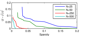
Figure 1: Comparison of sparse controllers to the optimal LQR control law $J^{*}$ for varying levels of sparsity on the mass-spring system.

We begin by characterizing the trade-off between sparsity and system performance by sweeping across 100 logarithmically spaced values of $\lambda$. For the system with $N=50$ springs, the results shown in Figure 1 are nearly identical to those reported by [12], although their methodology includes an additional loop and iteratively solving a series of reweighted $\ell_{1}$ problems. For all systems, the leftmost point represents a control law based almost entirely on local information—although the results shown penalize the elements of $K$ uniformly, we also found that by regularizing just the elements of $K$ corresponding to nonlocal feedback we were able to find stable local control laws in all examples. As $\lambda$ decreases, the algorithm finds controllers that quickly approach the performance of LQR and in the smallest example we require a controller with 18% nonzero elements to be within $0.1\%$ of the LQR performance; in the largest example we require only and 4.0% sparsity to reach this level. This demonstrates the trend that we anticipate: larger systems require comparatively sparser controllers for optimal performance.

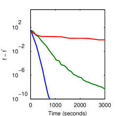
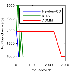
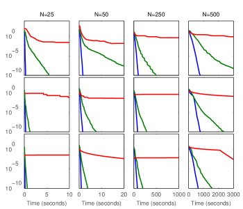
Figure 2: Convergence of algorithms on mass-spring system with $N=500$ and $\lambda=10$ (top left); the sparsity found by each algorithm for the same system (top right); and across many settings with one column per example and rows corresponding to different settings of $\lambda$ with $\lambda_{1}=[10,10,1,1]$, $\lambda_{2}=[1,1,0.1,0.1]$ and $\lambda_{3}=[0.1,0.1,0.01,0.01]$ (bottom).

Next we compare running times of each algorithm by fixing $\lambda$ and considering the convergence of the objective value $f$ at each iteration to the (local) optimum $f^{*}$. Figure 2 shows three such fixed $\lambda$ settings corresponding to the levels of sparsity of interest in the mass-spring system and we in all settings that the Newton-CD method converges far more quickly than other methods. In the largest system considered ($N=500$) with $\lambda=0.1$ (top left), it converges to a solution accurate to $10^{-8}$ in less than 11 minutes whereas ADMM has not reached an accuracy of $10^{-1}$ after over two hours. In addition, the sparsity pattern in the intermediate solutions do not typically correspond to that of the $\ell_{1}$ solution, as can be seen in Figure 2 (top right). For smaller examples, ISTA is competitive but as the size of the system grows, the many iterations that it requires to converge become more expensive, a behavior that is highlighted in the convergence for the $N=500$ system (rightmost column). Finally, we note that Newton-CD performs especially well on $\lambda$ corresponding to sparse solutions (top row) due to the active set method exploiting sparsity in the solution.

In addition to solving the $\ell_{1}$ problem, the Newton-CD method can also be used for the polishing step of finding the optimal controller with a fixed sparsity structure. In Figure 3, we compare Newton-CD to the conjugate gradient approach of [12] which can be seen as a Newton-Lasso method for the special case of $\Lambda$ with entries $0$ or $\infty$. Here we see that performance on the polishing step is comparable with both methods converging quickly and using the same number of outer loop iterations. We note that the conjugate gradient approach could also be extended to work for general $\Lambda$ by using an orthant-based approach (for example, see [33]), but we do not pursue that direction in this work.

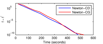
Figure 3: Convergence of Newton methods on the polishing step for the mass-spring system with $N=500$ and $\lambda=100$.

IV-B Wide-area control in power systems

Following [34], which applied the sparse optimal control framework and the ADMM algorithm to this same problem, our next examples consider the task of controlling inter-area oscillations in a power network via wide-area control. These examples highlight the computational benefits of our algorithmic approach even more so than the synthetic examples above.

To briefly introduce the domain ([34] explains the overall setup in more detail), we are concerned here with the problem of frequency regulation in a AC transmission grid. We employ a linearized approximation where for each generation the system state consists of the power angle $\theta_{i}$, the mismatch between the rotational velocity and the reference rotational velocity $\omega_{i}-\omega^{\mathrm{ref}}$, as well as a number of additional states $x_{i}$ characterizing the exciters, governors, and/or power system stabilizer (PSS) control loops at each generator (typically operating on much faster time scale). The system dynamics can be written generically as

$$\begin{split}\dot{\theta}&=\omega-\omega^{\mathrm{ref}}\\ \dot{\omega}&=(Y_{GG}-Y_{GL}Y_{LL}^{-1}Y_{LG})\theta+f(x)\end{split}$$ (40)

where $Y$ is an approximate DC power flow susceptance matrix; $G$ and $L$ are the generator and load nodes; and $f(x)$ denotes the local control dynamics. Importantly, there is a coupling between the generators induced by the network dynamics, which can create oscillatory modes that cannot easily be stabilized by local control alone. The control actions available to the system effectively involve setting the operating points for the inner loops of the power system stabilizers.

The examples we use here are all drawn from the Power Systems Toolbox, in particular the MathNetEig package, which provides a set of routines for describing power networks, generators, exciters and power system stabilizers, potentially at each generator node, and also has routines for analytically deriving the resulting linearized systems. We evaluate our approach on all the larger examples included with this toolbox, as well as the New England 39 bus system used in [34] (which is similar to the 39 bus system included in the power system toolbox, but which includes power system stabilizers at 9 of the 10 generators, limits the type of external control applied to each PSS, and which allows for no control at one of the generators). To create a somewhat larger system than any of those included in the toolbox, we also modify the PST 50 machine system to include power system stabilizers at each node, resulting in a $n=500$ state system to regulate with our sparse control algorithm.

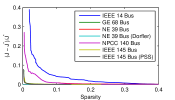
Figure 4: Comparison of performance to LQR solution for varying levels of sparsity on wide-area control in power networks.

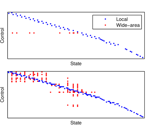
Figure 5: Sparsity patterns for wide-area control in the NPCC 140 Bus power system: the sparsest stable solution found (top) and the sparsest solution achieving performance within 10% of optimal (bottom)

.

As in the previous example, we begin by considering the sparsity/performance trade-off by varying the regularization parameter $\lambda$, shown in Figure 4. Here we see that for several powers systems under consideration, near optimal performance is achieved by an extremely sparse controller depending almost exclusively on local information. As in the mass-spring system, in addition to $\Lambda$ with uniform weights, we also used a structured $\Lambda$ to find local controllers; here were able to find stable local control laws for every example with the exception of PST 48. For this power system, we show the sparsity pattern of the sparsest stable controller in Figure 5 along with that of the controller achieving performance within 10% of the full LQR optimum. Finally, we note that in general the larger power systems admit controllers with relatively more sparsity as was the case in the mass-spring system.

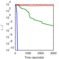
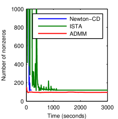
Figure 6: Convergence of algorithms on IEEE 145 Bus (PSS) wide-area control example with $\lambda=100$ (left) and the number of nonzeros in the intermediate solutions (right).

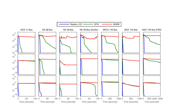
Figure 7: Convergence of algorithms on wide-area control across all power systems with three choices of $\lambda$ corresponding to performance within $10\%$, $1\%$ and $0.1\%$ of LQR. Columns correspond to power systems and rows correspond to different choices of $\lambda$ with largest on top.

Computationally, we consider the convergence on the largest power system example in Figure 6 and observe a dramatic difference between Newton-CD and previous algorithms: Newton-CD has converged to an accuracy better than $10^{-8}$ in less than 173 seconds while ADMM is not within $10^{3}$ after over an hour. In addition, the sparsity pattern of the intermediate solutions found by ADMM is significantly different than that of Newton-CD and ISTA which have converged to the $\ell_{1}$ regularized solution with much higher accuracy. In Figure 7 we consider convergence across all power systems with three values of $\lambda$ chosen such that the resulting controllers have performance within $10\%$, $1\%$ and $0.1\%$ of LQR. Here we see similar results as in the large system with Newton-CD converging faster across all examples and choices of $\lambda$ and the differences being orders of magnitude in many cases. We note that algorithm benefits significantly from a high level of sparsity for these choices of $\lambda$ since for most power systems considered, the controller achieving performance within $0.1\%$ of LQR is still quite sparse.

V Conclusion

In this paper we develop a fast second order algorithm for the sparse LQR problem with the goal of designing sparse control laws for large distributed systems with thousands of nodes. Intuitively we expect that distributed systems characterized by sparsity in the dynamics (e.g. neighbor interactions in the mass-spring system and the graph Laplacian in power networks) can be well controlled with only limited information sharing; we see in the experimental results that as these systems increase in size, they are controllable by laws that become increasingly sparse. Computationally, the design of efficient algorithms is complicated by both the Lyapunov equations which give rise to $O(n^{3})$ complexity, and the nonsmooth $\ell_{1}$ penalty. Our work limits this complexity through an efficient Newton-Lasso algorithm reducing the time required to solve the $\ell_{1}$ problem to that of previous results with fixed structure. However, the $O(n^{3})$ complexity inherent in the Lyapunov equations pose a significant bottleneck to scaling to systems beyond thousands of nodes and thus decomposition methods allowing smaller subproblems to be solved independently are an interesting direction for future research.

References

- [1] B. D. Anderson and J. B. Moore, Optimal control: linear quadratic methods. Prentice Hall Englewood Cliffs, NJ, 1990, vol. 1.
- [2] V. D. Blondel and J. N. Tsitsiklis, “A survey of computational complexity results in systems and control,” Automatica, vol. 36, no. 9, pp. 1249–1274, 2000.
- [3] H. S. Witsenhausen, “A counterexample in stochastic optimum control,” SIAM Journal on Control, vol. 6, no. 1, pp. 131–147, 1968.
- [4] R. Lau, R. Persiano, and P. Varaiya, “Decentralized information and control: A network flow example,” Automatic Control, IEEE Transactions on, vol. 17, no. 4, pp. 466–473, 1972.
- [5] S.-H. Wang and E. Davison, “On the stabilization of decentralized control systems,” Automatic Control, IEEE Transactions on, vol. 18, no. 5, pp. 473–478, 1973.
- [6] N. Sandell Jr, P. Varaiya, M. Athans, and M. Safonov, “Survey of decentralized control methods for large scale systems,” Automatic Control, IEEE Transactions on, vol. 23, no. 2, pp. 108–128, 1978.
- [7] C.-H. Fan, J. L. Speyer, and C. R. Jaensch, “Centralized and decentralized solutions of the linear-exponential-gaussian problem,” Automatic Control, IEEE Transactions on, vol. 39, no. 10, pp. 1986–2003, 1994.
- [8] X. Qi, M. V. Salapaka, P. G. Voulgaris, and M. Khammash, “Structured optimal and robust control with multiple criteria: A convex solution,” Automatic Control, IEEE Transactions on, vol. 49, no. 10, pp. 1623–1640, 2004.
- [9] M. Rotkowitz and S. Lall, “A characterization of convex problems in decentralized control,” Automatic Control, IEEE Transactions on, vol. 51, no. 2, pp. 274–286, 2006.
- [10] P. Shah and P. Parrilo, “H2-optimal decentralized control over posets: A state space solution for state-feedback,” in Decision and Control (CDC), 2010 49th IEEE Conference on, 2010, pp. 6722–6727.
- [11] J. Swigart and S. Lall, “Decentralized control,” Networked Control Systems. Lecture Notes in Control and Information Sciences, vol. 406, pp. 179–201, 2011.
- [12] F. Lin, M. Fardad, and M. Jovanovic, “Design of optimal sparse feedback gains via the alternating direction method of multipliers,” Automatic Control, IEEE Transactions on, vol. 58, no. 9, pp. 2426–2431, 2013.
- [13] S. Schuler, P. Li, J. Lam, and F. Allgöwer, “Design of structured dynamic output-feedback controllers for interconnected systems,” International Journal of Control, vol. 84, no. 12, pp. 2081–2091, 2011.
- [14] S. Schuler, U. Münz, and F. Allgöwer, “Decentralized state feedback control for interconnected systems with application to power systems,” Journal of Process Control, 2013.
- [15] K. Dvijotham, E. Theodorou, E. Todorov, and M. Fazel, “Convexity of optimal linear controller design,” in Proceedings of the Control and Decision Conference, 2013.
- [16] K. Dvijotham, E. Todorov, and M. Fazel, “Convex structured controller design,” CoRR, vol. abs/1309.7731, 2013.
- [17] S. Boyd, N. Parikh, E. Chu, B. Peleato, and J. Eckstein, “Distributed optimization and statistical learning via the alternating direction method of multipliers,” Foundations and Trends® in Machine Learning, vol. 3, no. 1, pp. 1–122, 2011.
- [18] R. Tibshirani, “Regression shrinkage and selection via the lasso,” Journal of the Royal Statistical Society. Series B (Methodological), pp. 267–288, 1996.
- [19] D. L. Donoho, “Compressed sensing,” Information Theory, IEEE Transactions on, vol. 52, no. 4, pp. 1289–1306, 2006.
- [20] E. J. Candes, J. K. Romberg, and T. Tao, “Stable signal recovery from incomplete and inaccurate measurements,” Communications on pure and applied mathematics, vol. 59, no. 8, pp. 1207–1223, 2006.
- [21] B. Efron, T. Hastie, I. Johnstone, and R. Tibshirani, “Least angle regression,” The Annals of statistics, vol. 32, no. 2, pp. 407–499, 2004.
- [22] K. Koh, S.-J. Kim, and S. P. Boyd, “An interior-point method for large-scale l1-regularized logistic regression.” Journal of Machine learning research, vol. 8, no. 8, pp. 1519–1555, 2007.
- [23] P. Tseng and S. Yun, “A coordinate gradient descent method for nonsmooth separable minimization,” Mathematical Programming, vol. 117, no. 1-2, pp. 387–423, 2009.
- [24] R. H. Byrd, J. Nocedal, and F. Oztoprak, “An Inexact Successive Quadratic Approximation Method for Convex L-1 Regularized Optimization,” ArXiv e-prints, Sep. 2013.
- [25] C.-J. Hsieh, M. A. Sustik, I. S. Dhillon, and P. D. Ravikumar, “Sparse inverse covariance matrix estimation using quadratic approximation,” CoRR, vol. abs/1306.3212, 2013.
- [26] M. Wytock and J. Z. Kolter, “Sparse gaussian conditional random fields: Algorithms, theory, and application to energy forecasting,” in Proceedings of the International Conference on Machine Learning, 2013.
- [27] V. Simoncini, “Computational methods for linear matrix equations,” 2013.
- [28] L. Greengard and V. Rokhlin, “A fast algorithm for particle simulations,” Journal of computational physics, vol. 73, no. 2, pp. 325–348, 1987.
- [29] R. A. Horn and C. R. Johnson, Matrix analysis. Cambridge university press, 2012.
- [30] T. Rautert and E. W. Sachs, “Computational design of optimal output feedback controllers,” SIAM Journal on Optimization, vol. 7, no. 3, pp. 837–852, 1997.
- [31] A. Gerasoulis, “A fast algorithm for the multiplication of generalized hilbert matrices with vectors,” Mathematics of Computation, vol. 50, no. 181, pp. 179–188, 1988.
- [32] V. Pan, M. A. Tabanjeh, Z. Chen, E. Landowne, and A. Sadikou, “New transformations of cauchy matrices and trummer’s problem,” Computers & Mathematics with Applications, vol. 35, no. 12, pp. 1–5, 1998.
- [33] P. Olsen, F. Oztoprak, J. Nocedal, and S. Rennie, “Newton-like methods for sparse inverse covariance estimation,” in Advances in Neural Information Processing Systems 25, 2012, pp. 764–772.
- [34] F. Dörfler, M. R. Jovanovic, M. Chertkov, and F. Bullo, “Sparsity-Promoting Optimal Wide-Area Control of Power Networks,” ArXiv e-prints, Jul. 2013.