Dilaton gravity, (quasi-) black holes, and scalar charge

Abstract

Electrically charged dust is considered in the framework of Einstein-Maxwell-dilaton gravity with a Lagrangian containing the interaction term $P(\chi)F_{\mu\nu}F^{\mu\nu}$, where $P(\chi)$ is an arbitrary function of the dilaton scalar field $\chi$, which can be normal or phantom. Without assumption of spatial symmetry, we show that static configurations exist for arbitrary functions $g_{00}=\exp(2\gamma(x^{i}))$ ($i=1,2,3$) and $\chi=\chi(\gamma)$. If $\chi={\rm const}$, the classical Majumdar-Papapetrou (MP) system is restored. We discuss solutions that represent black holes (BHs) and quasi-black holes (QBHs), deduce some general results and confirm them by examples. In particular, we analyze configurations with spherical and cylindrical symmetries. It turns out that cylindrical BHs and QBHs cannot exist without negative energy density somewhere in space. However, in general, BHs and QBHs can be phantom-free, that is, can exist with everywhere nonnegative energy densities of matter, scalar and electromagnetic fields.

I Introduction

Studies of self-gravitating systems with spherical symmetry are one of the most important applications of gravity theories, above all because they are directly related to one of the most notable objects in nature: the stars. General Relativity (GR) modifies the usual predictions of the Newtonian theory for static, spherically symmetric systems in many different ways, and at the same time makes possible the emergence of a new class of structures, black holes (BHs), collapsed objects that can represent the final fate of supermassive stars. The crucial concept characterizing BHs is the existence of an event horizon, a hypersurface isolating the internal region of a collapsed object from the external region with distant observers living in almost flat space-time.

The vacuum static, spherically symmetric solution of GR, known as the Schwarzschild solution, describes the simplest BH. Its generalizations are the charged static black hole represented by the Reissner-Nordtström (RN) solution, rotating (Kerr) and charged rotating (Kerr-Newman) black holes h-e ; fro-nov . In the non-vacuum case, one important type of configurations are those of static charged dust, represented by the Majumdar-Papapetrou (MP) solution majumdar ; papa : it represents an equilibrium between gravitational attraction and electric repulsion.

An important feature of the MP system is that it actually does not need spherical or any other spatial symmetry for its existence: the static equilibrium between gravity and electric forces allows for any spatial shape of a charged dust cloud provided the mass to charge density ratio takes everywhere the proper value: $\rho_{e}/\rho_{m}=\pm 1$ in natural units ($c=G=1$, $c$ being the speed of light and $G$ the Newtonian gravitational constant).

The MP systems have been revived in quite a new context connected with the so-called quasi-black holes (QBHs) [5–12]. These are systems on the threshold of forming a black hole horizon but the horizon does not form. This becomes possible since equilibrium between gravitational attraction and electrostatic repulsion exists for any size of the object close to the horizon radius. From the viewpoint of a distant observer, the system looks indistinguishable from a true BH, although in the vicinity of this would-be horizon their properties are very different.

All these examples are implemented in the pure GR context, using at most the electromagnetic field as an external source. Less known systems are those which include scalar fields. One initial reason for ignoring scalar fields were doubts on the existence of fundamental scalar particles in nature. The recently announced discovery of the Higgs boson may invalidate these doubts. Anyway, BHs with scalar fields have been considered many times in the literature since scalar fields are the simplest possible sources of the gravitational field.

Scalar fields minimally coupled to gravity were considered for the first time, to our knowledge, by Fisher fish who found a static, spherically symmetric solution to the Einstein-massless scalar field equations. A counterpart of Fisher’s solution for massless scalar fields with a wrong sign of the kinetic energy (the so-called phantom scalar) was found by Bergmann and Leipnik pha-57 , and both solutions were repeatedly re-discovered afterwards. Later, a general study of spherically symmetric scalar + gravity systems, including a possible non-minimal coupling (hence in the context of a general scalar-tensor theory of gravity rather than pure GR), was undertaken in br73 , where some nontrivial new configurations corresponding to BH and wormhole structures were identified. Among special cases thereof are neutral and charged BHs boch and wormholes with a conformally coupled scalar field as well as the so-called Ellis wormholes (described by the simplest case of the Bergmann-Leipnik solution pha-57 ) and wormholes in the Brans-Dicke scalar-tensor theory BD in the case where the coupling constant $\omega$ is smaller than $-3/2$. These results were somehow extended later by identifying the so-called cold BHs, i.e., BHs containing scalar charges, exhibiting zero surface gravity and infinite horizon surface areas cold1 ; cold2 ; cold-q . In general, to obtain such cold BHs, the scalar field must have negative kinetic energy, that is, it must be phantom and violate the standard energy conditions.

The emergence of string theories as a possible candidate for a unified theory of all interactions has led to new ingredients with important consequences for the studies of structures like BHs. String theory in its effective low-energy formulation predicts the existence of scalar and gauge fields with a nontrivial coupling between them. More precisely, the string effective action contains a scalar field, the dilaton, nonmiminally coupled to gravity. If the electromagnetic field is kept in the Neveu-Schwarz sector of the tree-level string action, re-expressed in the Einstein frame, the coupling between the dilatonic and electromagnetic fields appears in an exponential form, as ${\,\rm e}^{2\lambda\chi}F_{\mu\nu}F^{\mu\nu}$, where $\chi$ is the dilaton. However, taking into account the loop expansion of string theory, one can obtain other (and hard-to-identify) coupling functions $P(\chi)$ instead of ${\,\rm e}^{2\lambda\chi}$ dam1 ; dam2 . This motivates studies of the Einstein-Maxwell-dilaton (EMD) system with an arbitrary function $P(\chi)$.

Concerning exact static, spherically symmetric solutions for the EMD system, to the best of our knowledge, the solutions for $P(\chi)={\,\rm e}^{2\lambda\chi}$ were obtained for the first time in BSh-77 ; BSh-77e , where also a family of what we now know as “dilatonic black holes” dbh1 ; dbh2 ; dbh3 was singled out. Later on, the EMD system with an arbitrary function $P(\chi)$ was considered BMsh-78 ; BMsh-78e ; ann-79 in attempts to obtain a nonsingular, classical, purely field particle model. The conditions were revealed under which a regular center in the EMD system is possible, and an explicit example of such a regular model was built.

More general studies, inspired by achievements in various field limits of supergravity and superstring theories, were undertaken in the 90s and involved extensions of the EMD system to space-times of arbitrary dimensions with products of multiple factor spaces and, as material sources of gravity, a number of scalar dilatonic fields ($\chi^{a}$) and a number of antisymmetric forms of different ranks ($F_{s}$), of which the electromagnetic field $F_{\mu\nu}$ is the simplest representative, see bra-r1 ; bra-r2 for reviews. Various classes of exact solutions were found, among them many static, spherically symmetric ones (see, e.g., kb95 ; bra1 ; bra2 ; bra3 and references therein), of which the most well-known are the so-called “black branes” with different configurations of extra factor spaces. It should be noted that in all these studies the interaction between scalar and antisymmetric form fields was assumed in the exponential form, like $F_{s}^{2}\exp(\lambda_{sa}\chi^{a})$, where $\lambda_{sa}$ is a matrix with constant real elements.

Returning to four dimensions with a single scalar interacting exponentially with a single electromagnetic field, we can say that the most complete study of this static, spherically symmetric EMD system was carried out in clem1 where the initial action was not restricted to only a string-inspired coupling and included the possibility of a phantom behavior of both scalar and Maxwell fields. Many new BH structures were revealed, asymptotically flat or not, but all of them required the existence of phantom fields, either in the scalar or in the electromagnetic sector (or in both). All these new structures have properties similar to cold black holes in the sense that their surface gravity is zero. (For a study of a perfect-fluid source of vacuum EMD fields see yaz ).

Such an extremal nature of these phantom EMD BHs leads to a speculation that structures like QBHs, previously based on the Majumdar-Papapetrou solution of GR, could be implemented for such more general phantom BHs: since in all these cases the scalar field is phantom, it is possible to conjecture on a QBH configuration supported by an attractive or repulsive effect of a scalar field in addition to electric repulsion. This idea has been initially considered in a PhD thesis of one of the co-authors of the present work, Robson Silveira, who died in 2009 before completing the proposed study. Before his death, he was able to obtain some initial results indicating that such scalar QBHs are really possible and designing some of their main properties. In particular, he found QBHs supported by only a phantom scalar field. The goal of the present paper is to report on a more general analysis completing his findings.

We include into consideration all ingredients which were earlier discussed separately: matter (electrically and scalarly charged dust), an electromagnetic field and a scalar field interacting with it in a dilatonic manner. We make some general observations on possible equilibrium configurations (to be called dilatonic MP, or DMP systems) and pay special attention to BHs and QBHs supported by certain electric and scalar charge distributions. In particular, we try to find phantom-free configurations, i.e., those able to exist with positive-definite energy densities of matter and both fields. Some of the results have been already briefly presented in our previous paper we-14 .

The paper is organized as follows. Section II presents the general EMD field equations, Section III specializes them for static systems to be considered, Section IV describes their two simple special cases, one of them being that of MP systems, the other its purely scalar counterpart. In Section V we make some observations about general EMD systems without symmetry and determine, in particular, the necessity of a nonzero scalar charge density for their existence. Section VI is devoted to general properties of spherically symmetric systems, including the conditions at a regular center, at a horizon, and at flat spatial infinity. We also obtain a balance condition between the mass and integral electric and scalar charges, applicable to any asymptotically flat systems, not necessarily spherical ones. The general properties of spherically symmetric BHs and QBHs are also described, including limiting transitions between them. In Section VII we give some examples of BHs and QBHs, showing, in particular, that both are possible without invoking phantom matter or fields. Section VIII deals with the properties of cylindrically symmetric configurations. Lastly, Section IX summarizes and discusses the results.

II Basic equations

Consider the Lagrangian (putting $c=G=1$)

$$L=\frac{1}{16\pi}\biggl{[}R+2\varepsilon(\partial\chi)^{2}-F^{2}P(\chi)\biggr{]}+L_{m}+A_{\mu}j^{\mu}+J\chi,$$ (1)

where $\varepsilon=\pm 1$ ($\varepsilon=1$ for a normal scalar field $\chi$), $L_{m}$ is the Lagrangian of matter, $J$ is the scalar charge density, $F^{2}\equiv F^{\alpha\beta}F_{\alpha\beta}$ ($F_{\mu\nu}=\partial_{\mu}A_{\nu}-\partial_{\nu}A_{\mu}$, the electromagnetic field), $j^{\mu}=\rho_{e}u^{\mu}$ is the 4-current, $u^{\mu}$ is the 4-velocity. For generality, and also to provide correspondence with clem1 ; clem2 , we do not fix the sign of $P(\chi)$.

The corresponding field equations are

$$4\varepsilon\Box\chi+F^{2}P_{\chi} = 16\pi J,$$ (2)

$${}\nabla_{\alpha}(P(\chi)F^{\alpha\mu}) = -4\pi j^{\mu},$$ (3)

$${}G_{\mu}^{\nu} = -8\pi T_{\mu}^{\nu},$$ (4)

where $P_{\chi}:=dP/d\chi$ and $T_{\mu}^{\nu}$ is the summed stress-energy tensor (SET) of matter and the fields:

$$T_{\mu}^{\nu} = T_{\mu}^{\nu}{}_{(s)}+T_{\mu}^{\nu}{}_{(e)}+T_{\mu}^{\nu}{}_{(m)},$$ (5)

$${}8\pi T_{\mu}^{\nu}{}_{(s)} = \varepsilon[2\partial_{\mu}\chi\partial^{\nu}\chi-\delta_{\mu}^{\nu}(\partial\chi)^{2}],$$ (6)

$${}8\pi T_{\mu}^{\nu}{}_{(e)} = P(\chi)[-2F_{\mu\alpha}F^{\nu\alpha}+{{\textstyle\frac{1}{2}}}\delta_{\mu}^{\nu}F^{2}],$$ (7)

$${}T_{\mu}^{\nu}{}_{(m)} = \rho_{m}u_{\mu}u^{\nu}.$$ (8)

The condition $\nabla_{\nu}T_{\mu}^{\nu}=0$ leads to the equations of motion for dust particles (using Eqs. (2) and (3) to eliminate the second-order derivatives)

$$u_{\mu}\nabla_{\alpha}(\rho_{m}u^{\alpha})+\rho_{m}u^{\alpha}\nabla_{\alpha}u_{\mu}-F_{\mu\alpha}j^{\alpha}+J\chi_{,\mu}=0.$$ (9)

Its contraction with $u^{\mu}$ leads to the generalized continuity equation

$$\nabla_{\alpha}(\rho_{m}u^{\alpha})+J\chi_{,\alpha}u^{\alpha}=0.$$ (10)

With (10), Eq. (9) takes the form

$$\rho_{m}u^{\alpha}\nabla_{\alpha}u_{\mu}-F_{\mu\alpha}j^{\alpha}+J(\chi_{,\mu}-u_{\mu}u^{\alpha}\chi_{,\alpha})=0.$$ (11)

III Static equilibrium

The assumptions of static equilibrium are: the metric

$$ds^{2}={\,\rm e}^{2\gamma}dt^{2}-{\,\rm e}^{-2\gamma}h_{ik}dx^{i}dx^{k},$$ (12)

and only $F_{0i}=-F_{i0}=\phi_{i}$ are nonzero among $F_{\mu\nu}$ (only the electric field is present); $\gamma$, $h_{ik}$, $\phi$, $\chi$ are functions of $x^{i}$, $i=1,2,3$. We use the notations $\gamma_{i}=\partial_{i}\gamma$, $\phi_{i}=\partial_{i}\phi$ etc. The spatial indices are raised and lowered with the metric $h_{ik}$ and its inverse $h^{ik}$, and the 4-velocity is $u^{\mu}=\delta^{\mu}_{0}{\,\rm e}^{-\gamma}$.

Eqs. (2) and (3) take the form

$$2\varepsilon{\,\rm e}^{2\gamma}\Delta\chi+P_{\chi}\phi_{i}\phi^{i} = -8\pi J,$$ (13)

$${}\nabla_{i}\left({\,\rm e}^{-2\gamma}P\phi^{i}\right) = 4\pi\rho_{e}{\,\rm e}^{-3\gamma},$$ (14)

where $\nabla_{i}$ and the Laplace operator $\Delta=\nabla_{i}\nabla^{i}$ are defined in terms of the metric $h_{ik}$.

The nonzero components of the Ricci and Einstein tensors are

$$R^{0}_{0} = -{\,\rm e}^{2\gamma}\Delta\gamma,$$

$${}R^{k}_{i} = -{\,\rm e}^{2\gamma}(^{h}R^{k}_{i}+2\gamma_{i}\gamma^{i}-\delta^{k}_{i}\Delta\gamma);$$ (15)

$${}G^{0}_{0} = {\,\rm e}^{2\gamma}({{\textstyle\frac{1}{2}}}^{h}R+\gamma^{i}\gamma_{i}-2\Delta\gamma),$$

$${}G_{i}^{k} = {\,\rm e}^{2\gamma}(-^{h}R_{i}^{k}+{{\textstyle\frac{1}{2}}}^{h}R\delta_{i}^{k}-2\gamma_{i}\gamma^{k}+\delta_{i}^{k}\gamma_{j}\gamma^{j}),$$ (16)

where ${}^{h}R^{k}_{i}$ and ${}^{h}R$ are the Ricci tensor and scalar obtained from the metric $h_{ik}$.

The nonzero components of the SETs are

$$8\pi T^{0}_{0}{}_{(s)} = \varepsilon{\,\rm e}^{2\gamma}\chi_{i}\chi^{i},$$

$${}8\pi T_{i}^{k}{}_{(s)} = \varepsilon{\,\rm e}^{2\gamma}(-2\chi_{i}\chi^{k}+\delta_{i}^{k}\chi_{j}\chi^{j});$$ (17)

$$8\pi T^{0}_{0}{}_{(e)} = P(\chi)\phi_{i}\phi^{i},$$

$${}8\pi T_{i}^{k}{}_{(e)} = P(\chi)(2\phi_{i}\phi^{k}-\delta_{i}^{k}\phi_{j}\phi^{j});$$ (18)

$$T_{\mu}^{\nu}{}_{(m)} = \rho_{m}\mathop{\rm diag}\nolimits(1,\ 0,\ 0,\ 0).$$ (19)

Let us now assume that the spatial metric $h_{ik}$ is flat (but not necessary written in Cartesian coordinates in which $h_{ik}=\delta_{ik}$). Then ${}^{h}R_{i}^{k}=0$, and the Einstein equations $R^{0}_{0}=\ldots$ and $R_{i}^{k}=\ldots$ read

$${\,\rm e}^{2\gamma}\Delta\gamma = P\phi_{i}\phi^{i}+4\pi\rho_{m},$$ (20)

$${}{\,\rm e}^{2\gamma}[2\gamma_{i}\gamma^{k}-\delta_{i}^{k}\Delta\gamma] = -4\pi\rho_{m}\delta_{i}^{k}+P[2\phi_{i}\phi^{k}-\delta_{i}^{k}\phi_{j}\phi^{j}]-2\varepsilon{\,\rm e}^{2\gamma}\chi_{i}\chi^{k}.$$ (21)

Excluding $\rho_{m}$ from (21), we obtain the first-order equation

$${\,\rm e}^{2\gamma}(\gamma_{i}\gamma^{k}+\varepsilon\chi_{i}\chi^{k})=P\,\phi_{i}\phi^{k}$$ (22)

which does not contain the densities, hence it holds both in vacuum and in matter.

Since in our static system $\rho_{m}u^{\alpha}\nabla_{\alpha}u_{\mu}$ reduces to $-\rho_{m}\gamma_{i}$ (with the index $\mu=i$), the equation of motion (11) now leads to the equilibrium condition

$$\rho_{m}\gamma_{i}-\rho_{e}\phi_{i}{\,\rm e}^{-\gamma}=J\chi_{i};$$ (23)

the continuity equation takes the usual form $\nabla_{\mu}(\rho_{m}u^{\mu})=0$ and holds automatically.

IV The Majumdar-Papapetrou system and its scalar counterpart

Let us briefly recall the classical case $\chi\equiv 0$, $P\equiv 1$, that is, electrically charged dust, the Majumdar-Papapetrou (MP) system. The scalar equation (13) is absent, while Eq. (22) gives

$${\,\rm e}^{2\gamma}\,\gamma_{i}\gamma^{k}=\phi_{i}\phi^{k}.$$ (24)

In particular, we can write ${\,\rm e}^{2\gamma}\gamma_{1}^{2}=\phi_{1}^{2}$ and similar relations for the derivatives in $x^{2}$ and $x^{3}$, whose integration leads to

$${\,\rm e}^{\gamma} = \pm\phi+C_{1}(x^{2},x^{3})$$ (25)

$$= \pm\phi+C_{2}(x^{1},x^{3})$$

$$= \pm\phi+C_{3}(x^{1},x^{2})$$

whence it follows $C_{1}=C_{2}=C_{3}={\rm const}=1$ according to the boundary conditions that $\phi\to 0$ and ${\,\rm e}^{\gamma}\to 1$ at spatial infinity. Thus we have

$$\pm\phi={\,\rm e}^{\gamma}-1.$$ (26)

Using Eqs. (14) and (20) as expressions for $\rho_{e}$ and $\rho_{m}$, we then obtain $\rho_{\,\rm e}=\pm\rho_{m}$ and

$$4\pi\rho_{m}=\pm 4\pi\rho_{e}=-{\,\rm e}^{3\gamma}\Delta({\,\rm e}^{-\gamma}).$$ (27)

Eqs. (22) and (23) hold automatically. The charge and mass densities, equal in absolute value, are thus (up to the factor ${\,\rm e}^{3\gamma}$) sources of the effective gravitational potential ${\,\rm e}^{-\gamma}$. On the contrary, for each smooth $\gamma=\gamma(x^{i})$ one finds the proper charge and mass distribution able to be its source.

Noteworthy, it is not necessary here to assume a relationship between the functions $\phi(x^{i})$ and $\gamma(x^{i})$, it has emerged automatically from the equilibrium conditions.

A somewhat similar situation is observed if we put, on the contrary, $\phi={\rm const}\ \Rightarrow\ F_{\mu\nu}\equiv 0$. In this case, Eq. (22) reads $\gamma_{i}\gamma^{k}+\varepsilon\chi_{i}\chi^{k}=0$, whence it follows $\varepsilon=-1$ (an equilibrium is only possible with a phantom scalar field, which confirms its repulsive nature) and

$$\pm\chi_{i}=\gamma_{i}.$$ (28)

Then Eqs. (20) and (23) express the densities $\rho_{m}$ and $J$ in terms of $\gamma(x^{i})$:

$$\pm 4\pi J=4\pi\rho_{m}={\,\rm e}^{2\gamma}\Delta\gamma.$$ (29)

As in the MP system, for each smooth $\gamma=\gamma(x^{i})$ one finds the proper scalar charge and mass density distributions able to be its source.

In both cases (27) and (29) one can consider a set of point sources instead of their continuous distribution. However, the nature of these point sources is quite different. Thus, in the MP system the field of a point source satisfies $\Delta{\,\rm e}^{-\gamma}=0$, whence

$${\,\rm e}^{\gamma}=x/(m+x),\hskip 28.45274ptx:=(x_{i}x^{i})^{1/2},$$ (30)

under the boundary condition $\gamma\to 0$ as $x\to\infty$, and $m$ has the meaning of the Schwarzschild mass. As is well known, it is an extreme Reissner-Nordström black hole with a horizon at $x=0$, at which the spherical radius $r=x{\,\rm e}^{-\gamma}$ is equal to $m$.

Unlike that, in the Einstein-scalar field system Eq. (29) implies $\Delta\gamma=0$ outside a source, hence, under the same boundary condition, $\gamma=-m/x$, and the source at $x=0$ is a naked singularity.

V General static configurations

In the general static case we have the following independent equations: (13), (14), (20) and (22). The tensor equation (22) implies that $\gamma$, $\chi$ and $\phi$ are functionally related, so that, if $\gamma\neq{\rm const}$, we can put $\phi=\phi(\gamma)$ and $\chi=\chi(\gamma)$.

Indeed, if we assume the contrary, e.g., that $\gamma$ and $\chi$ are functionally independent, then they can be chosen as curvilinear coordinates in 3-space, say, $\gamma=x^{1}$ and $\chi=x^{2}$. Then from the corresponding components of (22) we immediately obtain $\phi_{3}^{2}=0$ and $\phi_{1}\phi_{2}=0$, so that either $\phi=\phi(\gamma)$ or $\phi=\phi(\chi)$. If we take $\phi=\phi(\gamma)$, the $({}_{22})$ component of Eq. (22) makes a contradiction (the l.h.s. is nonzero while the r.h.s. is zero), while if $\phi=\phi(\chi)$, the same happens to the $({}_{11})$ component. Thus our assumption, that $\gamma$ and $\chi$ are independent, is wrong. The same is concluded if we assume independence of $(\gamma,\phi)$ or $(\phi,\chi)$.

Now, assuming $\phi=\phi(\gamma)$ and $\chi=\chi(\gamma)$, Eq. (22) takes the form

$${\,\rm e}^{2\gamma}(1+\varepsilon\chi_{\gamma}^{2})=P\phi_{\gamma}^{2},$$ (31)

where the index $\gamma$ denotes $d/d\gamma$.

Hence we have the following arbitrariness: for any $P(\chi)$ and any 3D profile $\gamma(x^{i})$, even more than that, for an arbitrary scalar field distribution $\chi=\chi(\gamma)$ (up to certain restrictions), we find $\phi(\gamma)$ from (31), and the remaining field equations (13), (14) and (20) give us the mass, electric and scalar charge distributions that support this field configuration. The condition (23) holds due to the Einstein equations.

It is of interest whether or not it is possible to provide $J\equiv 0$, that is, to find configurations without an independent scalar charge, where the $\chi$ field exists only due to its interaction with the electromagnetic field.

Assuming $J\equiv 0$, the equilibrium condition (23) gives

$${\,\rm e}^{\gamma}\rho_{m}=\rho_{e}\,d\phi/d\gamma.$$ (32)

Substituting it into (13), we obtain the following relation:

$$2\varepsilon\chi_{\gamma}\Delta\gamma+\biggl{(}2\varepsilon\chi_{\gamma\gamma}+P_{\chi}\frac{\rho_{m}^{2}}{\rho_{e}^{2}}\biggr{)}\gamma_{i}\gamma^{i}=0.$$ (33)

If we wish to admit configurations with any $\gamma(x^{i})$, then the quantities $\Delta\gamma$ and $\gamma_{i}\gamma^{i}$ are actually independent, and we should require that the factors near them vanish. Then we obtain $\chi={\rm const}$ (the scalar field is trivial) and $P={\rm const}$ (no scalar-electromagnetic interaction), thus actually returning to the MP situation.

We conclude that sufficiently general configurations with $P=P(\chi)$ cannot be obtained without a scalar charge density $J$; however, special solutions to Eq. (33) with particular profiles of $\gamma$ for specific $P(\chi)$ must exist.

Meanwhile, static dust with non-interacting $\chi$ and $F_{\mu\nu}$, corresponding to the special case $P\equiv 1$, can evidently form nontrivial configurations if we admit $J\neq 0$, and some examples will be given below.

In what follows we will try to obtain examples of BH and quasi-BH (QBH) configurations in the simplest cases of spherical and cylindrical symmetries, and of special interest can be those of them where all kinds of matter are “normal”, in particular, $\varepsilon=+1$ and $\rho_{m}\geq 0$. Such an opportunity is not forbidden, but its realization causes some difficulty. The latter is illustrated by the expression for $\rho_{m}$ in terms of $\gamma(x)$ and $\chi(x)$, obtained by combining (20) and (22):

$$4\pi\rho_{m}={\,\rm e}^{2\gamma}(\Delta\gamma-\gamma^{i}\gamma_{i}-\varepsilon\chi^{i}\chi_{i}).$$ (34)

We see that a normal scalar field ($\varepsilon=1$) makes a negative contribution to $\rho_{m}$. If, for example, we choose $\gamma(x^{i})$ satisfying the MP vacuum equation $\Delta({\,\rm e}^{-\gamma})=0$, we obtain simply $\rho_{m}\propto-\varepsilon$.

Nevertheless, since a normal scalar field, like gravity, creates attractive forces between dust particles, it is natural to expect the existence of phantom-free DMP systems where this new attractive component is balanced by an electric charge density larger than in MP systems.

VI Spherically symmetric matter distributions: General features

VI.1 Field equations and asymptotic behavior

In the case of spherical symmetry, the metric (12) with the flat 3-metric $h_{ik}$ takes the form

$$ds^{2}={\,\rm e}^{2\gamma}dt^{2}-{\,\rm e}^{-2\gamma}(dx^{2}+x^{2}d\Omega^{2}),$$ (35)

where $x$ is the usual spherical coordinate in flat 3-space and $d\Omega^{2}$ is the line element on a unit sphere. Our set of equations takes the form

$$2\varepsilon x^{-2}{\,\rm e}^{2\gamma}(x^{2}\chi^{\prime})^{\prime}+P_{\chi}\phi^{\prime}{}^{2} = -8\pi J(x),$$ (36)

$${}x^{-2}\big{(}P{\,\rm e}^{-2\gamma}x^{2}\phi^{\prime}\big{)}^{\prime} = 4\pi\rho_{e}{\,\rm e}^{-3\gamma},$$ (37)

$${}x^{-2}{\,\rm e}^{2\gamma}(x^{2}\gamma^{\prime})^{\prime}-P\phi^{\prime}{}^{2} = 4\pi\rho_{m},$$ (38)

$${}\gamma^{\prime}{}^{2}+\varepsilon\chi^{\prime}{}^{2} = {\,\rm e}^{-2\gamma}P\phi^{\prime}{}^{2},$$ (39)

$${}\rho_{m}\gamma^{\prime}-\rho_{e}\phi^{\prime}{\,\rm e}^{-\gamma} = J\chi^{\prime},$$ (40)

where the prime denotes $d/dx$. The above arbitrariness transforms here into the freedom of choosing the functions $\gamma(x)$ and $\chi(x)$ even if the coupling function $P(\chi)$ has been prescribed from the outset. All other quantities are then found from Eqs. (36)–(40), including the mass, electric and scalar charge distributions that support this field configuration.

It is of interest how to choose the arbitrary functions in order to obtain a starlike configuration with a regular center or a BH. In all cases it is also of interest to see how to provide a phantom-free configuration with $\varepsilon=+1$ and $\rho_{m}\geq 0$. In doing so, we can use Eq. (34) which now takes the form

$$4\pi\rho_{m}={\,\rm e}^{2\gamma}(\gamma^{\prime\prime}+2\gamma^{\prime}/x-\gamma^{\prime}{}^{2}-\varepsilon\chi^{\prime}{}^{2}).$$ (41)

A regular center is obtained in the metric (35) at $x=0$ if and only if

$$\gamma(x)=\gamma_{c}+O(x^{2}),\hskip 28.45274pt\gamma_{c}={\rm const},$$ (42)

and we can use the Taylor expansion

$${\,\rm e}^{2\gamma}\equiv A(x)=A_{0}+{{\textstyle\frac{1}{2}}}A_{2}x^{2}+{\textstyle\frac{1}{6}}A_{3}x^{3}+\cdots,\ \ \ A_{i}={\rm const},\ \ \ A_{0}={\,\rm e}^{2\gamma_{c}}.$$ (43)

According to the field equations, we must also have, as $x\to 0$,

$$\phi(x)=\phi_{c}+O(x^{2}),\hskip 28.45274pt\chi(x)=\chi_{c}+O(x^{2}),$$ (44)

with some constants $\phi_{c}$ and $\chi_{c}$, and this provides finite values of the densities $\rho_{m}$, $\rho_{e}$ and $J$ at the center. The expression (41) then leads to

$$8\pi\rho_{m}=3A_{2}+2A_{3}x+\cdots,$$ (45)

while the $\chi$ field only contributes beginning with $O(x^{2})$. Thus a positive density near the center requires, as usual, that $g_{00}=A(x)$ should have there a minimum.

Horizons. The question on possible Killing horizons inside a charged dust distribution is somewhat more involved. To begin with, in (35) the coordinate $x$ is quasiglobal, which means that it behaves near a horizon in the same way as null Kruskal-like coordinates BR-book , whence follows the requirement that all functions characterizing the system should be analytical at the corresponding point $x=x_{\rm hor}$, hence near the horizon ${\,\rm e}^{2\gamma}\approx B_{0}(x-x_{\rm hor})^{n}$, where $B_{0}={\rm const}>0$ and $n\in{\mathbb{N}}$ is the order of the horizon.

From (35) it is clear that a horizon of finite radius $r_{\rm hor}=x{\,\rm e}^{-\gamma}\big{|}_{x=x_{\rm hor}}$ is only possible with $x_{\rm hor}=0$ and $n=2$ (a double, or extremal horizon). Assuming a simple horizon ($n=1$) at $x=0$, we obtain $r_{\rm hor}=0$, hence a singularity; on the other hand, a higher-order horizon ($n>2$) with any $x_{\rm hor}\geq 0$ corresponds to an infinite radius $r_{\rm hor}$. A continuation beyond such a horizon is possible under some special conditions, and then we are dealing with the so-called “cold BHs”, see cold.

We will not consider here such an unusual opportunity and thus assume that near $x=0$

$${\,\rm e}^{2\gamma}\equiv A(x)={{\textstyle\frac{1}{2}}}A_{2}x^{2}+{\textstyle\frac{1}{6}}A_{3}x^{3}+{\textstyle\frac{1}{24}}A_{4}x^{4}+\cdots,\ \ \ A_{i}={\rm const},\ \ \ A_{2}>0.$$ (46)

Furthermore, the metric analyticity leads, via the Einstein equations, to analytic behaviors of the SET components, in particular, of the quantities $P\phi^{\prime}{}^{2}$ and ${\,\rm e}^{2\gamma}\chi^{\prime}{}^{2}$. The latter means that we can in principle assume

$${\,\rm e}^{\chi}\sim x^{s},\ \ \ s\in{\mathbb{R}}\ \ \ {\rm as}\ \ x\to 0,$$ (47)

so that $\chi^{\prime}\approx s/x$, and only $s=0$ corresponds to $|\chi^{\prime}|<\infty$ as $x\to 0$. It follows from (39) that

$$P\phi^{\prime}{}^{2}\approx{{\textstyle\frac{1}{2}}}A_{2}\varepsilon s^{2}\ \ \ {\rm as}\ \ x\to 0.$$ (48)

Then (38) gives for the matter density

$$2\pi\rho_{m}(0)=-A_{2}\varepsilon s^{2}.$$ (49)

Thus if $s\neq 0$, then $\rho_{m}<0$ in the presence of a normal scalar field ($\varepsilon=+1$) and positive with a phantom one ($\varepsilon=-1$).

The behavior of the other densities, $\rho_{e}$ and $J$, at the horizon depends on the choice of the coupling function $P(\chi)$. Eq. (39) gives $P\phi^{\prime}{}^{2}\to{{\textstyle\frac{1}{2}}}A_{2}(1+\varepsilon s^{2})$ as $x\to 0$, so that the normal, positive sign of the coupling function $P(\chi)$ requires $|s|<1$ if $\varepsilon=-1$. In the special case $\varepsilon=-1$ and $s=1$, we obtain $P\phi^{\prime}(0)^{2}=0$. Let us, however, discuss the generic case where $1+\varepsilon s^{2}\neq 0$.

Assuming that $P(\chi)$ is finite as $x\to 0$ (while ${\,\rm e}^{\chi}\sim x^{s}$), we see that $\phi^{\prime}(0)$ is finite, then from (37) it follows that generically $\rho_{e}\sim x$, but there can be special cases where $\rho_{e}=o(x)$ (if the derivative of the expression in parentheses is zero at $x=0$). From (40) we find that the scalar charge density $J$ is finite at the horizon.

In the important case $P(\chi)={\,\rm e}^{2\lambda\chi}$, $\lambda={\rm const}\neq 0$ (or if $P(\chi)$ behaves like that near the horizon) we have $P\sim x^{2\lambda s}$ as $x\to 0$. From (39) we then find that $\phi^{\prime}\sim x^{-\lambda s}$. Eq. (37) yields in turn $\rho_{e}\sim x^{\lambda s}$, and from (40) it follows that $J$ tends to a finite limit. The requirement $|\rho_{e}|<\infty$ implies $\lambda s>0$ (both $\lambda$ and $s$ are nonzero by assumption), hence $\rho_{e}$ vanishes at the horizon as well as $P(\chi)$, while $\phi^{\prime}$ is infinite.

Let us now discuss the case $s=0$, such that $\chi^{\prime}$ and $\chi$ are finite at the horizon. At small $x$ we then obtain $\rho_{m}\sim x^{2}$, and its sign does not directly correlate with $\varepsilon$. A substitution of (46) into (41) leads to

$$8\pi\rho_{m}=\biggl{(}-\frac{A_{3}^{2}}{12A_{2}}+\frac{A_{4}}{12}-\varepsilon\chi^{\prime}(0)^{2}\biggr{)}x^{2}+O(x^{3}).$$ (50)

From (39) we find that $\phi^{\prime}$ (and hence $\phi$) are finite at the horizon provided that $P(\chi)$ is finite (notably, now the assumption $P(\chi)={\,\rm e}^{2\lambda\chi}$ belongs to this generic case). Eq. (38) then leads, as before, to $\rho_{e}\sim x$ or possibly $\rho_{e}=o(x)$, while $J$ generically tends there to a finite limit. We conclude that such configurations, which are in general perfectly regular and smooth, still contain an anomaly: the density ratios $\rho_{e}/\rho_{m}$ and $J/\rho_{m}$ are infinite at the horizon.

Asymptotic flatness. Next issue is the asymptotic behavior of the system at large $x$. If we consider, as usual, finite dust distributions, the internal domain with nonzero densities should be matched to an external domain described by the corresponding “vacuum” EMD solution; however, such solutions to the field equations are only known for some special choices of $P(\chi)$, e.g., $P={\,\rm e}^{2\lambda\chi}$.

Therefore, instead of dust balls of finite size placed in vacuum, we will consider asymptotically flat matter distributions with a smoothly decaying density. Thus we can take at large $x$

$$A(x)=1-\frac{2m}{x}+\frac{q_{*}^{2}}{x^{2}}+\cdots,\hskip 28.45274pt\chi(x)=\chi_{\infty}+\frac{\chi_{1}}{x}+\cdots,$$ (51)

and Eq. (41) then yields

$$4\pi\rho_{m}=\frac{1}{x^{4}}(-3m^{2}+q_{*}^{2}-\varepsilon\chi_{1}^{2})+o(x^{-4}).$$ (52)

This expression clearly shows that large charges $q$ are necessary for obtaining $\rho_{m}>0$ if $\varepsilon=+1$. (Note that the extreme Reissner-Nordström solution (30) with the charge $q=m$ corresponds in the notation (51) to $q_{*}^{2}=3m^{2}$.)

The densities $\rho_{e}$ and $J$ also behave in general as $1/x^{4}$ at large $x$.

Integral charges. The field at flat spatial infinity is characterized by integral charges: the electric charge $q$ such that the electric field strength is $\phi^{\prime}=q/x^{2}+o(1/x^{2})$, the scalar charge $D$ such that $\chi^{\prime}=D/x^{2}+o(1/x^{2})$, and the mass $m$ corresponding to the Schwarzschild asymptotic ${\,\rm e}^{\gamma}\approx 1-m/x$, hence $\gamma^{\prime}\approx m/x^{2}$ (note that $x\approx r$ at large $x$). A relation between these three quantities directly follows from Eq. (39). Indeed, multiply (39) by $x^{4}$ and take the limit $x\to\infty$ to obtain

$$m^{2}-q^{2}+\varepsilon D^{2}=0,$$ (53)

where we have taken into account that both ${\,\rm e}^{\gamma}$ and $P$ tend to unity (the latter one due to the requirement that a weak electromagnetic field should be Maxwell). This generalizes a similar relation (2.12) from clem2 , written there for vacuum EMD systems with an exponential coupling function $P(\chi)$. (Unlike (53), in clem2 there stands $\eta_{2}=\mathop{\rm sign}\nolimits P$ before $q^{2}$; we obtain the same if we also admit an anti-Maxwell asymptotic behavior, $P\to-1$, of the electromagnetic field.)

Thus, as compared to the MP system where $q=\pm m$ (not only the densities, but also the integral mass and charge are equal in absolute value), a balance in the DMP system requires $m^{2}>q^{2}$ in the presence of a phantom scalar with $\varepsilon=-1$ (both electric and scalar fields are repulsive), but $m^{2}<q^{2}$ in the presence of a canonical scalar field which is attractive like gravity.

Evidently, the relation (53), having been derived from the asymptotic properties of spherically symmetric systems, is valid as well for any asymptotically flat (island-like) EMD system since all of them are approximately spherically symmetric in the asymptotic region.

VI.2 Some relations in Schwarzschild coordinates

In the present paper, we mainly consider spherically symmetric systems with the metric (35) written using the coordinate $x$ which is, by the existing terminology, simultaneously isotropic (since the spatial part is conformally flat) and quasiglobal (since $g_{tt}g_{xx}=-1$ BR-book ). However, bearing in mind the popularity of the Schwarzschild (curvature) coordinates, including their usage in previous papers on MP systems and QBHs, we here present some general relations in these coordinates, which can be helpful for comparison.

The Schwarzschild coordinate $r$ is the curvature radius of coordinate spheres, i.e.,

$$r=x{\,\rm e}^{-\gamma}\ \ \ \Rightarrow\ \ \ {\,\rm e}^{\gamma}=x/r,$$ (54)

so that in $e^{\gamma}$ the factor $x$ responsible for the possible existence of a horizon (at $x=0$) is singled out. The metric now reads

$$ds^{2}={\,\rm e}^{2\gamma}dt^{2}-{\,\rm e}^{-2\gamma}\psi^{2}dr^{2}-r^{2}d\Omega^{2},$$ (55)

where

$$\psi=\frac{dx}{dr}=\frac{d(re^{\gamma})}{dr}.$$ (56)

For extremal BHs considered here, $e^{\gamma}\sim r-h$ near the horizon $r=h$, hence $\psi$ is finite there.

A straightforward calculation using (41) gives for the matter density

$$4\pi\rho_{m}=\frac{{\,\rm e}^{2\gamma}}{\psi^{2}}\biggl{[}\frac{\psi_{r}}{\psi r}-\varepsilon\chi_{r}^{2}\biggr{]},$$ (57)

where the subscript $r$ means $d/dr$.

Let the function $x(r)$ be monotonically increasing, then $\psi>0$. In the case of a normal dilaton field ($\varepsilon=+1$), a necessary condition for a positive matter density is $\psi_{r}>0$, and since the first term in the brackets in (57) is finite at $r=h$, the quantity $\chi_{r}$ is also finite. Then from (57) it follows, in agreement with (50).

$$4\pi\rho_{m}=O\big{(}(r-h)^{2}\big{)}$$ (58)

This argument does not work for phantom fields ($\varepsilon=-1$): in that case $\chi_{r}$ is not necessarily finite at the horizon, hence $\rho_{m}$ may behave as $O(r-h)$ or be finite there.

In the absence of a horizon, the condition $e^{\gamma}=1+O(r^{2})$ at small $r$ ensures the existence of a regular center.

VI.3 Quasi-black holes

In MP systems without a dilaton field, to describe a configuration completely, it is sufficient to specify the metric function $\gamma(x^{i})$. All other quantities are then found unambiguously. Under some natural conditions, such as a nonnegative matter density, any $\gamma(x^{i})$ is suitable. As a result, one can choose this function in such a way that the system belongs to an interesting class of static (thus non-collapsing) configurations called quasi-black holes (QBHs). In the space of parameters, such systems are arbitrarily close to the threshold of forming a horizon, but nonetheless a horizon is absent. A compact body of this kind does not collapse even for an arbitrary small difference between the boundary and the gravitational radius. (A typical example are so-called Bonnor stars made of charged dust with $|\rho_{e}|=\rho_{m}$ bon99 .) An important feature of QBHs is that they have arbitrarily large redshifts for signals emitted from a certain region, as if it were a neighborhood of a BH horizon. The whole system then looks completely like a BH for a distant observer, although it is quite different from a BH in its total structure qbh .

For a discussion of the main properties of QBHs one can consult qbh . Below, we will see that such objects can also exist in DMP systems, and we will discuss their basic features.

By definition, it is assumed that in some region $r\leq r^{*}(c)$ of a QBH ${\,\rm e}^{\gamma}\sim c$, where $c$ is a small parameter, and it is also usually assumed (though it is not quite necessary) that $r^{*}(0)$ is the horizon radius of a black hole that corresponds to the limit $c\to 0$. Thus the most general static, spherically symmetric QBH in our problem setting is a system with the metric (35) and a regular center, such that the Taylor expansion (43) at small $x$ is specified in terms of $c$ as

$${\,\rm e}^{2\gamma}\equiv A(x,c)=A_{0}(c)+{{\textstyle\frac{1}{2}}}A_{2}(c)x^{2}+\ldots,$$ (59)

where $A_{0}(c)\to 0$ as $c\to 0$ while $A_{2}(0)$ is finite. One can re-denote the parameter $c$ in such a way that $A_{0}(c)={{\textstyle\frac{1}{2}}}A_{2}(0)c^{2}$, and as a result, without loss of generality, one can assume

$${\,\rm e}^{2\gamma}=\frac{x^{2}+c^{2}}{f^{2}(x,c)},$$ (60)

where $f$ is a smooth function that has a well-defined and nonzero limit $c\to 0$. (One can note that this representation is quite equivalent to the one used in some previous papers on QBHs lemos2 ; lemos3 , viz., $e^{2\gamma}=c^{2}F(x)$. However, if the parameter $c$ enters into the function $F$, that is, $F=F(x,c)$, the situation can be more subtle.)

As already mentioned, if we simply put $c=0$ in (60), we obtain a BH metric with a horizon at $x=0$. In particular, taking $f(x,0)=x+m$, we obtain the extreme Reissner-Nordström metric. In the special case $f(x,c)=q+\sqrt{x^{2}+c^{2}}$, we have the example given by Eq. (17) of qbh . At small enough $c$ and $x\lesssim c$, $e^{2\gamma}=O(c^{2})$ is arbitrarily small.

It is of interest that, with the metric ansatz (60), the region where the “redshift function” ${\,\rm e}^{\gamma}$ is small, is itself not small at all. Indeed, let us choose such a unit of length that $f(x,c)=O(1)$ and $c\ll 1$. Consider the sphere $x=c$, which certainly belongs to the high redshift region since ${\,\rm e}^{\gamma}\big{|}_{x=c}=\sqrt{2}c/f(c,c)\ll 1$. Then the radius $r(c)$ of the same sphere is $f(c,c)/\sqrt{2}=O(1)$; the distance from the center to this sphere is

$$l(0,c)=\int_{0}^{c}{\,\rm e}^{-\gamma}\,dx=\overline{f}(c)\ln(1+\sqrt{2})=O(1),$$ (61)

where $\overline{f}(c)$ is a certain mean value of the function $f(x,c)$ on the interval $(0,c)$. Lastly, the volume of the ball $x\leq c$ is

$$V(c)=4\pi\int_{0}^{c}{\,\rm e}^{-3\gamma}x^{2}\,dx=4\pi\overline{f^{3}}(c)[\ln(1+\sqrt{2})-1/\sqrt{2}]\approx 2.19\ \overline{f^{3}}(c),$$ (62)

where $\overline{f^{3}}(c)$ is a certain mean value of $f^{3}(x,c)$ on the interval $(0,c)$.

VI.4 Limiting transitions for quasi-black holes

A straightforward transition $c\to 0$ in (60) gives ${\,\rm e}^{\gamma}=x/f(x,0)$, which leads to an extreme BH metric according to the above description since we have assumed that $f(x.c)=O(1)$ at small $c$. Evidently, if the QBH metric with this $f(x.c)$ is asymptotically flat, then the resulting BH metric will also be asymptotically flat.

There are, however, some interesting variants of the transition $c\to 0$ which can be constructed by analogy with qbh and correspond to imposing certain additional requirements on the resulting space-time properties. This can be achieved by introducing special $c$ dependences for the coordinates and parameters of our QBH metric. Mathematically, we are dealing with the so-called limits of space-time procedure ger .

First, let us try to preserve a regular center while $c\to 0$. To do so, we introduce the new coordinates

$$X=x/c,\hskip 28.45274ptT=ct/f_{0},\hskip 28.45274ptf_{0}:=f(0,0),$$ (63)

and, having rewritten the metric (35) with (60) in terms of these new coordinates, consider $c\to 0$. The resulting metric reads

$$ds^{2}=(1+X^{2})dT^{2}-\frac{f_{0}^{2}}{1+X^{2}}(dX^{2}+X^{2}d\Omega^{2}).$$ (64)

This limiting metric is geodesically complete, it still has a regular center at $X=0$, but it is not asymptotically flat: instead, at large $X$ it approaches a flux-tube metric with $r(X)={\rm const}$ and $g_{TT}\to 0$, as if there were a horizon infinitely far away. The metric (64) may be interpreted as a result of infinitely stretching the neighborhood of the center. Noteworthy, it does not depend on the particular form of the function $f(x,c)$ and even on $f(x,0)$: only the constant $f_{0}$ remains.

Assuming that the functions $f(x,c)\neq 0$ and $\chi^{\prime}(x)$ are finite and smooth at $x=0$, a substitution of the ansatz (60) and (63) into the field equations shows that the matter density tends to a finite limit as $c\to 0$, namely,

$$4\pi\rho_{m}\to\frac{3}{f_{0}^{2}(1+X^{2})};$$ (65)

the quantities $\phi^{\prime}$, $\rho_{e}$ and $J$ also remain finite. (Note that while $\chi^{\prime}\equiv d\chi/dx$ is finite, $d\chi/dX=c\chi^{\prime}\to 0$.)

Second, following qbh , we can introduce the notion of a quasi-horizon as a minimum of the function $g^{rr}$, where $r$ is, as before, the Schwarzschild coordinate: this minimum is zero in the case of an extreme BH and has a small positive value in a QBH. It can be verified that with (60) the quasi-horizon corresponds to $x=x^{*}\sim c^{2/3}$ while the corresponding value of $r$ approximately coincides with the genuine BH horizon radius obtained in the straightforward transition $c\to 0$.

We can try to construct such a transition $c\to 0$ that will somehow preserve the geometry near the quasi-horizon. In accord with the above-said, we substitute instead of $x$ and $t$

$$\xi=c^{-2/3}x,\hskip 28.45274pt\tau=f_{0}^{-1}c^{2/3}t,$$ (66)

and consider the limit $c\to 0$ in these new coordinates. The result is

$$ds^{2}=\xi^{2}d\tau^{2}-\frac{f_{0}^{2}}{\xi^{2}}d\xi^{2}-f_{0}^{2}d\Omega^{2}.$$ (67)

It is a pure flux-tube metric, coinciding up to a constant factor with the Bertotti-Robinson metric br1 ; br2 in agreement with Eq. (30) of qbh ; it can be called an infinitely long throat. Its interesting feature is that, although $r$ is constant, the metric is strongly $\xi$-dependent. Instead of a regular center, it contains a second-order horizon at $\xi=0$, and the region $\xi<0$ beyond it is an exact copy of the region $\xi>0$. Let us recall that the Bertotti-Robinson metric approximately describes the throat-like neighborhood of the extremal RN metric, but, at the same time, it is an exact solution to the Einstein-Maxwell equations and can be considered without reference to the RN metric.

It can be directly verified that (again assuming finiteness and smoothness of $f(x,c)\neq 0$ and $\chi^{\prime}(x)$), with the substitution (66) the limiting values of all densities $\rho_{m},\ \rho_{e},\ J$ as $c\to 0$ are zero; however, there is a finite limiting value of $\phi^{\prime}$ [namely, $\phi^{\prime}{}^{2}\to 1/(P_{0}f_{0}^{2})$, where $P_{0}=P(\chi(0))$]. This looks natural since the Bertotti-Robinson metric is known to be supported by a pure Maxwell field.

In fact, the metric (67), coinciding with the near-horizon approximation of the extremal RN metric, is also similar to the same in scalar-tensor cold black holes cold; cold-q . This near-horizon geometry seems to be quite general for black holes with zero Hawking temperature. Its two-dimensional part (leaving aside the angular part) has the same structure as the corresponding AdS metric. Its curious aspect is that the distance from any point to the horizon is infinite. In an1 ; an2 it has been speculated that this property may be a reason for an anomalous behavior of quantum fields near extremal black holes.

We conclude that the straightforward limit $c\to 0$ concerns the whole QBH space-time but well preserves its properties only outside the quasi-horizon, including asymptotic flatness. The other two transitions correspond to “looking through a microscope” at (a) the inner region corresponding to $0\leq x\lesssim c$, $0\leq r\lesssim c$, and (b) the intermediate region (near the quasi-horizon), $x=O(c^{2/3})$, $r-r^{\ast}=O(c^{2/3})$. It is possible to make a more detailed division (say, outside region (b)), but it is not necessary since at small but nonzero $c$ these three regions overlap and cover the whole space. It is of interest that the restricted regions (a) and (b) turn into geodesically complete space-times in the limit $c=0$. The resulting metrics can be considered on their own rights as solutions to the field equations.

The general properties of the metric with $\gamma(x)$ given by (60) in the limit $c\to 0$ are independent of the choice of the smooth finite function $f(x,c)$, quite similarly to what was described in Sec. III of qbh . Since (60) is a general representation of ${\,\rm e}^{2\gamma}$ for QBH metrics, the limiting metrics (64) and (67) are also universal for the whole present class of QBHs.

VII Spherically symmetric matter distributions: Examples

VII.1 Black holes

Example BH1. The simplest extremal BH metric is obtained with the Reissner-Nordström ansatz

$${\,\rm e}^{\gamma}=\frac{x}{x+m},$$ (68)

where $m$ is the Schwarzschild mass equal to the total electric charge $q$. The familiar form of the extreme Reissner-Nordström metric is obtained from (35) with (68) by substituting $x=r-m$, leading to ${\,\rm e}^{2\gamma}=(1-r/m)^{2}$. The Reissner-Nordström metric is well known as an electrovacuum solution to the Einstein equations, corresponding, in terms of the present paper, to $\chi=0$, $P(0)=1$, and all densities equal to zero. We shall see, however, that the same metric can be associated with dilatonic charged dust distributions.

With (68), Eq. (41) gives simply

$$4\pi\rho_{m}=-\varepsilon{\,\rm e}^{2\gamma}\chi^{\prime}{}^{2},$$ (69)

so that a positive mass density requires a phantom scalar $\chi$. A phantom-free configuration is thus impossible.

Let us choose $\chi^{\prime}(x)$ proportional to $\gamma^{\prime}$, namely,

$$\chi^{\prime}=\frac{D}{x(x+m)},\hskip 28.45274ptD={\rm const}.$$ (70)

Then Eq. (39) leads to

$$P\phi^{\prime}{}^{2}=\frac{m^{2}+\varepsilon D^{2}}{(x+m)^{4}}\equiv\frac{C^{2}}{(x+m)^{4}},$$ (71)

where we assume $C\geq 0$, so that $P\phi^{\prime}{}^{2}\geq 0$. We then obtain the following expressions for the densities:

$${}4\pi\rho_{m}=-\frac{\varepsilon D^{2}}{(x+m)^{4}},\hskip 28.45274pt4\pi\rho_{e}=\pm\frac{Cx}{(x+m)^{3}}\frac{P^{\prime}}{2\sqrt{P}},$$

$${}4\pi J=-\frac{\varepsilon Dm}{(x+m)^{4}}-\frac{C^{2}x}{D(x+m)^{3}}\frac{P^{\prime}}{2P},$$ (72)

with small and large $x$ behaviors in agreement with the general observations of the previous section, provided that $P(\chi)$ is a smooth function at all relevant values of $\chi$: thus, all densities are finite as $x\to 0$ while at large $x$ all of them behave as $x^{-4}$. (Note that $P^{\prime}=\chi^{\prime}dP/d\chi$, and, in particular, $\chi^{\prime}\sim x^{-1}$ at small $x$, and $\chi^{\prime}\sim x^{-2}$ at large $x$.)

This solution is valid for arbitrary coupling functions $P(\chi)>0$, including the important special cases $P\equiv 1$ and $P={\,\rm e}^{2\lambda\chi}$. The same will be true in our other examples.

Two special cases are worth mentioning. First, the case $C=0$ (that is, $\varepsilon=-1$ and $D^{2}=m^{2}$) corresponds to a vanishing electric field and $\rho_{e}\equiv 0$, so that we obtain the situation described by Eqs. (28) and (29). Thus a BH with the Reissner-Nordström metric can be supported by a scalarly charged dust distribution instead of an electromagnetic field. On the other hand, if we assume $D=0$, all densities vanish, and we return to the familiar (electrovacuum) Reissner-Nordström BH.

Example BH2. In the previous example either the scalar field or dust were necessarily of phantom nature. Let us show that our problem setting makes it possible to find an asymptotically flat BH without phantoms. We now choose

$${\,\rm e}^{\gamma}=\frac{x}{m+2x-y},\hskip 28.45274pt\chi^{\prime}=\frac{b}{y^{2}},\hskip 28.45274pty:=\sqrt{x^{2}+a^{2}},$$ (73)

where $a,\ b,\ m$ are constants, and $m$ is again the Schwarzschild mass. characterizing the gravitational field at large $x$.

The choice of $\chi^{\prime}$ satisfies the condition $|\chi^{\prime}(0)|<\infty$, which is necessary for $\rho_{m}>0$ according to the previous section. With $\varepsilon=+1$, we obtain from (73)

$$4\pi\rho_{m}=\frac{x^{2}[(a^{2}+b^{2})y-b^{2}(2x+m)]}{y^{4}(2x-y+m)^{3}}.$$ (74)

This expression is positive at all $x>0$ in a certain region of the parameter space. Thus, putting $m=1$ (which fixes the units) and $a=0.5$ (for example), we find that $\rho_{m}>0$ for $0<b<b_{0}\approx 0.369$, see Fig. 1.

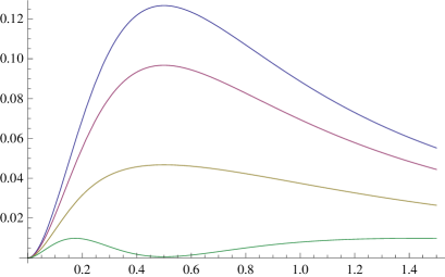
Figure 1: The density $\rho_{m}(x)$ in Example BH2 for $m=1$, $a=0.5$, and $b=0.1,\ 0.2,\ 0.3,\ 0.369$ (upside down).

The expressions for $\rho_{e}$ and $J$ turn out to be very bulky and will not be reproduced here. It is only important that, for a generic choice of $P(\chi)$, they are everywhere finite and regular and behave at the horizon as described in the previous section.

VII.2 Quasi-black holes

Example QBH1. Let us modify the BH ansatz (68) by putting

$${\,\rm e}^{2\gamma}\equiv A(x)=\frac{z^{2}}{(m+z)^{2}},\hskip 28.45274ptz:=\sqrt{x^{2}+c^{2}},$$ (75)

where $m>0,\ c>0$ are constants, and $c=0$ returns us to the case (68). At large $x$ (75) leads to $A\approx 1-2m/x+3m^{2}/x^{2}+...$, hence $m$ has again the meaning of a Schwarzschild mass. Near the center $x=0$ we have

$$A(x)=\frac{c^{2}}{(m+c)^{2}}+\frac{mx^{2}}{(m+c)^{3}}+\ldots,$$ (76)

which confirms that the center is regular and also that with $m>0$, according to (43) and (45), the matter density is positive at small $x$.

Now, calculating the first three ($\gamma$-dependent) terms in (41), we obtain

$$4\pi\rho_{m}=\frac{3mc^{2}}{z^{2}(m+z)^{3}}-\frac{z^{2}}{(m+z)^{2}}\varepsilon\chi^{\prime}{}^{2}.$$ (77)

According to (77), no phantom scalar field is needed now to provide a positive matter density, and the simplest model can be built without scalars, in the Majumdar-Papapetrou framework. Indeed, consider the ansatz (75) along with $\chi^{\prime}=0$ and $P\equiv 1$. Then $\rho_{m}$ is given by the first term in (77), Eq. (37) leads, as expected, to $\rho_{e}=\pm\rho_{m}$, and (40) to $J\equiv 0$. The total charge is then equal to mass.

To obtain a good example with the ansatz (75) but $\chi\neq{\rm const}$, let us choose $\chi^{\prime}(x)$ in such a way as to provide regularity at $x=0$ (thus $\chi^{\prime}\to 0$ as $x\to 0$) and positivity of matter density under the condition $\varepsilon=+1$. Since the first term in (77) behaves as $x^{-5}$ at large $x$, the same (or quicker) decay is required from the second term, that is, if $\chi^{\prime}\sim x^{-n}$, then $n\geq 5/2$. For example, we can take

$$\chi^{\prime}(x)=b^{2}x/z^{4},$$ (78)

with a sufficiently small constant $b>0$. It is easy to verify that $\rho_{m}>0$ at all $x$ if we take $b\leq c<m$. A point of interest is that while in the BH case ($c=0$) only a phantom scalar $\chi$ can be compatible with $\rho_{m}>0$, in the QBH case a canonical scalar ($\varepsilon=1$) is also admitted.

The expressions for $\rho_{e}$ and $J$ for any $P(\chi)$ again turn out to be cumbersome and are not presented here.

Example QBH2. Now we modify the expression (73) for $\gamma$ and put

$${\,\rm e}^{\gamma}=\frac{z}{m+2z-y},\hskip 28.45274pty:=\sqrt{x^{2}+a^{2}},\hskip 28.45274ptz:=\sqrt{x^{2}+c^{2}},$$ (79)

with certain positive constants $m,\ a,\ c$. At small and large $x$ we have

$$x\to 0: {\,\rm e}^{2\gamma}=\frac{c^{2}}{(m-a+2c)^{2}}+x^{2}\,\frac{m-a+c^{2}/a}{(m-a+2c)^{3}}+O(x^{4}),$$ (80)

$${}x\to\infty: {\,\rm e}^{2\gamma}=1-\frac{2m}{x}+\frac{3m^{2}+a^{2}-c^{2}}{x^{2}}+O(x^{-3}).$$ (81)

Such asymptotic behaviors mean that the configuration has a regular center and is asymptotically flat; as before, $m$ has the meaning of the Schwarzschild mass. Moreover, assuming

$$c<a<m,$$ (82)

we can be sure that $\rho_{m}>0$ near the center since ${\,\rm e}^{\gamma}$ has a minimum there (see Section 6). For $\rho_{m}$ we then obtain

$${}\rho_{m}=\frac{1}{y^{3}z^{2}(m-y+2z)^{4}}\Big{[}3a^{4}c^{2}(-2m+y-2z)$$

$${}\hskip 28.45274pt+c^{2}x^{2}[3m^{2}y+x^{2}(y-2z)+2c^{2}(m-y+2z)+m(-4x^{2}+6yz)]$$

$${}\hskip 28.45274pt+a^{2}\{(x^{4}+3c^{4})(m-y+2z)+c^{2}[3m^{2}y+2x^{2}(y-2z)+m(-8x^{2}+6yz)]\}\Big{]}$$

$${}\hskip 28.45274pt+\frac{\varepsilon z^{2}}{(m+2z-y)^{2}}\chi^{\prime}{}^{2}.$$ (83)

Numerical calculations show that $\rho_{m}>0$ for proper choices of the dilaton field profile $\chi(x)$ with $\varepsilon=+1$ under the same condition (82) for the model parameters.

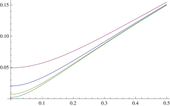
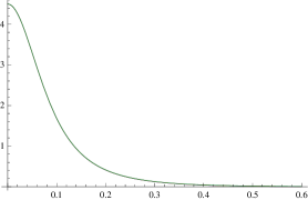
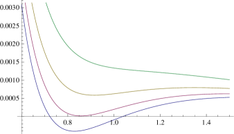
Figure 2: Plots for Example QBH2. Left: the metric function ${\,\rm e}^{2\gamma(x)}$ for $m=1$, $a=0.5$ and $c=0.025,\ 0.5,\ 0.1,\ 0.2$ (bottom-up). Middle: the density $\rho_{m}(x)$ at small $x$ for $m=1$, $a=0.5$, $c=0.1$ and $b$ ranging from 0.3 to 0.4: the $b$ dependence is indistinguishable. Right: the same for $b=0.39,\ 0.395,\ 0.398,\ 0.4$ at larger values of $x$ where the $b$ dependence is significant (upside down).

For instance, we can assume, as in (73),

$$\chi^{\prime}=b/y^{2},\hskip 28.45274ptb={\rm const}>0$$ (84)

with sufficiently small $b$. Examples of the behaviors of ${\,\rm e}^{2\gamma}$ and $\rho_{m}$ close enough to the center for certain model parameters are presented in Fig. 2. The left plot illustrates the proximity of ${\,\rm e}^{2\gamma}$ to zero near the center. The right plot makes it clear that, with the chosen values of $m,\,a,\,c$, we obtain $\rho_{m}>0$ if $b<b_{0}\approx 0.398$.

The expressions for the electric and scalar charge densities are again too large to be reproduced here; it is important that they are finite and regular, but their particular form can add nothing to our understanding of the situation.

VIII Cylindrical symmetry

Besides starlike structures described as spherically symmetric configurations, of certain interest can be stringlike ones well described in the framework of cylindrical symmetry. The corresponding static metric of the form (12) reads

$$ds^{2}={\,\rm e}^{2\gamma}dt^{2}-{\,\rm e}^{-2\gamma}(dx^{2}+dz^{2}+x^{2}d\varphi^{2}),$$ (85)

where $z\in{\mathbb{R}}$ and $\varphi\in[0,2\pi)$ are the longitudial and azimuthal coordinates. All unknowns are functions of $x$. The field equations are similar to (36)–(40):

$$2\varepsilon x^{-1}{\,\rm e}^{2\gamma}(x\chi^{\prime})^{\prime}+P_{\chi}\phi^{\prime}{}^{2} = -8\pi J(x),$$ (86)

$$x^{-1}\big{(}P{\,\rm e}^{-2\gamma}x\phi^{\prime}\big{)}^{\prime} = 4\pi\rho_{e}{\,\rm e}^{-3\gamma},$$ (87)

$$x^{-1}{\,\rm e}^{2\gamma}(x\gamma^{\prime})^{\prime}-P\phi^{\prime}{}^{2} = 4\pi\rho_{m},$$ (88)

$$\gamma^{\prime}{}^{2}+\varepsilon\chi^{\prime}{}^{2} = {\,\rm e}^{-2\gamma}P\phi^{\prime}{}^{2},$$ (89)

$$\rho_{m}\gamma^{\prime}-\rho_{e}\phi^{\prime}{\,\rm e}^{-\gamma} = J\chi^{\prime},$$ (90)

the only change is that $x^{2}$ is replaced by $x$ at some places; instead of (41) we obtain

$$4\pi\rho_{m}={\,\rm e}^{2\gamma}(\gamma^{\prime\prime}+\gamma^{\prime}/x-\gamma^{\prime}{}^{2}-\varepsilon\chi^{\prime}{}^{2}).$$ (91)

These small changes in the equations, however, drastically affect the resulting physical picture. The main features of possible nonsingular cylindrical solutions can be described as follows.

A regular axis is obtained in the metric (35) at $x=0$ if and only if at small $x$

$$\gamma(x)=\gamma_{a}+O(x^{2}),\hskip 28.45274pt\gamma_{a}={\rm const}.$$ (92)

As near a regular center, we can use the Taylor expansion (43), and it again follows that $\rho_{m}>0$ near the axis as long as $g_{00}=A(x)$ has a minimum there.

Horizons. A horizon at a finite cylindrical radius $r=x{\,\rm e}^{-\gamma}$ can exist at $x=0$ and, as in spherically symmetric systems, it is necessarily extremal (double). However, its geometry, being regular, is still quite peculiar: the longitudinal metric coefficient $g_{zz}$ blows up there, so the horizon area is infinite, just as it happens in the so-called cold black holes cold; cold-q .

Using the same Taylor expansion (46) as before, with $A_{2}>0$, we now obtain quite a different result for matter density near the horizon (assuming a finite value of $\chi^{\prime}(0)$):

$$4\pi\rho_{m}=-\sqrt{2/A_{2}}+O(x^{2}).$$ (93)

Thus the mass density is always negative at a horizon. It is a general result for cylindrical systems in our framework.

Asymptotic flatness. This property, though desirable if a stringlike configuration should be observable in our Universe, is rather rare in solutions to the field equations (recall that even the Levy-Civita well-known vacuum solution is asymptotically flat only in the trivial case where it is simply flat). For an asymptotically flat configuration with the metric (85) one can require, without loss of generality, ${\,\rm e}^{\gamma}\to 1$ as $x\to\infty$. Furthermore, if we assume, at large $x$, ${\,\rm e}^{\gamma}\approx 1+ax^{-n}$ with certain constants $a$ and $n>0$, calculating the first three terms in (91), we find that they make a positive contribution to $\rho_{m}$ (which is necessary for having a phantom-free configuration) if and only if $a>0$.

Now, suppose we have a regular asymptotically flat configuration (e.g., something like a QBH) with a regular axis. Then, at large $x$ the function $A(x)=e^{2\gamma}$ is decreasing whereas at $x=0$ it has a minimum. It means that $A(x)$ necessarily has a maximum at some finite $x=x_{0}$. Putting in its neighborhood $A=A_{0}+{{\textstyle\frac{1}{2}}}A_{2}(x-x_{0})^{2}+\ldots$, with $A_{2}<0$ to provide a maximum, and substituting this expansion to (91), we obtain that the first three terms in (91) contribute negatively to $\rho_{m}$ near $x_{0}$, so that $\rho_{m}>0$ can be obtained only with $\varepsilon=-1$.

We conclude that neither cylindrical BHs nor stringlike DMP configurations with a regular axis (in particular, stringlike QBHs) can be phantom-free. Therefore we abstain from giving particular examples here.

IX Conclusion

The well-known static MP systems in GR include gravitational and electromagnetic fields and electrically charged dust with equal densities $\rho_{m}=|\rho_{e}|$. We have considered a generalization of MP systems, including a dilatonic scalar field (the dilatonic MP, or DMP systems) with an arbitrary coupling function $P(\chi)$ in the Lagrangian (1), where the scalar field $\chi$ may be normal or phantom. As in MP systems, the metric has a conformally flat spatial part. A DMP system is characterized by the metric function $\gamma(x^{i})$, the electric potential $\varphi(x^{i})$, the dilaton field $\chi(x^{i})$, and three densities, those of mass, $\rho_{m}(x^{i})$, electric charge, $\rho_{e}(x^{i})$, and scalar charge, $J(x^{i})$. Let us enumerate the main results obtained.

1. It has been shown that static configurations are possible with arbitrary functions $g_{00}={\,\rm e}^{2\gamma(x^{i})}$ ($i=1,2,3$) and $\chi=\chi(\gamma)$, for any regular coupling function $P(\chi)$, without any assumption of spatial symmetry.

2. For general static systems, the field equations imply that the functions $\gamma(x^{i})$, $\chi(x^{i})$ and $\phi(x^{i})$ are related, so that if, say, $\gamma(x^{i})\neq{\rm const}$, then $\chi=\chi(\gamma)$ and $\phi=\phi(\gamma)$. It is thus unnecessary to postulate the existence of such functional relations, as is often done.

3. There are purely scalar analogs of MP systems, but only with phantom scalar fields. However, the corresponding point sources are different: an extreme BH for MP, a singularity for scalar MP.

4. It has been shown that sufficiently general configurations with nontrivial scalar fields cannot be obtained without a nonzero scalar charge density $J$; this, however, does not forbid the existence of special solutions with $J\equiv 0$ for particular $P(\chi)$.

5. There is a universal balance condition, (53), between the Schwarzschild mass and the electric and scalar charges, valid for any asymptotically flat DMP systems, including those with horizons and/or singularities. It generalizes the results previously obtained for special cases (see, e.g., clem2 ).

6. In the case of spherical symmetry, the existence conditions have been formulated for BH and quasi-BH (QBH) configurations with smooth matter, electric charge and scalar charge density distributions. It turns out that horizons in DMP systems are second-order (extremal), in agreement with the general properties of QBHs lemos4 .

7. For QBHs containing a small parameter $c$ whose nonzero value distinguishes them from BHs, different limiting transitions $c\to 0$ are analyzed. They lead to universal solutions independent of the particular choice of a QBH configuration. The limiting metrics coincide with those obtained previously for MP systems.

8. Examples of spherically symmetric BH and QBH solutions have been obtained. Among them are phantom-free ones, that is, the mass density and the energy densities of both scalar and electromagnetic fields are nonnegative.

9. For cylindrically symmetric configurations, the conditions at a regular center, a possible horizon and at flat infinity have been formulated. It has been shown that neither cylindrical BHs nor stringlike DMP configurations with a regular axis (in particular, stringlike QBHs) can be phantom-free.

Some of these results have been briefly presented in we-14 , viz., items 1, 3, 5, and 8 (partly). In addition, in we-14 , polycentric configurations, possible in the DMP framework, were discussed, with any number of mass concentrations. For instance, one can consider the metric (12) in Cartesian coordinates $x^{i}=(x,y,z)$ (so that $h_{ik}=\delta_{ik}$) and choose

$${\,\rm e}^{-\gamma(x^{i})}\equiv f(x^{i})=\frac{1}{n}\sum_{a=1}^{n}f_{a}(X_{a}),$$ (94)

where $f_{a}$ are functions of $X_{a}:=|x^{i}-x^{i}_{a}|$, $x^{i}_{a}$ being the (fixed) coordinates of the $a$-th center. As $f_{a}$, one can take any functions providing asymptotically flat spherically symmetric solutions, e.g., BHs or QBHs. A complete solution is obtained after choosing the function $\chi(\gamma)$, or equivalently $\chi(f)$, which should be regular at all relevant values of $f$ and decay sufficiently rapidly at spatial infinity, as $f\to 1$. In we-14 , an example is given of such a system with two mass concentrations, where each “center” can be a BH or a QBH.

We would like to stress that it is in general rather difficult to find sources that admit QBH configurations since matter begins to collapse long before approaching a would-be horizon. It is the freedom in choosing the metric function $\gamma(x)$ that enables us to keep DMP configurations static even extremely closely to emergence of a horizon.

Acknowledgments

We thank CNPq (Brazil) and FAPES (Brazil) for partial financial support.

References

- (1) S.W. Hawking and G.F.R. Ellis, The Large Scale Structure of Space-Time (Cambridge University Press, Cambridge, 1973).
- (2) V.P. Frolov and I.D. Novikov, Black Hole Physics. Basic Concepts and New Developments (Kluwer, 1997).
- (3) S.D. Majumdar, Phys. Rev. 72, 390 (1947).
- (4) A. Papapetrou, Proc. Roy. Irish Acad. A51, 191 (1947).
- (5) José P.S. Lemos and E.J. Weinberg, Phys. Rev. D 69, 104004 (2004).
- (6) José P.S. Lemos and O.B. Zaslavskii, Phys. Rev. D 76, 084030 (2007).
- (7) José P.S. Lemos and O.B. Zaslavskii, Phys. Rev. D 82, 024029 (2010).
- (8) José P.S. Lemos and O.B. Zaslavskii, Phys. Lett. B 695, 37 (2011).
- (9) José P.S. Lemos, Scientific Proceedings of Kazan State University (Uchonye Zapiski Kazanskogo Universiteta (UZKGU)) 153, 215 (2011); arXiv: 1112.5763.
- (10) W.B. Bonnor, Class. Quantum Grav. 16, 4125 (1999).
- (11) W.B. Bonnor, Gen. Rel. Grav. 42, 1825 (2010).
- (12) R. Meinel and M. Hütten, Class. Quantum Grav. 28, 225010 (2011).
- (13) I.Z. Fisher, Zh. Eksp. Teor. Fiz. 18, 636 (1948); gr-qc/9911008.
- (14) O. Bergmann and R. Leipnik, Phys. Rev. 107, 1157 (1957).
- (15) K.A. Bronnikov, Acta Phys. Pol. B4, 251 (1973).
- (16) N.M. Bocharova, K.A. Bronnikov and V.N. Melnikov, Vestnik MGU, Fiz., Astron., No.6, 706 (1970).
- (17) C. Brans and R.H. Dicke, Phys. Rev. 124, 925 (1961).
- (18) K.A. Bronnikov, G. Clément, C.P. Constantinidis and J.C. Fabris, Phys. Lett. A243, 121 (1998), gr-qc/9801050.
- (19) K.A. Bronnikov, G. Clément, C.P. Constantinidis and J.C. Fabris, Grav. Cosmol. 4, 128 (1998), gr-qc/9804064.
- (20) K.A. Bronnikov, C.P. Constantinidis, R.L. Evangelista and J.C. Fabris. Int. J. Mod. Phys. D 8, 481 (1999); gr-qc/9902050.
- (21) T. Damour and A.M. Polyakov, Nucl. Phys. B 423, 532–558 (1994); hep-th/9401069.
- (22) T. Damour and A.M. Polyakov, Gen. Rel. Grav. 26, 1171–1176 (1994); gr-qc/9411069.
- (23) K.A. Bronnikov and G.N. Shikin, Izvestiya Vuzov SSSR, Fiz., No. 9, 25 (1977).
- (24) K.A. Bronnikov and G.N. Shikin, Russ. Phys. J. 20 (9), 1138–1143 (1977).
- (25) G. W. Gibbons and K. Maeda, Nucl. Phys. B 298, 741 (1988).
- (26) D. Garfinkle, G.T. Horowitz, and A. Strominger, Phys. Rev. D 43, 3140 (1991); Erratum: Phys. Rev. D 45, 3888 (1992).
- (27) M. Rakhmanov, Phys. Rev. D 50, 5155 (1994)
- (28) K.A. Bronnikov, V.N. Melnikov, and G.N. Shikin, Izvestiya Vuzov SSSR, Fiz., No. 11, 69 (1978).
- (29) K.A. Bronnikov, V.N. Melnikov, and G.N. Shikin, Russ. Phys. J. 21 (11), 1443 (1978).
- (30) K.A. Bronnikov, V.N. Melnikov, G.N. Shikin, and K.P. Staniukovich, Ann. Phys. (NY) 118 (1), 84 (1979).
- (31) V.D. Ivashchuk and V.N. Melnikov, Class. Quantum Grav. 14, 3001 (1997); Corrigendum ibid. 15, 3941 (1998); hep-th/9705036.
- (32) V.D. Ivashchuk and V. N. Melnikov, Class. Quantum Grav. 18, R87–R152 (2001); hep-th/0110274.
- (33) K.A. Bronnikov, Grav. Cosmol. 1, 67–78 (1995).
- (34) K.A. Bronnikov, V.D. Ivashchuk and V.N. Melnikov, Grav. Cosmol. 3, 203–212 (1997).
- (35) K.A. Bronnikov, Grav. Cosmol. 4, 49–56 (1998); hep-th/9710207.
- (36) V.D. Ivashchuk and V. N. Melnikov, Grav. Cosmol. 17, 328–334 (2011).
- (37) G. Clément, J.C. Fabris, and M.E. Rodrigues, Phys. Rev. D 79, 064021 (2009).
- (38) M. Azreg-Ainou, G. Clément, J.C. Fabris, and M.E. Rodrigues, Phys. Rev. D 83, 124001 (2011); arXiv: 1102.4093.
- (39) S. Yazadjiev, Mod. Phys. Lett. A 20, 821 (2005); arXiv: gr-qc/0411132.
- (40) K.A. Bronnikov, J.C. Fabris, R. Silveira, and O.B. Zaslavskii, Phys. Rev. D 89, 107501 (2014); ArXiv: 1405.6116.
- (41) K.A. Bronnikov and S.G. Rubin, Black Holes, Cosmology, and Extra Dimensions (World Scientific, 2012).
- (42) R. Geroch, Commun. Math. Phys. 13, 180 (1969).
- (43) B. Bertotti, Phys. Rev. 116, 1331 (1959).
- (44) I. Robinson, Bull. Acad. Pol. Sci. 7, 351 (1959).
- (45) F.G. Alvarenga, A.B. Batista, J.C. Fabris, and G.T. Marques, Phys. Lett. A 320, 83 (2003).
- (46) F.G. Alvarenga, A.B. Batista, J.C. Fabris, and G.T. Marques, Grav. Cosmol. 10, 184 (2004).