Universidad Autónoma de Madrid
Facultad de Ciencias
Departamento de Física Teórica
The flavour of supersymmetry:
Phenomenological implications
of sfermion mixing
Memoria de Tesis Doctoral realizada por

Miguel Arana Catania
presentada ante el Departamento de Física Teórica

de la Universidad Autónoma de Madrid

Trabajo dirigido por la

Dra. María José Herrero Solans,

Catedrática del Departamento de Física Teórica

y miembro del Instituto de Física Teórica, IFT-UAM/CSIC

y por el

Dr. Sven Heinemeyer,

Investigador científico del Instituto de Física de Cantabria IFCA (CSIC-UC)

Madrid, diciembre de 2013

  

  

  

Agradecimientos

Este capítulo es uno de los más importantes de esta tesis. No trata sobre ciencia, sino sobre el mundo que hay ahí fuera mientras hacemos ciencia. Ese mundo debería saltar por los aires en un millón de pedazos a cada segundo, y sin embargo hay gente, hay formas de vivirlo, que permiten que siga girando, que mantenga el calor, que al acabar un día empiece otro. Ante eso no hay nada que decir, sólo inclinarse y agradecer, profundamente:

a mi madre, mi padre, mi hermano y mis hermanas, sus parejas, y mis sobrinas, por ese amor que me ha arropado siempre, con un calor total e impenetrable, y que ha estado por encima de todo; por ese hogar tan único, tan privilegiado, desde el que salir al mundo, por hacer de lo elevado la normalidad, por esa visión profunda y completa del mundo con la que poder orientarme, por comprender siempre tan claramente lo que importa, por los pasos que seguir e imitar con profundo orgullo, desde aquí o desde el recuerdo de otros, por hacerlo todo fácil, y enseñarme que no tiene por qué ser de otra manera.

a Adrián, Ángel, Antonio, Mar, Ana, Victor, María, Sandra, Sergio y Álvaro, por haber estado ahí desde siempre, tan mezclados y diferentes, por ser un refugio frente a lo de fuera, por las costumbres, los roles, lo eternamente repetido que hace el hogar.

a Germán, Irene, Victor, Arianna, Edoardo y otros compañeros de laboratorio que hemos vivido juntos esa nueva extraña madurez de pasar a ser profesores. Me alegro mucho de que haya sido con vosotros ese momento único.

a María, Juan y Sofía, por haberme abierto el camino a, y compartido, esa locura, esa obsesión; porque encontrarse bajo los focos es encontrarse en una parte muy única del mundo, eso ya no se nos va a pasar; por el cariño, por las risas, por las millones de horas unos con otros, muy cerca.

a María José, por estos años compartiendo la investigación, por enseñarme todas estas cosas, por darte tanto en lo que haces, por la cercanía, por crear todos esos momentos buenos y divertidos, que han sido muchos. Sobre los malos momentos, espero que te libres de esa incapacidad para permitir las formas de hacer las cosas de los otros, vas a hacer que la gente sea más feliz a tu alrededor.

a Sven, por hacer ciencia conmigo, por enseñarme a hacerla, por la sonrisa infatigable (en un sentido totalmente literal), por no poner barreras, por estar siempre preparado para soltar una carcajada, por las noches de cervezas, por cada momento divertido y cercano, también excepcionalmente numerosos.

a Juanjo, por pensar a lo grande siempre, por pensar diferente, y pensar conmigo; por enseñarme, por esas noches tremendas, por las que vendrán.

a todos los profesores que he tenido desde el colegio hasta la universidad que han querido enseñar, especialmente a los que han sabido encontrar el verdadero conocimiento oculto entre montañas de enseñanzas prescindibles; a los que han sido capaces de volver a las aulas día tras día, año tras año, sin perder la felicidad y la fuerza.

a Andrea, mi bichillo, por haberme querido tanto, por querer compartir toda tu vida, esa tan única, por haber hecho mi vida mejor, más importante, por haberme dado tantas risas, por esa energía inagotable que lo cambia todo.

a Ernesto, por confiar, por dejarme jugar, por dejarme crecer. Y por bella persona. Muy bella.

a todos los que contribuyen de alguna manera a que exista la universidad y la investigación pública. Que nos permiten que podamos dedicar los días de nuestra vida a esto tan fascinante. A los que entienden la importancia absoluta de la tarea.

a Javi por esa mirada siempre limpia, siempre abierta sobre el mundo, tan poco usual; por llevarla con la total certeza de que así el mundo es mejor, y a pesar de todos esos hombres grises obsesionados porque seas uno de ellos; por salir victorioso tantas veces de la lucha contra tu parte oscura, por todos los grandes juegos que hemos vivido juntos, en la física, en la política, en el mundo,… qué divertido.

a los que no se resignan a un mundo gris y mediocre donde la vida no importe; a los que exigen belleza, a los que exigen felicidad.

a mis compas de la casa de las flores y de tantas vueltas por el mundo (también Jules, Etor y Susana!), por hacer allí y aquí fáciles y divertidos los miles de minutos que tiene cada día, que es tan fundamental. Those are for you.

a Álvaro, por todo, aunque a veces se haga complicado.

a Jorge Alemán, por ayudarme con esa otra investigación tan complicada, con tanta energía y dedicación, poniendo en ella toda esa cabeza tan genial.

a Ana, porque hemos sobrevivido a la gran guerra, y ahora desde la residencia para veteranos tullidos y borderline podemos contar batallitas; por la absurdidad, por esa risa ultradecibélica, por eso que hace que todos se arremolinen siempre a tu alrededor (incluso aunque intentemos escapar). Hubiera sido tan aburrido sin ti!

a los que buscan trascender esta realidad.

a Alice y Daniel, por hacerme querer una y otra vez parar todo para simplemente estar con vosotros, porque en esa casa no se paren de escuchar risas.

a toda la gente que salió a las plazas, que con naturalidad fue a encontrarse y a iniciar una revolución; que le dieron la espalda al supuesto poder, para hablar y pensar juntos durante 1001 noches lo que debía ser el mundo; que callaron a tertulianos, analistas, falsos, manipuladores, demagogos y cobardes, y demostraron quiénes somos realmente

a Helen, por ese tiempo de cuento.

a Siannah y Arian, por ese carácter siempre tranquilo, esa disposición amable, que hace tan agradable investigar y estar con vosotros.

a los que comparten cultura, software y conocimiento en internet, y ayudan a acabar con el concepto de “propiedad intelectual”, porque mi vida ha sido tremendamente más rica gracias a ello.

a todos mis compañeros de despacho por convertir un espacio de trabajo muerto en un lugar de convivencia donde querer volver. Nos pasamos la mayor parte de nuestra vida ahí, no es algo menor, es muy importante.

a Javier Menéndez (und África natürlich) por dejarme, divertido y tranquilo como siempre eres, tomar el despacho y armar ruido y radionovelas; porque para un doctorando novato es fundamental tener modelos por encima de uno de los que aprender, y yo he tenido mucha suerte en esto.

a Steve Blanchet, que trajo la belleza y la elegancia al despacho, por hacernos un hueco tan cálido y cercano en tu vida, por querer compartir con nosotros tantas risas explosivas (sobre todo cuando podrías estar machacando a Federer).

a Liliana, que calladita calladita nos fuiste conquistando a todos. Y a Luis, por ser un show con patas (aunque no te dejes querer).

a Josu y Xabi, porque es un orgullo tener unos hermanos pequeños como vosotros, por aceptarme como hermano mayor, por traer mucho ruido y buen humor al despacho, por ser el par más único de todo el instituto.

a Sylwia, por la dulzura, por hacer el mundo fácil y feliz, y bonito, siempre, en cualquier lugar, meine schöne kleine Pferd.

a los amigos del 15M (Clara, Stéphane, Pablo, Aya, Juanlu, los compas de wet, Eric, Gregorio, Eduardo,… y cientos otros) con los que hemos vivido con pasión cómo la historia tomaba forma delante de nuestros ojos, cómo nuestras fantasías se hacían realidad; que hemos pasado las noches y los días, y cada minuto juntos, pensando mundos, trazando revoluciones, hasta que caíamos rendidos unos sobre otros.

a mi familia argentina: los Larriera, Silvia, Memé, Renée, Miguel, Luly, Darío, Amanda, Maruja, Rodo, Ana, Justo, Mennella, los Regueiro (que ya estáis bastante argentinizados), Alejandro, Nory, Liliana, Vilma, Diana y Cacho, por el calor familiar que no ha faltado nunca, por la mitad de mi educación que han sido esas comidas familiares en casa, por crecer rodeado de la risa y la palabra.

a todos los que emplean el tiempo de sus vidas en cambiar el mundo, en que los demás vivan mejor. A los que para hacerlo tienen que buscar grietas en sus vidas y trabajos por donde escaparse.

a Ángel, nuestro filósofo, por el humor siempre presente a pesar de la conciencia de la tragedia, por la entrega incondicional a tus amigos, por guiar, por enseñar, por ser un referente, por no querer nunca ser más que el otro, sea quien sea, por mantenerte siempre elevado, con total ligereza.

a los hypáticos, por haber convertido ese cuartucho de la facultad en el rincón más interesante y excitante de toda la universidad, por la maravillosa mezcla, por la brillantez, por la educación recibida, por los caminos que seguir, por jugarlo todo siempre en los límites, por buscar el día siguiente.

al No-grupo por habernos enamorado tan intensamente, por esas cabecitas tan geniales, por las noches de conspiración para cambiar el mundo, por cuidarnos unos a otros.

a los que fallan, a los que no llegan, a los que no son capaces.

a Mario Sanz, por el cariño, la cercanía, la sensibilidad, por compartir tanto, tan personal, tan especial.

a todos los científicos que ofrecen sus vidas para poder colaborar en la construcción del conocimiento humano; millones de personas que mano con mano empujan haciéndonos avanzar a todos; que llegan cada día a sus despachos y laboratorios sabiendo que la sociedad no les va a recompensar, ni agradecer; que pasarán desapercibidos, que sólo habrá silencio. Y en ese silencio se dedican a trabajar contentos.

a Álvaro pensamiento, por ser una persona de una calidad humana excepcional.

a Nadir, por sobrevivir hombro con hombro (y gracias a eso precisamente), al frío de Berlín; por lanzarte conmigo a abrir ruta tras ruta, y estar ahí siempre que se te necesita.

a Carlos, por las infinitas noches pensando universos, planeando revoluciones, disfrutando los infinitos otros mundos que vamos encontrando, pensando la estructura escondida de este; por pensar libre, sin límites ni esquemas, y lanzarte a darle vida a cualquier idea genial; por la sabiduría, por la incorruptibilidad, por la ausencia de ego, por la constante tranquilidad.

  

A todos ellos va dedicado este trabajo.

Chapter 1 Introducción

El 4 de julio de 2012 fue anunciado internacionalmente en un evento en vivo que el bosón de Higgs había sido descubierto [3, 4, 5]. En los pocos segundos que tardó la señal transmitida en viajar alrededor del mundo, la humanidad dio un enorme salto hacia adelante en nuestro conocimiento del universo. No es muy común que el avance científico cristalice en un evento tan específico, y de tal magnitud, así que los que vivimos ese momento debemos atesorarlo. ¿Qué ocurrió ese día? ¿qué clase de cambio produjo en el mundo? y después del salto ¿dónde estamos ahora?

El descubrimiento es un movimiento dialéctico de apertura y cierre. El cierre se produce con respecto al Modelo Estándar (SM) de las interacciones fundamentales, y produjo en muchos físicos un sentimiento de alivio después del anuncio. El bosón de Higgs es la última pieza que faltaba del SM, nuestro modelo actual de física de partículas desarrollado durante más de 40 años [6, 7, 8, 9, 10]. El SM es una teoría cuántica de campos renormalizable en 4 dimensiones con una simetría gauge $SU(3)_{C}\times SU(2)_{L}\times U(1)_{Y}$, invariante bajo transformaciones de Poincaré y CPT. El bosón de Higgs es la partícula que aparece como consecuencia del mecanismo de Brout-Englert-Higgs [11, 12, 13, 14, 15], necesario en el SM para dar masa a las partículas elementales. Al mismo tiempo que el SM, extendido con masas de neutrinos, ha demostrado experimento tras experimento ser capaz de coincidir en sus predicciones con cada medida que se ha podido imaginar jamás en el campo de la física de partículas de altas energías, el bosón de Higgs se ha mantenido escondido. El extraordinario éxito del modelo entraba en conflicto con la elusividad de su última predicción. Pero finalmente el descubrimiento del bosón de Higgs se ha producido en el laboratorio CERN, por los dos experimentos ATLAS [4] y CMS [5]. Estos experimentos han medido una partícula tipo Higgs con spin 0, sin cargas eléctrica o de color y paridad positiva (aunque esto último está todavía estudiándose), como predecía el SM, y con una masa entre 125 y 126 GeV [16, 17] compatible con las restricciones del polo de Landau y de la estabilidad del vacío del SM hasta energías muy altas, cercanas a la masa de Planck $M_{P}=10^{19}$GeV (el SM no predice un valor concreto de la masa del bosón de Higgs, pero pone límites superiores e inferiores al mismo; en concreto dentro del SM puro parece que vivimos en un vacío metaestable de vida larga [18, 19]). Con este descubrimiento se cierra un capítulo importante en la historia de la física de partículas. Probablemente ninguna otra construcción humana pueda ser comparada ahora en complejidad y solidez al SM. El nivel de concordancia entre las predicciones del modelo y los resultados de los experimentos alcanza por ejemplo el orden de $10^{-12}$ en la medida del momento magnético del electrón [20, 21].

Sin embargo, el SM no es una teoría final en física de partículas. Y aquí viene la apertura. Hay muchos fenómenos en el universo que el SM no es capaz de explicar, así que está claro que no es un modelo completo de la física de nuestro universo, y por lo tanto debe ser ampliado o introducido en una teoría más extensa. Por ejemplo, el SM no incluye ni la masa ni las oscilaciones de los neutrinos, a pesar de que experimentos como Super-Kamiokande hayan probado ambos hechos [22]. Tampoco incluye un candidato como partícula de materia oscura. De hecho, el bosón de Higgs está en conexión directa con el principal fenómeno que escapa a nuestro control: la masa de las partículas elementales. Aparte de esto y desde un punto de vista más general en física, con respecto a la masa gravitacional, otra de las principales preguntas abiertas sería cómo unir los niveles gravitacional y cuántico en una teoría unificada que describa todas las fuerzas en un marco común. El objetivo sería cuantizar la gravedad, si miramos el problema desde el punto de vista de la teoría cuántica de campos; una cuestión que evidentemente no está resuelta en el SM ya que la gravitación es la única interacción que no está incluída en el modelo. Sin embargo, desde la perspectiva que será más relevante para nuestro trabajo, donde nos mantendremos al nivel de la teoría cuántica de campos y las fuerzas gravitacionales serán despreciables, el problema de la masa puede ser reformulado de otra manera en lo que se conoce como el problema del sabor.

El problema del sabor, formulado a grandes rasgos, podría ser entendido como la ausencia de una teoría capaz de explicar el papel que juega la masa en nuestro modelo de física de partículas. Esto se traduce en un conjunto de características o fenómenos observados que no somos capaces de explicar. Por ejemplo, las partículas elementales aparecen como ‘familias’ de partículas, donde cada familia es una copia de la anterior en los números cuánticos, pero difiere en las masas. La existencia de estas familias y su número (3 en el SM, siendo esto totalmente compatible con los actuales límites experimentales, véase por ejemplo [23]) no tienen explicación en el SM. El patrón de las masas de las partículas también parece arbitrario, con vastas regiones vacías en la escala de masas como el espacio entre las masas de los neutrinos y del electrón, desde aproximadamente $10^{-9}$ GeV a $0.51\times 10^{-3}$ GeV, o los dos órdenes de magnitud entre la masa del quark bottom con 4.18 GeV y la masa del quark top con 173.2 GeV. Los valores de los elementos de las matrices de mezcla entre familias de fermiones, CKM [24, 25] y PMNS [26, 27, 28], tampoco son predichos por el SM. Estas y otras preguntas sobre el sabor abren una nueva ventana a la fenomenología más allá del SM que consideraremos a lo largo de este trabajo. En este sentido, entender las características del bosón de Higgs, siendo este el campo responsable de las masas de las demás partículas a través del mecanismo de Brout-Englert-Higgs, que rompe espontáneamente la simetría electrodébil $SU(2)_{L}\times U(1)_{Y}$ en la simetría electromagnética $U(1)_{em}$, puede darnos pistas para entender el problema del sabor y para buscar señales de nueva física a través de la fenomenología del bosón de Higgs y del sabor. La última pieza del ‘viejo’ modelo puede convertirse así en la primera piedra del ‘nuevo’.

El descubrimiento del bosón de Higgs abre situaciones muy prometedoras al mismo tiempo que va cerrando los capítulos del SM. Este movimiento en zigzag entre el pasado y el futuro puede verse en diferentes aspectos del descubrimiento: las interacciones entre el bosón de Higgs y el resto de partículas están siendo medidas en este momento en el LHC, y por el momento son compatibles con los valores del SM [29, 30, 31, 16, 32, 17, 33]. Sin embargo, en la próxima fase del LHC la precisión en estas medidas será ampliamente mejorada [34, 35, 36, 37] abriendo una puerta a la medida de efectos de física más allá del SM en el valor de estos acoplamientos. Por otro lado, aunque la naturaleza fundamental versus compuesta del bosón de Higgs no ha sido todavía desentrañada por los experimentos, si la hipótesis del SM de ser una partícula escalar fundamental es finalmente confirmada, esto supondrá un nuevo hito. De esta forma se dará un paso adelante en el entendimiento de teorías con escalares fundamentales en ellas, como diferentes modelos de física más allá del SM, y en particular el que consideraremos en este trabajo. Como otro movimiento, la medida de la masa del bosón de Higgs cierra la casilla vacía de la tabla de propiedades de las partículas del SM, pero abre nuevas posibilidades dado que esta masa puede estar relacionada con la escala de la nueva física, o la masa de sus nuevas partículas, todavía desconocidas, como veremos a lo largo de este trabajo. De nuevo una medida de mayor precisión, en este caso de la masa del bosón de Higgs, nos dará información sobre nueva física, ya que esta estará también relacionada con las características de los nuevos modelos de física más allá del SM.

Respecto a la nueva física, supersimetría (SUSY) [38, 39, 40] será nuestra elección como nueva simetría subyacente a la física más allá del SM, y en particular nos centraremos en el Modelo Estándar Supersimétrico Mínimo (MSSM) [41, 42, 43]. La principal idea en la base de los modelos supersimétricos es añadir una nueva simetría que relaciona bosones y fermiones, como aspectos parciales de un elemento más fundamental en la construcción del universo llamado supercampo. De nuevo se repite la idea que ha conducido gran parte de la historia de la física de encontrar constituyentes más simples que dan lugar a las múltiples entidades que nos rodean, y de nuevo la idea de un universo más simétrico bajo la apariencia del que vemos. De hecho, del teorema de Haag-Lopuszanski-Sohnius [44] sabemos que supersimetría es la única extensión no trivial del grupo de Poincaré de teorías cuánticas relativistas en 3+1 dimensiones. Esta sencilla idea de una simetría entre fermiones y bosones se convierte en un poderoso motor cuyo desarrollo ha llevado a la construcción de teorías supersimétricas en las que se resuelven diferentes problemas o aspectos poco atractivos del SM: supersimetría incluye muchas características atractivas como la unificación de las interacciones del SM, la posibilidad de resolver el problema de la materia oscura, la naturalidad de la ruptura de la simetría electrodébil o la conexión de supersimetría con una versión gauge local de la gravedad o con interesantes teorías de altas energías como teoría de cuerdas.

El MSSM es la versión supersimétrica mínima del Modelo Estándar. Supone la introducción de una nueva partícula supersimétrica compañera para cada grado de libertad del SM, con los mismos números cuánticos bajo el grupo gauge $SU(3)_{C}\times SU(2)_{L}\times U(1)_{Y}$, pero con un spin que difiere en 1/2. Por cada fermión se introducen dos sfermiones, con spin 0: dos squarks, ${\widetilde{q}_{L}}$ y ${\widetilde{q}_{R}}$, para cada quark, y dos sleptones, ${\widetilde{l}_{L}}$ y ${\widetilde{l}_{R}}$, para cada leptón. Por cada bosón gauge con spin 1 se introduce un gaugino con spin 1/2: gluinos $\widetilde{g}$, winos $\widetilde{W}^{\pm}$ y binos $\widetilde{B}^{0}$. El sector de Higgs del MSSM es diferente al del SM, con dos dobletes de Higgs en lugar de uno, y los correspondientes compañeros de spin 1/2, los Higgsinos. Esto producirá 5 bosones de Higgs físicos: dos bosones neutros $h$ y $H$ con ${\cal CP}=+1$ (siendo el primero el más ligero), un bosón neutro pseudoescalar $A$ con ${\cal CP}=-1$, y dos bosones cargados $H^{+}$ y $H^{-}$. El bosón de Higgs observado en el LHC correspondería, en la versión más plausible del MSSM, al bosón de Higgs neutro más ligero del MSSM $h$, y esta será la hipótesis que consideremos a lo largo de este trabajo. En la actualidad todas las observaciones son compatibles con un bosón de Higgs de tipo SM, pero un bosón de Higgs supersimétrico podría imitar el comportamiento del bosón del SM, así que se necesitarán medidas de alta precisión de sus propiedades para concluir finalmente si la partícula observada es supersimétrica o no. Después de la ruptura de simetría electrodébil los Higgsinos se mezclan con los winos y binos, produciendo los charginos ${\tilde{\chi}_{1,2}}^{\pm}$ (con carga eléctrica), y los neutralinos ${\tilde{\chi}_{1...4}}^{0}$ (sin carga eléctrica). El neutralino más ligero es generalmente el candidato preferido como partícula de materia oscura [45, 46].

Un modelo con supersimetría exacta implicaría que las nuevas partículas supersimétricas tendrían las mismas masas que sus compañeras conocidas del SM, y dado que no han sido vistas todavía en los experimentos, un modelo consistente necesita implementar una ruptura suave de supersimetría capaz de elevar el valor de las masas de estas spartículas por encima del alcance de los experimentos. Los límites inferiores de exclusión actuales provenientes de los datos del LHC respecto a las masas de las spartículas están situados aproximadamente a un nivel de ${\cal O}\textrm{(1 TeV)}$ [47, 48], siendo los más restrictivos aquellos para las spartículas con interacción fuerte: los gluinos y los squarks, que se predice que serán producidos más abundantemente que el resto de partículas supersimétricas. Una SUSY natural se esperaba por debajo o alrededor de la escala del TeV, siendo esta la solución del llamado problema de la jerarquía. Este problema de la jerarquía consiste en el hecho de que la masa del bosón de Higgs obtiene correcciones radiativas que crecen cuadráticamente con la escala cut-off de la teoría de alta energía, generando correcciones gigantes por ejemplo de 15 órdenes de magnitud más grandes que la masa inicial a nivel arbol para un cut-off de la escala de Planck de $10^{19}$ GeV. Por lo tanto los contratérminos deben ser ajustados con una precisión extrema para cancelar estas correcciones y producir la masa del bosón de Higgs observada. SUSY se proponía como solución al problema de la jerarquía; sin embargo la capacidad de SUSY para resolver esta cuestión se vuelve más débil según SUSY se va volviendo más pesada, y por lo tanto más rota.

La ausencia de partículas supersimétricas en el LHC vuelve crucial el estudio de sus consecuencias fenomenológicas de otras formas diferentes a las búsquedas directas. Los efectos indirectos de SUSY en los observables de precisión y en la física del sabor son formas únicas de encontrar señales indirectas de SUSY. Estas búsquedas indirectas de nuevas partículas se han usado con anterioridad en el pasado para construir el propio SM y para comprobar la existencia de quarks pesados del SM antes de su descubrimiento. Por ejemplo, una búsqueda indirecta del quark top en LEP a través de observables de precisión hizo posible constreñir el valor de su masa a un intervalo pequeño [49, 50], que fue luego utilizado en Tevatron para descubrirlo en una búsqueda directa [51, 52]. Lo mismo ocurrió con el bosón de Higgs [50, 53]. Los efectos de los quarks charm y bottom aparecieron indirectamente en la fenomenología de mesones en procesos con cambio de sabor antes de que estos quarks fueran descubiertos [54, 55, 56]. La ventana que se abre ahora para probar la física más allá del SM a través de procesos con cambio de sabor es incomparable debido a la gran supresión de procesos con cambio de sabor en el SM. Por ejemplo, en el sector leptónico, incluso introduciendo masas y mezclas de neutrinos, las tasas de procesos de Violación de Sabor Leptónico (LFV) están enormemente suprimidas porque están determinadas por los minúsculos acoplamientos de Yukawa de los leptones. Estos generan por ejemplo valores alrededor de $10^{-60}$ en el cociente de ramificación de las desintegraciones LFV del Higgs con neutrinos masivos de Dirac o alrededor de $10^{-35}-10^{-42}$ si las masas de los neutrinos están generadas a través de un mecanismo seesaw I con masas pesadas de Majorana del orden de $10^{3}-10^{6}$ GeV [57]. En principio, en la física más allá del SM los procesos con cambio de sabor podrían no estar tan suprimidos como en el SM, y por lo tanto ser detectables en los experimentos en estos espacios vacíos dejados por el SM. En concreto, en los modelos SUSY las tasas predichas de procesos con cambio de sabor son en general de hecho demasiado grandes y están en contradicción con los experimentos. Por ello se proponen generalmente nuevas simetrías de sabor que incorporan la hipótesis de Violación de Sabor Mínima (MFV) [58], donde los acoplamientos de Yukawa son los únicos generadores de los procesos con cambio de sabor. Dado que el tamaño de estos acoplamientos de Yukawa es pequeño en general, las tasas de procesos neutros de cambio de sabor son también muy pequeñas. La única excepción es el acoplamiento de Yukawa del top que es en general el que domina en estas tasas.

La búsqueda de nueva física más allá del SM a través de procesos con cambio de sabor ha sido ya hasta cierto punto exitosa en la física de partículas: el descubrimiento de las oscilaciones de neutrinos en 1998 [22], señalando cambios de sabor en el sector de los neutrinos y como consecuencia el hecho de que los neutrinos tienen masa, no estaba contemplado en el SM, y por lo tanto es una señal de física más allá del SM. El sector cargado de los leptones no ha mostrado todavía procesos con violación de sabor pero hay experimentos desarrollándose en este momento con esperanza de detectarlos [59, 60]. La violación de sabor en el sector de los quarks sí que está incorporada en el SM a través de la matriz CKM, y este fenómeno ha sido observado en diferentes observables. Es más, los experimentos de muy alta precisión como las factorías de B [60, 61] o el LHCb [62], los convierten en candidatos únicos para distinguir posibles efectos de nueva física. Incluso cuando esta nueva física no se detecte directamente, sus masas y parámetros quedarán más restringidos por estos tipos de medidas indirectas. Las instalaciones futuras como las super factorías de B [63, 64, 65], COMET [66], Mu2e [67, 68] o PRISM [69] mejorarán significativamente las medidas de los procesos con cambio de sabor, haciendo muy prometedor el futuro de las búsquedas de violación de sabor.

Nuestro objetivo en esta tesis es describir los procesos con cambio de sabor en teorías supersimétricas con un enfoque lo más general que sea posible. Por ello utilizaremos una parametrización genérica de la mezcla de sabor en el sector sfermiónico a través de un conjunto de parámetros sin dimensión $\delta^{XY}_{ij}$ (con $X,Y=L,R$ haciendo referencia a las quiralidades de los compañeros fermiónicos; e $i$ y $j$ siendo las generaciones implicadas en la mezcla) y estudiaremos sus implicaciones fenomenológicas. Por lo tanto no nos limitaremos a la hipótesis de MFV sino que estudiaremos las implicaciones fenomenológicas del caso más general de Violación de Sabor No Mínima (NMFV). A diferencia de otros trabajos en este tema, nuestro estudio no dependerá de aproximaciones para introducir la mezcla de sabor sfermiónico, como la Aproximación de Inserción de Masa (MIA) [70], sino que realizaremos una diagonalización completa de las matrices de masa de los sfermiones con términos generales de mezcla de sabor. Este estudio nos permitirá entender en detalle las consecuencias fenomenológicas de la mezcla general de sabor sfermiónico incluso antes de descubrir los sfermiones en los experimentos.

A través de este trabajo estudiaremos diferentes observables con cambio de sabor y exploraremos sus predicciones en SUSY intentando entender sus comportamientos y consecuencias al variar los diferentes parámetros de mezcla sfermiónicos $\delta^{XY}_{ij}$, así como los parámetros del MSSM. Esto nos permitirá trazar un mapa del espacio de parámetros de mezcla de sabor sfermiónico de SUSY, conociendo qué regiones están permitidas y cuáles no, y también nos permitirá encontrar las mejores ventanas experimentales a través de la cuales buscar efectos indirectos de SUSY.

Comenzaremos nuestro estudio de la mezcla de sfermiones centrándonos en diferentes observables con cambio de sabor en el sector fermiónico. En primer lugar en el sector de los quarks, estudiaremos el cociente de ramificación de la desintegración radiativa de $B$, ${\rm BR}(B\to X_{s}\gamma)$, el cociente de ramificación de la desintegración muónica de $B_{s}$, ${\rm BR}(B_{s}\to\mu^{+}\mu^{-})$, y la diferencia de masas $B_{s}-{\bar{B}_{s}}$, $\Delta M_{B_{s}}$. En segundo lugar en el sector leptónico nos centraremos en desintegraciones como las desintegraciones radiativas $l_{j}\to l_{i}\gamma$, las desintegraciones leptónicas $l_{j}\to 3l_{i}$ y las desintegraciones semileptónicas $\tau\to\mu\eta$ y $\tau\to e\eta$. También consideraremos las tasas de conversión LFV de muones en electrones en núcleos pesados. Una vez que esto esté hecho, y conociendo las áreas permitidas para los parámetros de sabor de los sfermiones, esta tarea se completará centrándonos en los observables del bosón de Higgs, con un estudio detallado de las correcciones de masa del bosón de Higgs inducidas por mezcla de sabor de squarks. Finalmente estudiaremos las desintegraciones con violación de sabor leptónico del Higgs $\phi\to\tau\mu$ y $\phi\to\tau e$ (donde $\phi=h,H,A$) inducidos por mezclas de sabor sleptónico, dentro de las regiones permitidas por las búsquedas de LFV más restrictivas en este momento.

Durante el estudio de las desintegraciones del bosón de Higgs prestaremos especial atención al comportamiento de estos observables cuando la escala SUSY se vuelve muy pesada. La ausencia de efectos de SUSY en los experimentos puede ser entendida como consecuencia de una SUSY de una escala muy alta, donde generalmente los efectos de la nueva física desacoplan y son difíciles de ser encontrados en las observaciones. Pero como demostraremos en esta tesis, algunos observables como las desintegraciones LFV del Higgs tienen un comportamiento no desacoplante con SUSY pesada y pueden manifestarse en señales indirectas de SUSY incluso si esta SUSY pesada no aparece directamente. Tener observables no desacoplantes puede ser vital a la hora de probar SUSY, así que parte de nuestra investigación se centrará en este importante tema.

Como vemos, el descubrimiento del bosón de Higgs no señala ningún punto final. Con el cierre del SM nos embarcamos en la búsqueda abierta de supersimetría y las respuestas al problema del sabor, ya que nuestra sed de entendimiento de la realidad parece no estar satisfecha nunca. Será un nuevo viaje emocionante.

Esta tesis está estructurada como sigue: el Capítulo 3 está dedicado a resumir los aspectos más relevantes de supersimetría. Después se introduce el modelo con el que trabajaremos, el MSSM, detallando los diferentes sectores de spartículas. El Capítulo 4 resume los aspectos principales del sabor.

En el Capítulo 5 presentamos la parametrización general de sabor sfermiónico que será utilizada a lo largo del resto del trabajo, para describir la fenomenología relevante de los procesos con cambio de sabor más allá de la hipótesis de MFV. Se muestra cómo estos escenarios nos permitirán tratar con la mezcla de sabor en supersimetría de una manera general. Después de esto, presentamos los diferentes conjuntos de escenarios con los que trabajaremos aquí, con diferentes tipos de hipótesis y libertad en la elección de parámetros. Estos escenarios van desde escenarios motivados desde alta energía, definidos en el marco de supergravedad mínima, hasta escenarios de baja energía más enfocados en los actuales experimentos como los escenarios del MSSM fenomenológico.

Los siguientes cuatro capítulos recogen el núcleo de nuestra investigación y los resultados principales de esta tesis. El Capítulo 6 cubre el estudio de los efectos de mezcla de squarks en los observables de física de $B$ mencionados anteriormente. Se realiza un estudio numérico en estos observables de $B$, para obtener límites en los parámetros de sabor de los squarks.

Después de conocer las áreas permitidas en el espacio de mezcla de sabor de los squarks, entramos en el estudio de las correcciones a la masa del bosón de Higgs por mezcla de sabor de squarks en el Capítulo 7. Primero realizamos un estudio analítico de las correcciones de masa y derivamos las fórmulas a un loop necesarias. Después de esto, usamos esas fórmulas para estudiar los efectos en las masas de los bosones de Higgs de los parámetros permitidos de mezcla de sabor de los squarks.

En el Capítulo 8 estudiamos las consecuencias de la mezcla de sfermiones en el sector sleptónico. En este capítulo estudiamos los procesos más relevantes con cambio de sabor en el sector leptónico incluyendo desintegraciones radiativas $l_{j}\to l_{i}\gamma$, desintegraciones leptónicas $l_{j}\to 3l_{i}$, las desintegraciones semileptónicas $\tau\to\mu\eta$ y $\tau\to e\eta$ y la conversión $\mu-e$ en núcleos, y extraemos de ellos los observables más restrictivos que imponen los principales límites a los parámetros de mezcla de sabor sleptónico.

El Capítulo 9 concluye el estudio de las consecuencias fenomenológicas de la mezcla de sleptones con un estudio de las desintegraciones LFV de bosones de Higgs. Estas desintegraciones se estudian comparándolas con los observables LFV más restrictivos estudiados anteriormente, para encontrar las ventanas experimentales más interesantes para probar indirectamente SUSY. Se presta especial atención al comportamiento desacoplante/no desacoplante con SUSY pesada de estos observables, que será de gran interés en un futuro cercano ya que el no tener por el momento ninguna señal de SUSY sitúa las partículas supersimétricas en la región pesada por encima de la escala del TeV.

Esta tesis se concluye con el Capítulo 10, donde se recogen las conclusiones generales derivadas de este trabajo.

Los resultados presentados en esta tesis, compendiados a lo largo de los Capítulos 5, 6, 7, 8 y 9, las conclusiones y los apéndices, son trabajos originales que han sido publicados en los siguientes documentos: [71], [72], [73], [74] y [75].

Chapter 2 Introduction

On the 4th of July of 2012 it was announced worldwide on a live event that the Higgs boson had been discovered [3, 4, 5]. In the few seconds that took the broadcast signal to travel around the world, the mankind took a huge leap forward in our understanding of the universe. It is not very common that the scientific advance crystallises in such a specific event, and of such magnitude, so the ones who lived that moment should treasure it. What happened that day? what kind of change was brought to the world? and after the leap, where are we now?

The discovery is a dialectical movement of opening and closure. The closure is produced with respect to the Standard Model (SM) of fundamental interactions, and brought to many physicists a feeling of relief after the announcement. The Higgs boson is the last missing piece of the SM, our current model of particle physics developed during more than 40 years [6, 7, 8, 9, 10]. The SM is a renormalizable quantum field theory in 4 dimensions with a $SU(3)_{C}\times SU(2)_{L}\times U(1)_{Y}$ gauge symmetry, and invariant under Poincaré and CPT transformations. The Higgs boson is the particle that appears as a consequence of the Brout-Englert-Higgs mechanism [11, 12, 13, 14, 15], needed in the SM to give mass to the elementary particles. At the same time the SM, extended with neutrino masses, has demonstrated experiment after experiment being able to match its predictions with every imaginable measurement ever done in the field of high energy particle physics, the Higgs boson kept hiding. The extraordinary success of the model was in conflict with the elusiveness of its last prediction. But finally the discovery of a Higgs boson has occurred in the CERN laboratory by the two experiments ATLAS [4] and CMS [5]. These experiments have measured a Higgs-like particle with spin 0, no electric or colour charges and positive parity (although the latter is still under investigation), as predicted by the SM, and with a mass between 125 and 126 GeV [16, 17] compatible with the constraints of the Landau pole and the vacuum stability of the SM up to very high energies, close to the Planck mass $M_{P}=10^{19}$GeV (the SM does not predict a specific value for the Higgs boson mass, but sets some upper and lower bounds; in particular within the pure SM we seem to live in a long-lived metastable vacuum [18, 19]). With this discovery an important chapter in the history of particle physics is closed. Probably no other human construction could be compared now in complexity and strength to the SM. The level of agreement between the predictions of the model and the outcome of the experiments reaches for example an order of $10^{-12}$ in the measurement of the electron magnetic moment [20, 21].

However, the SM is not a final theory in particle physics. And here comes the opening. There are many phenomena in the universe that the SM has is not able to explain, so it is clear that it is not a complete model of the physics of our universe, and therefore should be enlarged or introduced in a wider theory. For example, the SM does not include neither the mass nor the oscillations of the neutrinos, in spite that the experiments as the Super-Kamiokande proved both facts [22]. It also does not include a candidate for a dark matter particle. In fact, the Higgs boson is in direct connection with the main phenomenon that escapes to our control: the mass of the elementary particles. Apart from this, and from a more general point of view in physics, regarding the gravitational mass, another of the main opened questions would be how to merge the quantum and gravitational levels in a unified theory that describes all the forces in one common framework. This leads to the aim of quantizing gravity, if we watch the problem from the point of view of the quantum field theory; an issue which is obviously not solved within the SM since gravitation is the only interaction not included in the model. However, from the perspective that will be more relevant to our work here, where we stay at the quantum field theory level and the gravitational forces become negligible, the problem of the mass can be reformulated differently in what is called the flavour problem.

The flavour problem, stated in a broad way, could be understood as the absence of a theory able to explain the role that the mass plays in our model of particle physics. This is translated in a set of observed features or phenomena that we are not able to explain. For example, we found that the elementary particles appear as ‘families’ of particles, where each family is a copy of the previous one in the quantum numbers, but differs in the masses. The existence of these families, and also the number of families (3 in the SM, totally compatible with the current experimental bounds, see for instance [23]) have no explanation within the SM. The pattern of masses of the particles seems also arbitrary with vast regions in the mass scale empty as the space between the masses of the neutrinos and the electron, ranging from approximately $10^{-9}$ GeV to $0.51\times 10^{-3}$ GeV, or the two orders of magnitude between the mass of the bottom quark of 4.18 GeV and the top quark mass of 173.2 GeV. The values of the elements of the mixing matrices, CKM [24, 25] and PMNS [26, 27, 28], between families of fermions are not predicted either in the SM. These and other questions on flavour open a new window to phenomenology beyond SM that we will consider through this work. In that sense, the understanding of the Higgs features, being this field the responsible of the masses of the rest of the particles through the Brout-Englert-Higgs mechanism, which breaks spontaneously the electroweak symmetry $SU(2)_{L}\times U(1)_{Y}$ into the electromagnetic symmetry $U(1)_{em}$, could give us some clues to understand the flavour problem and also to look for new physics signals through the Higgs and flavour phenomenology. The last piece of the ‘old’ model could turn into the first stone of the ‘new’ one.

The discovery of the Higgs boson opens very promising situations at the same time the chapters of the SM are being closed. This zigzag movement between the past and the future can be seen in different aspects of the discovery: The interactions between the Higgs boson and the rest of the particles are being currently measured at the LHC, and for the moment they are compatible with the SM values [29, 30, 31, 16, 32, 17, 33]. However, in the next phase of the LHC the precision in these measurements will be largely upgraded [34, 35, 36, 37] and a door will be opened to measure the effects of physics beyond the SM on the values of these couplings. In addition to this, although the fundamental versus composite nature of the Higgs boson has not been disentangled yet in the experiments, if the SM hypothesis of a fundamental scalar particle is finally confirmed, another milestone will be reached. Thus we will take one step forward in the understanding of theories that have fundamental scalars on them, as many models of physics beyond the SM, and in particular the one we will consider in this work. As another movement, the measurement of the mass of the Higgs boson closes the empty cell in the table of properties of the SM particles, but opens new possibilities since this mass could be related with the scale of the new physics, or the masses of its new particles, still unknowns, as we will see through this work. Again a higher precision measurement, in this case of the Higgs boson mass, will give us insights into new physics, since it will also be related with the characteristics of the new models of physics beyond the SM.

Respect to the new physics, Supersymmetry (SUSY) [38, 39, 40] will be our choice of the new symmetry underlying the physics beyond the SM, and in particular we will focus on the Minimal Supersymmetric Standard Model (MSSM) [41, 42, 43]. The main idea in the basis of the supersymmetric models is to add a new symmetry relating bosons and fermions, as partial aspects of a more general building block of the universe called superfield. Again it is repeated the leading idea that drove much of the history of physics of finding simpler constituents who lead to the multiple entities around us, and again the idea of a more symmetrical universe under the appearance we see. In fact, from the Haag-Lopuszanski-Sohnius Theorem [44] we know that supersymmetry is the unique non-trivial extension of the Poincaré group of relativistic quantum field theories in 3+1 dimensions. This simple idea of a symmetry between fermions and bosons turns into a powerful motor whose development has led to the building of supersymmetric theories where many different problems or unappealing aspects of the SM are solved: supersymmetry includes many attractive features as the unification of SM interactions, the possibility of solving the dark matter problem, the naturalness of the breaking of the electroweak symmetry or the connection of supersymmetry with a local gauge version of gravity or with interesting high energy theories as string theory.

The MSSM is the minimal supersymmetric version of the Standard Model. It implies introducing a new supersymmetric partner particle for each degree of freedom of the SM, with the same quantum numbers under the gauge group $SU(3)_{C}\times SU(2)_{L}\times U(1)_{Y}$, but with a spin differing in 1/2. For each fermion there are introduced two sfermions, with spin 0: two squarks, ${\widetilde{q}_{L}}$ and ${\widetilde{q}_{R}}$, for each quark, and two sleptons, ${\widetilde{l}_{L}}$ and ${\widetilde{l}_{R}}$, for each lepton. For each gauge boson with spin 1 a gaugino with spin 1/2 is introduced: gluinos $\widetilde{g}$, winos $\widetilde{W}^{\pm}$ and binos $\widetilde{B}^{0}$. The Higgs sector of the MSSM is different to the one of the SM, having two Higgs doublets instead of one, and the corresponding spin 1/2 partners, the Higgsinos. This will produce 5 physical Higgs bosons: two neutral bosons $h$ and $H$ with ${\cal CP}=+1$ (being the first one the lightest one), one neutral pseudoscalar boson $A$ with ${\cal CP}=-1$, and two charged bosons $H^{+}$ and $H^{-}$. The observed Higgs boson in the LHC could correspond, in the most plausible version of the MSSM, to the lightest neutral MSSM Higgs boson $h$, and this hypothesis will be considered through this work. At present all the observations are compatible with a SM-like Higgs boson, but a supersymmetric Higgs boson could mimic the behaviour of the SM one, so high precision measurements on its properties are needed to finally conclude if the observed Higgs particle is supersymmetric or not. After the electroweak symmetry breaking the Higgsinos mix with the winos and binos, producing the charginos ${\tilde{\chi}_{1,2}}^{\pm}$ (with electrical charge), and the neutralinos ${\tilde{\chi}_{1...4}}^{0}$ (without electrical charge). The lightest neutralino is usually the preferred supersymmetric candidate for dark matter particle [45, 46].

A model with exact supersymmetry model would imply that the new supersymmetric particles would have the same masses as their known SM partners, and since they have not been seen yet in the experiments, a consistent model needs to implement a soft supersymmetry breaking able to lift the value of the masses of these sparticles above the reach of the experiments. The present exclusion lower bounds from LHC data on the masses of the sparticles are roughly at the ${\cal O}\textrm{(1 TeV)}$ level [47, 48], with the most restrictive ones being those for the strongly interacting sparticles: the gluinos and the squarks, which are predicted to be more abundantly produced than the rest of SUSY particles. A natural SUSY was expected to appear below or around the TeV scale, being SUSY a solution of the so-called hierarchy problem. This hierarchy problem consists in the fact that the Higgs boson mass has loop corrections that grow quadraticaly with the cut-off scale of the high energy theory, generating huge corrections for example of 15 orders of magnitude larger than the starting tree level mass for a cut-off at the Planck scale of $10^{19}$ GeV. Thus the counterterms should be extremely fine-tuned for cancelling these corrections and produce the observed Higgs mass. SUSY was claimed to solve this problem; however the ability of SUSY to solve this issue becomes weaker as SUSY gets more heavy, and thus the supersymmetry gets more broken.

The absence of supersymmetric particles in the LHC makes crucial the study of its phenomenological consequences in other ways than direct searches. The indirect effects of SUSY in the precision observables and in the flavour physics are unique ways of finding indirect signs of SUSY. These indirect searches of new particles have already being used in the past for the building of the SM itself and to test the existence of the heavy SM quarks before their discovery. For instance, an indirect search of the top quark at LEP through precision observables made possible to constrain the value of its mass to a narrow gap [49, 50], that then was used at Tevatron to discover it in a direct search [51, 52]. The same happened with the Higgs boson [50, 53]. The effects of the charm and bottom quarks appeared indirectly in the meson phenomenology in flavour changing processes before these quarks were discovered [54, 55, 56]. The window that is open now to probe the physics beyond the SM through flavour changing processes is incomparable due to the large suppression of flavour changing processes in the SM. For example, in the lepton sector, even introducing neutrino masses and mixing, the rates of Lepton Flavour Violating (LFV) processes are hugely suppressed because they are driven by the tiny lepton Yukawa couplings. This generates for example values around $10^{-60}$ in the branching ratio of the LFV Higgs decays with massive Dirac neutrinos or around $10^{-35}-10^{-42}$ if the neutrino masses are generated via a seesaw I mechanism with heavy Majorana masses of order $10^{3}-10^{6}$ GeV [57]. In principle, in the physics beyond the SM the flavour changing processes could not be so suppressed as in the SM, and therefore be detectable in the experiments in these void spaces left by the SM. In particular, in SUSY models the predicted rates of flavour changing processes are in general actually too large and in contradiction with the experiments. Thus new flavour symmetries are usually proposed incorporating the Minimal Flavour Violation (MFV) hypothesis [58], where the Yukawa couplings are the unique generators of flavour changing processes. Since the size of these Yukawa couplings is small in general, the rates of the flavour changing neutral processes are also very tiny. The only exception being the top Yukawa coupling which is generally governing these rates.

The search of physics beyond the SM through flavour changing processes has been already to some extent successful in the history of particle physics: the discovery of neutrino oscillations in 1998 [22], signalling flavour changings in the neutrino sector and therefore the fact that neutrinos have masses, were not contemplated in the SM, and therefore they are a sign of physics beyond the SM. The charged lepton sector has not shown yet flavour violating processes but there are experiments ongoing hoping to detect them [59, 60]. The flavour violation in the quark sector, is indeed incorporated in the SM via the CKM matrix, and this phenomenon has been observed in different observables. Furthermore, the very high precision experiments as the B-factories [60, 61] or the LHCb [62], make them unique candidates to distinguish possible new physics effects. Even when not detecting directly yet the new physics, its masses and parameters would get more constrained by these types of indirect measurements. The future facilities as the super-$B$ factories [63, 64, 65], COMET [66], Mu2e [67, 68] or PRISM [69] will improve significantly the measurements of flavour changing processes, making the future of flavour violating searches very promising.

Our goal in this thesis work is to describe the flavour changing processes in supersymmetric theories with an approach as general as possible. Therefore we will use a general parametrization of flavour mixing in the sfermion sector through a set of dimensionless parameters $\delta^{XY}_{ij}$ (with $X,Y=L,R$ referring to the chiralities of the fermionic partners; and $i$ and $j$ being the generations involved in the mixing) and study its phenomenological implications. We will therefore not stick here to the MFV hypothesis but study the phenomenological implications of the most generic Non Minimal Flavour Violation (NMFV) case. Differently to other works on this subject, our study will not rely on approximations to introduce the sfermion flavour mixing as the Mass Insertion Approximation (MIA) [70], but we will perform a full diagonalization of the sfermion mass matrices with general flavour mixing terms. This study will allow us to understand the phenomenological consequences of general sfermion flavour mixing in detail even before discovering the sfermions at the experiments.

Through this work we will study different flavour changing observables and explore their predictions in SUSY trying to understand their behaviours and consequences when varying the different $\delta^{XY}_{ij}$ sfermion mixing parameters as well as the MSSM parameters. This will allow us to build a map on the sfermion flavour mixing parameter space of SUSY, knowing which regions are allowed and which ones are not, and also to find the best experimental windows where to look for indirect effects of SUSY.

We will begin our study of sfermion mixing by focusing on different flavour changing observables on the fermionic sector. First on the quark sector, we will study the branching ratio of the radiative $B$ decay ${\rm BR}(B\to X_{s}\gamma)$, the branching ratio of the $B_{s}$ muonic decay ${\rm BR}(B_{s}\to\mu^{+}\mu^{-})$, and the $B_{s}-{\bar{B}_{s}}$ mass difference $\Delta M_{B_{s}}$. Second on the lepton sector we will focus on decays like the radiative $l_{j}\to l_{i}\gamma$ decays, the leptonic $l_{j}\to 3l_{i}$ decays and the semileptonic $\tau\to\mu\eta$ and $\tau\to e\eta$ decays. Also we will consider the LFV conversion rate of muon to electron in heavy nuclei. Once this is done, and knowing the allowed areas for the flavour parameters of the sfermions, this task will be completed focusing on the Higgs boson observables, with a detailed study on the Higgs boson mass corrections induced from squark flavour mixing. Finally we will study the lepton flavour violating Higgs decays $\phi\to\tau\mu$ and $\phi\to\tau e$ (where $\phi=h,H,A$) induced from slepton flavour mixing, within the allowed regions by the presently most restrictive LFV searches.

During the study of the Higgs boson decays we will pay special attention to the behaviour of these observables when the SUSY scale becomes very heavy. The absence of SUSY effects in the experiments could be understood as having a high scale SUSY, where usually the effects of the new physics decouple and are hard to be found in the observations. But as we will demonstrate in this thesis, some observables like the LFV Higgs decays have a non-decoupling behaviour with heavy SUSY and could be able to manifest in indirect SUSY signals even if this heavy SUSY is not directly produced. Having non-decoupling observables could be vital to probe SUSY, so part of our research will be focused on this important issue.

As we see, the discovery of the Higgs boson marked no end point. With the closure of the SM we get on board in the open quest for supersymmetry and the answers to the flavour problem, for our thirst of understanding the reality seems never satisfied. It will be an exciting new trip.

This thesis is structured as follows: Chapter 3 is devoted to summarise the most relevant aspects of supersymmetry. Then it is introduced the model we will work with, the MSSM, detailing the different sectors of particles. Chapter 4 summarises the main aspects of flavour.

In Chapter 5 we present the general sfermion flavour parametrization that will be used along the rest of the work, to describe the relevant phenomenology of flavour changing processes beyond the MFV hypothesis. It is shown how these scenarios will allow us to deal with the flavour mixing issue in supersymmetry in a general way. After it, we present the different sets of scenarios that we will work with here, with different kinds of hypothesis and freedom in the election of parameters. The scenarios go from high energy motivated scenarios, defined in the minimal supergravity framework, to purely low energy scenarios more focused on the current experiments as the phenomenological MSSM scenarios.

The following four chapters collect the core of our investigation and the main results of this thesis. Chapter 6 covers the study of the squark mixing effects on the $B$ physics observables mentioned above. A numerical study of these $B$ observables is performed on them, to obtain bounds on the squark flavour parameters.

After knowing the allowed areas in the squark flavour mixing space, we enter into the study of the Higgs boson mass corrections from squark flavour mixing in Chapter 7. First we perform an analytical study on the mass corrections and derive the needed one-loop formulas. After it, we use these formulas to study the effects on the masses of the Higgs bosons from the allowed squark flavour mixing parameters.

In Chapter 8 we study the consequences on sfermion mixing in the slepton sector. In this chapter we study the most relevant flavour changing processes in the leptonic sector including LFV radiative lepton decays $l_{j}\to l_{i}\gamma$, leptonic decays $l_{j}\to 3l_{i}$, some semileptonic decays $\tau\to\mu\eta$ and $\tau\to e\eta$ and $\mu-e$ conversion in nuclei, and extract from them the most constraining LFV observables that set the main bounds on the slepton flavour mixing parameters.

Chapter 9 conclude the study of the phenomenological consequences from slepton mixing by a research on the LFV Higgs decays. These decays are studied comparing them with the most restrictive LFV observables studied before, to find the most interesting experimental windows to probe indirectly SUSY. A special attention is paid to the decoupling/non-decoupling behaviour with heavy SUSY of these observables, that will be of great interest at the near future since having no experimental sign of SUSY so far is driving the SUSY particles to the heavy energy region beyond the TeV scale.

This thesis come to an end with Chapter 10, where the general conclusions derived from this work are collected.

The results presented in this thesis, summarized along the Chapters 5, 6, 7, 8 and 9, the conclusions and the appendices, are original works that have been published in the following papers: [71], [72], [73], [74] and [75].

Chapter 3 Supersymmetry and the MSSM

The SM is not a completely satisfactory model of particle physics, as we explained in the introduction. Supersymmetry, and in particular the Minimal Supersymmetric Standard Model is one of the possible next steps beyond the SM that has been extensively explored by the physics community during the last decades, and is the one we will explore in this work.

3.1 Motivations for SUSY

Usually supersymmetry is introduced as a solution to some problems of the SM, being the most common one the hierarchy problem. As we will see next this is not a real problem, but more a kind of ugliness of our theory, and thus a poor justification of the theory from the utilitarian point of view. However it touches the main concept that, from our point of view, drove so much attention over this theory, being it the beauty. The SM is constructed using as building blocks two objects with very different behaviours, fermions and bosons, in a not very satisfactory aesthetic way. Supersymmetry relates both objects as parts of a more abstract and only entity called the superfield, and thus takes us one step forward in our quest for simplification. All the equations are rewritten in a much more elegant way in terms of these superfields, by imposing a new symmetry. And since our current physics models are defined through the symmetries of the Universe, from which we derive our conservation laws, forces and matter fields, an extra symmetry is not perceived as an ad hoc ingredient, but as a missing part of the recipe.

The generators of the supersymmetry transformations act upon fermions and bosons transforming ones into the others:

$$Q|{\rm Boson}\rangle=|{\rm Fermion}\rangle,\qquad\qquad Q|{\rm Fermion}\rangle=|{\rm Boson}\rangle.$$ (3.1)

From a mathematical point of view, it is a very beautiful symmetry, since from the Haag-Lopuszanski-Sohnius Theorem [44] (being it an extension of the Coleman-Mandula Theorem [76]) we know that supersymmetry is the unique non-trivial extension of the Poincaré group of relativistic quantum field theories in 3+1 dimensions. It is the only extension that relates the internal symmetries of the theory with the space-time symmetry. The generators of supersymmetry $Q$ and $Q^{\dagger}$ obey the following algebra:

$$\{Q,Q^{\dagger}\}=-2\sigma^{\mu}P_{\mu},$$ (3.2)

$$\{Q,Q\}=\{Q^{\dagger},Q^{\dagger}\}=0,$$ (3.3)

$$[P^{\mu},Q]=[P^{\mu},Q^{\dagger}]=0,$$ (3.4)

where $P_{\mu}$ is the four-momentum (and generator of space-time translations), $\sigma^{\mu}$ are $2\times 2$ Pauli matrices as defined in Eq. 2.7 of [77] and the spinor indices are not shown.

The superfields are the irreducible representations of the supersymmetry algebra, where each superfield contains bosons and fermions. Since the supersymmetry generators commute with $P^{2}$ both elements of the superfield should have the same $P^{2}$ eigenvalue, that is the same mass. They also commute with the generators of the gauge groups, so the fields in the superfield should have the same charges with respect to these groups. Therefore a very interesting consequence of the new symmetry arises: the spectrum of particles should be doubled, introducing a new set of particles with the same mass and quantum numbers as the ones we know from the SM, but with a different spin. These particles are called sparticles (for supersymmetric-particles). The full spectrum of particles for the minimal model that can be constructed, named Minimal Supersymmetric Standard Model, can be found in tables 3.1 and 3.2. In fact it can be seen that the spectrum is a bit more than doubled, since the MSSM needs two Higgs doublets for the Brout-Englert-Higgs mechanism. We will study this in more detail in the following sections.

Particles	Superfields	spin 0	spin 1/2	$(SU(3)_{C},\,SU(2)_{L},\,U(1)_{Y})$
squarks, quarks	$\hat{Q}$	$({\widetilde{u}}_{L}\>\>\>{\widetilde{d}}_{L})$	$(u_{L}\>\>\>d_{L})$	$(\>{\bf 3},\>{\bf 2}\>,\>{1\over 6})$
($u=u,c,t$ ; $d=d,s,b$)	$\hat{U}$	${\widetilde{u}}^{*}_{R}$	$u^{\dagger}_{R}$	$(\>{\bf\overline{3}},\>{\bf 1},\>-{2\over 3})$
	$\hat{D}$	${\widetilde{d}}^{*}_{R}$	$d^{\dagger}_{R}$	$(\>{\bf\overline{3}},\>{\bf 1},\>{1\over 3})$
sleptons, leptons	$\hat{L}$	$({\widetilde{\nu}}\>\>{\widetilde{e}}_{L})$	$(\nu\>\>\>e_{L})$	$(\>{\bf 1},\>{\bf 2}\>,\>-{1\over 2})$
($e=e,\mu,\tau$ ; $\nu=\nu_{e},\nu_{\mu},\nu_{\tau}$)	$\hat{E}$	${\widetilde{e}}^{*}_{R}$	$e^{\dagger}_{R}$	$(\>{\bf 1},\>{\bf 1},\>1)$
Higgs, higgsinos	$\hat{H}_{2}$	$({\cal H}_{2}^{+}\>\>\>{\cal H}_{2}^{0})$	$(\widetilde{\cal H}_{2}^{+}\>\>\>\widetilde{\cal H}_{2}^{0})$	$(\>{\bf 1},\>{\bf 2}\>,\>+{1\over 2})$
	$\hat{H}_{1}$	$({\cal H}_{1}^{0}\>\>\>{\cal H}_{1}^{-})$	$(\widetilde{\cal H}_{1}^{0}\>\>\>\widetilde{\cal H}_{1}^{-})$	$(\>{\bf 1},\>{\bf 2}\>,\>-{1\over 2})$

Table 3.1: Chiral supermultiplets in the MSSM, their field content, and their representations in the gauge groups.

Particles	Superfields	spin 1/2	spin 1	$(SU(3)_{C},\>SU(2)_{L},\>U(1)_{Y})$
gluino, gluon	$\hat{G}^{a}$	$\widetilde{g}$	$g$	$(\>{\bf 8},\>{\bf 1}\>,\>0)$
winos, W bosons	$\hat{W}^{i}$	$\widetilde{W}^{\pm}\>\>\>\widetilde{W}^{0}$	$W^{\pm}\>\>\>W^{0}$	$(\>{\bf 1},\>{\bf 3}\>,\>0)$
bino, B boson	$\hat{B}$	$\widetilde{B}^{0}$	$B^{0}$	$(\>{\bf 1},\>{\bf 1}\>,\>0)$

Table 3.2: Gauge supermultiplets in the MSSM, their field content, and their representations in the gauge groups.

Following our search for beauty, let us remind next on how supersymmetry is able to solve the so-called hierarchy problem. Since the SM is not a complete model for particle physics, it should be understood as an effective theory, valid just in some energy domain. In particular, the energy of the processes involved when using the effective theory should be below a value called the cut-off of the theory. The so-called hierarchy problem arises when one computes the loop corrections of fermions and bosons to the Higgs boson mass taking in account this cut-off, that we will name $\Lambda_{\rm UV}$. From the one loop calculation of the diagrams of Figure 3.1 one obtains the following value:

$$\Delta m_{H}^{2}\>=\>-{|\lambda_{f}|^{2}\over 8\pi^{2}}\Lambda_{\rm UV}^{2}+{\lambda_{S}\over 16\pi^{2}}\left[\Lambda_{\rm UV}^{2}-2m_{S}^{2}\>{\rm ln}(\Lambda_{\rm UV}/m_{S})\right]+\ldots.$$ (3.5)

where $\lambda_{f}$ and $\lambda_{S}$ are the couplings of the Higgs boson to the fermion and scalar respectively, $m_{S}$ is the mass of the scalar and $\Lambda_{\rm UV}$ is the ultraviolet cut-off.

Figure 3.1: Loop corrections to Higgs boson mass by a fermion (left) and a scalar particle (right).

The above logarithmic corrections appear also in other observables, but here we obtain as a novelty quadratic corrections with the cut-off scale. In the higher-order corrections to the masses of other non-scalar particles it is common to find also logarithmic corrections, but multiplied by the mass squared of the particle involved instead of $\Lambda_{\rm UV}^{2}$. This happens because the mass terms in the Lagrangian for these other particles are not allowed by some symmetry (e.g. chiral and gauge, for electrons and photons) and then the corrections should also vanish when the mass is set to zero and the symmetry holds (what is called corrections “protected” by a symmetry). For the Higgs boson, if we set for instance the Planck mass as the value of the cut-off, where the gravitational effects are important and the SM is no longer valid, we obtain corrections 30 orders of magnitude larger than the value of the Higgs boson mass, around 125 GeV. This could be understood as not being a problem, since we could think in other corrections that could appear at this high energy scale and cancel these large corrections, but this would imply that Nature chose different numbers for the corrections that are exactly equal for the first 30 significant figures and then differ from each other, so their difference gives us this small Higgs boson mass (and different appropriate cancellations happen for each order of perturbation theory). This is what is usually called a fine-tuning problem, in this case of the radiative Higgs boson mass corrections, and although it is not a real mathematical problem, it leaves us with the suspicion that some other mechanism should be responsible of evading these quadratic corrections.

Here is where supersymmetry plays its role. The fermions and the bosons are just part of common supermultiplets that we can use to construct our Lagrangian, and therefore all the fermionic and bosonic terms of the Lagrangian, and thus the couplings, are related. In particular, the couplings are related through $\lambda_{S}=|\lambda_{f}|^{2}$. If we apply this relation to the previous corrections, considering our new doubled supersymmetric spectrum we see how the quadratic divergences are cancelled exactly. And this happens to all orders of perturbation theory, therefore no fine-tuning is required.

Another motivation for SUSY is the unification of interactions. If we look for simplification as a mean of better understanding our universe, supersymmetry is an answer not only for the relation of fermions and bosons, but for the forces between themselves. In Quantum Field Theory the couplings that set the strength of the interactions are not fixed values but vary as we change the energy of the experiments. If we calculate the running of the SM gauge couplings $g_{i}(i=1,2,3)$ we obtain the behaviour of $\alpha_{i}^{-1}$, with $\alpha_{i}=g^{2}_{i}/(4\pi)$, with respect to $\mu$, the scale of the renormalization, given in figure 3.2:

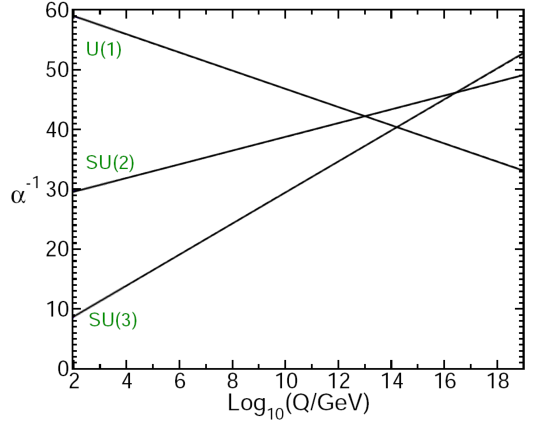
Figure 3.2: Two-loop renormalization group evolution of the inverse of the gauge couplings $\alpha_{i}(i=1,2,3)$ in the SM, as shown in [77].

We see three lines that almost cross in a small region of the plot, and again suggest that could be something new beyond the SM that make them exactly cross, therefore giving rise to the unification of interactions. And again the beauty is recovered as we introduce supersymmetry, obtaining the result of Fig. 3.3, where we see how now the three lines bend around $m_{SUSY}\sim{\cal O}\textrm{(}1\textrm{ TeV)}$ and then cross at some high scale $m_{GUT}\sim{\cal O}\textrm{(}10^{16}\textrm{ TeV)}$, and therefore the unification of the three forces related to the gauge groups of the SM is produced.

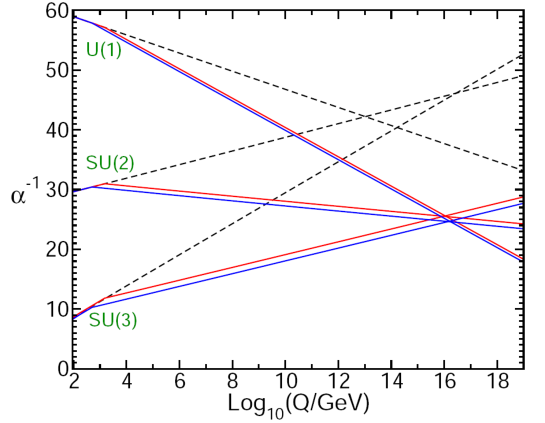
Figure 3.3: Two-loop renormalization group evolution of the inverse of the gauge couplings $\alpha_{i}(i=1,2,3)$ in the MSSM (solid lines) and in the SM (dashed lines), as shown in [77]. For the MSSM the sparticles masses are varied between 500 GeV and 1.5 TeV and $\alpha_{3}(M_{Z})$ is varied between 0.117 and 0.121.

Another appealing aspect of supersymmetry is that it is a needed ingredient for String theory, being this one of the few theories that seem good candidates to solve the unification between the quantum and the relativistic world including gravity. The introduction of supersymmetry in String theory led to a series of discoveries [78] in the eighties called the First Superstring Revolution, that draw a lot of attention to this theory pointing it as a possible correct approach to a final unification of all the interactions in physics under a unique framework.

Another interesting feature of supersymmetry is related to the dark matter problem and its connection to the conserved quantum numbers. In the SM, the baryon ($B$) and lepton ($L$) numbers are accidental conserved quantities, due to the fact that is not possible to introduce renormalizable terms in the Lagrangian able to break them. To do it we should introduce non-renormalizable 5 and 6 dimension operators as $LLHH/\Lambda_{L}$ or $QQQL/\Lambda_{B}^{2}$, as shown in [79]. Operators like these could be introduced however in a non-perturbative way by effects like instantons [80], but there would be highly suppressed. These are good news for us, since not conserving these numbers would have consequences as the proton decay (see [81] for a review). Luckily the proton is known to have a half-life larger than $2.1\times 10^{29}$ years [82]. Other measurements set also important constraints to the violation of any of these numbers (see [83, 84, 85]). However in supersymmetry is possible to introduce terms in the Lagrangian that would violate the conservation of these numbers. These terms, that will be introduced later in Eqs. 3.9 and 3.10, imply proton decay for example through the following diagram:

Figure 3.4: Proton decay to a pion and a positron, mediated by a squark. Diagram produced through terms in the supersymmetric Lagrangian violating lepton and baryon number.

leading to a partial decay width of:

$$\Gamma_{p\rightarrow e^{+}\pi^{0}}\>\sim\>m_{{\rm proton}}^{5}\sum_{i=2,3}|\lambda^{\prime 11i}\lambda^{\prime\prime 11i}|^{2}/m_{\widetilde{d}_{i}}^{4},$$ (3.6)

that means a decay of seconds for couplings $\lambda$ of order 1 and squarks masses around the TeV. The solution to this unobserved behaviour of the proton could be to ask for a new symmetry as the R-parity [86]. This is defined as the conservation of the following number:

$$P_{R}=(-1)^{3({\rm B}-{\rm L})+2s}$$ (3.7)

where $s$ is the spin of each particle.

With this new symmetry, all particles would have a defined R-parity ($+1$ for the known particles and the particles of the two Higgs doublet, and $-1$ for the supersymmetric partners), and each term of the Lagrangian should have a positive R-parity, and hence no process will change its value between the initial and final state. The consequence of this would be the absence of the worrying terms in the Lagrangian. Moreover, any interaction between particles and sparticles would always involve an even number of sparticles. This means that any decay of any sparticle would have at least one sparticle on the final state, and therefore the lightest supersymmetric particle (LSP) would be stable, being unable of decaying in other particles/sparticles. If this sparticle is neutral it could be the responsible for the unknown dark matter of the Universe, one of the main problems of the cosmology. The existence of charged LSP has very strict bounds, since the ones produced in the Big Bang would have produced bound states with some nuclei, leading to exotic isotopes whose abundance is very constrained (see e.g. [87]). The favourite candidate to dark matter within the MSSM is the lightest neutralino [45, 46] which as we will see next is a mixture between the SUSY partner of the photon and the SUSY partner of the Higgs bosons. The fact that SUSY provides good candidates for dark matter is a very convincing argument in favour of SUSY.

3.2 The Minimal Supersymmetric Standard Model

The Minimal Supersymmetric Standard Model is the simplest model that can incorporate supersymmetry and the Standard Model. The particle content of the model is shown in tables 3.1 and 3.2, where we see how it doubles the content of the SM (and also modifies the Higgs sector as explained below). In addition to the known SM particles it contains their supersymmetric partners, denoted with a tilde. The SUSY partners of the fermions are the sfermions (that are scalar bosons), and the partners of the gauge bosons are the gauginos (that are fermions). Specifically, the partners of the quarks $q$ and leptons $l$ are the squarks $\widetilde{q}$ and sleptons $\widetilde{l}$ respectively, that are spin 0 particles. The sub-indices $L$ and $R$ in the sparticles refer to the chiralities of the corresponding fermionic particles. The squarks and sleptons are scalars, and thus have no chirality. The SUSY partners of the SM gauge bosons are the gluinos $\widetilde{g}$, winos $\widetilde{W}$ and binos $\widetilde{B}$, all of them spin 1/2 particles. The last two combine after electroweak symmetry breaking to form the photinos. The Higgs sector is a bit more complex than the one of the SM. It is composed of two $SU(2)_{L}$ Higgs doublets $H_{1,2}$ instead of one, and their SUSY partners, the Higgsinos $\widetilde{H}_{1,2}$, have spin 1/2. We will explain them in detail in its corresponding section.

The gauge symmetries and a superpotential function should be defined to set the interactions of the model. The gauge groups are the ones of the SM, $SU(3)_{C}\times SU(2)_{L}\times U(1)_{Y}$, and the superpotential is:

$$W_{\rm MSSM}=\hat{U}Y^{u}\hat{Q}\hat{H}_{2}-\hat{D}Y^{d}\hat{Q}\hat{H}_{1}-\hat{E}Y^{e}\hat{L}\hat{H}_{1}+\mu\hat{H}_{1}\hat{H}_{2}\>.$$ (3.8)

where the fields are the scalars of each specific superfield appearing in table 3.1 (usually this superfield notation is used when specifying the superpotential). The flavour and gauge indices are not shown, a proper expansion of them would mean terms like $\hat{U}^{ia}\,{(Y^{u})_{i}}^{j}\,\hat{Q}_{j\alpha a}\,(\hat{H}_{2})_{\beta}\epsilon^{\alpha\beta}$ and $\mu(\hat{H}_{1})_{\alpha}(\hat{H}_{2})_{\beta}\epsilon^{\alpha\beta}$. The Yukawa couplings $Y^{u,d,e}$ are $3\times 3$ matrices in flavour space.

Other terms, changing in one unit the lepton and baryon number respectively, could be added to the superpotential compatible with the gauge groups and renormalizability as the following:

$$W_{\Delta{\rm L}=1} = {1\over 2}\lambda^{ijk}\hat{L}_{i}\hat{L}_{j}\hat{E}_{k}+\lambda^{\prime ijk}\hat{L}_{i}\hat{Q}_{j}\hat{D}_{k}+\mu^{\prime i}\hat{L}_{i}\hat{H}_{2},$$ (3.9)

$$W_{\Delta{\rm B}=1} = {1\over 2}\lambda^{\prime\prime ijk}\hat{U}_{i}\hat{D}_{j}\hat{D}_{k},$$ (3.10)

where the $\lambda$ terms could be matrices in flavour space, but they would violate lepton or baryon number respectively, triggering processes as the proton decay we commented at the end of Section 3. We will work here with a conserving R-parity MSSM so these terms will be absent (for R-parity violating SUSY see for instance [85] and [88], for bounds on these terms see also [89, 90, 47, 48]).

In the superpotential 3.8 we can recognise the Yukawa terms and a bilinear Higgs boson term, with a slight difference respect to the SM ones since here it is needed two different Higgs fields to give masses to the up and down-type particles. Therefore, the original SM spectrum will be a bit more than doubled. This requirement of having two fields comes from the fact that the superpotential must be holomorphic in the scalar fields (i.e. it should be a complex analytic function on them), and not in the complex conjugated fields. Thus, there are no terms like $\hat{U}Y^{u}\hat{Q}\hat{H}_{1}^{*}$ as we would naively had expected looking at the SM. Instead, $\hat{U}Y^{u}\hat{Q}\hat{H}_{2}$, is the one allowed here. This second Higgs doublet is also needed to cancel the triangle $SU(2)_{L}$ and $U(1)_{Y}$ anomalies produced by the fermionic partners of the Higgs bosons, i.e.

$$Tr(Y^{3})=Tr(T_{3}^{2}Y)=0,$$ (3.11)

that would not be cancelled with only one Higgs doublet, and therefore one fermionic superpartner to this Higgs doublet with $Y=1/2$ or $Y=-1/2$ spoiling this last relation (tables 3.1 and 3.2 can be used to check this cancellation, $T_{3}$ is the third component of weak isospin and $Y$ is the weak hypercharge).

The last ingredient we need for the model is the soft SUSY breaking Lagrangian:

$${\cal L}_{\rm soft}^{\rm MSSM} = -{1\over 2}\left(M_{3}\widetilde{g}\widetilde{g}+M_{2}\widetilde{W}\widetilde{W}+M_{1}\widetilde{B}\widetilde{B}+{{\rm c.c.}}\right)$$ (3.12)

$$-\left(\tilde{\cal Q}_{i}{\bar{\cal A}}^{u}_{ij}\tilde{\cal U}^{*}_{j}{\cal H}_{2}-\tilde{\cal Q}_{i}{\bar{\cal A}}^{d}_{ij}\tilde{\cal D}^{*}_{j}{\cal H}_{1}-\tilde{\cal L}_{i}{\bar{\cal A}}^{e}_{ij}\tilde{\cal E}^{*}_{j}{\cal H}_{1}+{{\rm c.c.}}\right)$$

$$-\tilde{\cal Q}^{\dagger}_{i}m_{\tilde{Q}_{ij}}^{2}\tilde{\cal Q}_{j}-\tilde{\cal L}^{\dagger}_{i}m_{\tilde{L}_{ij}}^{2}\tilde{\cal L}_{j}-\tilde{\cal U}^{*}_{i}m_{\tilde{U}_{ij}}^{2}\,\tilde{\cal U}_{j}-\tilde{\cal D}^{*}_{i}m_{\tilde{D}_{ij}}^{2}\,\tilde{\cal D}_{j}-\tilde{\cal E}^{*}_{i}m_{\tilde{E}_{ij}}^{2}\,\tilde{\cal E}_{j}$$

$$-\,m_{H_{1}}^{2}{\cal H}_{1}^{*}{\cal H}_{1}-m_{H_{2}}^{2}{\cal H}_{2}^{*}{\cal H}_{2}-\left(b{\cal H}_{2}{\cal H}_{1}+{{\rm c.c.}}\right).$$

where we have used calligraphic capital letters for the sfermion fields in the interaction basis with generation indices,

$$\tilde{\cal U}_{1,2,3}=\tilde{u}_{R},\tilde{c}_{R},\tilde{t}_{R};\quad\tilde{\cal D}_{1,2,3}=\tilde{d}_{R},\tilde{s}_{R},\tilde{b}_{R} \quad\tilde{\cal Q}_{1,2,3}=(\tilde{u}_{L}\,\tilde{d}_{L})^{T},(\tilde{c}_{L}\,\tilde{s}_{L})^{T},(\tilde{t}_{L}\,\tilde{b}_{L})^{T}$$ ; (3.13)

$$\tilde{\cal E}_{1,2,3}=\tilde{e}_{R},\tilde{\mu}_{R},\tilde{\tau}_{R} \quad\tilde{\cal L}_{1,2,3}=(\tilde{\nu}_{eL}\,\tilde{e}_{L})^{T},(\tilde{\nu}_{\mu L}\,\tilde{\mu}_{L})^{T},(\tilde{\nu}_{\tau L}\,\tilde{\tau}_{L})^{T}$$ ; (3.14)

and all the gauge indices have been omitted. All the trilinear couplings ${\bar{\cal A}}_{ij}$ and the soft squared masses $m_{ij}^{2}$ are $3\times 3$ matrices in flavour space.

Although we do not assume here any particular origin of SUSY breaking, it is reasonable to expect that all the terms with mass dimensions ($M_{3},{\bar{\cal A}}^{u}_{ij},m_{\tilde{Q}_{ij}},...$) are of the same order as the scale of SUSY breaking, generically called here and from now on $m_{SUSY}$.

3.2.1 The particles of the MSSM

In this section we summarise the different particle sectors of the model, and the mass spectrum of the particles according to the MSSM parameters. To celebrate the recent discovery [4, 5, 91, 17, 92, 16] of the Higgs boson, we start with the Higgs sector.

3.2.1.1 The Higgs sector

The Higgs sector of the MSSM is composed of two Higgs doublets:

$${\cal H}_{1} = \left(\begin{array}[]{c}{\cal H}_{1}^{0}\\[2.15277pt] {\cal H}_{1}^{-}\end{array}\right)\;=\;\left(\begin{array}[]{c}v_{1}+\frac{1}{\sqrt{2}}(\phi_{1}^{0}-i\chi_{1}^{0})\\[2.15277pt] -\phi_{1}^{-}\end{array}\right)~{},$$ (3.19)

$${\cal H}_{2} = \left(\begin{array}[]{c}{\cal H}_{2}^{+}\\[2.15277pt] {\cal H}_{2}^{0}\end{array}\right)\;=\;\left(\begin{array}[]{c}\phi_{2}^{+}\\[2.15277pt] v_{2}+\frac{1}{\sqrt{2}}(\phi_{2}^{0}+i\chi_{2}^{0})\end{array}\right)~{}.$$ (3.24)

where $v_{1}$ and $v_{2}$ are the vacuum expectation values (VEV) for the fields and the ratio between the two is defined as $\tan\beta=v_{2}/v_{1}$.

These 8 degrees of freedom, once the mass matrices are diagonalized, will produce a spectrum with the following particles:

$$h,H : \mbox{2 neutral bosons ($h$ will be the notation for the lightest one) with ${\cal CP}$}=+1$$

$$A : {\cal CP}$$ 1 neutral boson with = -1 (pseudoscalar)

$$H^{+},H^{-} :$$ 2 charged bosons

$$G,G^{+},G^{-} : \mbox{3 unphysical Goldstone bosons (which will give mass to $Z$ and $W^{\pm}$)}.$$ (3.25)

The Higgs bosons in the MSSM are needed as in the SM to break the electroweak symmetry $SU(2)_{L}\times U(1)_{Y}$ to $U(1)_{em}$ and give masses to the $Z$ and $W^{\pm}$, to break the chiral symmetry ($\psi_{L,R}\rightarrow e^{i\theta_{L,R}}\psi_{L,R}$) and give masses to the fermions (otherwise impossible since by gauge invariance is impossible to introduce mass terms for them in the Lagrangian), and are also responsible of solving the unitarity problem of the $WW$ scattering. This last problem appears when we calculate the scattering between longitudinal modes of the $W$. For instance in the SM there are contributions to this scattering from the following diagrams in Fig. 3.5, whose amplitude grows with the energy as:

Figure 3.5: $WW$ scattering without Higgs boson

$$M_{V} = -g^{2}\frac{E^{2}}{M_{W}^{2}}+\ldots,$$ (3.26)

where $g=e/\sin\theta_{W}$ and $E$ is the energy of the process. This amplitude violates unitarity at high energies. When the Higgs diagrams in Fig. 3.6 are added,

Figure 3.6: $WW$ scattering mediated by a Higgs boson

then one gets:

$$M_{TOT} = M_{V}+M_{S}=\frac{E^{2}}{M_{W}^{4}}(g_{WWH}^{2}-g^{2}M_{W}^{2})+\ldots,$$ (3.27)

When the relation between the couplings is the right one, as it happens for the SM Higgs boson $g_{WWH}=gM_{W}$, then the previously commented dangerous growing of the amplitude with energy cancels exactly and unitarity is preserved. Similar arguments apply for the MSSM Higgs sector.

To build up the MSSM Higgs sector, one starts with the Higgs potential [93] given by:

$$V\! = \!(|\mu|^{2}+m^{2}_{H_{2}})(|{\cal H}_{2}^{0}|^{2}+|{\cal H}_{2}^{+}|^{2})+(|\mu|^{2}+m^{2}_{H_{1}})(|{\cal H}_{1}^{0}|^{2}+|{\cal H}_{1}^{-}|^{2})$$ (3.28)

$$+\,[b\,({\cal H}_{2}^{+}{\cal H}_{1}^{-}-{\cal H}_{2}^{0}{\cal H}_{1}^{0})+{{\rm c.c.}}]$$

$$+{1\over 8}(g^{2}+g^{\prime 2})(|{\cal H}_{2}^{0}|^{2}+|{\cal H}_{2}^{+}|^{2}-|{\cal H}_{1}^{0}|^{2}-|{\cal H}_{1}^{-}|^{2})^{2}+{1\over 2}g^{2}|{\cal H}_{2}^{+}{\cal H}_{1}^{0*}+{\cal H}_{2}^{0}{\cal H}_{1}^{-*}|^{2}.\phantom{xxx}$$

The $\mu$ terms come from the F-term, the terms with $g$ and $g^{\prime}$ from the D-term, and the rest from the soft SUSY breaking terms.

In this potential we have 5 independent combinations of parameters (besides the known $g$ and $g^{\prime}$): $(|\mu|^{2}+m^{2}_{H_{1}})$, $(|\mu|^{2}+m^{2}_{H_{2}})$, $b$, $v_{2}\equiv\langle{\cal H}_{2}^{0}\rangle$ and $v_{1}\equiv\langle{\cal H}_{1}^{0}\rangle$. But they can be reduced to two with the following relations, which are obtained from the minimization of the potential and the value of the gauge boson masses. The minimum of the potential satisfies $\partial V/\partial{\cal H}_{1}^{0}=\partial V/\partial{\cal H}_{2}^{0}=0$. When applied to the previous potential translates into:

$$m_{H_{2}}^{2}+|\mu|^{2}-b\cot\beta-(M_{Z}^{2}/2)\cos(2\beta)\>=\>0,$$ (3.29)

$$m_{H_{1}}^{2}+|\mu|^{2}-b\tan\beta+(M_{Z}^{2}/2)\cos(2\beta)\>=\>0,$$ (3.30)

giving us two of the commented relations. On the other hand, the gauge boson masses are:

$$M_{W}^{2}=\frac{1}{2}g^{2}(v_{1}^{2}+v_{2}^{2})\qquad;\qquad M_{Z}^{2}=\frac{1}{2}(g^{\prime 2}+g^{2})(v_{1}^{2}+v_{2}^{2})\qquad;\qquad M_{\gamma}=0.$$ (3.31)

where $g=e/\sin\theta_{W}$ and $g^{\prime}=e/\cos\theta_{W}$.

As the masses are known, they fix the combination $(v_{1}^{2}+v_{2}^{2})$ and therefore we have the third relation needed to reduce the unknown parameters of our potential to two, that usually are taken as:

$$\tan\beta=v_{2}/v_{1}\quad;\quad M_{A}^{2}=-{1\over 8}(g^{2}+g^{\prime 2})(\tan\beta+\cot\beta),$$ (3.32)

where $M_{A}$ is the mass of the ${\cal CP}$-odd Higgs boson $A$. The rest of the Higgs masses are fixed in terms of these parameters at tree level.

If the equations 3.29 and 3.30 are used to work out the value of $M_{Z}$ we obtain:

$$M_{Z}^{2} = \frac{|m^{2}_{H_{1}}-m^{2}_{H_{2}}|}{\sqrt{1-\sin^{2}(2\beta)}}-m^{2}_{H_{2}}-m^{2}_{H_{1}}-2|\mu|^{2}.$$ (3.33)

If we look at the size of the parameters in this last equation we see that a problem appears. The parameters $m_{H_{1}}$ and $m_{H_{2}}$ have to do with the soft SUSY breaking scale, while $\mu$ has nothing to do with this breaking, it is a SUSY preserving parameter, and therefore one would expect it to come from a much higher scale. But if that was the situation, being of such a different orders of magnitude it would be impossible to get a cancellation between them to obtain the small value of $M_{Z}$. A popular model that solves this issue is the Next-to-Minimal Supersymmetric Standard Model (NMSSM) (for a review, see for instance [94]) which introduces a new scalar singlet that gets a VEV generating the $\mu$ term, now of the proper size to get the above commented cancellation. But even when getting the right size, we see that the cancellation should be very precise to get the right value of $M_{Z}$ in the electroweak scale. Again the need of some fine-tuning, that was precisely one of the motivations to go when going from the SM to the MSSM, reappears in our model. Anyway, as we commented when talking about the hierarchy problem, this could be understood as not being a real problem, but a hint of possible more complex models beyond the MSSM, as the one commented before.

With respect to the potential, two important inequalities should be satisfied if we want our model to work properly: First, we want our potential to be bounded from below, so the vacuum is stable. This will be satisfied thanks to the positive quartic interactions of the potential that dominate over the others terms at large value of the fields, but for the directions where the quartic terms are zero, the following condition should be satisfied in order to have a bounded potential from the interaction between the others positive and negative terms:

$$2b<2|\mu|^{2}+m^{2}_{H_{1}}+m^{2}_{H_{2}}.$$ (3.34)

Second, we want to break the electroweak symmetry, because electromagnetism is the symmetry we see in our universe. Some linear combination of ${\cal H}^{0}_{1}$ and ${\cal H}^{0}_{2}$ will have negative squared mass for ${\cal H}^{0}_{1}={\cal H}^{0}_{2}=0$ (and thus this point will be unstable, and the breaking will take place) if this relation is true:

$$b^{2}>(|\mu|^{2}+m^{2}_{H_{1}})(|\mu|^{2}+m^{2}_{H_{2}}).$$ (3.35)

If we take a look to the Renormalization Group Equations (RGE), we can see that the large Yukawa coupling for the top drives $m^{2}_{H_{2}}$ to negative values and therefore helps to satisfy the previous equation. This is another success of SUSY, since in the SM the equivalent $\mu$ term is just a free parameter and there is no theoretical reason for $\mu^{2}$ to be negative and break the electroweak symmetry. Furthermore, if we evolve the top mass from high scale down to low energy, the RGEs tell us that at some moment the evolution will stop (what is called a fixed point) [95] giving us a top Yukawa around 1, almost independently of the high scale chosen. Hence, this requirement of having a large Yukawa is also understood in SUSY, and the success is double.

Once we get the potential, we can write the mass matrix of the bosons. Since there are terms that mix the scalar bosons, the corresponding mass matrix will not be diagonal, so we have to rotate it to find the mass basis. This is performed via the orthogonal transformations:

$$\left(\begin{array}[]{c}H\\[2.15277pt] h\end{array}\right) = \left(\begin{array}[]{cc}\cos\alpha&\sin\alpha\\[2.15277pt] -\sin\alpha&\cos\alpha\end{array}\right)\left(\begin{array}[]{c}\phi_{1}^{0}\\[2.15277pt] \phi_{2}^{0}\end{array}\right)~{},$$ (3.42)

$$\left(\begin{array}[]{c}G\\[2.15277pt] A\end{array}\right) = \left(\begin{array}[]{cc}\cos\beta&\sin\beta\\[2.15277pt] -\sin\beta&\cos\beta\end{array}\right)\left(\begin{array}[]{c}\chi_{1}^{0}\\[2.15277pt] \chi_{2}^{0}\end{array}\right)~{},$$ (3.49)

$$\left(\begin{array}[]{c}G^{\pm}\\[2.15277pt] H^{\pm}\end{array}\right) = \left(\begin{array}[]{cc}\cos\beta&\sin\beta\\[2.15277pt] -\sin\beta&\cos\beta\end{array}\right)\left(\begin{array}[]{c}\phi_{1}^{\pm}\\[2.15277pt] \phi_{2}^{\pm}\end{array}\right)~{}.$$ (3.56)

The mixing angle $\alpha$ is determined through

$$\alpha={\rm arctan}\left[\frac{-(M_{A}^{2}+M_{Z}^{2})\sin\beta\cos\beta}{M_{Z}^{2}\cos^{2}\beta+M_{A}^{2}\sin^{2}\beta-m^{2}_{h,{\rm tree}}}\right]~{},~{}~{}-\frac{\pi}{2}<\alpha<0~{}.$$ (3.57)

At tree level the mass matrix of the neutral ${\cal CP}$-even Higgs bosons is given in the $\phi_{1}$-$\phi_{2}$-basis in terms of $M_{Z}$, $M_{A}$, and $\tan\beta$ by

$$M_{\rm Higgs}^{2,{\rm tree}} = \left(\begin{array}[]{cc}m_{\phi_{1}}^{2}&m_{\phi_{1}\phi_{2}}^{2}\\ m_{\phi_{1}\phi_{2}}^{2}&m_{\phi_{2}}^{2}\end{array}\right)$$ (3.60)

$$= \left(\begin{array}[]{cc}M_{A}^{2}\sin^{2}\beta+M_{Z}^{2}\cos^{2}\beta&-(M_{A}^{2}+M_{Z}^{2})\sin\beta\cos\beta\\ -(M_{A}^{2}+M_{Z}^{2})\sin\beta\cos\beta&M_{A}^{2}\cos^{2}\beta+M_{Z}^{2}\sin^{2}\beta\end{array}\right),$$ (3.63)

which by diagonalization according to Eq. (3.42) yields the tree-level Higgs boson masses

$$M_{\rm Higgs}^{2,{\rm tree}}\stackrel{{\scriptstyle\alpha}}{{\longrightarrow}}\left(\begin{array}[]{cc}m_{H,{\rm tree}}^{2}&0\\ 0&m_{h,{\rm tree}}^{2}\end{array}\right)~{},$$ (3.64)

where

$$(m_{H,h}^{2})_{\rm tree}=\frac{1}{2}\left[M_{A}^{2}+M_{Z}^{2}\pm\sqrt{(M_{A}^{2}+M_{Z}^{2})^{2}-4M_{Z}^{2}M_{A}^{2}\cos^{2}2\beta}\right]~{}.$$ (3.65)

At tree level the light Higgs boson is too light, having as upper bound to its mass the value of $M_{Z}$.

The charged Higgs boson mass is given by

$$m^{2}_{H^{\pm},{\rm tree}}=M_{A}^{2}+M_{W}^{2}~{}.$$ (3.66)

Once we have all the Higgs boson masses it is interesting to give a fast look to the couplings or at least to some features of them. Nowadays these couplings are being measured for the discovered Higgs boson, and it is important to know the differences between a SM and a MSSM Higgs boson. At tree level, the MSSM couplings can be expressed in terms of the corresponding SM couplings and some extra factors. See next some of these relations:

$$g_{hVV}=g_{HVV}^{SM}\sin(\beta-\alpha)\quad;\quad g_{HVV}=g_{HVV}^{SM}\cos(\beta-\alpha)\quad;\quad g_{AVV}=0$$ (3.67)

$$g_{hAZ}=\frac{g^{\prime}}{2c_{W}}\cos(\beta-\alpha)\quad \quad g_{HAZ}=\frac{g^{\prime}}{2c_{W}}\sin(\beta-\alpha)$$ ; (3.68)

$$g_{hb\overline{b},h\tau^{+}\tau^{-}}=g_{Hb\overline{b},H\tau^{+}\tau^{-}}^{SM}(-\frac{\sin\alpha}{\cos\beta})\quad \quad g_{ht\overline{t}}=g_{Ht\overline{t}}^{SM}\frac{\cos\alpha}{\sin\beta}$$ ; (3.69)

$$g_{Hb\overline{b},H\tau^{+}\tau^{-}}=g_{Hb\overline{b},H\tau^{+}\tau^{-}}^{SM}\frac{\cos\alpha}{\cos\beta}\quad \quad g_{Ht\overline{t}}=g_{Ht\overline{t}}^{SM}\frac{\sin\alpha}{\sin\beta}$$ ; (3.70)

$$g_{Ab\overline{b},A\tau^{+}\tau^{-}}=g_{Hb\overline{b},H\tau^{+}\tau^{-}}^{SM}\gamma_{5}\tan\beta\quad \quad g_{At\overline{t}}=g_{Ht\overline{t}}^{SM}\gamma_{5}\cot\beta$$ ; (3.71)

where $V=Z,W^{\pm}$, and the results are the same for the other two generations of fermions.

We can see how depending on the $\alpha$ and $\beta$ angles, we can obtain very different situations to the SM. For example, the coupling of the light Higgs boson with the pseudoscalar $A$ and the gauge boson $Z$ that can give rise to new phenomenology, or the huge increase we can find in the coupling with the bottom-type fermions for the large $\tan\beta$ case, that could play a very important role in the MSSM phenomenology (see e.g. [96, 97, 98, 99, 100]). Another interesting situation is the limit:

$$-\frac{\sin\alpha}{\cos\beta}\to 1\qquad;\qquad\beta-\alpha\to\pi/2$$ (3.72)

where the light Higgs boson will behave as the SM Higgs boson, being almost impossible to distinguish between the two. This situation is realised in the so called decoupling limit, for $M_{A}\gg 150$ GeV, when $h$ behaves SM-like and $M_{A}\simeq M_{H}\simeq M_{H}^{\pm}$, with the heavy Higgs bosons decoupling from the low energy electroweak physics. As an example of this limit, see the dependence of two of the tree level couplings of the light MSSM Higgs boson to the $b$ and $t$ quarks with respect to $M_{A}$ in Figs. 3.7 and 3.8. The values represented $C_{ffh}$ are the ratios between the MSSM value of the coupling divided to the corresponding SM Higgs coupling. That is, their values are 1 when the MSSM coupling coincides with the SM coupling.

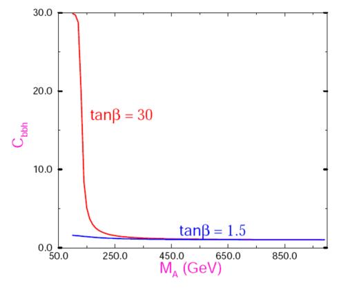
Figure 3.7: Ratio between the tree-level couplings of the MSSM and the SM between a down type fermion and the Higgs boson (light Higgs boson and the SM Higgs boson respectively). Plot obtained from [101].

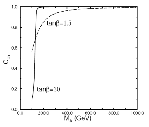
Figure 3.8: Ratio between the tree-level couplings of the MSSM and the SM between an up type fermion and the Higgs boson (light Higgs boson and the SM Higgs boson respectively). Plot obtained from [101].

Since finally we have measurements for the Higgs mass, and these will improve a lot in a close future, is important to have precision predictions for it, and for the rest of the Higgs boson parameters. In the next section we will study the one loop corrections to the Higgs boson masses, and we will see how these corrections are very important.

3.2.1.2 The Higgs sector at one-loop

In the Feynman diagrammatic (FD) approach that we are following here, the higher-order corrected ${\cal CP}$-even Higgs boson masses are derived by finding the poles of the $(h,H)$-propagator matrix. The inverse of this matrix is given by

$$\left(\Delta_{\rm Higgs}\right)^{-1}=-i\left(\begin{array}[]{cc}p^{2}-m_{H,{\rm tree}}^{2}+\hat{\Sigma}_{HH}(p^{2})&\hat{\Sigma}_{hH}(p^{2})\\ \hat{\Sigma}_{hH}(p^{2})&p^{2}-m_{h,{\rm tree}}^{2}+\hat{\Sigma}_{hh}(p^{2})\end{array}\right)~{}.$$ (3.73)

Determining the poles of the matrix $\Delta_{\rm Higgs}$ in Eq. (3.73) is equivalent to solving the equation

$$\left[p^{2}-m_{h,{\rm tree}}^{2}+\hat{\Sigma}_{hh}(p^{2})\right]\left[p^{2}-m_{H,{\rm tree}}^{2}+\hat{\Sigma}_{HH}(p^{2})\right]-\left[\hat{\Sigma}_{hH}(p^{2})\right]^{2}=0\,.$$ (3.74)

Similarly, in the case of the charged Higgs sector, the corrected Higgs mass is derived by the position of the pole in the charged Higgs propagator, which is defined by:

$$p^{2}-m^{2}_{H^{\pm},{\rm tree}}+\hat{\Sigma}_{H^{-}H^{+}}\left(p^{2}\right)=0.$$ (3.75)

To solve the previous equations, the renormalized Higgs boson self-energies are needed. Here we follow the procedure used in Refs. [102, 103] (and references therein) and review it for completeness. The parameters appearing in the Higgs potential, see Eq. (3.28), are renormalized as follows:

$$M_{Z}^{2} \to M_{Z}^{2}+\delta M_{Z}^{2}, T_{h} \to T_{h}+\delta T_{h},$$ (3.76)

$$M_{W}^{2} \to M_{W}^{2}+\delta M_{W}^{2}, T_{H} \to T_{H}+\delta T_{H},$$

$$M_{\rm Higgs}^{2} \to M_{\rm Higgs}^{2}+\delta M_{\rm Higgs}^{2}, \tan\beta\, \to\tan\beta\,(1+\delta\!\tan\!\beta\,).$$

$M_{\rm Higgs}^{2}$ denotes the tree-level Higgs boson mass matrix given in Eq. (3.63). $T_{h}$ and $T_{H}$ [are the tree-level tadpoles (i.e. the terms linear in $h$ and $H$ in the Higgs potential).

The field renormalization matrices of both Higgs multiplets can be set up symmetrically,

$$\begin{pmatrix}h\\[5.0pt] H\end{pmatrix}\to\begin{pmatrix}1+\tfrac{1}{2}\delta Z_{hh}&\tfrac{1}{2}\delta Z_{hH}\\[5.0pt] \tfrac{1}{2}\delta Z_{hH}&1+\tfrac{1}{2}\delta Z_{HH}\end{pmatrix}\cdot\begin{pmatrix}h\\[5.0pt] H\end{pmatrix}~{}.$$ (3.77)

For the mass counter term matrices we use the definitions:

$$\delta M_{\rm Higgs}^{2}=\begin{pmatrix}\delta m_{h}^{2}&\delta m_{hH}^{2}\\[5.0pt] \delta m_{hH}^{2}&\delta m_{H}^{2}\end{pmatrix}~{}.$$ (3.78)

The renormalized self-energies, $\hat{\Sigma}(p^{2})$, can now be expressed through the unrenormalized self-energies, $\Sigma(p^{2})$, the field renormalization constants and the mass counter terms. This reads for the ${\cal CP}$-even part,

$$\hat{\Sigma}_{hh}(p^{2}) =\Sigma_{hh}(p^{2})+\delta Z_{hh}(p^{2}-m_{h,{\rm tree}}^{2})-\delta m_{h}^{2},$$ (3.79a)

$$\hat{\Sigma}_{hH}(p^{2}) =\Sigma_{hH}(p^{2})+\delta Z_{hH}(p^{2}-\tfrac{1}{2}(m_{h,{\rm tree}}^{2}+m_{H,{\rm tree}}^{2}))-\delta m_{hH}^{2},$$ (3.79b)

$$\hat{\Sigma}_{HH}(p^{2}) =\Sigma_{HH}(p^{2})+\delta Z_{HH}(p^{2}-m_{H,{\rm tree}}^{2})-\delta m_{H}^{2}~{}.$$ (3.79c)

Inserting the renormalization transformation into the Higgs mass terms leads to expressions for their counter terms which consequently depend on the other counter terms introduced in (3.76).

For the ${\cal CP}$-even part of the Higgs sectors, these counter terms are:

$$\delta m_{h}^{2} =\delta M_{A}^{2}\cos^{2}(\alpha-\beta)+\delta M_{Z}^{2}\sin^{2}(\alpha+\beta)$$ (3.80a)

$$\quad+\tfrac{e}{2M_{Z}s_{\mathrm{w}}c_{\mathrm{w}}}(\delta T_{H}\cos(\alpha-\beta)\sin^{2}(\alpha-\beta)+\delta T_{h}\sin(\alpha-\beta)(1+\cos^{2}(\alpha-\beta)))$$

$$\quad+\delta\!\tan\!\beta\,\sin\beta\,\cos\beta\,(M_{A}^{2}\sin 2(\alpha-\beta)+M_{Z}^{2}\sin 2(\alpha+\beta)),$$

$$\delta m_{hH}^{2} =\tfrac{1}{2}(\delta M_{A}^{2}\sin 2(\alpha-\beta)-\delta M_{Z}^{2}\sin 2(\alpha+\beta))$$ (3.80b)

$$\quad+\tfrac{e}{2M_{Z}s_{\mathrm{w}}c_{\mathrm{w}}}(\delta T_{H}\sin^{3}(\alpha-\beta)-\delta T_{h}\cos^{3}(\alpha-\beta))$$

$$\quad-\delta\!\tan\!\beta\,\sin\beta\,\cos\beta\,(M_{A}^{2}\cos 2(\alpha-\beta)+M_{Z}^{2}\cos 2(\alpha+\beta)),$$

$$\delta m_{H}^{2} =\delta M_{A}^{2}\sin^{2}(\alpha-\beta)+\delta M_{Z}^{2}\cos^{2}(\alpha+\beta)$$ (3.80c)

$$\quad-\tfrac{e}{2M_{Z}s_{\mathrm{w}}c_{\mathrm{w}}}(\delta T_{H}\cos(\alpha-\beta)(1+\sin^{2}(\alpha-\beta))+\delta T_{h}\sin(\alpha-\beta)\cos^{2}(\alpha-\beta))$$

$$\quad-\delta\!\tan\!\beta\,\sin\beta\,\cos\beta\,(M_{A}^{2}\sin 2(\alpha-\beta)+M_{Z}^{2}\sin 2(\alpha+\beta))~{}.$$

For the field renormalization we chose to give each Higgs doublet one renormalization constant,

$${\cal H}_{1}\to(1+\tfrac{1}{2}\delta Z_{{\cal H}_{1}}){\cal H}_{1},\quad{\cal H}_{2}\to(1+\tfrac{1}{2}\delta Z_{{\cal H}_{2}}){\cal H}_{2}~{}.$$ (3.81)

This leads to the following expressions for the various field renormalization constants in Eq. (3.77):

$$\delta Z_{hh} =\sin^{2}\!\alpha\,\delta Z_{{\cal H}_{1}}+\cos^{2}\!\alpha\,\delta Z_{{\cal H}_{2}},$$ (3.82a)

$$\delta Z_{hH} =\sin\alpha\,\cos\alpha\,(\delta Z_{{\cal H}_{2}}-\delta Z_{{\cal H}_{1}}),$$ (3.82b)

$$\delta Z_{HH} =\cos^{2}\!\alpha\,\delta Z_{{\cal H}_{1}}+\sin^{2}\!\alpha\,\delta Z_{{\cal H}_{2}}~{}.$$ (3.82c)

The counter term for $\tan\beta$ can be expressed in terms of the vacuum expectation values as

$$\delta\tan\beta=\frac{1}{2}\left(\delta Z_{{\cal H}_{2}}-\delta Z_{{\cal H}_{1}}\right)+\frac{\delta v_{2}}{v_{2}}-\frac{\delta v_{1}}{v_{1}}~{},$$ (3.83)

where the $\delta v_{i}$ are the renormalization constants of the $v_{i}$:

$$v_{1}\to\left(1+\delta Z_{{\cal H}_{1}}\right)\left(v_{1}+\delta v_{1}\right),\quad v_{2}\to\left(1+\delta Z_{{\cal H}_{2}}\right)\left(v_{2}+\delta v_{2}\right)~{}.$$ (3.84)

Similarly for the charged Higgs sector, the renormalized self-energy is expressed in terms of the unrenormalized one and the corresponding counter-terms as:

$$\hat{\Sigma}_{H^{-}H^{+}}\left(p^{2}\right)=\Sigma_{H^{-}H^{+}}\left(p^{2}\right)+\delta Z_{H^{-}H^{+}}\left(p^{2}-m^{2}_{H^{\pm},{\rm tree}}\right)-\delta m_{H^{\pm}}^{2},$$ (3.85)

where,

$$\delta m_{H^{\pm}}^{2}=\delta M_{A}^{2}+\delta M_{W}^{2}$$ (3.86)

and,

$$\delta Z_{H^{-}H^{+}}=\sin^{2}\beta\,\,\delta Z_{{\cal H}_{1}}+\cos^{2}\beta\,\,\delta Z_{{\cal H}_{2}}.$$ (3.87)

The renormalization conditions are fixed by an appropriate renormalization scheme. For the mass counter terms on-shell conditions are used, resulting in:

$$\delta M_{Z}^{2}=\mathop{\mathrm{Re}}\Sigma_{ZZ}(M_{Z}^{2}),\quad\delta M_{W}^{2}=\mathop{\mathrm{Re}}\Sigma_{WW}(M_{W}^{2}),\quad\delta M_{A}^{2}=\mathop{\mathrm{Re}}\Sigma_{AA}(M_{A}^{2}).$$ (3.88)

For the gauge bosons in Eq. 3.88 $\Sigma$ denotes the transverse part of the corresponding self-energy. Since the renormalized tadpole configurations are chosen to vanish in all orders, their counter terms follow from $T_{\{h,H\}}+\delta T_{\{h,H\}}=0$:

$$\delta T_{h}=-{T_{h}},\quad\delta T_{H}=-{T_{H}}~{}.$$ (3.89)

For the remaining renormalization constants, i.e. $\delta\tan\beta$, $\delta Z_{{\cal H}_{1}}$ and $\delta Z_{{\cal H}_{2}}$, the most convenient choice is a $\overline{\rm DR}$ renormalization where:

$$\delta Z_{{\cal H}_{1}} =\delta Z_{{\cal H}_{1}}^{\overline{\rm{DR}}}\;=\;-\left[\mathop{\mathrm{Re}}\Sigma^{\prime}_{HH\;|\alpha=0}\right]^{\rm div},$$ (3.90a)

$$\delta Z_{{\cal H}_{2}} =\delta Z_{{\cal H}_{2}}^{\overline{\rm{DR}}}\;=\;-\left[\mathop{\mathrm{Re}}\Sigma^{\prime}_{hh\;|\alpha=0}\right]^{\rm div},$$ (3.90b)

$$\delta\!\tan\!\beta\, =-\frac{1}{2}(\delta Z_{{\cal H}_{2}}-\delta Z_{{\cal H}_{1}})=\delta\!\tan\!\beta\,^{\overline{\rm{DR}}}~{}.$$ (3.90c)

The corresponding renormalization scale, $\mu_{\overline{\mathrm{DR}}}$, is set to $\mu_{\overline{\mathrm{DR}}}=m_{t}$ in all numerical evaluations.

With the previous equations we can calculate the corrections to the Higgs bosons masses. If we vary all the relevant MSSM parameters we can get a corrected light Higgs mass up to 135GeV, what is perfectly compatible with the observed Higgs mass around 125GeV.

The above procedure will be used in Chapter 7 to calculate the corrections to the Higgs bosons masses coming from the supersymmetric particles with sfermion mixing.

For phenomenological purposes, it is convenient to estimate in advance the approximate value for $M_{h}$ without going through the whole renormalization procedure. In [104] a formula can be found for the leading $m_{t}^{4}$ corrections up to two-loops which works reasonably well ${\cal O}$ (5GeV) for moderate and low $\tan\beta$:

$$M_{h}^{2} = m_{h}^{2,{\rm tree}}+m_{h}^{2,\alpha}+m_{h}^{2,\alpha\alpha_{s}}$$ (3.91)

$$m_{h}^{2,\alpha} = \frac{3}{2}\frac{G_{F}\sqrt{2}}{\pi^{2}}M_{t}^{4}\left\{-{\rm ln}\left(\frac{M_{t}^{2}}{M_{S}^{2}}\right)+\frac{X_{t}^{2}}{M_{S}^{2}}\left(1-\frac{1}{12}\frac{X_{t}^{2}}{M_{S}^{2}}\right)\right\}$$ (3.92)

$$m_{h}^{2,\alpha\alpha_{s}} = -3\frac{G_{F}\sqrt{2}}{\pi^{2}}\frac{\alpha_{s}}{\pi}M_{t}^{4}\Bigg{\{}-{\rm ln^{2}}\left(\frac{M_{t}^{2}}{M_{S}^{2}}\right)$$ (3.94)

$$-\left(2+\frac{X_{t}^{2}}{M_{S}^{2}}\right){\rm ln}\left(\frac{M_{t}^{2}}{M_{S}^{2}}\right)-\frac{X_{t}}{M_{S}}\left(2-\frac{1}{4}\frac{X_{t}^{3}}{M_{S}^{3}}\right)\Bigg{\}}$$

where $X_{t}=A_{t}-\mu\cot\beta$, $A_{t}=A^{u}_{33}={\cal A}^{u}_{33}/y_{t}$, where $y_{t}$ is the top Yukawa, and $M_{S}$ is the relevant average mass, often defined as the geometric mean between $m_{\tilde{U}_{L33}}$ and $m_{\tilde{U}_{R33}}$. All of the input parameters are on-shell quantities.

In Figure 3.9 we show the values of the light Higgs boson mass calculated at tree level and with Equation 3.91 with respect to $X_{t}$. It can be seen the relevance of the loop contributions.

Figure 3.9: Light Higgs boson mass calculated at tree level (orange line) and using the two loop approximation of Equation 3.91 (blue dashed curve) with respect to $X_{t}$, with the following values: $M_{t}=173.07$ GeV, $M_{S}=M_{A}=1000$ GeV, $\tan\beta=10$. One-loop contributions from other sectors lower the light Higgs boson mass by about 10 GeV

3.2.1.3 The chargino/neutralino sector

Once the Higgs sector is studied we describe the supersymmetric partners of the Higgs bosons: the Higgsinos. Since the Higgsinos have the same quantum numbers as the electroweak gauginos, and there are mixing terms in the Lagrangian between them, then they mix giving rise to the physical particles in the final mass basis. Therefore we will study them together. The electrical charge is a well-defined quantum number so the charged particles and the neutral ones will not mix between them. The neutral Higgsinos ($\widetilde{\cal H}_{1}^{0}$ and $\widetilde{\cal H}_{2}^{0}$) mix with the neutral gauginos ($\widetilde{B}$ and $\widetilde{W}^{0}$) forming the so called neutralinos (${\tilde{\chi}}^{0}_{i}$, $i=1,2,3,4$). The charged Higgsinos ($\widetilde{\cal H}_{2}^{+}$ and $\widetilde{\cal H}_{1}^{-}$) and the charged winos ($\widetilde{W}^{+}$ and $\widetilde{W}^{-}$) will originate the charginos (${\tilde{\chi}}^{\pm}_{i}$, $i=1,2$).

According to the MSSM Lagrangian, the charginos have the following mass matrix in the interaction basis $\psi^{\pm}=(\widetilde{W}^{+},\,\widetilde{\cal H}_{2}^{+},\,\widetilde{W}^{-},\,\widetilde{\cal H}_{1}^{-})$:

$${\bf M}_{{\tilde{\chi}}^{\pm}} = \begin{pmatrix}{\bf 0}&{\bf X}^{T}\cr{\bf X}&{\bf 0}\end{pmatrix},\phantom{xx}$$ (3.95)

$${\bf X} = \begin{pmatrix}M_{2}&gv_{u}\cr gv_{d}&\mu\cr\end{pmatrix}\>=\>\begin{pmatrix}M_{2}&\sqrt{2}s_{\beta}\,M_{W}\cr\sqrt{2}c_{\beta}\,M_{W}&\mu\cr\end{pmatrix}.$$ (3.96)

This matrix is diagonalized using two $2\times 2$ unitary matrices ${\bf U}$ and ${\bf V}$ that rotate the basis with these relations:

$$\begin{pmatrix}\widetilde{\chi}^{+}_{1}\cr\widetilde{\chi}^{+}_{2}\end{pmatrix}={\bf V}\begin{pmatrix}\widetilde{W}^{+}\cr\widetilde{\cal H}_{2}^{+}\end{pmatrix},\quad\qquad\>\>\>\>\>\>\begin{pmatrix}\widetilde{\chi}^{-}_{1}\cr\widetilde{\chi}^{-}_{2}\end{pmatrix}={\bf U}\begin{pmatrix}\widetilde{W}^{-}\cr\widetilde{\cal H}_{1}^{-}\end{pmatrix},\phantom{xxx}$$ (3.97)

obtaining a diagonal matrix for each sub-matrix:

$${\bf U}^{*}{\bf X}{\bf V}^{-1}=\begin{pmatrix}m_{{\tilde{\chi}}^{\pm}_{1}}&0\cr 0&m_{{\tilde{\chi}}^{\pm}_{2}}\end{pmatrix},$$ (3.98)

being these the eigenvalues for the full mass squared matrix:

$${\bf V}{\bf X}^{\dagger}{\bf X}{\bf V}^{-1}={\bf U}^{*}{\bf X}{\bf X}^{\dagger}{\bf U}^{T}=\begin{pmatrix}m^{2}_{{\tilde{\chi}}^{\pm}_{1}}&0\cr 0&m^{2}_{{\tilde{\chi}}^{\pm}_{2}}\end{pmatrix}.$$ (3.99)

The neutralinos have this mass matrix:

$${\bf M}_{{\tilde{\chi}}^{0}}\,=\,\begin{pmatrix}M_{1}&0&-g^{\prime}v_{d}/\sqrt{2}&g^{\prime}v_{u}/\sqrt{2}\cr 0&M_{2}&gv_{d}/\sqrt{2}&-gv_{u}/\sqrt{2}\cr-g^{\prime}v_{d}/\sqrt{2}&gv_{d}/\sqrt{2}&0&-\mu\cr g^{\prime}v_{u}/\sqrt{2}&-gv_{u}/\sqrt{2}&-\mu&0\cr\end{pmatrix}.$$ (3.100)

in the electroweak basis $\psi^{0}=(\widetilde{B},\widetilde{W}^{0},\widetilde{\cal H}_{1}^{0},\widetilde{\cal H}_{2}^{0})$. The diagonalization is performed through a rotation ${\widetilde{\chi}}^{0}_{i}={\bf N}_{ij}\psi^{0}_{j}$ , that fulfils

$${\bf N}^{*}{\bf M}_{{\tilde{\chi}}^{0}}{\bf N}^{-1}\,=\,{\rm diag}(m_{{\tilde{\chi}}^{0}_{1}},m_{{\tilde{\chi}}^{0}_{2}},m_{{\tilde{\chi}}^{0}_{3}},m_{{\tilde{\chi}}^{0}_{4}}).$$ (3.101)

The lightest neutralino ${\tilde{\chi}}^{0}_{1}$ turns out to be the LSP, and is one of the favourite candidates to dark matter.

3.2.1.4 The gluino sector

The gluinos $\widetilde{g}$ are the supersymmetric partners of the gluons. As we can see in Table 3.2 they have spin 1/2, and they keep the same gauge numbers as their standard partners as it happens with the other particles. They are octet fermions, and since there are no other SUSY particles in this representation, they do not mix with other particles.

If SUSY were an exact symmetry they would be massless as the gluons, but since it is broken, it can be found a term in the soft SUSY breaking Lagrangian that give mass to them, the term $M_{3}$. Since they have not been seen in any collider yet, it can be set a lower bound to its mass (see Section 3.2.2); although this value depends on the specific values of the other supersymmetric parameters, at present one can say that the gluino mass should be above $\sim{\cal O}$ (1 TeV).

3.2.1.5 The squark sector

As shown in table 3.1, the supersymmetric partners of the quarks are the squarks $({\widetilde{u}}_{L}\>\>\>{\widetilde{d}}_{L})$, ${\widetilde{u}}^{*}_{R}$, ${\widetilde{d}}^{*}_{R}$ (and the same for the other two generations). We recall again that the squarks are $0$ spin bosons. The sub-indices $L$ and $R$ of the squarks are just a reminder of the chirality of the corresponding fermionic partners. The squarks are scalars, and thus have no chirality.

In order to proceed with the squarks, let us look first to the partner quarks. Starting with our Lagrangian, expressed in the interaction basis, we know that the different families of quarks will mix with each other. Therefore the final mass states will be different from these starting ones. To diagonalize the mass matrix, the basis should be rotated from the $SU(2)$ (interaction) eigenstate basis, $q^{\rm int}_{L,R}$, to the (physical) mass eigenstate basis, $q_{L,R}^{\rm phys}$, by unitary transformations, $V^{u,d}_{L,R}$:

$$\left(\begin{array}[]{c}u^{\rm phys}_{L,R}\\ c^{\rm phys}_{L,R}\\ t^{\rm phys}_{L,R}\end{array}\right)=V^{u}_{L,R}\left(\begin{array}[]{c}u^{\rm int}_{L,R}\\ c^{\rm int}_{L,R}\\ t^{\rm int}_{L,R}\end{array}\right)~{},~{}~{}~{}~{}\left(\begin{array}[]{c}d^{\rm phys}_{L,R}\\ s^{\rm phys}_{L,R}\\ b^{\rm phys}_{L,R}\end{array}\right)=V^{d}_{L,R}\left(\begin{array}[]{c}d^{\rm int}_{L,R}\\ s^{\rm int}_{L,R}\\ b^{\rm int}_{L,R}\end{array}\right)~{},$$ (3.102)

such that the quark Yukawa coupling and mass matrices in the physical basis are:

$$V^{u}_{L}Y^{u*}V^{u\dagger}_{R} = {\rm diag}(y_{u},y_{c},y_{t})={\rm diag}\left(\frac{m_{u}}{v_{2}},\frac{m_{c}}{v_{2}},\frac{m_{t}}{v_{2}}\right),$$ (3.103)

$$V^{d}_{L}Y^{d*}V^{d\dagger}_{R} = {\rm diag}(y_{d},y_{s},y_{b})={\rm diag}\left(\frac{m_{d}}{v_{1}},\frac{m_{s}}{v_{1}},\frac{m_{b}}{v_{1}}\right).$$ (3.104)

The quark flavour mixing that these rotations imply, and that is measured in the experiments, will be encoded in the Cabibbo-Kobayashi-Maskawa (CKM) matrix, defined as usual as,

$$V_{\rm CKM}=V^{u}_{L}V^{d\dagger}_{L}.$$ (3.105)

Since the quarks and squarks belong to the same superfield, the same terms that we had to diagonalize for the quarks will be present for the part of the Lagrangian of the squarks, and thus the same rotation will be needed for them. The squarks are then rotated, parallel to the quarks, from the interaction basis, ${\tilde{q}}^{\rm int}_{L,R}$ to what is called the Super-CKM (SCKM) basis, ${\tilde{q}}_{L,R}$, by

$$\left(\begin{array}[]{c}\tilde{u}_{L,R}\\ \tilde{c}_{L,R}\\ \tilde{t}_{L,R}\end{array}\right)=V^{u}_{L,R}\left(\begin{array}[]{c}\tilde{u}^{\rm int}_{L,R}\\ \tilde{c}^{\rm int}_{L,R}\\ \tilde{t}^{\rm int}_{L,R}\end{array}\right)~{},~{}~{}~{}\left(\begin{array}[]{c}\tilde{d}_{L,R}\\ \tilde{s}_{L,R}\\ \tilde{b}_{L,R}\end{array}\right)=V^{d}_{L,R}\left(\begin{array}[]{c}\tilde{d}^{\rm int}_{L,R}\\ \tilde{s}^{\rm int}_{L,R}\\ \tilde{b}^{\rm int}_{L,R}\end{array}\right)~{}.$$ (3.106)

The minimal version of our supersymmetric model with respect to the flavour, the so-called minimal flavour violation hypothesis [58], defines the $V_{\rm CKM}$ matrix as the only source of flavour violation for the squark sector, as will be explained with more detail in Section 4.3.2. This MFV case will imply that the squarks in the Super-CKM basis are already the physical mass eigenstates. However in this study we will go beyond the MFV hypothesis and explore the limits of flavour in a more general context of Non Minimal Flavour Violation. This implies that in NMFV one has to perform a second rotation to reach the squark physical basis. The general parametrization of flavour mixing for the squarks in this NMFV case which is our chosen scenario will be defined in Section 5.1 and the mass matrices for that case will also be defined there.

3.2.1.6 The slepton sector

The sleptons $({\widetilde{\nu}}\>\>{\widetilde{e}}_{L})$ and ${\widetilde{e}}^{*}_{R}$ (and the same for the other two generations), are the $0$ spin bosons supersymmetric partners of the leptons, as shown in table 3.1.

When dealing with the squarks we saw how to arrive to the mass eigenstate basis by first performing a rotation from the eigenstate basis to an intermediate basis called SCKM, parallel to the rotation needed to diagonalize the quarks. When considering the leptons, the neutrinos in the MSSM as in the SM have no mass, thus this first rotation is not needed. Therefore when dealing with our chosen NMFV scenarios that incorporate general slepton flavour mixing, the sleptons will be diagonalized by one-step rotation matrices that will take them from the interaction eigenstate basis to the final mass basis. This will be treated carefully in Section 5.1. A brief introduction about neutrino masses and mixing in the lepton sector, will be presented in Section 4.1.2.

3.2.2 Experimental searches of MSSM particles and constraints

In Figure 3.10 and the top row of 3.12 there can be seen some of the present bounds for the SUSY masses from the sparticles searches by ATLAS [47]. In the plot of Fig. 3.10 it is collected a summary of the mass reach of a selection of searches for the 7 and 8 TeV data with a exclusion at the 95% CL. In the top left plot of Fig. 3.12 is presented the 95% CL exclusion limits for 8 TeV analyses for a simplified model where a pair of gluinos decays promptly via off-shell stop to four top quarks and two lightest neutralinos (LSP), in the gluino-neutralino mass plane. In the top right plot of Fig. 3.12 is shown the exclusion limits at 95% CL from 8 TeV data from electroweak production of charginos and neutralinos and the decay via four different modes, in the chargino-neutralino mass plane (the details are in [105]).

From these graphs, and taking in account than these limits are obtained under specific assumptions for each analysis, we see how the lower bound for the mass of the gluinos is around 1 TeV or even larger, and the one for the third generation squarks is located around 500 GeV (in some specific models not shown here is possible to have lighter squarks as for example stops around 200 GeV). In the plot of top left of Fig. 3.12 we see that depending on the mass of the LSP the lower bound for the gluino mass varies from 0.9 to 1.4 TeV. In the top right of Fig. 3.12 also a dependence on the LSP mass is shown for the chargino mass lower bound, varying it from 300 to 620 GeV, considering than the lightest chargino is degenerate with the second lightest neutralino, and a electroweak production of the LSP.

In Figure 3.11 and the bottom row of Figure 3.12 there are presented the mass exclusion limits obtained by CMS in the search of sparticles [48]. The plot in Figure 3.11 shows a selection of mass exclusion limits for different sparticles in R-parity conserving scenarios for the 7 and 8 TeV data, with the conditions for the mother particle and the LSP: m(LSP) = 0 GeV (right bands) or m(mother) - m(LSP) = 200 GeV (left bands). The bottom left graph of Figure 3.12 shows the exclusion limits for the 8 TeV analyses for a simplified model where a pair of gluinos decays promptly via off-shell stop to four top quarks and two lightest neutralinos (LSP), in the gluino-neutralino mass plane. In the bottom right plot of Figure 3.12 there can be seen the exclusion limits from 8 TeV data from electroweak production of charginos and neutralinos and the decay via six different modes, in the chargino-neutralino mass plane.

The results from CMS are very similar to the ones from ATLAS. The higher limits are in ATLAS as compared with CMS a bit heavier for some specific gluino cases, and a bit lower in some electroweak productions of charginos and neutralinos.

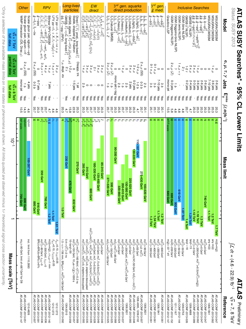
Figure 3.10: Overall summary of SUSY searches in ATLAS. Plot taken from [47]

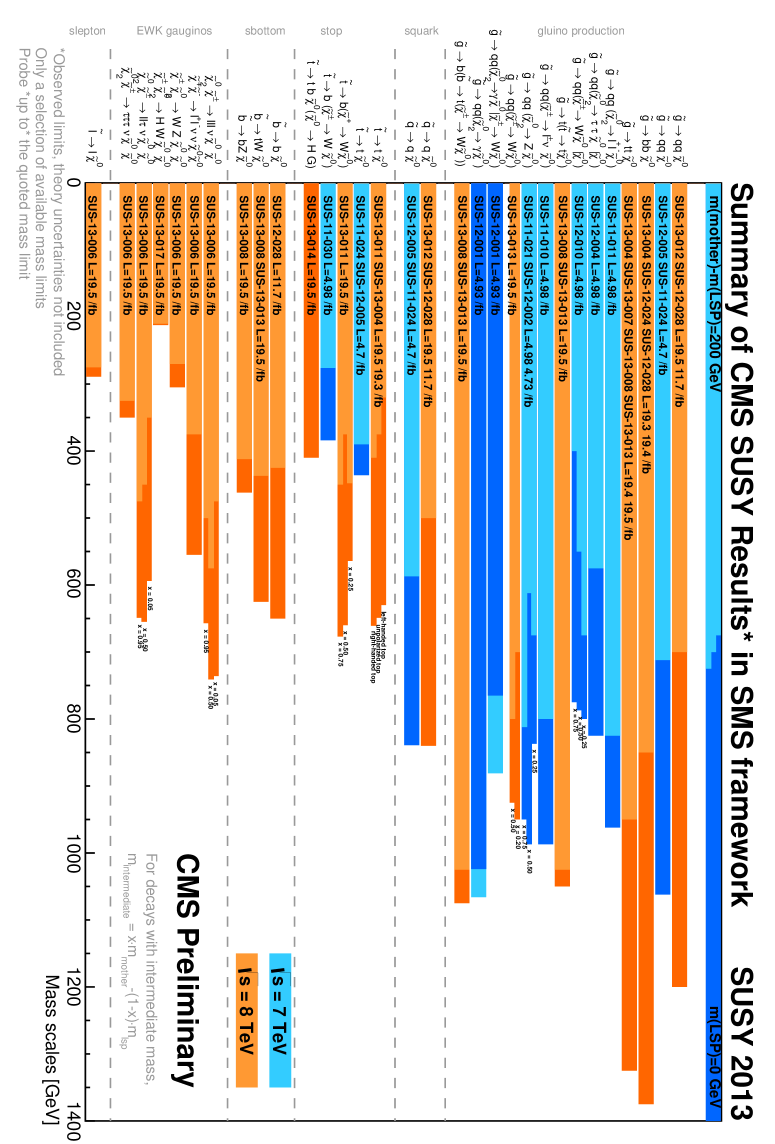
Figure 3.11: Summary of SUSY searches for R-parity conserving scenarios in CMS. Plot taken from [48]

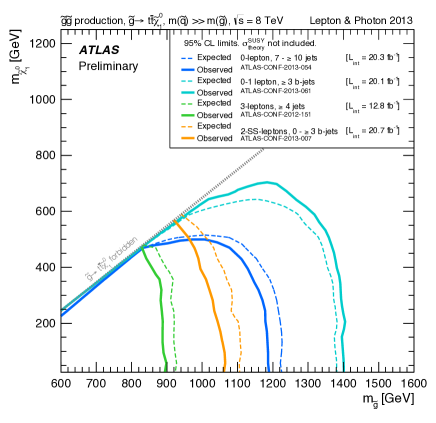
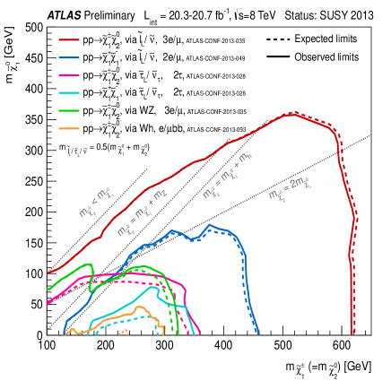
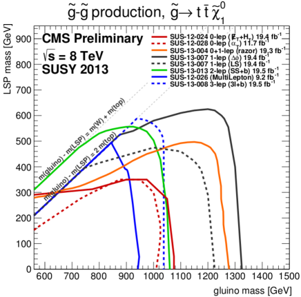
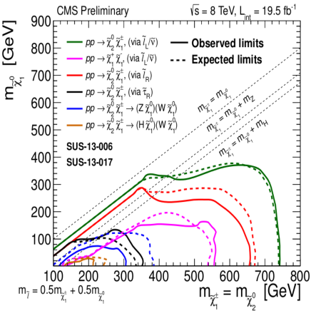
Figure 3.12: SUSY searches in ATLAS (top row) and CMS (bottom row): Exclusion limits for gluino-mediated stop production decaying to a top and a neutralino (top left). Electroweak chargino-neutralino production (top right). Exclusion limits for gluino-mediated stop production decaying to a top and a neutralino (bottom left). Electroweak chargino-neutralino production (bottom right). More details in the text. Plots taken from [47] and [48]

With respect to the Higgs bosons, since we are assuming that the discovered Higgs boson is the neutral lightest one of the MSSM, the other 4 Higgs bosons should still be found in the experiments. The charged Higgs have been searched for example through its decay to $\tau\nu$ [106, 107, 108], and through the decay to $c\bar{s}$ [109], excluding masses at the 95% CL from 90 to 160 GeV approximately. The heavy neutral Higgs bosons have been also searched, for example through the decays into a pair $\mu^{+}\mu^{-}$ or $\tau^{+}\tau^{-}$, excluding a significant part of the $M_{A}-\tan\beta$ parameter space (see results in [110, 111, 112, 113, 114]).

Chapter 4 The flavour of particles: a window to new physics

Before entering into technical details, the word flavour already captures the core of the issue. Flavour suggests a quality of the objects that make them different one from each other, a different way to feel and interact with each of them, and behind it, a capricious arbitrariness in its existence and its diversity. Let us see how particles taste.

In the spectrum of particle physics, we find copies of the elementary fermions with the same SM gauge quantum numbers but with different masses. This leads to the concept of flavour, a new feature of particles. Within the SM we find six different flavours of quarks, up, charm and top flavours having electric charge $+2/3e$ and down, strange and bottom flavours having $-1/3e$. For leptons, there are three flavours, $e$, $\mu$ and $\tau$ with $-e$ electric charge, and three flavours $\nu_{e}$, $\nu_{\mu}$ and $\nu_{\tau}$ with zero charge. This opens a set of questions as: why the number of flavours is precisely this? what is the origin of flavour? why these mass and mixing patterns of leptons and quarks? is the mass the only difference between generations? why the rates of flavour changing neutral current processes are so much suppressed in Nature? These questions and others remain unanswered but have been studied exhaustively during many years, allowing us to know the structure of flavour of the SM at present with precision and also its phenomenology. As other unknown answers, they open a path for new physics, and of course for the search of supersymmetry. In the following sections it will be shortly reviewed some flavour issues in the Standard Model and we will also comment on flavour beyond the SM.

4.1 Flavour in the Standard Model

The fermions in the SM appear as 3 families of particles, with the same gauge properties, but with different masses. The model to describe it needs at least 13 parameters if we treat the neutrinos as massless: 9 fermion masses, 3 mixing angles and 1 complex phase; and one then adds 3 masses, 3 mixing angles and 1 or 3 phases if we treat the neutrinos as massive Dirac or Majorana particles respectively.

We will start with a short review of the basic features of flavour in the quark sector, and after it we will focus on the lepton sector.

4.1.1 Flavour in the quark sector

The mixing between the different flavour generations comes from the non-diagonality of the mass matrices in the interactions basis. This is due to the Yukawa interactions between the Higgs bosons once they get a VEV and the quarks with non-diagonal Yukawa matrices. The relevant Lagrangian is:

$$\mathcal{L}_{YW}=-\bar{\cal Q}^{\rm int}_{L}Y^{u}\tilde{\Phi}{\cal U}^{\rm int}_{R}-\bar{\cal Q}^{\rm int}_{L}Y^{d}\Phi{\cal D}^{\rm int}_{R}+h.c.$$ (4.1)

where $Y^{u}$ and $Y^{d}$ are $3\times 3$ Yukawa coupling matrices, $\Phi=\left(\begin{array}[]{c}\phi^{+}\\ \phi^{0}\end{array}\right)$ is the SM Higgs doublet, $\tilde{\Phi}=i\sigma_{2}\Phi^{*}=\left(\begin{array}[]{c}\phi^{0*}\\ -\phi^{-}\end{array}\right)$ and the interaction eigenstates are:

$${\cal Q}^{\rm int}_{L}=\left(\begin{array}[]{c}{\cal U}^{\rm int}_{L}\\ {\cal D}^{\rm int}_{L}\end{array}\right)\quad;\quad{\cal U}^{\rm int}_{R}=\left(\begin{array}[]{c}u^{\rm int}_{R}\\ c^{\rm int}_{R}\\ t^{\rm int}_{R}\end{array}\right)\quad;\quad{\cal D}^{\rm int}_{R}=\left(\begin{array}[]{c}d^{\rm int}_{R}\\ s^{\rm int}_{R}\\ b^{\rm int}_{R}\end{array}\right)$$ (4.2)

where

$${\cal U}^{\rm int}_{L}=\left(\begin{array}[]{c}u^{\rm int}_{L}\\ c^{\rm int}_{L}\\ t^{\rm int}_{L}\end{array}\right)\quad;\quad{\cal D}^{\rm int}_{L}=\left(\begin{array}[]{c}d^{\rm int}_{L}\\ s^{\rm int}_{L}\\ b^{\rm int}_{L}\end{array}\right).$$ (4.3)

To obtain the mass eigenstates one rotates the quarks to the physical mass basis with the following rotations:

$$\left(\begin{array}[]{c}u^{\rm phys}_{L,R}\\ c^{\rm phys}_{L,R}\\ t^{\rm phys}_{L,R}\end{array}\right)=V^{u}_{L,R}\left(\begin{array}[]{c}u^{\rm int}_{L,R}\\ c^{\rm int}_{L,R}\\ t^{\rm int}_{L,R}\end{array}\right)~{},~{}~{}~{}~{}\left(\begin{array}[]{c}d^{\rm phys}_{L,R}\\ s^{\rm phys}_{L,R}\\ b^{\rm phys}_{L,R}\end{array}\right)=V^{d}_{L,R}\left(\begin{array}[]{c}d^{\rm int}_{L,R}\\ s^{\rm int}_{L,R}\\ b^{\rm int}_{L,R}\end{array}\right)~{},$$ (4.4)

and then one obtains the diagonal quark masses and Yukawa couplings:

$$\frac{v}{\sqrt{2}}{\rm diag}\left(m_{u},m_{c},m_{t}\right) = {\rm diag}(y_{u},y_{c},y_{t})=V^{u}_{L}Y^{u*}V^{u\dagger}_{R},$$ (4.5)

$$\frac{v}{\sqrt{2}}{\rm diag}\left(m_{d},m_{s}m_{b}\right) = {\rm diag}(y_{d},y_{s},y_{b})=V^{d}_{L}Y^{d*}V^{d\dagger}_{R}.$$ (4.6)

where $v=\langle\phi^{0}\rangle$ is the VEV of the SM Higgs boson.

With respect to the electroweak forces, the photon and the $Z$ boson mediated currents conserve flavour, but the $W^{\pm}$ ones connect the different generations. This can be seen in the Lagrangian after the change of basis as follows. The relevant Lagrangian of the interactions between the gauge bosons and the fermions in the SM is given by:

$$\mathcal{L}_{\psi} = \sum_{\psi}i\bar{\psi}\gamma^{\mu}D_{\mu}\psi=\sum_{\psi}i\bar{\psi}\gamma^{\mu}\left(\partial_{\mu}-igT\cdot W_{\mu}-ig^{\prime}YB_{\mu}\right)\psi$$ (4.16)

$$= i\bar{\psi}\gamma^{\mu}\left\{\left(\begin{array}[]{cc}\partial_{\mu}&0\\ 0&\partial_{\mu}\end{array}\right)+\left(\begin{array}[]{cc}0&\frac{-ig}{2}\left(W_{1\mu}-iW_{2\mu}\right)\\ \frac{-ig}{2}\left(W_{1\mu}+iW_{2\mu}\right)&0\end{array}\right)\right.$$

$$\left.+\left(\begin{array}[]{cc}\frac{-ig}{2}W_{3\mu}&0\\ 0&\frac{ig}{2}W_{3\mu}\end{array}\right)+\left(\begin{array}[]{cc}-ig^{\prime}YB_{\mu}&0\\ 0&-ig^{\prime}YB_{\mu}\end{array}\right)\right\}\psi$$

After breaking the electroweak symmetry the physical states are

$$W_{\mu}^{\pm}\equiv\frac{1}{\sqrt{2}}\left(W_{\mu}^{1}\mp iW_{\mu}^{{}^{2}}\right)\quad;\quad Z_{\mu}\equiv\cos\theta_{W}W_{\mu}^{{}^{3}}-\sin\theta_{W}B_{\mu}\quad;\quad A_{\mu}\equiv\sin\theta_{W}W_{\mu}^{{}^{3}}+\cos\theta_{W}B_{\mu}$$ (4.17)

where the gauge couplings are $g=\frac{e}{\sin\theta_{W}}$, $g^{\prime}=\frac{e}{\cos\theta_{W}}$. In the electroweak basis for the quark states the weak interaction Lagrangian is then:

$$\mathcal{L}^{\rm int}_{W} = \frac{g}{\sqrt{2}}\left\{W^{+}_{\mu}\bar{\cal{U}}^{\rm int}_{L}\gamma_{\mu}{\cal{D}}^{\rm int}_{L}+W^{-}_{\mu}\bar{\cal{D}}^{\rm int}_{L}\gamma_{\mu}{\cal{U}}^{\rm int}_{L}\right\}+$$ (4.18)

$$\frac{g}{c_{W}}Z_{\mu}\left\{g^{u}_{L}\bar{\cal{U}}^{\rm int}_{L}\gamma_{\mu}{\cal{U}}^{\rm int}_{L}+g^{u}_{R}\bar{\cal{U}}^{\rm int}_{R}\gamma_{\mu}{\cal{U}}^{\rm int}_{R}+g^{d}_{L}\bar{\cal{D}}^{\rm int}_{L}\gamma_{\mu}{\cal{D}}^{\rm int}_{L}+g^{d}_{R}\bar{\cal{D}}^{\rm int}_{R}\gamma_{\mu}{\cal{D}}^{\rm int}_{R}\right\}$$

where $g^{u}_{L}=(\frac{1}{2}-\frac{2}{3}s_{w}^{2})$, $g^{u}_{R}=-\frac{2}{3}s_{w}^{2}$, $g^{d}_{L}=(-\frac{1}{2}+\frac{1}{3}s_{w}^{2})$ and $g^{d}_{R}=\frac{1}{3}s_{w}^{2}$. Finally, after the rotation to the mass basis the neutral currents remain flavour diagonal, but charged currents change, giving rise to intergenerational interactions due to the non-diagonal matrix $V_{CKM}$:

$$\mathcal{L}^{\rm int}_{W} = \frac{g}{\sqrt{2}}\left\{W^{+}_{\mu}\bar{\cal{U}}^{\rm phys}_{L}\gamma_{\mu}V_{CKM}{\cal{D}}^{\rm phys}_{L}+W^{-}_{\mu}\bar{\cal{D}}^{\rm phys}_{L}\gamma_{\mu}V^{+}_{CKM}{\cal{U}}^{\rm phys}_{L}\right\}+$$ (4.19)

$$\frac{g}{c_{W}}Z_{\mu}\left\{g^{u}_{L}\bar{\cal{U}}^{\rm phys}_{L}\gamma_{\mu}{\cal{U}}^{\rm phys}_{L}+g^{u}_{R}\bar{\cal{U}}^{\rm phys}_{R}\gamma_{\mu}{\cal{U}}^{\rm phys}_{R}+\right.$$

$$\left.\phantom{\frac{g}{c_{W}}Z_{\mu}\{}g^{d}_{L}\bar{\cal{D}}^{\rm phys}_{L}\gamma_{\mu}{\cal{D}}^{\rm phys}_{L}+g^{d}_{R}\bar{\cal{D}}^{\rm phys}_{R}\gamma_{\mu}{\cal{D}}^{\rm phys}_{R}\right\},$$

where,

$$V_{\rm CKM}=V^{u}_{L}V^{d\dagger}_{L}.$$ (4.20)

This change of flavour among generations in the SM is therefore encoded in the Cabibbo-Kobayashi-Maskawa (CKM) matrix [24, 25] $V_{CKM}$.

Although this flavour changing appears in the SM at tree level only in the charged currents, at one loop level it is also present in the neutral currents. However, it is a very tiny effect due to the GIM-mechanism [115], which leads to suppression factors of flavour changing neutral currents (FCNC) given by the small ratio of the involved squared mass quark differences divided by the squared $W^{\pm}$ mass. For the third generation this ratio is not so small, but is compensated by the corresponding entries in the CKM matrix involving the mixings between the third and the other generations that are small.

4.1.1.1 The CKM matrix

The CKM matrix is a unitary $3\times 3$ matrix, and it is parametrized in a standard way as:

$$V_{\rm CKM}=\left(\begin{array}[]{ccc}V_{ud}&V_{us}&V_{ub}\\ V_{cd}&V_{cs}&V_{cb}\\ V_{td}&V_{ts}&V_{tb}\end{array}\right)=\left(\begin{array}[]{ccc}c_{12}c_{13}&s_{12}c_{13}&s_{13}e^{-i\delta}\\ -s_{12}c_{23}-c_{12}s_{23}s_{13}e^{i\delta}&c_{12}c_{23}-s_{12}s_{23}s_{13}e^{i\delta}&s_{23}c_{13}\\ s_{12}s_{23}-c_{12}c_{23}s_{13}e^{i\delta}&-s_{23}c_{12}-s_{12}c_{23}s_{13}e^{i\delta}&c_{23}c_{13}\end{array}\right)\,,$$ (4.21)

where $c_{ij}=\cos\theta_{ij}$, $s_{ij}=\sin\theta_{ij}$ ($i,j=1,2,3$), $\theta_{12}$, $\theta_{13}$ and $\theta_{23}$ are the 3 real mixing angles, and $\delta$ is the ${\cal CP}$ violation phase. $c_{ij}$ and $s_{ij}$ can all be chosen to be positive and $\delta$ may vary in the range $0\leq\delta\leq 2\pi$.

Given that $\theta_{12}$, $\theta_{13}$ and $\theta_{23}$ are known to be small from experiment, there is a hierarchy among the CKM elements, so it is common to use another parametrization that reflects this. This is the Wolfenstein version [116] defined by

$$V_{\rm CKM}=\left(\begin{array}[]{ccc}1-{\lambda^{2}\over 2}&\lambda&A\lambda^{3}(\varrho-i\eta)\\ -\lambda&1-{\lambda^{2}\over 2}&A\lambda^{2}\\ A\lambda^{3}(1-\varrho-i\eta)&-A\lambda^{2}&1\end{array}\right)+{\cal{O}}(\lambda^{4})\,,$$ (4.22)

being it an expansion on $\lambda\sim|V_{us}|\approx 0.22$. This is a more phenomenological parametrization, using in its structure information about the relative sizes of the different terms of the matrix.

These last set of parameters can be chosen in different ways, but the standard definition is the following [117]:

$$\lambda\equiv s_{12}\,,\qquad A\lambda^{2}\equiv s_{23}\,,\qquad A\lambda^{3}(\varrho-i\eta)\equiv s_{13}e^{-i\delta}$$ (4.23)

and therefore

$$\varrho=\frac{s_{13}}{s_{12}s_{23}}\cos\delta,\qquad\eta=\frac{s_{13}}{s_{12}s_{23}}\sin\delta.$$ (4.24)

The elements of the CKM matrix are obtained through different measurements, for a review and references to each measurement see for instance [118]. In Table 4.1 can be found a summary of all the elements and their related processes:

$|V_{ud}|$ is obtained from superallowed (between two members of an isospin multiplet) $0^{+}\rightarrow 0^{+}$ nuclear decays which is theoretically clean. They depend only on the vector part of the weak interaction, and therefore taking into account the Conserved Vector Current (CVC) hypothesis, the value should not depend on the specific nuclei involved and its nuclear structure values and uncertainties. This has been measured for example in the PIBETA experiment [119]. The CKM element can be also obtained from the neutron lifetime.

$|V_{us}|$ is extracted from different measurements: without relying in other CKM elements from various $K\to\pi\ell\nu$ decays (to ensure that lifetimes and form factors are not affecting the value) or from $\tau\to K\nu_{\tau}$; from the ratio $|V_{us}|/|V_{ud}|$ from the decays $K\to\mu\nu/\pi\to\mu\nu$ and $\tau\to K\nu/\tau\to\pi\nu$. Measurements can be found for example from KLOE [120] or BaBar [121].

$|V_{cd}|$ can be obtained from $D\to\pi l\nu$ (as in CLEO [122] and Belle [123])and from the most precise neutrino interactions as $\nu N\to c\mu^{+}\mu^{-}X$ (in CHORUS [124]).

$|V_{cs}|$ is measured from $D_{S}$ decays in leptons as $D_{s}\to\tau\nu$ and $D_{s}\to\mu\nu$, as the average made from the measurements of CLEO, BaBar and Belle [125]. To calculate the value of the CKM element, other quantities are needed, as for example the decay constant $f_{D_{s}}$, calculated using lattice QCD, and whose uncertainty dominates the error. Another way to obtain the element is through the semileptonic decay $D\to Kl\nu$, as measured by BaBar [126], Belle [123] and CLEO [122].

$|V_{cb}|$ can be determined from exclusive and inclusive semileptonic decays of $B$ mesons to charm, being the inclusive ones the most precise. A review of the measurements and an average can be read in [127].

$|V_{ub}|$ can be obtained as the previous element, from semileptonic $B$ decays (see the same reference [127]), but also from the $B\to\tau\nu$ decay.

$|V_{td}|$ and $|V_{ts}|$ can not be measured from the equivalent decays of the previous cases to the top case. In general these are not likely to be precisely measured in tree level decays, but can be obtained from $B-\bar{B}$ oscillations or rare decays of $B$ or $K$ mesons, with tops in the internal loops. Ratios of processes involving the two elements are measured to eliminate hadronic uncertainties present in the measurement of each CKM element by itself. From these ratios it can be extracted the ratio of the CKM elements. $B\rightarrow X_{s}\gamma$ and $B_{s}\rightarrow\mu^{+}\mu^{-}$ are sensitive to the product of $|V_{ts}|$ and another element. Other decays could be used, but with much less precision.

$|V_{tb}|$ can be measured directly from the single top quark production cross section as measured by D0 [128], CDF [129] and CMS [130]. Bounds to its value can be obtained from the top decay into W.

CKM	Process
$|V_{ud}|$	$0^{+}\to 0^{+}$ transitions
$|V_{us}|$	$K\to\pi\ell\nu$
	$\tau\to K\nu_{\tau}$
$|V_{us}|/|V_{ud}|$	$K\to\mu\nu/\pi\to\mu\nu$
	$\tau\to K\nu/\tau\to\pi\nu$
$|V_{cd}|$	$D\to\pi l\nu$
	$\nu N\to c\mu^{+}\mu^{-}X$
$|V_{cs}|$	$D_{s}\to\tau\nu$
	$D_{s}\to\mu\nu$
	$D\to Kl\nu$
$|V_{ub}|$	semileptonic $B$ decays
	$B\to\tau\nu$
$|V_{cb}|$	semileptonic $B$ decays
$|V_{td}|$ and $|V_{ts}|$	$\Delta M_{B_{d}}$
	$\Delta M_{B_{s}}$
	rare $B$ and $K$ decays
$|V_{tb}|$	top production

Table 4.1: CKM elements and main processes where their values are measured

4.1.1.2 The unitarity triangles

Although we can not predict the values of the CKM elements, we know that if there is no new physics beyond the SM the matrix should be unitary, and therefore checking its unitarity is a way to look for physics beyond the SM. The unitarity conditions are usually represented in what is called unitarity triangles. These conditions imply:

$$\sum_{\alpha=1}^{3}V_{\alpha i}V_{\alpha j}^{*}=0~{},~{}~{}i\neq j,$$ (4.25)

$$\sum_{i=1}^{3}V_{\alpha i}V_{\beta i}^{*}=0~{},~{}~{}\alpha\neq\beta.$$ (4.26)

where Greek subscripts run over the up-type quarks $u,c$ and $t$, while Latin ones run over the down-type quarks $d,s$ and $b$. From these equations it follows for example:

$$V_{ud}V_{ub}^{*}+V_{cd}V_{cb}^{*}+V_{td}V_{tb}^{*}=0.$$ (4.27)

This condition (and the others six of 4.25) can be represented in the complex plane by a triangle as the one in figure 4.1

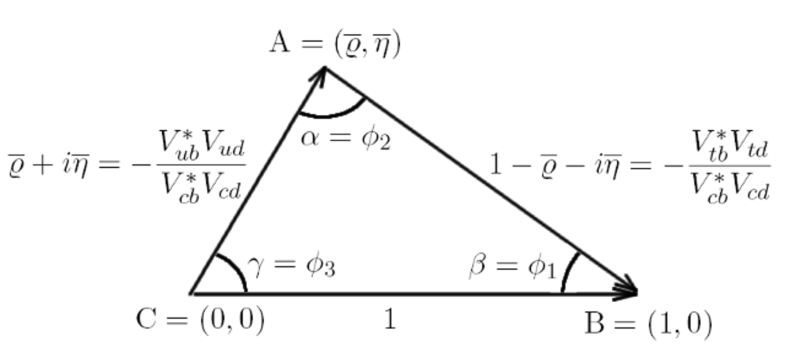
Figure 4.1: Sketch of the unitarity triangle

where

$$\overline{\varrho}+i\overline{\eta}\equiv\overrightarrow{\mathrm{CA}}=-\frac{V^{*}_{ub}V_{ud}}{V^{*}_{cb}V_{cd}},$$ (4.28)

$$\overrightarrow{\mathrm{AB}}=-\frac{V^{*}_{tb}V_{td}}{V^{*}_{cb}V_{cd}}=1-\overline{\varrho}-i\overline{\eta}\,,$$

$$\overrightarrow{\mathrm{CB}}=1\,.$$ (4.29)

and thus the sides and angles of the triangles are determined by the CKM elements, and obtained from experiments. If we find that any of these triangles do not close that would be a signal of new physics. The areas of all the six triangles are the same, and it is a measurement of ${\cal CP}$ violation

The triangles can be determined by many different experimental measurements. Combining all these data with their different sources, methods, sizes, and errors is a complex work. The two main groups that do it are the UTfit [131] and the CKMfitter [132]. The first one uses a Bayesian approach to combine the data (explained for example in [133]) while the second one uses a frequentist approach with a scheme to treat the theoretical systematics called Rfit (explained in [134]). The last results for the two collaborations are collected in Figure 4.2 ([135] Winter 2013/Pre-Moriond 2013 for UTfit; and [136] FPCP13 for CKMfitter). The results for UTfit can be found in [135]. The last results and inputs used for CKMfitter can be found in [137].

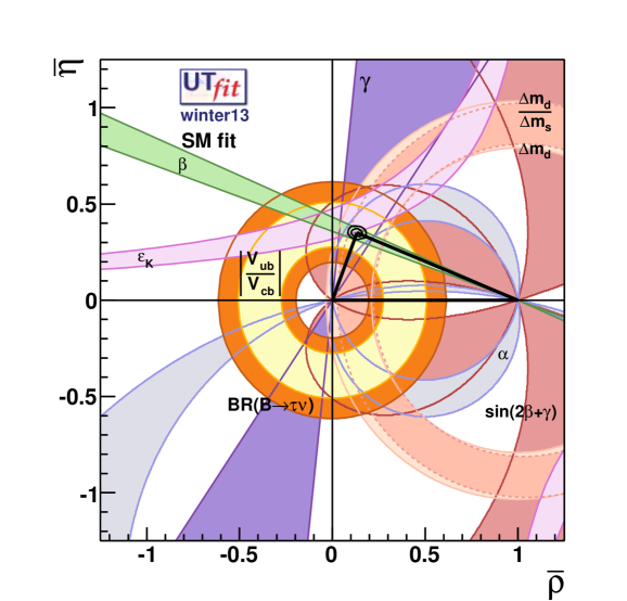
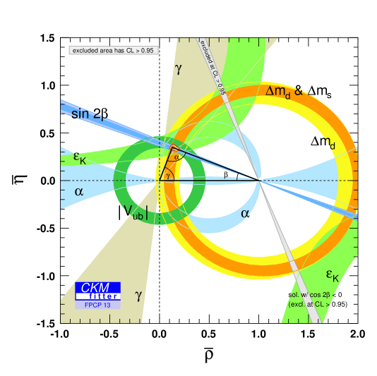
Figure 4.2: Unitarity triangles in the $\overline{\varrho}-\overline{\eta}$ plane from the UTfit [135] (top) and CKMfitter [136] (bottom) collaborations.

The plots from figure 4.2 illustrate the constraints in the $\overline{\varrho}-\overline{\eta}$ plane from various measurements and the global fit result. The shaded 95% CL regions are shown and one can see that they all overlap consistently around the global fit region, leaving not many space for new physics.

For completeness, we review in the following how the angles of the triangle are obtained (see for instance [138] about this topic).

The angle $\alpha$ is obtained from charmless hadronic $B$ decays. This angle can not be measured directly, it should be extracted from measurements where other penguin diagrams not related with $\alpha$ appear. This is done for example in the $B\rightarrow\pi\pi$ system, as explained in [139], by measuring six different quantities related with the three processes $B^{0}\rightarrow\pi^{+}\pi^{-}$, $B^{0}\rightarrow\pi^{0}\pi^{0}$, and $B^{+}\rightarrow\pi^{+}\pi^{0}$ and then, by using the approximate isospin symmetry, combining them to extract the angle. From the decays $B\rightarrow\rho\rho$ and $B^{0}\rightarrow\rho^{0}\pi^{0}$ it can be also extracted, using basically the same method.

The angle $\gamma$ is one of the parameters of the fit known with less precision. It can be obtained from tree dominated decays $B\rightarrow DK$. These measurements have the advantage of having almost zero theoretical uncertainty when the hadronic parameters needed are also obtained from the data. The main techniques for measuring $\gamma$ are the GWS method [140, 141] using $D^{0}$ decays to ${\cal CP}$ eigenstates, the ADS method [142, 143] similar but where the ${\cal CP}$ asymmetry between the amplitudes involved is larger than in the last method, and the Dalitz plots analyzes used for example by Belle in [144] being the precision on the angle dominated by these last ones.

The angle $\beta$ can be obtained directly by $b\rightarrow c\bar{c}s$ decays (as $B^{0}\rightarrow{J\mskip-3.0mu/\mskip-2.0mu\psi\mskip 2.0mu}K^{0}_{S}$) or by $b\rightarrow q\bar{q}s$ penguin-dominated decay modes. The first ones are theoretically and experimentally very clean channels. These have been measured for example by LHCb [145] (the most precise measurement of $\sin 2\beta$ at a hadron collider) or Belle [146]. The seconds have been measured for example by BaBar [147]. The measurement of $\sin 2\beta$ has been dominated by the $B$ factories, but it is currently being matched by the LHCb.

In summary, the current values of the CKM elements, obtained from a global fit using all the available measurements and imposing the SM constraints, are collected in the following matrix [118]:

$$V_{\rm CKM}=\left(\begin{array}[]{ccc}0.97427\pm 0.00015&0.22534\pm 0.00065&0.00351^{+0.00015}_{-0.00014}\\ 0.22520\pm 0.00065&0.97344\pm 0.00016&0.0412^{+0.0011}_{-0.0005}\\ 0.00867^{+0.00029}_{-0.00031}&0.0404^{+0.0011}_{-0.0005}&0.999146^{+0.000021}_{-0.000046}\end{array}\right).$$ (4.30)

4.1.2 Flavour in the lepton sector

The SM considers the neutrinos as massless particles, and all SM interactions preserve Lepton Flavour number. Therefore the SM predicts zero rates for all the Lepton Flavour Violating (LFV) processes to all orders in perturbation theory. However we know from experiments that the Lepton Flavour number is violated in the neutrino sector since the neutrinos oscillate, and thus models of new physics beyond the SM should be proposed to generate neutrino masses and oscillations in flavour to be in agreement with data.

The small mass of the neutrinos could be generated by introducing right-handed neutrinos (sterile neutrinos, without gauge interactions) and by adding small Dirac (via tiny neutrino Yukawa couplings) or/and Majorana mass terms in the Lagrangian, but then a new problem of fine-tuning appears, since these terms should produce unnaturally small values for the mass of the neutrinos. There are mechanisms that solve this issue as for instance the seesaw mechanism [148, 149, 150, 151, 152, 153, 154, 155, 156, 157, 158, 159, 160, 161, 162]. The seesaw mechanism introduces two different natural mass scales: a very heavy Majorana mass $m_{M}$ from the high energy scale theory (usually set at $m_{M}\sim{\cal O}(10^{14}-10^{15}GeV)$) and a Dirac mass of the order of the electroweak scale ($m_{D}\sim Y_{\nu}\langle\phi\rangle$), that produce then very heavy (at the $m_{M}$ scale) and very light (at or below the eV scale) neutrinos in the final mass basis. However, for the purpose of the present work, we will not assume any particular model nor mechanism for neutrino mass generation.

About the LFV processes, they have been observed only in neutrino oscillations, but not in charged leptons. When extending the SM to include neutrino masses and neutrino mixings in agreement with the observed experimental values [163], LFV processes with external charged leptons of different generations can then occur via one-loop diagrams with neutrinos in the internal propagators, but the predicted rates are extremely tiny, far from being in the foreseeable future reachable experimentally, due to the small masses of the neutrinos. Therefore, a potential future measurement of any of these (charged) LFV processes will be a clear signal of new physics and will provide interesting information on the involved flavour mixing, as well as on the underlying origin for this mixing (for a review see, for instance, [164]). Thus, LFV processes provide one of the most challenging probes to physics beyond the SM of particle physics, and in particular to new physics involving non-vanishing flavour mixing between the three generations. In the rest of this work, we will use the term LFV to refer specifically to the charged lepton flavour violating processes, as it is common in the literature.

Without focusing in any particular model to produce the neutrino masses and mixings, that is beyond the scope of this work, we know from the experiments where $\nu$ oscillations have been assumed that the neutrinos get rotated from the interaction basis to the mass basis with a matrix equivalent to the CKM matrix of the quark sector, called here the Pontecorvo-Maki-Nakagawa-Sakata (PMNS) matrix [26, 27, 28], whose values will be summarized below.

The mass states of the neutrinos get rotated to the flavour states by the PMNS matrix [26, 27, 28] as follows:

$$\nu^{\rm int}_{L}=V_{\rm PMNS}\nu^{\rm phys}_{L}$$ (4.31)

This matrix is usually parametrized in terms of 3 mixing angles $\theta_{12}$, $\theta_{13}$ and $\theta_{23}$, and 1 or 3 phases depending if the neutrinos are Dirac or Majorana fermions respectively:

$$V_{\rm PMNS} = \left(\begin{array}[]{ccc}V_{e1}&V_{e2}&V_{e3}\\ V_{\mu 1}&V_{\mu 2}&V_{\mu 3}\\ V_{\tau 1}&V_{\tau 2}&V_{\tau 3}\end{array}\right)$$ (4.35)

$$= \left(\begin{array}[]{ccc}c_{12}c_{13}&s_{12}c_{13}&s_{13}e^{-i\delta}\\ -c_{12}s_{23}s_{13}e^{i\delta}-s_{12}c_{23}&-s_{12}s_{23}s_{13}e^{i\delta}+c_{12}c_{23}&s_{23}c_{13}\\ -c_{12}c_{23}s_{13}e^{i\delta}+s_{12}s_{23}&-s_{12}c_{23}s_{13}e^{i\delta}-c_{12}s_{23}&c_{23}c_{13}\end{array}\right)\left(\begin{array}[]{ccc}1&0&0\\ 0&e^{i\frac{\alpha_{21}}{2}}&0\\ 0&0&e^{i\frac{\alpha_{31}}{2}}\\ \end{array}\right).$$ (4.42)

where $s_{ij}=\sin\theta_{ij}$, $c_{ij}=\cos\theta_{ij}$, the angles $\theta_{ij}$ go from 0 to $\pi/2$ and the phases from 0 to $2\pi$. $\delta$ is the Dirac ${\cal CP}$ violation phase, and $\alpha_{ij}$ the Majorana ${\cal CP}$ violation phases. We are using here the same notation for the mixing angles and delta as in the quark case, but they should obviously not been confused. Notice also that, in contrast to the quark case where flavour states refer to the mass states, in the case of neutrinos flavour states refer to the interaction states. The other important parameters are the mass differences, as we will see later. Only two of the mass squared differences are independent parameters, that will be taken as $\Delta m_{21}^{2}$ and $\Delta m_{31}^{2}$. We will not enter here in the description of the topics related with the absolute value of the masses.

The mixing between neutrino flavours that imply the PMNS matrix has been observed experimentally through the neutrino oscillations in solar, atmospheric, accelerator and reactor neutrinos [165, 166, 167, 168, 169, 170, 171, 172, 173, 22, 174, 175, 176]. Neutrinos produced by one of these sources in a specific flavour state are found in another state at a certain distance. As the distance is varied, the proportion of neutrinos in each flavour oscillates. The oscillation is produced by the fact that, as we have already said, the flavour states are not mass states (eigenstates of the Hamiltonian), and therefore evolve differently in time. Depending on the source the initial flavour state is different: solar ($\nu_{e}$), atmospheric ($\nu_{\mu}$, $\bar{\nu}_{\mu}$), accelerator ($\nu_{\mu}$) and reactor ($\bar{\nu}_{e}$) neutrinos. The probability of transition of the initial neutrinos after some distance depends mainly on the elements of the PMNS matrix, the mass differences between the mass states, the energy of the neutrinos produced and the distance at which the measurement is done. And the transitions happen only if at least two neutrinos are not degenerate and the mixing angles are not zero. Since the value of $V_{e3}$ is small, the mass and mixing angles related with the transitions “12” and “23” are responsible respectively of the transitions of the solar and atmospheric neutrinos, and is common to label them with these words (e.g. $\theta_{23}=\theta_{atm}$). It is also common to study the oscillations just considering the two main flavours involved on it, to simplify the equations.

The transition probability between two different flavours $l$ and $l^{\prime}$ is given by [177]:

$$P(\nu_{l}\rightarrow\nu_{l^{\prime}})=\sum_{j}|V_{l^{\prime}j}|^{2}|V_{lj}|^{2}+2\sum_{j>k}|V_{l^{\prime}j}V_{lj}^{*}V_{lk}V_{l^{\prime}k}^{*}|\cos(\frac{\Delta m_{jk}^{2}}{2p}L-\phi_{l^{\prime}l;jk})$$ (4.43)

where $\phi_{l^{\prime}l;jk}={\rm arg}(V_{l^{\prime}j}V_{lj}^{*}V_{lk}V_{l^{\prime}k}^{*})$, and the result is the same for $P(\bar{\nu}_{l}\rightarrow\bar{\nu}_{l^{\prime}})$ just changing the sign of $\phi_{l^{\prime}l;jk}$.

When considering just two flavours in the transition: $|\nu_{l}\rangle=\cos\theta|\nu_{1}\rangle+\sin\theta|\nu_{2}\rangle$ and $|\nu_{l}^{\prime}\rangle=-\sin\theta|\nu_{1}\rangle+\cos\theta|\nu_{2}\rangle$, the previous equation gets simplified to:

$$P^{2\nu}(\nu_{l}\rightarrow\nu_{l^{\prime}})=\frac{1}{2}\sin^{2}2\theta(1-\cos\frac{\Delta m^{2}L}{2p})$$ (4.44)

where $\Delta m^{2}=m^{2}_{2}-m^{2}_{1}>0$, and it is often defined the oscillation length $L_{0}=4\pi p/\Delta m^{2}$.

Then setting experiments at the appropriate distances (related with the energy of the neutrinos produced) the transitions can be observed, and the angles obtained. As an example see Figure 4.3 where in the left plot we see the probability of finding a muon neutrino of a given energy at distance $L$ after it is produced: $P^{2\nu}(\nu_{l}\rightarrow\nu_{l})=1-P^{2\nu}(\nu_{l}\rightarrow\nu_{l^{\prime}})$. In the right plot we find the same probability for detecting neutrinos with energy spread around the previous value.

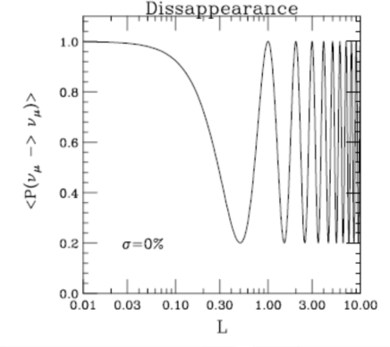
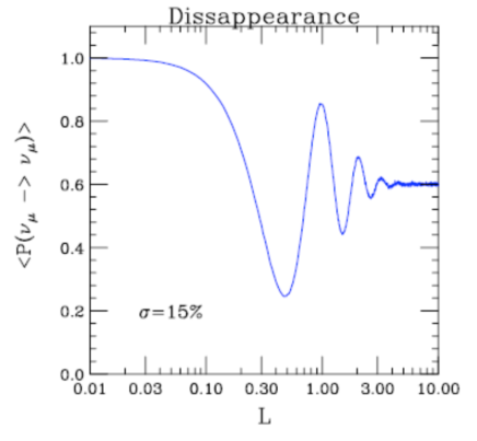
Figure 4.3: Probability of finding muon neutrinos at distance $L$ after they are produced for two flavours with a mixing angle around 0.55, for neutrinos with a given energy that fulfils $L_{0}=1$ (left) or with energies spread around the previous value (right). Plots from [178]

The previous equations are valid for neutrino oscillations in vacuum. When neutrinos are travelling through matter, it has an effect over them and modifies the transition probabilities. The incoherent elastic scattering (the state after the scattering is not the same as the initial one) and quasielastic scattering (the energy transferred to the medium through the scattering is small) with the matter are processes not relevant to the neutrino transitions observed. The scattering for the $\nu_{\mu}\leftrightarrow\nu_{\tau}$ transition produces also negligible effects through the Sun and the Earth [179]. We are just left with the coherent elastic scattering for the $\nu_{e}\leftrightarrow\nu_{\mu,\tau}$ transition. This process produce differences in the refraction indices of the neutrinos involved, and the effect modifies the Equation 4.44 changing $\theta$ and $L_{0}$ for $\theta_{m}$ and $L_{m}$ (see equations in [177]) that are related to the previous values and the density of electrons in the matter. These effects are important and should be taken into account for the experiments.

$\boldsymbol{\theta_{12}}$ and $\boldsymbol{\Delta m_{12}}$. Solar neutrinos have been observed in different experiments by the interaction of the neutrinos with the medium of the experiment: Homestake, SAGE, GALLEX, GNO, Kamiokande and Super-Kamiokande, Borexino and SNO. In Homestake the neutrinos transmuted chlorine into radioactive argon whose decay was then observed; SAGE, GALLEX and GNO observed the transformation of gallium into germanium; Kamiokande and Super-Kamiokande observed the Cherenkov light produced by the scattering between the neutrinos and the electrons of the water contained in the detector (with the advantage of being able of measuring the direction, and hence the origin of the Sun); Borexino detected that last scattering in a mixture of ultra pure liquid scintillator; SNO observed the interaction of the neutrinos with deuterium, producing electrons or neutrons.

The calculation of the number of neutrinos produced by the Sun is done through the standard solar model (see for instance [180, 181, 182] and references in [183]). What at the beginning of the observations was called the solar neutrino problem, as the Sun produced less neutrinos than what was expected, was resolved by the neutrino oscillations. The SNO experiment, different to the other commented, was sensitive not only to electron neutrinos but to all flavours. This feature, combined with the precision measurement by the other experiments, especially Super-Kamiokande, confirmed the flavour oscillation [172, 173, 184, 185]]. These observations were combined with the data from the KamLAND experiment, to obtain the best values for the mixing angle and the mass difference [186]. The KamLAND experiment is a liquid scintillator detector situated underground, in the same mine as Kamiokande, to reduce the effects from cosmic rays. KamLAND, instead of solar neutrinos, measured the well known flux from antineutrinos coming from nuclear reactors situated at a distance around 100 Km. KamLAND not only contributed to measure the flavour transition, but was able to observe the oscillation as the ratio distance/energy varied [176, 187, 186].

$\boldsymbol{\theta_{23}}$ and $\boldsymbol{\Delta m_{23}}$. The oscillation of atmospheric neutrinos was observed first by Super-Kamiokande [22]. The experiment detected muon and electron neutrinos from the zenith angle, and observed how part of the muon neutrinos travelling trough the Earth disappeared (presumably oscillating into tau neutrinos), while that was not happening for the muon neutrinos from above. This effect was not present for the electron neutrinos. The hypothesis was confirmed by long-baseline experiments observing neutrinos from accelerators like K2K (KEK-to-Kamioka) [188] and MINOS [189]. The first produced neutrinos in the KEK-PS accelerator situated 250 Km away from the detector, with a mean energy of 1.3 GeV; and the second in the NuMI facility at Fermilab, 753 Km away, with a variable energy around 17 GeV.

$\boldsymbol{\theta_{13}}$. After many years having only bounds, finally in the last years some experiments have been able to measure $\theta_{13}$. These are Double Chooz [190], Daya Bay [191] and RENO [192]. The three studied $\bar{\nu}_{e}$ disappearance from reactors by using liquid scintillators.

The current experimental values for the angles and the mass differences, as obtained from [193], can be found in table 4.2.

Parameter	Best fit value	$3\sigma$ range
$\Delta m^{2}_{12}$	$7.54\times 10^{-5}$ eV2	$(6.99,8.18)\times 10^{-5}$ eV2
$\Delta m^{2}(NH)$	$2.43\times 10^{-3}$ eV2	$(2.19,2.62)\times 10^{-3}$ eV2
$\Delta m^{2}(NH)$	$2.42\times 10^{-3}$ eV2	$(2.17,2.61)\times 10^{-3}$ eV2
$\sin^{2}\theta_{12}$	$3.07\times 10^{-1}$	$(2.59,3.59)\times 10^{-1}$
$\sin^{2}\theta_{23}(NH)$	$3.86\times 10^{-1}$	$(3.31,6.37)\times 10^{-1}$
$\sin^{2}\theta_{23}(IH)$	$3.92\times 10^{-1}$	$(3.35,6.63)\times 10^{-1}$
$\sin^{2}\theta_{13}(NH)$	$2.41\times 10^{-2}$	$(1.69,3.13)\times 10^{-2}$
$\sin^{2}\theta_{13}(IH)$	$2.44\times 10^{-2}$	$(1.71,3.15)\times 10^{-2}$

Table 4.2: Current experimental values for the angles and the mass differences of the PMNS matrix as obtained from [193]. $\Delta m^{2}=|m_{3}^{2}-\frac{m_{1}^{2}+m_{2}^{2}}{2}|$ according to[194]. Values valid for normal hierarchy (NH) or inverted hierarchy (IH) when stated.

4.2 Experimental searches of rare processes in flavour physics

The most important experiments at the moment with respect to the flavour changing processes in the quark sector are the $B$ factories and the LHCb. There are also important searches related to the first and second generation, but these mixings are very restricted by the past century experiments leaving not much space for new physics, that is why we will pay more attention here to the third generation. These experiments focus mainly in $B$ physics observables which turn out to be very good laboratories for the search of new physics. With respect to the study of LFV processes, besides the previously commented, there are MEG, SINDRUM II, and some other proposed experiments as COMET, Mu2e or PRISM.

Belle [60] is an experiment situated in the KEKB $e^{+}e^{-}$ collider in Tsukuba (Japan). The first version run from 1999 to 2010 and collected over 1000 fb^-1 of data. It was designed for the observation of time-dependent ${\cal CP}$ violation in $B$ mesons, but it was able of conducting important researches in other topics, specially, but not only, in $B$ physics. Other topics covered were hadron spectroscopy, two-photon physics and $\tau$ physics. A review of Belle achievements can be found in [195]. Most of the data was obtained with a luminosity around the $\Upsilon(4S)$ resonance, that is the best energy for the production of $B\bar{B}$ pairs (the $\Upsilon$ meson is formed by a b quark and its antiquark).

Measuring the decay rates and asymmetries between the decays of the two $B$ mesons for the different modes, it was possible to measure the different angles of the unitarity triangle. The decays used are the ones explained in the end of the section above. The equations for the rates and asymmetries can be found in [195]. The first angle to be measured was $\beta$ and then $\alpha$ was obtained. This second angle was more difficult to be measured due to theoretical uncertainties from the contributions of penguin diagrams. The last studies of $\alpha$ using the full data set are: [196] from $B\rightarrow\pi\pi$ and from $B\rightarrow\rho^{0}\rho^{0}$ is [197]. $\gamma$ was theoretically clean using only tree-level processes, but needed much more data than the other two. The last value for $\gamma$ from Belle can be found in [198].

$b\to s$ decays mediated by penguins were studied in Belle, searching for new physics inside the loops. For example, there were checked $b\to s\bar{q}q$ induced decays as $B^{0}\to\eta^{\prime}K^{0}_{S}$ and $B^{0}\to\phi K^{0}_{S}$. Other processes studied were $B^{-}\to\ell^{-}\bar{\nu}_{\ell}$. These can be measured with high precision, and also calculated with high precision in the SM, so they are a good place to look for new physics. The calculation involves the parameter $f_{B}$ that has to be calculated by lattice QCD, so it is also a good test of it. Other interesting decay studied looking for new physics was $B\to D^{(*)}\tau\nu$, a channel that gave interesting results in BaBar.

Rare $B$ decays have also been studied to probe new physics beyond the SM. $B$ decays into hadrons not containing charm quarks are a good example. These are very suppressed in the SM, by the CKM elements (in the decays to the u quark) or by penguins (in the rest of the decays), and thus they are very interesting. Also radiative penguin decays as ${\rm BR}(B\to X_{s}\gamma)$, or electroweak penguin decays as $b\to s(d)l^{+}l^{-}$, not allowed at tree level in the SM, have been observed. ${\rm BR}(B\to X_{s}\gamma)$ has been studied not only inclusively, but exclusively through channels like $B\to K\rho\gamma$, $B\to K\phi\gamma$ and $B\to K\pi\gamma$. These are promising modes for the next phase of the experiment. The inclusive measurement of $b\to sl^{+}l^{-}$ is not easy experimentally, but the theoretical prediction is clean. In general these decays suffer from large theoretical uncertainties, so it is common to measure ratios or asymmetries to eliminate them. These decays will be studied in the next sections in more detail, where we will see their potential to find new physics.

Tau physics has been another topic explored in Belle. The main issues studied were lepton flavour violating decays, ${\cal CP}$ violation in the charged lepton sector, the electric dipole moment of the $\tau$, and SM precision measurements. Tau physics is interesting since it is the only lepton whose mass allow it to decay into hadrons, and then is possible to study QCD with a cleaner system. The large mass of the tau also allows it to decay in many different LFV decays. Belle has studied 46 LFV tau decay modes using the whole set of data and found no evidence of it. LFV physics will be studied in detail in the following chapters. Two of the decays considered in our study $\tau\rightarrow\mu\gamma$ and $\tau\rightarrow e\gamma$ were studied in Belle [199] looking for opposite $\tau^{+}\tau^{-}$ pairs, that decay to the searched decay in one side (the signal-side) with an invariant mass of the $\tau$ particle, and to a SM decay in the other side (the tag-side). It was also studied $\tau\rightarrow lll$ [200]. Other LFV searches are for example in [201].

The measurements of Belle are consistent with the SM, leaving around a 10% of space beyond the SM amplitudes allowing for new physics.

The next phase of Belle is called Belle-II [63, 64], and will be running in the SuperKEKB collider, starting with the physics in 2016. The luminosity at this Super-$B$ factory is $8\times 10^{35}$cm^-2s^-1, 50 times the peak luminosity achieved in KEKB. This corresponds to an annual integrated luminosity of 8 ab^-1 assuming 100 days of operation. A review about the physics in this Super-$B$ factory can be read in [202].

The BaBar experiment [61] operated in the asymmetric $e^{+}e^{-}$ collider PEP-II at the SLAC National Accelerator Laboratory in California (USA). The PEP-II collider worked from 1999 to 2008. Designed to study the ${\cal CP}$ violation, BaBar worked at a centre of mass energy equal to the mass of the $\Upsilon(4S)$ resonance, as Belle. Apart from ${\cal CP}$ violation and the test of the CKM model, it produced interesting research on other fields as $\tau$ physics, heavy quarks physics, including bottomonium (bound states formed by a b quark and an anti-b) and charmonium physics, $D$ mesons decays and new physics searches.

The chosen $\Upsilon(4S)$ resonance is a good choice in terms of signal to background ratio. The only problem is that the $B\bar{B}$ pairs created from its decay are created with very low momenta in the frame of the resonance, and hence time-dependent measurements are difficult. The asymmetric energy of the $e^{+}$ and $e^{-}$ beams produces a large boost of the resonance with respect to the laboratory frame, solving this problem.

The peak luminosity of PEP-II was $1.2\times 10^{34}$cm^-2s^-1. BaBar collected 430fb^-1 of data around the $\Upsilon(4S)$ resonance.

The angles of the unitarity triangle were measured in BaBar, by the decays explained at the end of the subsection 4.1.1.2. The study of $\alpha$ using the full data set from the $B\rightarrow\pi\pi$ decay can be found in [203]. The last value of $\gamma$ also with the whole collection of data was published in [204]. The angles show good consistency with the SM.

${\cal CP}$ violation was confirmed in BaBar, and following the CPT theorem, this implies ${\cal T}$ violation. However this last is more difficult to be seen directly. As an example, ${\cal CP}$ violation was observed in the $B\to K\pi$ decay, but the ${\cal T}$ reverse decay $K\pi\to B$ that should be observed to measure the asymmetry was impossible to observe. It was not possible to prepare the initial state $K\pi$, and hadronic interactions would make difficult in any case to observe the asymmetry. However, a method was proposed by Bernabeu et al. [205, 206], using the entanglement of the two $B$ mesons produced from the $\Upsilon(4S)$ resonance. This ${\cal T}$ violation was finally observed in BaBar [207] with a significance equivalent to $14\sigma$.

Two interesting channels studied in BaBar were $B\to D^{(*)}\tau\nu$ and $B\to\tau\nu$. These are tree level decays mediated by a $W^{\pm}$ in the SM, so it could be mediated by a charged Higgs in the case of the MSSM. Thus the branching fractions, and the kinematic distributions (in the first decay) are sensitive to an enlarged Higgs sector as the one in the MSSM. The decay $B\to\tau\nu$ was measured [208], and it was found to reach a $2.4\sigma$ discrepancy with the SM. The decay $B\to D^{(*)}\tau\nu$ was also measured [209] and the results were $3.4\sigma$ higher than in the SM. The combination of the last data of Belle with the data of BaBar, shown in [210], enlarge the discrepancy with the SM to $4.8\sigma$. New results and analysis of data are awaited for confirmation. Other interesting rare decays as ${\rm BR}(B\to X_{s}\gamma)$ were also measured [211].

With respect to LFV, $B$ factories are $\tau$ factories too: $\sigma(e^{+}e^{-}\rightarrow\tau^{+}\tau^{-})\approx\sigma(e^{+}e^{-}\rightarrow b\bar{b})$, so it is interesting to study the tauonic channel (also for the large $\tau$ mass compared with other leptons, that increase some branching ratios). In BaBar, as in Belle, LFV decays were studied as for example the ones that will be studied in this work $\tau\rightarrow\mu\gamma$ and $\tau\rightarrow e\gamma$ [212], and $\tau$ in three leptons [213]; and also other decays as the ones in [214]

The LHCb experiment [62] is a forward spectrometer located at the LHC collider, aimed to study heavy flavour physics. Its main object is to study ${\cal CP}$ violating observables and rare decays. It is designed to use the decays of b and c hadrons to obtain its measurements. In the LHC there are produced pairs of b and anti-b quarks, basically via gluon fusion, gluon splitting and flavour excitation. These pairs are produced mainly in the forward or backward direction, being this the reason for the chosen design of the experiment. The acceptance of the detector is for particles with a pseudorapidity between 2 and 5.3. The experiment is designed to operate at a luminosity of $4\times 10^{32}$cm^-2s^-1, lower than the nominal luminosity of the LHC, and the one used for the two main general detectors. This decrease is produced by reducing the overlap between the beams. Until the moment, the detector collected 3 fb^-1 of data.

Between the observations of the LHCb one can find the ${\cal CP}$ violation in the decays of $B^{0}_{s}$ mesons [215], never observed before, the study of $B^{0}\to K^{*0}\mu^{+}\mu^{-}$ [216], and the most precise measurement to date of $B^{0}_{s}$-$\bar{B}^{0}_{s}$ mixing [217], an important observable for our present work that will be studied in next chapters with more detail.

One of the last successes of the LHCb (together with CMS) was the measurement of $B^{0}_{s}\to\mu^{+}\mu^{-}$ [218]. The value obtained was compatible with the SM. This observable is very relevant. It is highly suppressed in the SM, similarly to other FCNC process and also being helicity suppressed (because of the structure of the interaction, to conserve the helicity some final helicity states are suppressed), so it is a good probe for possible new physics, and it has a very precise measurement in the SM. It is sensitive to scalar and pseudoscalar contributions of new theories. It has direct implications in the MSSM space of parameters, and therefore will be used through this work as one of our reference observables. The experiment also gave bounds on $B^{0}_{(s)}\to\mu^{+}\mu^{-}\mu^{+}\mu^{-}$ [219] and also in the LFV observable $B^{0}_{(s)}\rightarrow e^{\pm}\mu^{\mp}$ [220]. With respect to charm physics, LHCb presented bounds to $D^{0}\to\mu^{+}\mu^{-}$ [221], also a FCNC helicity suppressed observable, and to $D^{+}\to\pi^{\pm}\mu^{+}\mu^{\mp}$ [222], giving the world best upper limits to all of them.

The study of the $\tau$ decays has some disadvantage in the LHCb as compared to the $B$ factories, not being able to do $\tau$ tagging, however the inclusive $\tau$ cross section is much larger, $79.5\pm 8.3\mu b$ in LHCb as compared with 0.919 nb in the $B$ factories, compensating the former fact. Rare $\tau$ decays have been explored as $\tau\rightarrow\mu\mu\mu$ [223] or the ones of [224] and [220].

The next upgrade of the LHCb in 2018 [65] will allow to carry on precision studies on flavour. For example, it will be possible to determine $B^{0}_{s}\to\mu^{+}\mu^{-}$ down to a 10% of the SM value, to measure the CKM angle $\gamma$ with an error smaller than 1 degree, or search ${\cal CP}$ violation in charm below the $10^{-4}$ level. Some expected values for the precision of different observables can be found in [65].

  

MEG [59] is an experiment located at the Paul Scherrer Institute (PSI) in Switzerland, optimized to detect the decay $\mu^{+}\rightarrow e^{+}\gamma$. It consists in an intense positive muon beam of $3\times 10^{7}\mu^{+}/s$, that is stopped at a thin target inside of COBRA, a superconducting magnet, aiming to produce positrons with an helicoidal trajectory and a signal in the drift chamber, and photons that would be detected in a liquid Xenon scintillator detector outside of the magnet.

The experiment has been running since 2008, with for example $22\times 10^{22}$ stopped muons during 2012, and has produced the best bound in the world for the searched decay [225] ${\rm BR}(\mu\to e\gamma)<5.7\times 10^{-13}$. An upgrade is proposed [226] with a goal of reaching a sensitivity of $6\times 10^{-14}$. In Chapter 8 will be studied this decay and the predictions of SUSY for it.

The research of rare $\mu$ decays by this experiment in PSI was the continuation of the SINDRUM II experiment. This detector was a magnetic solenoidal spectrometer designed to search for $\mu-e$ conversion in nuclei, holding the current best bound for the conversion in Gold ${\rm CR}(\mu-e,{\rm Au})<7.0\times 10^{-13}$ [227]. The muons were produced by a 590 MeV beam of protons hitting a carbon target. Inside the spectrometer was located the gold target that was hit by the muons. More details about the experiment can be found on [227] and [228].

The next future experiments for studying rare $\mu$ decays are COMET and Mu2e. COMET [66] will be located in Tokai in Japan and will use the J_PARC proton beam. It will study the $\mu-e$ conversion in aluminium atoms with a sensitivity of $10^{-17}$ at 90% CL in the second phase. The first physics run of phase-I is due to 2017 and the second phase physics run in 2021. Mu2e [67, 68] will be located in Fermilab and will study the same conversion with the same sensitivity as COMET. The initial preliminary results are expected in 2021. After them, the next experiment designed is PRISM [69]. PRISM will use a fixed-field alternating gradient accelerator [229] for rendering monochromatic the muon beam obtained as in COMET. Having all the muons with the same energy will exploit the sharpness of the peak in the energy distribution of the electron decay, improving the signal/background ratio. It could improve the sensitivity of COMET until $10^{-18}$. Another proposed experiment is Mu3e [230, 231], also in PSI, whose aim is to measure the decay $\mu\rightarrow eee$ with an expect sensitivity of $10^{-15}$ and $10^{-16}$ in the first and second phases respectively.

Finally, for our selected particular LFV processes of relevance in the present work, we have collected a summary of their present bounds in the forthcoming Section 8.1.3.

4.3 The flavour of new physics

In the previous section, we have seen how the flavour physics is a good window for the search of new physics. In the next sections we will shortly comment on some techniques and hypothesis related with the searches of new physics beyond the Standard Model in flavour observables, and in particular for the searches of SUSY in mesonic observables.

4.3.1 The effective Hamiltonian approach and the scale of new physics

Using the full supersymmetric theory for doing predictions is a difficult task for $B$ physics observables so we will use an easier way to attack the problem: the method of the Operator Product Expansion (OPE). The OPE is a way to Taylor expand the Hamiltonian of the theory in what are called effective Hamiltonians, and perform the predictions using the most relevant terms until some order. The processes we are interested in involve different energy scales, the idea behind the expansion is working with a Hamiltonian with the degrees of freedom of the energy of the process, where the high energy degrees of freedom have been integrated out and their effects are collected in some coefficients. These coefficients are calculated at high energy, and they are evolved to the low energy using the proper Renormalization Group Equations. We comment briefly on this expansion in the following:

Our goal is to calculate an approximation to the $S$ matrix element between some general initial and final states $\langle F|S|I\rangle$ using the full theory. Instead of the full Hamiltonian we will use an effective Hamiltonian:

$${\cal H}_{W}=4\frac{G_{F}}{\sqrt{2}}\sum_{i}C_{i}(\mu)O_{i}(\mu)$$ (4.45)

where $G_{F}$ is the Fermi constant $G_{F}/\sqrt{2}=g^{2}/8M_{W}^{2}$, the $C_{i}$ are called Wilson coefficients, and $O_{i}$ are the low energy local operators, both renormalized at a scale $\mu$. To satisfy our goal it should be fulfilled the following relation:

$$\langle F|iS|I\rangle=4\frac{G_{F}}{\sqrt{2}}\sum_{i}C_{i}(\mu)\langle F|O_{i}(\mu)|I\rangle+\dots\,,$$ (4.46)

The terms of the expansion not shown are suppressed by inverse powers of the high energy scale, the scale where the full theory operates.

The operators $O_{i}$ are a complete basis of the OPE, containing all the operators producing the transition between $I$ and $F$, with the proper dimensions and the same quantum numbers as the original element of the full theory that connects the two states, and respecting all the symmetries of the full theory. One must also take into account that when running the RGE to low energy, new operators can be generated to add to the first set.

Once the basis of operators is obtained, one has to obtain the Wilson coefficients. This is done by first “matching” the value of the amplitudes at high energy using the full theory and the effective Hamiltonian (up to terms suppressed by inverse powers of the high energy scale) as in Eq. 4.46, and second running the RGE from the matching scale down to the renormalization scale $\mu$. The Wilson coefficients then encode (and depend only on) the information of the high energy (low distances) physics, and act as effective couplings in our new Hamiltonian.

Once the coefficients and operators are obtained, one can calculate the transition between the two chosen states. For that one has to calculate matrix elements of the new operators between the states. For transitions between hadronic states as the ones we are interested in this work, this has to be done by non-perturbative methods as lattice QCD, or they have to be measured in some process and then used the obtained values for other processes.

When understanding the SM as an effective theory, one can study the effects of physics beyond the SM by using higher dimensional operators not contained in the SM. These operators are suppressed by inverse powers of the scale of the new physics. As the SM predictions match better the experiments, the space for these new operators get reduced, meaning in general terms, moving away the new physics scale to higher energies.

For example, one can check the scale for new physics from the amplitudes of meson-antimeson mixings as $K^{0}$–$\overline{K^{0}}$, $B_{d}$–$\overline{B}_{d}$, and $B_{s}$–$\overline{B}_{s}$. The amplitudes of these $\Delta F=2$ transitions, where the quark flavour quantum numbers change by two units, go in the SM approximately as

$$\mathcal{A}_{\rm SM}^{\Delta F=2}\approx\frac{G_{F}^{2}m_{t}^{2}}{16\pi^{2}}\left(V_{ti}^{*}V_{tj}\right)^{2}\times\langle\overline{M}|(\overline{Q}_{Li}\gamma^{\mu}Q_{Lj})^{2}|M\rangle\times F\left(\frac{M_{W}^{2}}{m_{t}^{2}}\right),$$ (4.47)

where $F$ is a loop function of $\mathcal{O}(1)$, $V_{ij}$ are the CKM elements and $Q_{Li}$ are the corresponding quarks involved.

One can compare this with the amplitude produced by the new physics (NP) effective operators

$$\Delta\mathcal{L}^{\Delta F=2}=\sum_{i\not=j}\frac{c_{ij}}{\Lambda^{2}}(\overline{Q}_{Li}\gamma^{\mu}Q_{Lj})^{2}~{},$$ (4.48)

where the $c_{ij}$ are dimensionless couplings and $\Lambda$ is the new physics scale.

As shown in [232], the condition $|\mathcal{A}^{\Delta F=2}_{\rm NP}|<|\mathcal{A}^{\Delta F=2}_{\rm SM}|$ can be translated into lower bounds on the new physics scale

$$\Lambda>\frac{4.4~{}{\rm TeV}}{|V_{ti}^{*}V_{tj}|/|c_{ij}|^{1/2}}\sim\left\{\begin{array}[]{l}1.3\times 10^{4}~{}{\rm TeV}\times|c_{sd}|^{1/2}\!\!\!\!\!\!\!\\ 5.1\times 10^{2}~{}{\rm TeV}\times|c_{bd}|^{1/2}\!\!\!\!\!\!\!\\ 1.1\times 10^{2}~{}{\rm TeV}\times|c_{bs}|^{1/2}\!\!\!\!\!\!\!\end{array}\right.$$ (4.52)

Therefore, in order to have the new physics at $\Lambda$ reachable by the present experiments the couplings $c_{ij}$ of the new operators connecting flavours of different generations should be very small, as seen in the last equation. In other words, these imply strong constraints on the flavour mixing coefficients.

The issue that new physics with general flavour structures usually tend to overcome easily the flavour constraints of the experiments is a well known problem. In the literature this problem is usually evaded by assuming the minimal flavour violation hypothesis on the new physics.

4.3.2 The minimal flavour violation hypothesis

The minimal flavour violation hypothesis assumes that the Yukawa couplings (as in the SM) are the only source of flavour violation also in the new physics.

This hypothesis can be studied using the effective field theory approach as before. To do that one first defines the flavour symmetry that is only broken by the Yukawa couplings. This global symmetry, the largest one commuting with the gauge group, would be:

$$G_{\rm Flavour}\equiv{\rm SU}(3)^{3}_{q}\otimes{\rm SU}(3)^{2}_{\ell}\otimes{\rm U}(1)_{B}\otimes{\rm U}(1)_{L}\otimes{\rm U}(1)_{Y}\otimes{\rm U}(1)_{\rm PQ}\otimes{\rm U}(1)_{E_{R}}~{},$$ (4.53)

where

$${\rm SU}(3)^{3}_{q} = {\rm SU}(3)_{Q_{L}}\otimes{\rm SU}(3)_{U_{R}}\otimes{\rm SU}(3)_{D_{R}}~{},$$ (4.54)

$${\rm SU}(3)^{2}_{\ell} = {\rm SU}(3)_{L_{L}}\otimes{\rm SU}(3)_{E_{R}}~{}.$$ (4.55)

The $B$, $L$ and $Y$ charges can be identified with baryon number, lepton number and hypercharge respectively. These three charges are not broken by the Yukawa interactions. The last two ${\rm U}(1)$ charges are a Peccei-Quinn symmetry and a rotation of the right-handed singlets. More details about these groups can be found for instance in [58].

The usual method to implement the MFV hypothesis is to promote the Yukawa couplings as spurions. Instead of parameters, the spurions are defined as (non-physical) fields that transform in the proper way to conserve the symmetry that as parameters they break. They can then be used to construct all the possible symmetric terms of the Lagrangian, and after it they are promoted back to the original parameters, giving us all the possible symmetry breaking terms. In the case of the $G_{\rm Flavour}$ symmetry above, that means Yukawa couplings as fictitious fields transforming as:

$${Y}^{u}\sim(3,\bar{3},1)_{{\rm SU}(3)^{3}_{q}}~{},\qquad{Y}^{d}\sim(3,1,\bar{3})_{{\rm SU}(3)^{3}_{q}}~{},\qquad{Y}^{e}\sim(3,\bar{3})_{{\rm SU}(3)^{2}_{\ell}}~{}.$$ (4.56)

With these dynamical fields the $G_{\rm Flavour}$ symmetry is then satisfied for every higher dimensional operator one can build with these fields in this spurion language, or what is the same, for every operator whose flavour structure is only determined by the Yukawa couplings.

In [58] the possible new physics effective operators using this MFV approach were studied in the one and two Higgs doublets cases, and listed some of them. It is found how the scale of new physics is largely reduced comparing with the general hypothesis we saw before, and stays at $\mathcal{O}(10)$TeV.

The MFV hypothesis can also be applied to supersymmetry, and more specifically to define the structure of the soft SUSY breaking terms that are the terms of the Lagrangian with an unknown flavour structure. This would translate into the following terms [58]:

$$m_{\tilde{Q}}^{2} = {\tilde{m}}^{2}\left(a_{1}1{\rm l}+b_{1}Y^{u}Y^{u\dagger}+b_{2}Y^{d}Y^{d\dagger}+b_{3}Y^{d}Y^{d\dagger}Y^{u}Y^{u\dagger}+b_{4}Y^{u}Y^{u\dagger}Y^{d}Y^{d\dagger}\right)~{},$$ (4.57)

$$m_{\tilde{U}}^{2} = {\tilde{m}}^{2}\left(a_{2}1{\rm l}+b_{5}Y^{u\dagger}Y^{u}\right)~{},$$ (4.58)

$$m_{\tilde{D}}^{2} = {\tilde{m}}^{2}\left(a_{3}1{\rm l}+b_{6}Y^{d\dagger}Y^{d}\right)~{},$$ (4.59)

$${\bar{\cal A}}^{u} = A\left(a_{4}1{\rm l}+b_{7}Y^{d}Y^{d\dagger}\right)Y^{u}~{},$$ (4.60)

$${\bar{\cal A}}^{d} = A\left(a_{5}1{\rm l}+b_{8}Y^{u}Y^{u\dagger}\right)Y^{d}~{}.$$ (4.61)

where $\tilde{m}$ and $A$ are generic SUSY soft mass scales, $a_{i}$ and $b_{i}$ are dimensionless numerical coefficients, and $1{\rm l}$ is the $3\times 3$ identity matrix.

Within the MSSM most of the calculations for flavour observables are done by implementing the MFV hypothesis, therefore by requiring that, as in the SM, the only origin for flavour mixing be the CKM matrix in the quark sector (and the PMNS matrix in the neutrino sector if massive neutrinos are included), and flavour violation is exclusively mediated by the Yukawa interactions.

In the SM, we saw how there were no flavour changing neutral currents at tree level, and the charged currents were mediated by the $W^{\pm}$ bosons (that contributed to the FCNC at loop level). In the MSSM the charged currents are also mediated by the charged Higgs $H^{\pm}$ and the charginos ${\tilde{\chi}}^{\pm}$, that contribute also to the loop-level neutral currents. As we saw before, in the standard sector the FCNC were very suppressed by the GIM mechanism. In the supersymmetric sector, the GIM mechanism will be replaced by a super-GIM mechanism, being the rates for FCNC processes proportional to the ratio between the differences of squared squarks masses and chargino/charged Higgs masses.

In the rest of the work however, we will not use this MFV hypothesis for SUSY but we will assume instead a more general hypothesis, named Non Minimal Flavour Violation (NMFV), where the origin of the flavour violation is not needed to be specified and is assumed to be something else in addition to the Yukawa couplings. Then, to deal with this NMFV hypothesis without inquiring the specific origin for flavour violation one simply assumes generic soft SUSY breaking terms for the MSSM, with off-diagonal in flavour entries and study the sfermion mixing that these terms produce as well as their phenomenological consequences. This will be introduced in the next chapter and we will study later their present constraints and future prospects.

In the NMFV scenario, and in addition to the previously commented FCNC originated by charged currents, gluinos and neutralinos will also contribute to the FCNC. Usually the dominant contribution in the NMFV case comes from the gluinos as they are strongly interacting, therefore one expects sizeable contributions to FCNC processes in the NMFV scenarios.

Chapter 5 General sfermion flavour mixing and selected scenarios in the MSSM

In this chapter we will depart from the basic supersymmetric model described in the previous chapters and introduce the NMFV framework to study the sfermion flavour mixing to its whole extent. This will be done by using a general parametrization of the sfermion mixing, that will be described in Section 5.1, and a proper set of SUSY scenarios, described in Section 5.2.

This parametrization will allow us to carry out a general study of the phenomenological consequences of the sfermion flavour mixing treating all the mixings between different generations and the relevant observables on equal footing in the same framework. The generality of the parametrization, and the absence of approximations such as the MIA, will allow us to study complex situations as combinations of multiple mixings, or effects not appearing in a perturbative first order approximation of these mixings parameters.

The different SUSY scenarios that we propose to evaluate the observables, are chosen in order to understand the effects of the different values of parameters of the MSSM and to explore the phenomenologically different regions of the space of parameters. The scenarios reflect the change in the experimental situation after the LHC started taking data, and all the calculations have been updated to be compatible with the last results of the experiments. The most challenging situation for the discovery of supersymmetry of having a heavy SUSY spectrum will also be studied in some scenarios, to find possible experimental windows that could overcome that fact and show supersymmetric effects on observables despite the heaviness of SUSY.

Both the parametrization described in this chapter and the proposed SUSY scenarios that are appropriate for our forthcoming studies of Flavour Violating processes have been represented in our papers [71], [73] and [74].

5.1 Parametrization of general sfermion mixing

Our goal with this work is to study the frontiers of flavour mixing in the MSSM from a general point of view, and describe the phenomenology it implies in some important observables. To this end, we have to take a big leap beyond the simplified hypothesis of the MFV, and describe a general framework for NMFV where all the possible flavour mixing parameters of the model can be brought into play, and study their consequences. This general sfermion flavour mixing situation will be parametrized in this section.

In previous sections it was introduced the fact that supersymmetry, at low energies must be a broken symmetry, and there were also introduced the soft SUSY breaking terms in the MSSM. These terms of equation 3.12 introduce new matrices in flavour space, denoted as ${\bar{\cal A}}_{ij}$ and $m_{ij}^{2}$, whose detailed structure is unknown for us. There could be new high-scale symmetries that could make these terms to be flavour diagonal at high energy, and then we would be in the MFV hypothesis we commented in the previous chapters, having the CKM and the PMNS matrices as the unique responsible of flavour violation. Nevertheless, as we have already said, in this work we will explore a more general hypothesis, the non-minimal flavour violation, where these terms have a general flavour structure, and explore how constrained is this structure by the experiments.

It is common to study supersymmetry at very high energy where simplification hypothesis are natural, and the number of parameters is greatly reduced, and then use the RGE equations to obtain a low-scale model. This will be commented later on the scenarios of Section 5.2, but in this work in general we will focus on the low energy model (where our SUSY scale should be understood as low energy as compared with the Planck energy), and study the general parameter space without considering any hypothesis about how these parameters are generated.

5.1.1 The squark sector with general flavour mixing

In Section 3.2.1.5 the squark sector was introduced within the MFV hypothesis. The mass matrices of the squarks were rotated from the electroweak basis to the SCKM basis, with a rotation parallel to the one made to the quarks, and the mass matrices of both kind of particles were diagonal in this last basis. Now we explore a more general hypothesis, were after rotating to the SCKM basis, the squark mass matrices are not yet diagonal because of the non-diagonal soft SUSY breaking terms. By the squarks rotation of Eqs. 3.106 one gets the relevant soft-SUSY-breaking Lagrangian 3.12 transformed from:

$$\mathcal{L}_{\rm soft} =-\tilde{\cal U}^{{\rm int}*}_{i}m_{\tilde{U}ij}^{2}\,\tilde{\cal U}^{\rm int}_{j}-\tilde{\cal D}^{{\rm int}*}_{i}m_{\tilde{D}ij}^{2}\tilde{\cal D}^{\rm int}_{j}-\tilde{\cal Q}^{{\rm int}\dagger}_{i}m_{\tilde{Q}ij}^{2}\tilde{\cal Q}^{\rm int}_{j}$$

$$-\left[\tilde{\cal Q}^{\rm int}_{i}{\bar{\cal A}}^{u}_{ij}\tilde{\cal U}^{{\rm int}*}_{j}{\cal H}_{2}-\tilde{\cal Q}^{\rm int}_{i}{\bar{\cal A}}^{d}_{ij}\tilde{\cal D}^{{\rm int}*}_{j}{\cal H}_{1}\;+\;\text{h.c.}\right]$$ (5.1)

to:

$$\mathcal{L}_{\rm soft}=-\tilde{\cal U}_{Ri}^{*}m_{\tilde{U}_{R}ij}^{2}\tilde{\cal U}_{Rj}-\tilde{\cal D}_{Ri}^{*}m_{\tilde{D}_{R}ij}^{2}\tilde{\cal D}_{Rj}-\tilde{\cal U}_{Li}^{*}m_{\tilde{U}_{L}ij}^{2}\tilde{\cal U}_{Lj}-\tilde{\cal D}_{Li}^{*}m_{\tilde{D}_{L}ij}^{2}\tilde{\cal D}_{Lj}$$ (5.2)

$$\quad-\left[\tilde{\cal U}_{Li}{\cal A}^{u}_{ij}\tilde{\cal U}^{*}_{Rj}{\cal H}_{2}^{0}-\tilde{\cal D}_{Li}(V_{\rm CKM})_{ki}{\cal A}^{u}_{kj}\tilde{\cal U}^{*}_{Rj}{\cal H}_{2}^{+}-\tilde{\cal U}_{Li}(V_{\rm CKM}^{*})_{ik}{\cal A}^{d}_{kj}\tilde{\cal D}^{*}_{Rj}{\cal H}_{1}^{-}+\tilde{\cal D}_{Li}{\cal A}^{d}_{ij}\tilde{\cal D}^{*}_{Rj}{\cal H}_{1}^{0}+\text{h.c.}\right],$$

where we have used calligraphic capital letters for the squark fields with generation indices,

$$\tilde{\cal U}^{{\rm int}}_{1,2,3}=\tilde{u}^{{\rm int}}_{R},\tilde{c}^{{\rm int}}_{R},\tilde{t}^{{\rm int}}_{R};\tilde{\cal D}^{{\rm int}}_{1,2,3}=\tilde{d}^{{\rm int}}_{R},\tilde{s}^{{\rm int}}_{R},\tilde{b}^{{\rm int}}_{R};\tilde{\cal Q}^{{\rm int}}_{1,2,3}=(\tilde{u}^{{\rm int}}_{L}\,\tilde{d}^{{\rm int}}_{L})^{T},(\tilde{c}^{{\rm int}}_{L}\,\tilde{s}^{{\rm int}}_{L})^{T},(\tilde{t}^{{\rm int}}_{L}\,\tilde{b}^{{\rm int}}_{L})^{T};$$ (5.3)

$$\tilde{\cal U}_{L1,2,3}=\tilde{u}_{L},\tilde{c}_{L},\tilde{t}_{L};\tilde{\cal D}_{L1,2,3}=\tilde{d}_{L},\tilde{s}_{L},\tilde{b}_{L};\tilde{\cal U}_{R1,2,3}=\tilde{u}_{R},\tilde{c}_{R},\tilde{t}_{R};\tilde{\cal D}_{R1,2,3}=\tilde{d}_{R},\tilde{s}_{R},\tilde{b}_{R};$$ (5.4)

and ($q=u,d$)

$${\cal A}^{q}=V^{q}_{L}{\bar{\cal A}}^{q}V^{q\dagger}_{R},m_{\tilde{U}_{R}}^{2}=V_{R}^{u}m_{\tilde{U}}^{2}V_{R}^{u\dagger},m_{\tilde{D}_{R}}^{2}=V_{R}^{d}m_{\tilde{D}}^{2}V_{R}^{d\dagger},m_{\tilde{U}_{L}}^{2}=V_{L}^{u}m_{\tilde{Q}}^{2}V_{L}^{u\dagger},m_{\tilde{D}_{L}}^{2}=V_{L}^{d}m_{\tilde{Q}}^{2}V_{L}^{d\dagger}.$$ (5.5)

The usual procedure to introduce general flavour mixing in the squark sector is to include the non-diagonality in flavour space at this stage, namely, in the Super-CKM basis. Thus, one usually writes the $6\times 6$ non-diagonal mass matrices, ${\mathcal{M}}_{\tilde{u}}^{2}$ and ${\mathcal{M}}_{\tilde{d}}^{2}$, referred to the Super-CKM basis, being ordered respectively as $(\tilde{u}_{L},\tilde{c}_{L},\tilde{t}_{L},\tilde{u}_{R},\tilde{c}_{R},\tilde{t}_{R})$ and $(\tilde{d}_{L},\tilde{s}_{L},\tilde{b}_{L},\tilde{d}_{R},\tilde{s}_{R},\tilde{b}_{R})$, and write them in terms of left- and right-handed blocks $M^{2}_{\tilde{q}\,AB}$ ($q=u,d$, $A,B=L,R$), which are non-diagonal $3\times 3$ matrices,

$${\mathcal{M}}_{\tilde{q}}^{2}=\left(\begin{array}[]{cc}M^{2}_{\tilde{q}\,LL}&M^{2}_{\tilde{q}\,LR}\\ M_{\tilde{q}\,LR}^{2\,\dagger}&M^{2}_{\tilde{q}\,RR}\end{array}\right),\qquad\tilde{q}=\tilde{u},\tilde{d}.$$ (5.6)

where:

$$M_{\tilde{u}\,LL\,ij}^{2}= m_{\tilde{U}_{L}\,ij}^{2}+\left(m_{u_{i}}^{2}+(T_{3}^{u}-Q_{u}\sin^{2}\theta_{W})M_{Z}^{2}\cos 2\beta\right)\delta_{ij},$$

$$M^{2}_{\tilde{u}\,RR\,ij}= m_{\tilde{U}_{R}\,ij}^{2}+\left(m_{u_{i}}^{2}+Q_{u}\sin^{2}\theta_{W}M_{Z}^{2}\cos 2\beta\right)\delta_{ij},$$

$$M^{2}_{\tilde{u}\,LR\,ij}= \left<{\cal H}_{2}^{0}\right>{\cal A}_{ij}^{u}-m_{u_{i}}\mu\cot\beta\,\delta_{ij},,$$

$$M_{\tilde{d}\,LL\,ij}^{2}= m_{\tilde{D}_{L}\,ij}^{2}+\left(m_{d_{i}}^{2}+(T_{3}^{d}-Q_{d}\sin^{2}\theta_{W})M_{Z}^{2}\cos 2\beta\right)\delta_{ij},$$

$$M^{2}_{\tilde{d}\,RR\,ij}= m_{\tilde{D}_{R}\,ij}^{2}+\left(m_{d_{i}}^{2}+Q_{d}\sin^{2}\theta_{W}M_{Z}^{2}\cos 2\beta\right)\delta_{ij},$$

$$M^{2}_{\tilde{d}\,LR\,ij}= \left<{\cal H}_{1}^{0}\right>{\cal A}_{ij}^{d}-m_{d_{i}}\mu\tan\beta\,\delta_{ij}.$$ (5.7)

with, $i,j=1,2,3$, $Q_{u}=2/3$, $Q_{d}=-1/3$, $T_{3}^{u}=1/2$ and $T_{3}^{d}=-1/2$. $\theta_{W}$ is the weak angle, $M_{Z}$ is the $Z$ gauge boson mass, and $(m_{u_{1}},m_{u_{2}},m_{u_{3}})=(m_{u},m_{c},m_{t})$, $(m_{d_{1}},m_{d_{2}},m_{d_{3}})=(m_{d},m_{s},m_{b})$. It should be noted that the non-diagonality in flavour comes from the values of $m_{\tilde{U}_{L}\,ij}^{2}$, $m_{\tilde{U}_{R}\,ij}^{2}$, $m_{\tilde{D}_{L}\,ij}^{2}$, $m_{\tilde{D}_{R}\,ij}^{2}$, ${\cal A}_{ij}^{u}$ and ${\cal A}_{ij}^{d}$ for $i\neq j$.

The next step is to rotate the squark states from the Super-CKM basis, ${\tilde{q}}_{L,R}$, to the physical basis, ${\tilde{q}}^{\rm phys}$. If we set the order in the Super-CKM basis as above, and in the physical basis as ${\tilde{u}}_{1,..6}$ and ${\tilde{d}}_{1,..6}$, respectively, these last rotations are given by two $6\times 6$ matrices, $R^{\tilde{u}}$ and $R^{\tilde{d}}$,

$$\left(\begin{array}[]{c}\tilde{u}_{1}\\ \tilde{u}_{2}\\ \tilde{u}_{3}\\ \tilde{u}_{4}\\ \tilde{u}_{5}\\ \tilde{u}_{6}\end{array}\right)\;=\;R^{\tilde{u}}\left(\begin{array}[]{c}\tilde{u}_{L}\\ \tilde{c}_{L}\\ \tilde{t}_{L}\\ \tilde{u}_{R}\\ \tilde{c}_{R}\\ \tilde{t}_{R}\end{array}\right)~{},~{}~{}~{}~{}\left(\begin{array}[]{c}\tilde{d}_{1}\\ \tilde{d}_{2}\\ \tilde{d}_{3}\\ \tilde{d}_{4}\\ \tilde{d}_{5}\\ \tilde{d}_{6}\end{array}\right)\;=\;R^{\tilde{d}}\left(\begin{array}[]{c}\tilde{d}_{L}\\ \tilde{s}_{L}\\ \tilde{b}_{L}\\ \tilde{d}_{R}\\ \tilde{s}_{R}\\ \tilde{b}_{R}\end{array}\right)~{},$$ (5.8)

yielding the diagonal mass-squared matrices as follows,

$${\rm diag}\{m_{\tilde{u}_{1}}^{2},m_{\tilde{u}_{2}}^{2},m_{\tilde{u}_{3}}^{2},m_{\tilde{u}_{4}}^{2},m_{\tilde{u}_{5}}^{2},m_{\tilde{u}_{6}}^{2}\} = R^{\tilde{u}}\;{\cal M}_{\tilde{u}}^{2}\;R^{\tilde{u}\dagger}~{},$$ (5.9)

$${\rm diag}\{m_{\tilde{d}_{1}}^{2},m_{\tilde{d}_{2}}^{2},m_{\tilde{d}_{3}}^{2},m_{\tilde{d}_{4}}^{2},m_{\tilde{d}_{5}}^{2},m_{\tilde{d}_{6}}^{2}\} = R^{\tilde{d}}\;{\cal M}_{\tilde{d}}^{2}\;R^{\tilde{d}\dagger}~{}.$$ (5.10)

As commented before, we will introduce the non-diagonal terms in flavour space in the Super-CKM basis and then rotate to the mass basis. These squark flavour mixings are usually described in terms of a set of dimensionless parameters $\delta^{XY}_{ij}$ ($X,Y=L,R$; $i,j=t,c,u$ or $b,s,d$), which for simplicity in the computations are frequently considered within the Mass Insertion Approximation [70]. We will not use here this approximation, but instead we will solve exactly the diagonalization of the squark mass matrices.

In the numerical part of the present study we will restrict ourselves to the case where there are flavour mixings exclusively between the second and third squark generation. These mixings are known to produce the largest flavour violation effects in $B$ meson physics since their size are usually governed by the third generation quark masses.

The terms that will produce generation mixing in the squark mass matrices 5.7 are then parametrized as follows,

$$m^{2}_{\tilde{U}_{L}}=\left(\begin{array}[]{ccc}m^{2}_{\tilde{U}_{L11}}&0&0\\ 0&m^{2}_{\tilde{U}_{L22}}&\delta_{23}^{LL}m_{\tilde{U}_{L22}}m_{\tilde{U}_{L33}}\\ 0&\delta_{23}^{LL}m_{\tilde{U}_{L22}}m_{\tilde{U}_{L33}}&m^{2}_{\tilde{U}_{L33}}\end{array}\right),$$ (5.11)

$$v_{2}{\cal A}^{u}=\left(\begin{array}[]{ccc}0&0&0\\ 0&0&\delta_{ct}^{LR}m_{\tilde{U}_{L22}}m_{\tilde{U}_{R33}}\\ 0&\delta_{ct}^{RL}m_{\tilde{U}_{R22}}m_{\tilde{U}_{L33}}&m_{t}A_{t}\end{array}\right),$$ (5.12)

$$m^{2}_{\tilde{U}_{R}}=\left(\begin{array}[]{ccc}m^{2}_{\tilde{U}_{R11}}&0&0\\ 0&m^{2}_{\tilde{U}_{R22}}&\delta_{ct}^{RR}m_{\tilde{U}_{R22}}m_{\tilde{U}_{R33}}\\ 0&\delta_{ct}^{RR}m_{\tilde{U}_{R22}}m_{\tilde{U}_{R33}}&m^{2}_{\tilde{U}_{R33}}\end{array}\right),$$ (5.13)

$$m^{2}_{\tilde{D}_{L}}=V_{\rm CKM}^{\dagger}m^{2}_{\tilde{U}_{L}}V_{\rm CKM},$$ (5.14)

$$v_{1}{\cal A}^{d}=\left(\begin{array}[]{ccc}0&0&0\\ 0&0&\delta_{sb}^{LR}m_{\tilde{D}_{L22}}m_{\tilde{D}_{R33}}\\ 0&\delta_{sb}^{RL}m_{\tilde{D}_{R22}}m_{\tilde{D}_{L33}}&m_{b}A_{b}\end{array}\right),$$ (5.15)

$$m^{2}_{\tilde{D}_{R}}=\left(\begin{array}[]{ccc}m^{2}_{\tilde{D}_{R11}}&0&0\\ 0&m^{2}_{\tilde{D}_{R22}}&\delta_{sb}^{RR}m_{\tilde{D}_{R22}}m_{\tilde{D}_{R33}}\\ 0&\delta_{sb}^{RR}m_{\tilde{D}_{R22}}m_{\tilde{D}_{R33}}&m^{2}_{\tilde{D}_{R33}}\end{array}\right).$$ (5.16)

It is worth mentioning that the relation between the two soft squark mass matrices in the ‘Left’ sector (5.14) is due to SU(2) gauge invariance, and it can be derived from the two last relations of Eq. 5.5. This relation between the non-diagonal terms of these two squark mass matrices is the reason why it is introduced just one $\delta_{23}^{LL}$ instead of two independent deltas $\delta_{ct}^{LL}$ and $\delta_{sb}^{LL}$ in the matrices $m^{2}_{\tilde{U}_{L}}$ and $m^{2}_{\tilde{D}_{L}}$. In all this work, for simplicity, we are assuming that all $\delta^{AB}_{ij}$ parameters are real, therefore, hermiticity of the squared mass matrices implies $\delta_{ij}^{AB}=\delta_{ji}^{BA}$.

It should be noted that in the ‘Left-Right’ sector we have normalized the trilinear couplings at low energies as ${\cal A}^{q}_{ij}=y_{q_{i}}A^{q}_{ij}$ (with $A^{u}_{33}=A_{t}$ and $A^{d}_{33}=A_{b}$) and we have neglected the $A_{i}$ couplings of the first and second generations. Finally, it should also be noted that the dimensionless parameters $\delta^{XY}_{ij}$ defining the non-diagonal entries in flavour space $(i\neq j)$ are normalized respect the geometric mean of the corresponding diagonal squared soft masses. For instance,

$$\delta^{LL}_{23}=m^{2}_{\tilde{U}_{L23}}/(m_{\tilde{U}_{L22}}m_{\tilde{U}_{L33}}),\delta^{RR}_{ct}=m^{2}_{\tilde{U}_{R23}}/(m_{\tilde{U}_{R22}}m_{\tilde{U}_{R33}}),~{}~{}~{}$$

$$\delta^{LR}_{ct}=(v_{2}{\cal A}^{u})_{23}/(m_{\tilde{U}_{L22}}m_{\tilde{U}_{R33}}),\delta^{RL}_{ct}=(v_{2}{\cal A}^{u})_{32}/(m_{\tilde{U}_{R22}}m_{\tilde{U}_{L33}}),~{}~{}~{}{\rm etc}.$$ (5.17)

5.1.2 The slepton sector with general flavour mixing

The slepton sector will be explored with the same general approach we used in the squark sector in the previous section. We will consider general flavour mixing in the slepton sector at low energy, without assuming any high-energy hypothesis for the generation of the relevant terms. As in the case of squarks, this NMFV framework goes beyond the minimal flavour violation that is always induced by the Yukawa couplings. As it happened with the quarks, the rotation from the interaction basis to the mass basis of the SM particles induces some minimum amount of flavour violation in the sparticles that can not be avoided. In the quarks, this violation was encoded in the CKM matrix. In the leptons/sleptons it will be induced by the PMNS matrix of the neutrino sector and transmitted by the tiny neutrino Yukawa couplings. However, we will ignore these latter here because of their smallness.

The most general hypothesis for flavour mixing in the slepton sector assumes, as in the squark case, a mass matrix that is not diagonal in flavour space, both for charged sleptons and sneutrinos. In the charged slepton sector we have a $6\times 6$ mass matrix, since there are six electroweak interaction eigenstates, ${\tilde{l}}_{L,R}$ with $l=e,\mu,\tau$. For the sneutrinos we have a $3\times 3$ mass matrix, since within the MSSM we have only three electroweak interaction eigenstates, ${\tilde{\nu}}_{L}$ with $\nu=\nu_{e},\nu_{\mu},\nu_{\tau}$.

The non-diagonal entries in this $6\times 6$ general matrix for charged sleptons can be described in a model-independent way in terms of a set of dimensionless parameters $\delta^{AB}_{ij}$ ($A,B=L,R$; $i,j=1,2,3$, $i\neq j$), where $L,R$ refer to the “left-” and “right-handed” SUSY partners of the corresponding leptonic degrees of freedom, and $i,j$ indices run over the three generations. Due to the small size of the slepton Yukawa couplings, in the present case of slepton mixing, we assume that the $\delta^{AB}_{ij}$’s provide the unique origin of LFV processes with potentially measurable rates. Notice that we are using, for shortness, the same generic notation for the deltas $\delta^{AB}_{ij}$ in both sectors, squarks and sleptons, but they are obviously different parameters and should not be confused along this work.

One usually starts with the non-diagonal $6\times 6$ slepton squared mass matrix referred to the electroweak interaction basis, that we order here as $(\tilde{e}_{L},\tilde{\mu}_{L},\tilde{\tau}_{L},\tilde{e}_{R},\tilde{\mu}_{R},\tilde{\tau}_{R})$, and write this matrix in terms of left- and right-handed blocks $M^{2}_{\tilde{l}\,AB}$ ($A,B=L,R$), which are non-diagonal $3\times 3$ matrices,

$${\mathcal{M}}_{\tilde{l}}^{2}=\left(\begin{array}[]{cc}M^{2}_{\tilde{l}\,LL}&M^{2}_{\tilde{l}\,LR}\\ M_{\tilde{l}\,LR}^{2\,\dagger}&M^{2}_{\tilde{l}\,RR}\end{array}\right),$$ (5.18)

where:

$$M_{\tilde{l}\,LL\,ij}^{2}= m_{\tilde{L}\,ij}^{2}+\left(m_{l_{i}}^{2}+(-\frac{1}{2}+\sin^{2}\theta_{W})M_{Z}^{2}\cos 2\beta\right)\delta_{ij},$$

$$M^{2}_{\tilde{l}\,RR\,ij}= m_{\tilde{E}\,ij}^{2}+\left(m_{l_{i}}^{2}-\sin^{2}\theta_{W}M_{Z}^{2}\cos 2\beta\right)\delta_{ij},$$

$$M^{2}_{\tilde{l}\,LR\,ij}= v_{1}{\cal A}_{ij}^{l}-m_{l_{i}}\mu\tan\beta\,\delta_{ij},$$ (5.19)

with flavour indices $i,j=1,2,3$ corresponding to the first, second and third generation respectively; and $(m_{l_{1}},m_{l_{2}},m_{l_{3}})=(m_{e},m_{\mu},m_{\tau})$ are the lepton masses. It should be noted that the non-diagonality in flavour comes exclusively from the soft SUSY-breaking parameters, that could be non-vanishing for $i\neq j$, namely: the masses $m_{\tilde{L}\,ij}$ for the slepton $SU(2)$ doublets, $(\tilde{\nu}_{Li}\,\,\,\tilde{l}_{Li})$, the masses $m_{\tilde{E}\,ij}$ for the slepton $SU(2)$ singlets, $(\tilde{l}_{Ri})$, and the trilinear couplings, ${\cal A}_{ij}^{l}$.

In the sneutrino sector there is, correspondingly, a one-block $3\times 3$ mass matrix, that is referred to the $(\tilde{\nu}_{eL},\tilde{\nu}_{\mu L},\tilde{\nu}_{\tau L})$ electroweak interaction basis:

$${\mathcal{M}}_{\tilde{\nu}}^{2}=\left(\begin{array}[]{c}M^{2}_{\tilde{\nu}\,LL}\end{array}\right),$$ (5.20)

where:

$$M_{\tilde{\nu}\,LL\,ij}^{2}=m_{\tilde{L}\,ij}^{2}+\left(\frac{1}{2}M_{Z}^{2}\cos 2\beta\right)\delta_{ij},$$ (5.21)

It should also be noted that, again, due to $SU(2)_{L}$ gauge invariance the same soft masses $m_{\tilde{L}\,ij}$ enter in both the slepton and sneutrino $LL$ mass matrices. If neutrino masses and neutrino flavour mixings (oscillations) were taken into account, the soft SUSY-breaking parameters for the sneutrinos would differ from the corresponding ones for charged sleptons by a rotation with the PMNS matrix. However, taking the neutrino masses and oscillations into account in the SM leads to LFV effects that are extremely small. For instance, in $\mu\to e\gamma$ they are of ${\cal O}(10^{-47})$ in the SM case with Dirac neutrino masses around 1 eV and maximal mixing [164, 233], and of ${\cal O}(10^{-40})$ in case of Majorana neutrinos [164, 234]. Consequently we do not expect large effects from the inclusion of neutrino masses here and it is safe to ignore them.

The general slepton flavour mixing is introduced via the non-diagonal terms in the soft breaking slepton mass matrices and trilinear coupling matrices, which are defined here as:

$$m^{2}_{\tilde{L}}=\left(\begin{array}[]{ccc}m^{2}_{\tilde{L}_{1}}&\delta_{12}^{LL}m_{\tilde{L}_{1}}m_{\tilde{L}_{2}}&\delta_{13}^{LL}m_{\tilde{L}_{1}}m_{\tilde{L}_{3}}\\ \delta_{21}^{LL}m_{\tilde{L}_{2}}m_{\tilde{L}_{1}}&m^{2}_{\tilde{L}_{2}}&\delta_{23}^{LL}m_{\tilde{L}_{2}}m_{\tilde{L}_{3}}\\ \delta_{31}^{LL}m_{\tilde{L}_{3}}m_{\tilde{L}_{1}}&\delta_{32}^{LL}m_{\tilde{L}_{3}}m_{\tilde{L}_{2}}&m^{2}_{\tilde{L}_{3}}\end{array}\right),$$ (5.22)

$$v_{1}{\cal A}^{l}=\left(\begin{array}[]{ccc}m_{e}A_{e}&\delta_{12}^{LR}m_{\tilde{L}_{1}}m_{\tilde{E}_{2}}&\delta_{13}^{LR}m_{\tilde{L}_{1}}m_{\tilde{E}_{3}}\\ \delta_{21}^{LR}m_{\tilde{L}_{2}}m_{\tilde{E}_{1}}&m_{\mu}A_{\mu}&\delta_{23}^{LR}m_{\tilde{L}_{2}}m_{\tilde{E}_{3}}\\ \delta_{31}^{LR}m_{\tilde{L}_{3}}m_{\tilde{E}_{1}}&\delta_{32}^{LR}m_{\tilde{L}_{3}}m_{\tilde{E}_{2}}&m_{\tau}A_{\tau}\end{array}\right),$$ (5.23)

$$m^{2}_{\tilde{E}}=\left(\begin{array}[]{ccc}m^{2}_{\tilde{E}_{1}}&\delta_{12}^{RR}m_{\tilde{E}_{1}}m_{\tilde{E}_{2}}&\delta_{13}^{RR}m_{\tilde{E}_{1}}m_{\tilde{E}_{3}}\\ \delta_{21}^{RR}m_{\tilde{E}_{2}}m_{\tilde{E}_{1}}&m^{2}_{\tilde{E}_{2}}&\delta_{23}^{RR}m_{\tilde{E}_{2}}m_{\tilde{E}_{3}}\\ \delta_{31}^{RR}m_{\tilde{E}_{3}}m_{\tilde{E}_{1}}&\delta_{32}^{RR}m_{\tilde{E}_{3}}m_{\tilde{E}_{2}}&m^{2}_{\tilde{E}_{3}}\end{array}\right).$$ (5.24)

In all this work, for simplicity, we are assuming that all $\delta^{AB}_{ij}$ parameters are real, therefore, hermiticity of ${\mathcal{M}}_{\tilde{l}}^{2}$ and ${\mathcal{M}}_{\tilde{\nu}}^{2}$ implies $\delta_{ij}^{AB}=\delta_{ji}^{BA}$. Besides, in order to avoid extremely large off-diagonal matrix entries we restrict ourselves to $|\delta^{AB}_{ij}|\leq 1$. It is worth to recall again that our parametrization of the off-diagonal in flavour space entries in the above mass matrices is purely phenomenological and does not rely on any specific assumption on the origin of the MSSM soft mass parameters. In particular, it should be noted that our parametrization for the $LR$ and $RL$ squared mass entries connecting different generations (i.e. for $i\neq j$) assumes a similar generic form as for the $LL$ and $RR$ entries. For instance, $M^{2}_{\tilde{l}\,LR\,23}=\delta_{23}^{LR}m_{\tilde{L}_{2}}m_{\tilde{E}_{3}}$. This implies that our hypothesis for the trilinear off-diagonal couplings ${\cal A}^{l}_{ij}$ with $i\neq j$ (as derived from Eq.(5.23)) is one among other possible definitions considered in the literature. In particular, it is related to the usual assumption $M^{2}_{\tilde{l}\,LR\,ij}\sim v_{1}M_{\rm SUSY}$ by setting ${\cal A}^{l}_{ij}\sim{\cal O}(M_{\rm SUSY})$, where $v^{2}=v_{1}^{2}+v_{2}^{2}=2\frac{M_{W}^{2}}{g^{2}}$ and $M_{\rm SUSY}$ is a typical SUSY mass scale, as it is done for instance in Ref. [235]. It should be also noted that the diagonal entries in Eq.(5.23) have been normalized as it is usual in the literature, namely, by factorizing out the corresponding lepton Yukawa coupling: ${\cal A}^{l}_{ii}=y_{l_{i}}A^{l}_{ii}$, with $A^{l}_{11}=A_{e}$, $A^{l}_{22}=A_{\mu}$ and $A^{l}_{33}=A_{\tau}$. Finally, it should be mentioned that our choice in Eqs.(5.22), (5.23) and (5.24) is to normalize the non-diagonal in flavour entries with respect to the geometric mean of the corresponding diagonal squared soft masses. For instance,

$$\delta^{LL}_{23}=(m^{2}_{\tilde{L}})_{23}/(m_{\tilde{L}_{2}}m_{\tilde{L}_{3}}),\,\,\,\,\,\delta^{RR}_{23}=(m^{2}_{\tilde{E}})_{23}/(m_{\tilde{E}_{2}}m_{\tilde{E}_{3}}),~{}~{}~{}$$

$$\delta^{LR}_{23}=(v_{1}{\cal A}^{l})_{23}/(m_{\tilde{L}_{2}}m_{\tilde{E}_{3}}),\,\,\,\,\,\delta^{RL}_{23}=\delta^{LR}_{32}=(v_{1}{\cal A}^{l})_{32}/(m_{\tilde{L}_{3}}m_{\tilde{E}_{2}}).$$ (5.25)

The next step is to rotate the sleptons and sneutrinos from the electroweak interaction basis to the physical mass eigenstate basis,

$$\left(\begin{array}[]{c}\tilde{l}_{1}\\ \tilde{l}_{2}\\ \tilde{l}_{3}\\ \tilde{l}_{4}\\ \tilde{l}_{5}\\ \tilde{l}_{6}\end{array}\right)\;=\;R^{\tilde{l}}\left(\begin{array}[]{c}\tilde{e}_{L}\\ \tilde{\mu}_{L}\\ \tilde{\tau}_{L}\\ \tilde{e}_{R}\\ \tilde{\mu}_{R}\\ \tilde{\tau}_{R}\end{array}\right)~{},~{}~{}~{}~{}\left(\begin{array}[]{c}\tilde{\nu}_{1}\\ \tilde{\nu}_{2}\\ \tilde{\nu}_{3}\end{array}\right)\;=\;R^{\tilde{\nu}}\left(\begin{array}[]{c}\tilde{\nu}_{eL}\\ \tilde{\nu}_{\mu L}\\ \tilde{\nu}_{\tau L}\end{array}\right)~{},$$ (5.26)

with $R^{\tilde{l}}$ and $R^{\tilde{\nu}}$ being the respective $6\times 6$ and $3\times 3$ unitary rotating matrices that yield the diagonal mass-squared matrices as follows,

$${\rm diag}\{m_{\tilde{l}_{1}}^{2},m_{\tilde{l}_{2}}^{2},m_{\tilde{l}_{3}}^{2},m_{\tilde{l}_{4}}^{2},m_{\tilde{l}_{5}}^{2},m_{\tilde{l}_{6}}^{2}\} = R^{\tilde{l}}{\cal M}_{\tilde{l}}^{2}R^{\tilde{l}\dagger}~{},$$ (5.27)

$${\rm diag}\{m_{\tilde{\nu}_{1}}^{2},m_{\tilde{\nu}_{2}}^{2},m_{\tilde{\nu}_{3}}^{2}\} = R^{\tilde{\nu}}{\cal M}_{\tilde{\nu}}^{2}R^{\tilde{\nu}\dagger}~{}.$$ (5.28)

The physics must not depend on the ordering of the masses. However, in our numerical analysis we work with mass ordered states, $m_{\tilde{l}_{i}}\leq m_{\tilde{l}_{j}}$ for $i<j$ and $m_{\tilde{\nu}_{k}}\leq m_{\tilde{\nu}_{l}}$ for $k<l$.

5.2 Selected SUSY scenarios

The choice of the scenarios to study is a crucial point in our research. The most general version of the MSSM has too many parameters to understand the implications of varying all of them in the physical observables we can measure. If we do not want to lose the predictability of the theory and be able to handle it, we must assume new relations that reduce the number of parameters to a reasonable amount. In the following, we will comment some usual ways to reduce the number of parameters. However, the parameters related with the flavour mixing, will be maintained in the most general case, since it is their consequences what we want to understand in depth.

5.2.1 Constrained MSSM scenarios

For the studies in Chapters 6 and 7 we will choose as two of the possible SUSY scenarios, with a much more reduced number of parameters respect to the MSSM, the so-called Constrained MSSM (CMSSM) and Non Universal Higgs Mass (NUHM) scenarios, which are defined by the following input parameters (see [236] and references therein):

$${\rm CMSSM}: ~{}~{}~{}~{}~{}m_{0},m_{1/2},A_{0},{\rm sign}(\mu),\tan\beta$$

$${\rm NUHM}: ~{}~{}~{}~{}~{}m_{0},m_{1/2},A_{0},{\rm sign}(\mu),\tan\beta,m_{H_{1}},m_{H_{2}},$$ (5.29)

where, $A_{0}$ is the universal trilinear coupling, $m_{0}$, $m_{1/2}$, $m_{H_{1}}$, $m_{H_{2}}$, are the universal scalar mass, gaugino mass, and $m_{H_{1}}$ and $m_{H_{2}}$ Higgs masses, respectively, at the GUT scale, ${\rm sign}(\mu)$ is the sign of the $\mu$ parameter and again $\tan\beta=v_{2}/v_{1}$. The soft Higgs masses in the NUHM are usually parametrized as $m^{2}_{H_{1,2}}=(1+\delta_{1,2})m_{0}^{2}$, such that by taking $\delta_{1,2}=0$ one moves from the NUHM to the CMSSM.

It should be remarked that the condition of universal squark soft masses is fulfilled just at the GUT scale. When running with the RGE these soft mass matrices from the GUT scale down to the relevant low energy, they will generically turn non-diagonal in flavour. For instance, in CMSSM and other SUSY-GUT scenarios the flavour changing deltas in the squark sector go (in the leading logarithmic approximation) as $\delta^{LL}_{23}\simeq-\frac{1}{8\pi^{2}}\frac{(3m_{0}^{2}+A_{0}^{2})}{\tilde{m}^{2}}(Y^{q\dagger}Y^{q})_{23}\log(\frac{M_{{\rm GUT}}}{M_{{\rm EW}}})$ ($\tilde{m}^{2}$ is usually taken as the geometric mean of the involved flavour diagonal squared squark mass matrix entries, see Eq. 5.17), whereas the $LR$, $RL$ and $RR$ deltas are suppressed instead by small mass ratios, $\sim\frac{(m_{q}A_{0})}{\tilde{m}^{2}}$ and $\sim\frac{(m_{q}^{2})}{\tilde{m}^{2}}$, respectively. Furthermore, in these scenarios the mixing involving the first generation squarks is naturally suppressed by the smallness of the corresponding Yukawa couplings. Overall, in these scenarios like in other MFV cases the non-diagonal terms are exclusively generated in this running via the Yukawa couplings, hence their size will be governed by off-diagonal terms in the CKM (or PMNS matrix in the slepton case), and therefore they can be safely neglected at low energy. Contrary, in NMFV scenarios, the universal hypothesis in the sfermions mass matrices is by definition not fulfilled at low energies. In these scenarios that will be the core of our work, we will depart from the low energy model with MFV, by imposing non vanishing values for the various $\delta^{XY}_{ij}$.

To perform the running of the soft parameters from the GUT scale down to low energy, that we set here around 1 TeV, we solve numerically the one-loop RGEs with the code SPHENO [237]. The diagonalization of all the mass matrices is performed with the program FeynHiggs [238, 239, 240, 103].

In Figure 5.1 there can be seen the present exclusion limits in the $m_{0}-m_{1/2}$ plane for the CMSSM/MSUGRA scenario for ATLAS and CMS using respectively the 8 and 7 TeV data (the other parameters are given in the figure) [47, 48].

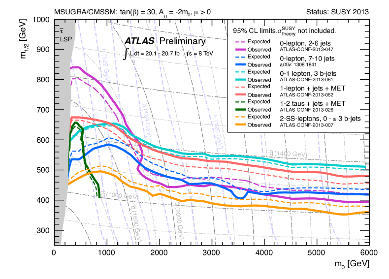
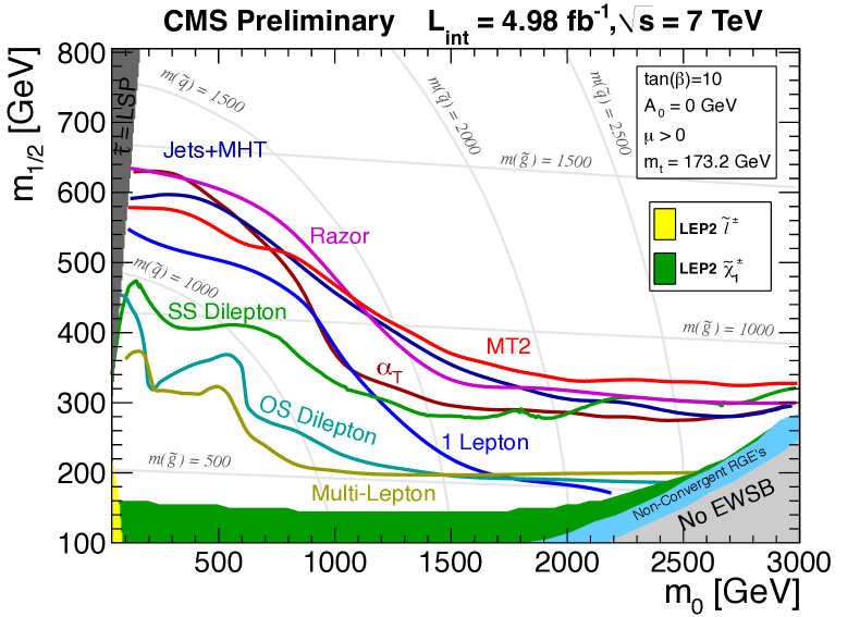
Figure 5.1: Exclusion plots at the 95% CL in the $m_{0}-m_{1/2}$ plane for CMSSM/MSUGRA for Atlas using the 8 TeV data, with $\tan\beta=30$, $A_{0}=-2m_{0}$ and $\mu>0$ (top) and for CMS using the 7 TeV data, with $\tan\beta=10$, $A_{0}=0$ and $\mu>0$ (bottom). Figures taken from [47, 48]

5.2.1.1 Specific CMSSM points

The selected scenarios in specific constrained SUSY scenarios, CMSSM and NUHM, with input parameters $m_{0}$, $m_{1/2}$, $A_{0}$, $\tan\beta$, sign($\mu$), $\delta_{1,2}$, are summarized in table 5.1 , and supplemented with $\delta^{XY}_{ij}$ as described above. Regarding CMSSM, we have chosen six SPS benchmark points [241], SPS1a, SPS1b, SPS2, SPS3, SPS4, and SPS5 and one more point with very heavy spectra (VHeavyS). Regarding NUHM, we have chosen a point with heavy SUSY spectra and light Higgs sector (HeavySLightH) and a point (BFP) that was proven in the moment of the study [242] to give the best fit to the set of low energy observables. For later reference, needed in our posterior analysis of the Higgs mass corrections, we also include in the table the corresponding MSSM Higgs masses, computed with FeynHiggs [238, 239, 240, 103] and with all flavour changing deltas switched off, i.e., $\delta^{XY}_{ij}=0$. It should be noted that our studies for these points were performed before the last data of the LHC, so some of these points (the SPS ones) are already excluded by the LHC. The study will be presented here in any case to illustrate with well known examples the phenomenology of the flavour physics and the effects on the Higgs mass corrections. The SPSX points are especially relevant since they have been studied at length in the literature. However, we will also present an updated study with currently allowed points and scenarios, that will be described in the next section. Both studies will be compared to understand also the effect of the last experiments in our constraints of the $\delta^{XY}_{ij}$ parameters and in the MSSM.

Scenarios for Constrained MSSM
points	$m_{1/2}$	$m_{0}$	$A_{0}$	$\tan\beta$	$\delta_{1}$	$\delta_{2}$	$m_{h}$	$m_{H}$	$M_{A}$	$m_{H^{\pm}}$
SPS1 a	250	100	-100	10	$0$	$0$	112	394	394	402
SPS1 b	400	200	0	30	$0$	$0$	116	526	526	532
SPS2	300	1450	0	10	$0$	$0$	115	1443	1443	1445
SPS3	400	90	0	10	$0$	$0$	115	573	572	578
SPS4	300	400	0	50	$0$	$0$	114	404	404	414
SPS5	300	150	-1000	5	$0$	$0$	111	694	694	698
VHeavyS	800	800	-800	5	$0$	$0$	120	1524	1524	1526
HeavySLightH	600	600	0	5	$-1.86$	$+1.86$	114	223	219	233
BFP	530	110	-370	27	$-84.7$	$-84.7$	120	507	507	514

Table 5.1: Values of $m_{1/2}$, $m_{0}$, $A_{0}$, $\tan\beta$, $\delta_{1}$, $\delta_{2}$ and Higgs boson masses $m_{h}$, $m_{H}$, $M_{A}$ and $m_{H^{\pm}}$ for the pre-LHC CMSSM points considered in the analysis. All parameters with mass dimension are in GeV, and ${\rm sign}(\mu)>0$ for all points. For the computations of the Higgs boson masses in this table all the $\delta^{XY}_{ij}$ are set to zero.

5.2.2 Phenomenological MSSM

We will also consider in this work (in particular for Chapters 8 and 9) scenarios directly at the lower effective SUSY breaking scale, where a much larger amount of parameters are available, and then set some relations between them to reduce their number. In that case we will not consider theoretical arguments for setting the relations, but our interest will be to obtain a phenomenologically useful model. The studied models are called “phenomenological MSSM scenarios (pMSSM)” in the literature (see, for instance, [243, 244, 236]). The assumptions for these models are the following: the breaking parameters are real, the masses and trilinear couplings appearing in the breaking terms are the same for the first and second generation at the electroweak symmetry breaking scale, and all these masses and trilinear couplings are diagonal in flavour. Being this the standard definition, we will not respect this last condition, and we will introduce non-zero elements for the non-diagonal terms. But before introducing them, the pMSSM will reduce the parameters of our model to just 22:

• $\tan\beta$: the ratio of the vevs;

• $M_{A}$: the pseudoscalar Higgs mass;

• $\mu$: the Higgs–Higgsino (supersymmetric) mass parameter (with both signs);

• $M_{1},M_{2},M_{3}$: the bino, wino and gluino mass parameters;

• $m_{\tilde{Q}_{1}},m_{\tilde{U}_{1}},m_{\tilde{D}_{1}},m_{\tilde{L}_{1}},m_{\tilde{E}_{1}}$: the first (=second) generation sfermion mass parameters;

• $A_{u},A_{d},A_{e}$: the first (=second) generation diagonal trilinear couplings;

• $m_{\tilde{Q}_{3}},m_{\tilde{U}_{3}},m_{\tilde{D}_{3}},m_{\tilde{L}_{3}},m_{\tilde{E}_{3}}$: the third generation sfermion mass parameters;

• $A_{t},A_{b},A_{\tau}$: the third generation diagonal trilinear couplings.

In this pMSSM framework, we consider several possibilities for the MSSM parameters, leading to simple patterns of SUSY masses with specific relations among them and where the number of input parameters is strongly reduced. The selected scenarios lead to predictions of $M_{h}$ that are compatible with present data over a large part of the parameter space. We have also required that all our points lead to a prediction of the anomalous magnetic moment of the muon in the MSSM that can fill the present discrepancy between the Standard Model prediction and the experimental value. Specifically, we use Refs. [245] and [246] to extract the size of this discrepancy, see also Ref. [247]:

$$(g-2)_{\mu}^{\rm exp}-(g-2)_{\mu}^{\rm SM}=(30.2\pm 9.0)\times 10^{-10}.$$ (5.30)

We then require that the SUSY contributions from charginos and neutralinos in the MSSM to one-loop level, $(g-2)_{\mu}^{\rm SUSY}$ be within the interval defined by $3\sigma$ around the central value in Eq. (5.30), namely:

$$(g-2)_{\mu}^{\rm SUSY}\in(3.2\times 10^{-10},57.2\times 10^{-10})$$ (5.31)

We will consider two kind of scenarios in the pMSSM in growing order of number of parameters: simplified pMSSM scenarios with common parameters (covered in Sections 5.2.2.1 and 5.2.2.2) and specific points (covered in Section 5.2.2.3).

5.2.2.1 pMSSM-4 scenarios

To simplify the analysis of the upper bounds of the deltas, we will focus in scenarios where the mass scales that are relevant for our studied processes are all set to common mass scales.

Regarding the LFV processes, the mass scale will be generically called here $m_{\rm SUSY-EW}$. This implies setting the slepton soft masses, the gaugino soft masses, $M_{2}$ and $M_{1}$ and the $\mu$ parameter in terms of this $m_{\rm SUSY-EW}$. It should also be noted that these same mass parameters are the relevant ones for $(g-2)_{\mu}$. The remaining relevant parameter in both LFV and $(g-2)_{\mu}$ is $\tan\beta$, and the LFV analysis of Chapter 8 will be performed in the ($m_{\rm SUSY-EW}$, $\tan\beta$) plane.

Regarding the Higgs boson, we are interested in choices of the MSSM parameters that lead to a prediction of $M_{h}$ that is compatible with LHC data, so we have to set the corresponding relevant mass parameters for this observable. These are mainly the squark soft masses and trilinear soft couplings, with particular relevance of those parameters of the third generation squarks. All these squark mass scales will be set, in this framework, relative to one single mass scale, $m_{\rm SUSY-QCD}$.

Since we wish to explore a wide range in $\tan\beta$, from 5 to 60, $M_{A}$ is fixed to $1000\,\,\mathrm{GeV}$ to ensure the agreement with the present bounds in the $(\tan\beta,M_{A})$ plane from LHC searches [248]. Finally, to reduce even further the number of input parameters we will assume an approximate GUT relation among the gaugino soft masses, $M_{2}=2M_{1}\,=\,M_{3}/4$ and the $\mu$ parameter will be set equal to $M_{2}$. Regarding the trilinear couplings, they will all be set to zero except those of the stop and sbottom sectors, being relevant for $M_{h}$, and that will be simplified to $A_{t}=A_{b}$. In summary, our scenarios in this pMSSM framework are set in terms of four input parameters: $m_{\rm SUSY-EW}$, $m_{\rm SUSY-QCD}$, $M_{2}$ and $\tan\beta$. We refer to our scenarios here as “pMSSM-4”, indicating the number of free parameters. These kind of scenarios have the advantage of reducing considerably the number of input parameters respect to the MSSM and, consequently, making easier the analysis of their phenomenological implications.

For the forthcoming numerical analysis we consider the following specific pMSSM-4 mass patterns:

• $$m_{\tilde{L}} = m_{\tilde{E}}=m_{\rm SUSY-EW}$$

  $$M_{2} = m_{\rm SUSY-EW}$$

  $$m_{\tilde{Q}} = m_{\tilde{U}}=m_{\tilde{D}}=m_{\rm SUSY-QCD}$$

  $$A_{t} = 1.3\,m_{\rm SUSY-QCD}$$

  $$m_{\rm SUSY-QCD} = 2\,m_{\rm SUSY-EW}$$ (5.32)

• $$m_{\tilde{L}} = m_{\tilde{E}}=m_{\rm SUSY-EW}$$

  $$M_{2} = m_{\rm SUSY-EW}/5$$

  $$m_{\tilde{Q}} = m_{\tilde{U}}=m_{\tilde{D}}=m_{\rm SUSY-QCD}$$

  $$A_{t} = m_{\rm SUSY-QCD}$$

  $$m_{\rm SUSY-QCD} = 2\,m_{\rm SUSY-EW}$$ (5.33)

• $$m_{\tilde{L}} = m_{\tilde{E}}=m_{\rm SUSY-EW}$$

  $$M_{2} = 300\,\,{\rm GeV}$$

  $$m_{\tilde{Q}} = m_{\tilde{U}}=m_{\tilde{D}}=m_{\rm SUSY-QCD}$$

  $$A_{t} = m_{\rm SUSY-QCD}$$

  $$m_{\rm SUSY-QCD} = m_{\rm SUSY-EW}$$ (5.34)

• $$m_{\tilde{L}} = m_{\tilde{E}}=m_{\rm SUSY-EW}$$

  $$M_{2} = m_{\rm SUSY-EW}/3$$

  $$m_{\tilde{Q}} = m_{\tilde{U}}=m_{\tilde{D}}=m_{\rm SUSY-QCD}$$

  $$A_{t} = m_{\rm SUSY-QCD}$$

  $$m_{\rm SUSY-QCD} = m_{\rm SUSY-EW}$$ (5.35)

Where we have simplified the notation for the soft sfermion masses, by using $m_{\tilde{L}}$ for $m_{\tilde{L}}=m_{\tilde{L}_{1}}=m_{\tilde{L}_{2}}=m_{\tilde{L}_{3}}$, etc. In the forthcoming numerical analysis of the maximum allowed values of the deltas within these scenarios that will be done in Chapter 8, the most relevant parameters $m_{\rm SUSY-EW}\equiv m_{\rm SUSY}$ and $\tan\beta$ will be varied within the intervals:

$$500\,\,{\rm GeV}\leq m_{\rm SUSY} \leq 2500\,\,{\rm GeV}$$

$$5\leq \tan\beta \leq 60$$ (5.36)

Due to the particular mass patterns chosen above, scenario (a) will deal with approximately equally heavy sleptons and charginos/neutralinos and with doubly heavy squarks; same for scenario (b) but with 1/5 lighter charginos/neutralinos; scenario (c) with equally heavy sleptons and squarks and charginos/neutralinos close to 300 GeV and scenario (d) with 1/3 lighter charginos/neutralinos. The values of $A_{t}$ have been selected to ensure that $M_{h}\sim 125-126\,\,\mathrm{GeV}$ over large parts of the ($M_{\rm SUSY}$, $\tan\beta$) plane.

5.2.2.2 pMSSM-4 scenarios with very heavy SUSY

The results in this section have been published in [74].

A specific variation of the previous pMSSM-4 scenarios will be defined for the Chapter 9 to study the LFV Higgs decays. In this part of the work, only the slepton sector will be relevant, so only one common SUSY mass scale will be defined, called $m_{\text{SUSY}}$. This $m_{\text{SUSY}}$ will be considered very heavy, in the interval (0.5 TeV, 10 TeV). In particular for these scenarios we choose the following setting for the relevant mass parameters:

$$m_{\tilde{L}} = m_{\tilde{E}}=m_{\text{SUSY}}\,,$$ (5.37)

$$\mu = M_{2}=a\,m_{\text{SUSY}}\,,$$ (5.38)

where $a$ is a constant coefficient that we will fix in the next sections to different values, namely, $a=\frac{1}{5}$, $\frac{1}{3}$, 1. We also set an approximate GUT inspired relation for the gaugino masses:

$$M_{2}=2M_{1}=M_{3}/4\,.$$ (5.39)

And the same notation is used for the common soft masses as in the previous section. The trilinear couplings in the slepton sector have been fixed here to the generic SUSY mass scale, $A_{\mu}=A_{e}=A_{\tau}=m_{\text{SUSY}}$. We have checked that other choices with non-vanishing values for any of the couplings of the first and second generation do not alter the conclusions of the study.

Regarding the non-diagonal trilinear couplings in the slepton sector we have also assumed a rather simple but realistic setting by relating them with the single soft SUSY-breaking mass scale, $m_{\text{SUSY}}$. Specifically, we assume the following linear relation:

$${\cal A}^{l}_{23} = {\tilde{\delta}}^{LR}_{23}m_{\text{SUSY}}\,,\,\,\,\,\,{\cal A}^{l}_{32}={\tilde{\delta}}^{LR}_{32}m_{\text{SUSY}}\,,$$ (5.40)

where the new dimensionless parameters ${\tilde{\delta}}^{LR}_{23}$ and ${\tilde{\delta}}^{LR}_{32}$ are trivially related to the previously introduced ones ${\delta}^{LR}_{23}$ and ${\delta}^{LR}_{32}$ of Eq.(5.25) by:

$${\delta}^{LR}_{23}=\left(\frac{v_{1}}{m_{\text{SUSY}}}\right){\tilde{\delta}}^{LR}_{23}\,,\,\,\,\,\,{\delta}^{LR}_{32}=\left(\frac{v_{1}}{m_{\text{SUSY}}}\right){\tilde{\delta}}^{LR}_{32}.$$ (5.41)

It is clear from Eq.(5.41) that ${\delta}^{LR}_{23}$ and ${\delta}^{LR}_{32}$ scale with $m_{\text{SUSY}}$ as $\sim\frac{1}{m_{\text{SUSY}}}$. Therefore, in the forthcoming analysis of the LFV observables, whenever the decoupling behaviour of these observables with large $m_{\text{SUSY}}$ be explored we will use instead the more suited parameters ${\tilde{\delta}}^{LR}_{23}$ and ${\tilde{\delta}}^{LR}_{32}$, which can be kept fixed to a constant value while taking large $m_{\text{SUSY}}$ values.

Concerning the size of the flavour violating trilinear couplings that are of relevance here, ${\cal A}^{l}_{23}$ and ${\cal A}^{l}_{32}$, there are well-known theoretical upper bounds that arise from vacuum stability. If any of these trilinear couplings is too large, the MSSM scalar potential develops a charge and/or colour breaking (CCB) minimum deeper than the Standard-Model-like (SML) local minimum or an unbounded from below (UFB) direction in the field space [249]. Then the requirement of the absence of these dangerous CCB minima or UFB directions implies specific upper bounds on the size of the non-diagonal trilinear couplings, and consequently on the size of the flavour changing deltas. For the case of interest here the upper bound from stability can be written simply as [249]:

$$|{\cal A}^{l}_{23}|\leq y_{\tau}\sqrt{m_{\tilde{L}_{2}}^{2}+m_{\tilde{E}_{3}}^{2}+m_{1}^{2}},$$ (5.42)

and similarly for ${\cal A}^{l}_{32}$. Here,

$$y_{\tau}=\frac{gm_{\tau}}{\sqrt{2}M_{W}\cos\beta}$$ (5.43)

is the Yukawa coupling of the tau lepton, and the squared soft mass $m_{1}^{2}$ can be written as:

$$m_{1}^{2}=(m^{2}_{A}+M_{W}^{2}+M_{Z}^{2}\sin^{2}\theta_{W})\sin^{2}\beta-\frac{1}{2}M_{Z}^{2}.$$ (5.44)

In our simplified scenarios here for the slepton, gaugino and Higgs sectors, with just three MSSM input parameters, $m_{\text{SUSY}}$, $\tan\beta$, and $m_{A}$, and by considering Eqs.(5.40) and (5.41), the previous bound implies in turn the following bound on ${\delta}^{LR}_{23}$, and correspondingly on ${\tilde{\delta}}^{LR}_{23}$ (and similar bounds for $2\leftrightarrow 3$):

$$|{\delta}^{LR}_{23}|\leq\frac{m_{\tau}}{m_{\text{SUSY}}}\sqrt{2+\frac{m_{1}^{2}}{m^{2}_{\text{SUSY}}}}\,\,,\,\,\,|{\tilde{\delta}}^{LR}_{23}|\leq y_{\tau}\sqrt{2+\frac{m_{1}^{2}}{m^{2}_{\text{SUSY}}}}.$$ (5.45)

For example, if we take $m_{\text{SUSY}}=m_{A}=1$ TeV we get upper bounds for $|{\tilde{\delta}}^{LR}_{23}|$ of ${\cal O}(0.1)$ in the low $\tan\beta$ region close to 5, and of ${\cal O}(1)$ in the large $\tan\beta$ region close to 50. These correspond to an upper bound on $|{\delta}^{LR}_{23}|$ of $\sim 0.0035$ that is nearly independent on $\tan\beta$ and it gets weaker for larger $m_{\text{SUSY}}$ values due to the scaling factor ($\frac{m_{\tau}}{m_{\text{SUSY}}}$) in Eq.(5.45).

However, the reliability of these bounds have been questioned in the literature because of the fact that the existence of deeper minima than the SML local minimum does not necessarily imply a problem whenever the lifetime of this false SML vacuum is sufficiently long. In this later case, other theoretical upper bounds based on metastability then apply. Indeed, by demanding that the lifetime of the whole observable universe staying at the SML vacuum be longer than the age of the universe the constraints on the flavour changing deltas get much more relaxed [250]. According to [250] the upper bounds on ${\delta}^{LR}_{23}$ from metastability, in contrast to the limits from stability, turn out to be independent on the Yukawa coupling, they do not decouple for asymptotically large ${m_{\text{SUSY}}}$ and they are dependent on $\tan\beta$. For instance, for $\tan\beta=3$ and ${m_{\text{SUSY}}}=5$ TeV the metastability limit on ${\delta}^{LR}_{23}$ gets weaker than its stability bound by a factor of 40, whereas for $\tan\beta=30$ and ${m_{\text{SUSY}}}=5$ TeV it is weaker by a smaller factor of 4, leading to approximate upper bounds of $|{\delta}^{LR}_{23}|\leq 0.02$ and $|{\delta}^{LR}_{23}|\leq 0.002$ respectively. This translates into an upper bound of about $|{\tilde{\delta}}^{LR}_{23}|\leq 2-3$ for $3\leq\tan\beta\leq 30$ and ${m_{\text{SUSY}}}\leq 10$ TeV. The numerical estimates of these metastability bounds are done considering each delta separately (i.e setting the other deltas to zero value) and for a specific assumption of the relevant Euclidean action providing the decay probability via tunnelling of the metastable vacuum into the global minimum. Changing the input value for the Euclidean action can increase notably the maximum allowed value up to almost doubling it, leading to roughly $|{\tilde{\delta}}^{LR}_{23}|\leq 4-6$. The effects on these bounds from switching on more than one delta at the same time have not been considered yet in the literature but they could relevantly modify these bounds. For the present work, and given the uncertainty in all these estimates of the upper bounds from stability and metastability arguments, we will consider a rather generous interval when performing the numerical estimates of branching ratios and event rates. Concretely we will choose several examples for ${\tilde{\delta}}^{LR}_{23}$ of very different size that will be taken within the wide interval $|{\tilde{\delta}}^{LR}_{23}|\leq 10$. This corresponds to $|{\delta}^{LR}_{23}|\leq 0.009$ for the particular values of $m_{\text{SUSY}}=$ 5 TeV and $\tan\beta=$ 40.

On the other hand, the values of the soft masses of the squark sector are irrelevant for LFV processes, except in the present case of LFV MSSM Higgs bosons decays that will be studied in Chapter 9 where these parameters enter in the prediction of the radiatively corrected Higgs boson masses. Since we want to identify the discovered boson with the lightest MSSM Higgs boson, we will set these parameters to values which give a prediction of $m_{h}$ compatible with the LHC data. Specifically, in Chapter 9, we fix them to the particular values $m_{\tilde{Q}}=$ $m_{\tilde{U}}=$ $m_{\tilde{D}}=$ $A_{t}=$ $A_{b}=$ 5 TeV, which we have checked provide a value for $m_{h}$ that lies within the LHC-favoured range [121 GeV, 127 GeV] for all the MSSM parameter space considered here.

In summary, the input parameters of our pMSSM-4 scenarios with very heavy SUSY are: the mass of the pseudoscalar Higgs boson, $m_{A}$, the ratio of the two Higgs vacuum expectation values, $\tan\beta$, the generic SUSY mass scale, $m_{\text{SUSY}}$, the value of $a$, and the four relevant delta parameters for the particular studied LFV Higgs decays into $\tau\mu$, $\delta_{23}^{LL}$, $\delta_{23}^{RR}$, $\delta_{23}^{LR}$ and $\delta_{23}^{RL}$ (or ${\tilde{\delta}}^{LR}_{23}$ and ${\tilde{\delta}}^{RL}_{23}$ alternatively to the two latter), which we vary within the following intervals:

• 200 GeV $\leq m_{A}\leq$ 1000 GeV,

• 1 $\leq\tan\beta\leq$ 60,

• 0.5 TeV $\leq m_{\text{SUSY}}\leq$ 10 TeV,

• $-1\leq$ $\delta_{23}^{LL}$, $\delta_{23}^{RR}$ $\leq 1$,

• $-10\leq$ ${\tilde{\delta}}_{23}^{LR}$, ${\tilde{\delta}}_{23}^{RL}$ $\leq 10$,
  (or, equivalently, $|{\delta}^{LR}_{23}|,|{\delta}^{RL}_{23}|\leq 0.009$ for $m_{\text{SUSY}}=$ 5 TeV and $\tan\beta=$ 40).

5.2.2.3 Specific pMSSM points

In this framework, we have selected six specific points in the MSSM parameter space, S1,…,S6, as examples of points that are allowed by present data, including recent LHC searches and the measurements of the muon anomalous magnetic moment. In Tab. 5.2 the values of the various MSSM parameters as well as the values of the predicted MSSM mass spectra are summarized. They were evaluated with the program FeynHiggs [238, 239, 240, 103]. For simplicity, and to reduce the number of independent MSSM input parameters in these specific pMSSM points we have assumed equal soft masses for the sleptons of the first and second generations (similarly for the squarks), equal soft masses for the left and right slepton sectors (similarly for the squarks, where $\tilde{Q}$ denotes the the “left-handed” squark sector, whereas $\tilde{U}$ and $\tilde{D}$ denote the up- and down-type parts of the “right-handed” squark sector) and also equal trilinear couplings for the stop, $A_{t}$, and sbottom squarks, $A_{b}$. In the slepton sector we just consider the stau trilinear coupling, $A_{\tau}$. The other trilinear sfermion couplings are set to zero. Regarding the soft SUSY-breaking parameters for the gaugino masses, $M_{i}$ ($i=1,2,3$), we assume again an approximate GUT inspired relation. The pseudoscalar Higgs mass $M_{A}$, and the $\mu$ parameter are also taken as independent input parameters. In summary, the six points S1,…,S6 are defined in terms of the following subset of ten input MSSM parameters:

$$m_{\tilde{L}_{1}} = m_{\tilde{L}_{2}}\;;\;m_{\tilde{L}_{3}}\;(\mbox{with~{}}m_{\tilde{L}_{i}}=m_{\tilde{E}_{i}}\,\,,\,\,i=1,2,3)$$

$$m_{\tilde{Q}_{1}} = m_{\tilde{Q}_{2}}\;;\;m_{\tilde{Q}_{3}}\;(\mbox{with~{}}m_{\tilde{Q}_{i}}=m_{\tilde{U}_{i}}=m_{\tilde{D}_{i}}\,\,,\,\,i=1,2,3)$$

$$A_{t} = A_{b}\,\,;\,\,A_{\tau}$$

$$M_{2} = 2M_{1}\,=\,M_{3}/4\,\,;\,\,\mu$$

$$M_{A} \,\,;\,\, \tan\beta$$ (5.46)

Scenarios for Phenomenological MSSM
	S1	S2	S3	S4	S5	S6
$m_{\tilde{L}_{1,2}}$	500	750	1000	800	500	1500
$m_{\tilde{L}_{3}}$	500	750	1000	500	500	1500
$M_{2}$	500	500	500	500	750	300
$A_{\tau}$	500	750	1000	500	0	1500
$\mu$	400	400	400	400	800	300
$\tan\beta$	20	30	50	40	10	40
$M_{A}$	500	1000	1000	1000	1000	1500
$m_{\tilde{Q}_{1,2}}$	2000	2000	2000	2000	2500	1500
$m_{\tilde{Q}_{3}}$	2000	2000	2000	500	2500	1500
$A_{t}$	2300	2300	2300	1000	2500	1500
$m_{\tilde{l}_{1}}-m_{\tilde{l}_{6}}$	489-515	738-765	984-1018	474-802	488-516	1494-1507
$m_{\tilde{\nu}_{1}}-m_{\tilde{\nu}_{3}}$	496	747	998	496-797	496	1499
$m_{{\tilde{\chi}}_{1}^{\pm}}-m_{{\tilde{\chi}}_{2}^{\pm}}$	375-531	376-530	377-530	377-530	710-844	247-363
$m_{{\tilde{\chi}}_{1}^{0}}-m_{{\tilde{\chi}}_{4}^{0}}$	244-531	245-531	245-530	245-530	373-844	145-363
$M_{h}$	126.6	127.0	127.3	123.1	123.8	125.1
$M_{H}$	500	1000	999	1001	1000	1499
$M_{A}$	500	1000	1000	1000	1000	1500
$M_{H^{\pm}}$	507	1003	1003	1005	1003	1502
$m_{\tilde{u}_{1}}-m_{\tilde{u}_{6}}$	1909-2100	1909-2100	1908-2100	336-2000	2423-2585	1423-1589
$m_{\tilde{d}_{1}}-m_{\tilde{d}_{6}}$	1997-2004	1994-2007	1990-2011	474-2001	2498-2503	1492-1509
$m_{\tilde{g}}$	2000	2000	2000	2000	3000	1200

Table 5.2: Selected points in the pMSSM parameter space (upper part) and their corresponding spectra for $\delta^{XY}_{ij}=0$ (lower part). All mass parameters and trilinear couplings are given in GeV.

The specific values of these ten MSSM parameters in Tab. 5.2, to be used in the forthcoming analysis of flavour violation, are chosen to provide different patterns in the various sparticle masses, but all leading to rather heavy spectra, thus they are naturally in agreement with the absence of SUSY signals at LHC. In particular all points lead to rather heavy squarks and gluinos above $1200\,\,\mathrm{GeV}$ and heavy sleptons above $500\,\,\mathrm{GeV}$ (where the LHC limits would also permit substantially lighter scalar leptons). The values of $M_{A}$ within the interval $(500,1500)\,\,\mathrm{GeV}$, $\tan\beta$ within the interval $(10,50)$ and a large $A_{t}$ within $(1000,2500)\,\,\mathrm{GeV}$ are fixed such that a light Higgs boson $h^{0}$ within the LHC-favoured range $(123,127)\,\,\mathrm{GeV}$ is obtained. It should also be noted that the large chosen values of $M_{A}\geq 500$ GeV place the Higgs sector of these specific points in the so called decoupling regime[251], where the couplings of $h^{0}$ to gauge bosons and fermions are close to the SM Higgs couplings, and the heavy $H^{0}$ couples like the pseudoscalar $A^{0}$, and all heavy Higgs bosons are close in mass. Increasing $M_{A}$ the heavy Higgs bosons tend to decouple from low energy physics and the light $h^{0}$ behaves like $H_{\rm SM}$. This type of MSSM Higgs sector seems to be in good agreement with recent LHC data[252, 17, 248]. We have checked with the code HiggsBounds [253] that the Higgs sector is in agreement with the LHC searches (where S3 is right “at the border”). Particularly, the so far absence of gluinos at LHC, forbids too low $M_{3}$ and, therefore, given the assumed GUT relation, forbids also a too low $M_{2}$. Consequently, the values of $M_{2}$ and $\mu$ are fixed as to get gaugino masses compatible with present LHC bounds.

As in the previous framework, the scenarios selected here lead to predictions of $(g-2)_{\mu}$ and $M_{h}$ that are compatible with present data over a large part of the parameter space.

Our estimate of $(g-2)_{\mu}^{\rm SUSY}$ for the six S1,…,S6 points with the code SPHENO [237] is (where FeynHiggs gives similar results), respectively,

$$(15.5\,(\mbox{S1}),\,13.8\,(\mbox{S2}),\,15.1\,(\mbox{S3}),16.7\,(\mbox{S4}),\,6.1\,(\mbox{S5}),\,7.9\,(\mbox{S6}))\,\times 10^{-10}$$ (5.47)

which are clearly within the previous allowed interval. The relatively low values of $(g-2)_{\mu}^{\rm SUSY}$ are due to the relatively heavy slepton spectrum that was chosen. However, they are well within the preferred interval. These specific points will be considered in Chapters 6, 7 and 8.

5.2.3 Effects of flavour mixing in the sfermion spectrum

All the mass spectra predictions presented before are for the MFV framework where all the non-diagonal entries of the SUSY breaking terms are set to zero, namely they are valid for $\delta^{XY}_{ij}=0$. In the rest of the work we will study the effect of non-vanishing flavour mixing deltas on different observables, but before jumping into it, we will give a glimpse of the effect of flavour mixing on the sfermion masses within the proposed scenarios themselves.

As we saw in Chapter 5.1, the deltas enter in the sfermion mass and rotation matrices, and therefore they will have an effect on the sfermion spectrum and on the spectrum of all particles that get loop corrected by the sfermions. About these loop corrections, the effects in the spectrum of the Higgs sector will be studied with detail in Chapter 7. Now we can show briefly the effects on the sfermion spectrum. For this illustration we have selected here in particular the squark sector (for sleptons a similar illustration could be done). We have chosen one of the previous points, the S2 point of table 5.2, and set one by one the different $\delta^{XY}_{ij}$ parameters of the squark mass matrices (see Eqs. 5.11 to 5.16) to values between -1 and 1. The value of the six physical squark masses as we vary the deltas are shown in Figure 5.2. In the left plots are shown the stop squark masses, and in the right plots the sbottom squark masses. Only the relevant deltas for each type of masses are shown, and the results for the deltas of the changed chirality (i.e. $\delta^{RL}_{ij}$ instead of $\delta^{LR}_{ij}$) are not shown since the results are equal.

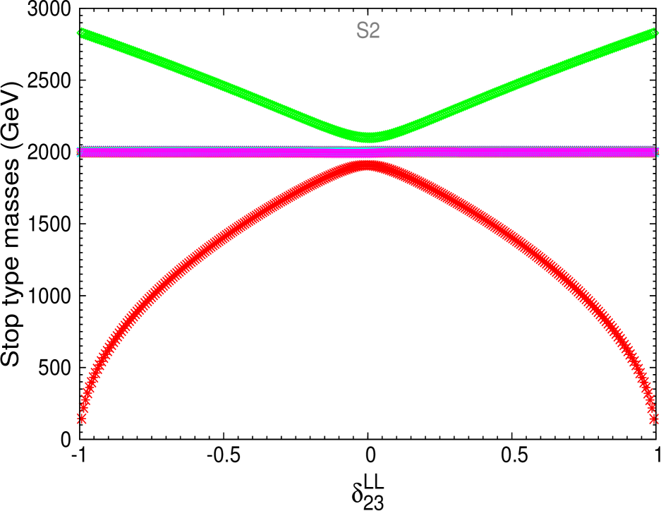
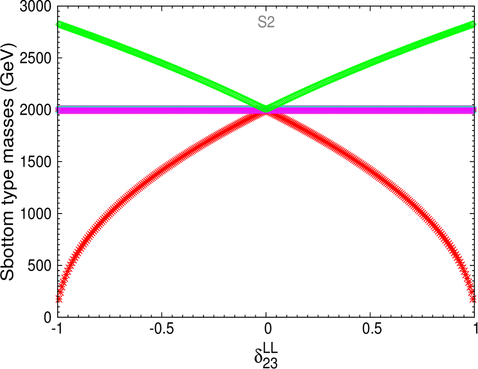
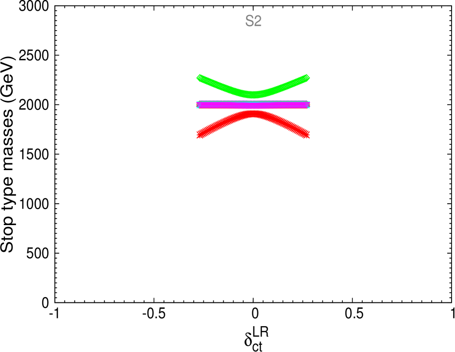
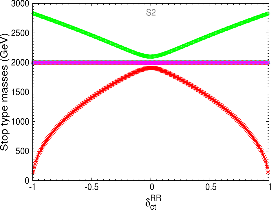
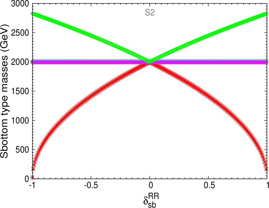
Figure 5.2: Values of the six squark masses of the top type (left column) or bottom type (right column) for the relevant NMFV deltas for each type, for the S2 point defined in 5.2.

It can be seen that most of the squarks remain almost degenerated (they are overimposed in the horizontal lines) except two, that get important positive and negative corrections from the deltas. In fact, the negative corrections can drive the value of the squark masses to values below the experimental bound around 500 GeV for the third generation (see Section 3.2.2), and thus since the sparticles have not been observed, these can set bounds for the flavour mixing parameters. However, as we will see in the next chapters, the bounds coming from $B$ physics, LFV and the Higgs masses are much more restrictive than these ones. Besides, in the middle plots of figure 5.2 we can also see that not all the values of the deltas are represented. Large values of certain deltas can generate large corrections to other particles masses, like the Higgs boson masses, and turn them negative. Obviously these leading to negative mass squared points are not shown in the plots. In particular for this S2 point, the light Higgs boson mass is the particle that will get large corrections from the deltas $\delta^{LR/RL}_{ct}$ and $\delta^{LR/RL}_{sb}$ and may turn non-physical. The size of these corrections will be studied in full detail in Section 7.3.

Chapter 6 Squark flavour mixing effects on $B$ physics

In this section we will analyze how far we can go in the flavour space in our Non-Minimal Flavour Violating SUSY scenarios. The limits on squark mixing in this chapter of it will be set by $B$-Physics observables. Since we are mainly interested in the phenomenological consequences of the flavour mixing between the third and second generations, as it was explained when it was introduced the general flavour parametrization we are using in Section 5.1.1 , we will focus on the following three B meson observables: 1) Branching ratio of the radiative $B$ decay ${\rm BR}(B\to X_{s}\gamma)$, 2) Branching ratio of the $B_{s}$ muonic decay ${\rm BR}(B_{s}\to\mu^{+}\mu^{-})$, and 3) $B_{s}-{\bar{B}_{s}}$ mass difference $\Delta M_{B_{s}}$. Another $B$ observable of interest in the present context is ${\rm BR}(B\to X_{s}l^{+}l^{-})$. However, we have not included this in our study, because the predicted rates in NMFV-SUSY scenarios for this observable are closely correlated with those from ${\rm BR}(B\to X_{s}\gamma)$ due to the dipole operators dominance in the photon-penguin diagrams mediating ${\rm BR}(B\to X_{s}l^{+}l^{-})$ decays. It implies that the restrictions on the flavour mixing $\delta^{XY}_{ij}$ parameters from ${\rm BR}(B\to X_{s}l^{+}l^{-})$ are also expected to be correlated with those from the radiative decays.

The evaluation of the observables is based on the BPHYSICS subroutine included in the SuFla code [96, 256]. For the evaluation of $\Delta M_{B_{s}}$ we have incorporated into this subroutine additional contributions from the one-loop gluino boxes [257] which are known to be very relevant in the context of NMFV scenarios [258, 259, 260].

The scenarios and points that will be worked on here were presented in Section 5.2. The summary of the relevant features for our analysis of these three B meson observables is given in the following.

The results in this chapter have been published in [71] and [75].

6.1 Implications for ${\rm BR}(B\to X_{s}\gamma)$

The relevant effective Hamiltonian for this decay is given in terms of the Wilson coefficients $C_{i}$ and operators $O_{i}$ by:

$$\mathcal{H}_{\rm eff}=-\frac{4G_{F}}{\sqrt{2}}V_{\rm CKM}^{ts*}V_{\rm CKM}^{tb}\sum_{i=1}^{8}(C_{i}O_{i}+C^{\prime}_{i}O^{\prime}_{i}).$$ (6.1)

Where the primed operators can be obtained from the unprimed ones by replacing $L\leftrightarrow R$. The complete list of operators can be found, for instance, in [261]. In the context of SUSY scenarios with the MSSM particle content and MFV, only two of these operators get relevant contributions, the so-called photonic dipole operator $O_{7}$ and gluonic dipole operator $O_{8}$ given, respectively, by:

$$O_{7}=\frac{e}{16\pi^{2}}m_{b}\left(\bar{s}_{L}\sigma^{\mu\nu}b_{R}\right)F_{\mu\nu},$$ (6.2)

$$O_{8}=\frac{g_{3}}{16\pi^{2}}m_{b}\left(\bar{s}_{L}\sigma^{\mu\nu}T^{a}b_{R}\right)G_{\mu\nu}^{a}.$$ (6.3)

We have omitted the colour indices here for brevity. Within NMFV also $O^{\prime}_{7,8}$ have to be taken into account:

$$O^{\prime}_{7}=\frac{e}{16\pi^{2}}m_{b}\left(\bar{s}_{R}\sigma^{\mu\nu}b_{L}\right)F_{\mu\nu},$$ (6.4)

$$O^{\prime}_{8}=\frac{g_{3}}{16\pi^{2}}m_{b}\left(\bar{s}_{R}\sigma^{\mu\nu}T^{a}b_{L}\right)G_{\mu\nu}^{a}.$$ (6.5)

The Wilson coefficients at the SUSY scale are obtained as usual by the matching procedure of the proper matrix element being computed from the previous effective Hamiltonian to the corresponding matrix elements being computed from the specific SUSY model, the NMFV-MSSM in our case. These Wilson coefficients encode, therefore, the contributions to ${\rm BR}(B\to X_{s}\gamma$) from the loops of the SUSY and Higgs sectors of the MSSM with NMFV. The effects from squark flavour mixings that are parametrized by the $\delta^{XY}_{ij}$, are included in this observable via the squark physical masses and rotation matrices, given in Section 5.1.1, that appear in the computation of the matrix element at the one loop level and, therefore, are also encoded in the Wilson coefficients. The explicit expressions for these coefficients in the MSSM, in terms of the particles and sparticles physical basis, can be found, for instance, in refs. [262, 263, 264]. We have included in our analysis the most relevant loop contributions to the Wilson coefficients, concretely: 1) loops with Higgs bosons, 2) loops with charginos and 3) loops with gluinos. It should be noted that, at one loop order, the gluino loops do not contribute in MFV scenarios, but they are very relevant (dominant in many cases) in the present NMFV scenarios.

Once the Wilson coefficients are known at the effective low energy SUSY scale, they are evolved with the proper Renormalization Group Equations down to the typical low-energy scale for this process. As a consequence of this running the previous operators mix and the corresponding Wilson coefficients get involved in the computation of the $B\to X_{s}\gamma$ decay rate. The RGE-running is done in two steps: The first one is from the SUSY scale down to the electroweak scale, and the second one is from this electroweak scale down to the B-physics scale. For the first step, we use the LO-RGEs for the relevant Wilson coefficients as in [264] and fix six active quark flavours in this running. For the second running we use the NLO-RGEs as in [265] and fix, correspondingly, five active quark flavours. For the charged Higgs sector we use the NLO formulas for the Wilson coefficients as in [266].

The resummation of scalar induced large $\tan\beta$ effects is performed, as usual, by the effective Lagrangian approach that parametrizes the one-loop generated effective couplings between the ${\cal H}_{2}$ Higgs doublet and the down type quarks in softly broken SUSY models [267]. A necessary condition to take into account all $\tan\beta$-enhanced terms in flavour changing amplitudes is the diagonalization of the down-type quark mass matrix in the presence of these effective couplings [99, 100, 268]. A summary of this effective Lagrangian formalism for the resummation of large $\tan\beta$ effects in the three $B$ observables of our interest, within the context of MFV scenarios, can be found in [269]. We follow here the treatment of [270] where the resummation of large $\tan\beta$ effects via effective Lagrangians is generalised to the case where the effective ${\bar{d}}^{i}_{R}d^{j}_{L}{\cal H}^{0}_{2}$ coupling contains also non-minimal sources of flavour mixing. It should be noted that the most relevant scalar induced large $\tan\beta$ effects for the present work are those generated by one-loop diagrams with gluino-sbottom and chargino-stop inside the loops. The large $\tan\beta$ resummation effects and the relevance of other chirally enhanced corrections to FCNC processes within the NMFV context have recently been studied exhaustively also in [271, 272] (previous studies can be found, for instance, in Refs. [273, 274, 275]).

The total branching ratio for this decay is finally estimated by adding the new contributions from the SUSY and Higgs sectors to the SM rate. More specifically, we use Eq.42 of [265] for the estimate of ${\rm BR}(B\to X_{s}\gamma)$ in terms of the ratios of the Wilson coefficients $C_{7,8}$ and $C^{\prime}_{7,8}$ (including all the mentioned new contributions) divided by the corresponding $C_{7,8}^{\rm SM}$ in the SM.

For the numerical estimates of ${\rm BR}(B\to X_{s}\gamma)$ we use the FORTRAN subroutine BPHYSICS (modified as to include the contributions from $C^{\prime}_{7,8}$ which were not included in its original version) included in the SuFla code, that incorporates all the above mentioned ingredients[96, 256]. Subleading NLO MSSM corrections were evaluated in [276, 277]. However, their effect on our evaluations would be minor.

6.2 Implications for ${\rm BR}(B_{s}\to\mu^{+}\mu^{-})$

The relevant effective Hamiltonian for this process is [278, 279]:

$$\mathcal{H}_{\rm eff}=-\frac{G_{F}\alpha}{\sqrt{2}\pi}V_{\rm CKM}^{ts*}V_{\rm CKM}^{tb}\sum_{i}(C_{i}O_{i}+C^{\prime}_{i}O^{\prime}_{i}),$$ (6.6)

where the operators $O_{i}$ are given by:

$${O}_{10} =\left(\bar{s}\gamma^{\nu}P_{L}b\right)\left(\bar{\mu}\gamma_{\nu}\gamma_{5}\mu\right), {O}_{10}^{\prime} =\left(\bar{s}\gamma^{\nu}P_{R}b\right)\left(\bar{\mu}\gamma_{\nu}\gamma_{5}\mu\right),$$

$${O}_{S} =m_{b}\left(\bar{s}P_{R}b\right)\left(\bar{\mu}\mu\right), {O}_{S}^{\prime} =m_{s}\left(\bar{s}P_{L}b\right)\left(\bar{\mu}\mu\right),$$

$${O}_{P} =m_{b}\left(\bar{s}P_{R}b\right)\left(\bar{\mu}\gamma_{5}\mu\right), {O}_{P}^{\prime} =m_{s}\left(\bar{s}P_{L}b\right)\left(\bar{\mu}\gamma_{5}\mu\right).$$ (6.7)

We have again omitted the colour indices here for brevity.

In this case, the RG running is straightforward since the anomalous dimensions of the above involved operators are zero, and the prediction for the decay rate is simply expressed by:

$${\rm BR}(B_{s}\to\mu^{+}\mu^{-}) =\frac{G_{F}^{2}\alpha^{2}m_{B_{s}}^{2}f_{B_{s}}^{2}\tau_{B_{s}}}{64\pi^{3}}\lvert V_{\rm CKM}^{ts*}V_{\rm CKM}^{tb}\rvert^{2}\sqrt{1-4\hat{m}_{\mu}^{2}}$$

$$\times\left[\left(1-4\hat{m}_{\mu}^{2}\right)\lvert F_{S}\rvert^{2}+\lvert F_{P}+2\hat{m}_{\mu}^{2}F_{10}\rvert^{2}\right],$$ (6.8)

where $\hat{m}_{\mu}=m_{\mu}/m_{B_{s}}$ and the $F_{i}$ are given by

$$F_{S,P} =m_{B_{s}}\left[\frac{C_{S,P}m_{b}-C_{S,P}^{\prime}m_{s}}{m_{b}+m_{s}}\right], F_{10}=C_{10}-C_{10}^{\prime}.$$

Within the SM the most relevant operator is $O_{10}$ as the Higgs mediated contributions to $O_{S,P}$ can be safely neglected. It should be noted that the contribution from $O_{10}$ to the decay rate is helicity suppressed by a factor of $\hat{m}_{\mu}^{2}$ since the $B_{s}$ meson has spin zero. In contrast, in SUSY scenarios the scalar and pseudo-scalar operators, $O_{S,P}$, can be very important. This happens particularly at large $\tan\beta\mathrel{\;{\hbox{\raise 1.50696pt\hbox{$>$}}\kern-3.8889pt\kern-3.8889pt\hbox{\lower 2.79857pt\hbox{$\sim$}}}\;}30$ where the contributions to $C_{S}$ and $C_{P}$ from neutral Higgs penguin diagrams can become large and dominate the branching ratio, because in this case the branching ratio grows with $\tan\beta$ as ${\tan}^{6}\beta$. The studies in the literature of these MSSM Higgs-penguin contributions to ${\rm BR}(B_{s}\to\mu^{+}\mu^{-})$ have focused on both MFV [280, 281, 268] and NMFV scenarios [278, 270, 275, 258]. In both cases the rates for ${\rm BR}(B_{s}\to\mu^{+}\mu^{-})$ at large $\tan\beta$ can be enhanced by a few orders of magnitude compared with the prediction in the SM, therefore providing an optimal window for SUSY signals.

In the present context of SUSY-NMFV, with no preference for large $\tan\beta$ values, there are in general three types of one-loop diagrams that contribute to the previous $C_{i}$ Wilson coefficients for this $B_{s}\to\mu^{+}\mu^{-}$ decay: 1) Box diagrams, 2) $Z$-penguin diagrams and 3) neutral Higgs boson $H$-penguin diagrams, where $H$ denotes the three neutral MSSM Higgs bosons. In our numerical estimates we have included what are known to be the dominant contributions to these three types of diagrams [278]: chargino contributions to box and Z-penguin diagrams and chargino and gluino contributions to $H$-penguin diagrams.

Regarding the resummation of large $\tan\beta$ effects we have followed the same effective Lagrangian formalism as explained in the previous case of $B\to X_{s}\gamma$. In the case of contributions from $H$-penguin diagrams to $B_{s}\to\mu^{+}\mu^{-}$ this resummation is very relevant and it has been generalised to NMFV-SUSY scenarios in [270].

For the numerical estimates we use again the BPHYSICS subroutine included in the SuFla code [96, 256] which incorporates all the ingredients that we have pointed out above.

6.3 Implications for $\Delta M_{B_{s}}$

The relevant effective Hamiltonian for $B_{s}-{\bar{B}_{s}}$ mixing and, hence, for the $B_{s}/{\bar{B}_{s}}$ mass difference $\Delta M_{B_{s}}$ is:

$$\mathcal{H}_{\rm eff}=\frac{G_{F}^{2}}{16\pi^{2}}M_{W}^{2}\left(V_{\rm CKM}^{tb*}{}V_{\rm CKM}^{ts}\right)^{2}\sum_{i}C_{i}O_{i}.$$ (6.9)

In the SM the most relevant operator is:

$$O^{VLL} =(\bar{b}^{\alpha}\gamma_{\mu}P_{L}s^{\alpha})(\bar{b}^{\beta}\gamma^{\mu}P_{L}s^{\beta}).$$ (6.10)

Where we have now written explicitly the colour indices. In scenarios beyond the SM, as the present NMFV MSSM, other operators are also relevant:

$$O^{LR}_{1} =(\bar{b}^{\alpha}\gamma_{\mu}P_{L}s^{\alpha})(\bar{b}^{\beta}\gamma^{\mu}P_{R}s^{\beta}), O^{LR}_{2} =(\bar{b}^{\alpha}P_{L}s^{\alpha})(\bar{b}^{\beta}P_{R}s^{\beta}),$$ (6.11)

$$O^{SLL}_{1} =(\bar{b}^{\alpha}P_{L}s^{\alpha})(\bar{b}^{\beta}P_{L}s^{\beta}), O^{SLL}_{2} =(\bar{b}^{\alpha}\sigma_{\mu\nu}P_{L}s^{\alpha})(\bar{b}^{\beta}\sigma^{\mu\nu}P_{L}s^{\beta}),$$ (6.12)

and the corresponding operators $O^{VRR}$ and $O^{SRR}_{i}$ that can be obtained by replacing $P_{L}\leftrightarrow P_{R}$ in (6.10) and (6.12). The mass difference $\Delta M_{B_{s}}$ is then evaluated by taking the matrix element

$$\Delta M_{B_{s}}=2\lvert\langle\bar{B}_{s}\lvert\mathcal{H}_{\rm eff}\rvert B_{s}\rangle\rvert,$$ (6.13)

where $\langle\bar{B}_{s}\lvert\mathcal{H}_{\rm eff}\rvert B_{s}\rangle$ is given by

$$\langle\bar{B}_{s}\lvert\mathcal{H}_{\rm eff}\rvert B_{s}\rangle= \frac{G_{F}^{2}}{48\pi^{2}}M_{W}^{2}m_{B_{s}}f^{2}_{B_{s}}\left(V_{\rm CKM}^{tb*}V_{\rm CKM}^{ts}\right)^{2}\sum_{i}P_{i}C_{i}\left(\mu_{W}\right).$$ (6.14)

Here $m_{B_{s}}$ is the $B_{s}$ meson mass, and $f_{B_{s}}$ is the $B_{s}$ decay constant. The coefficients $P_{i}$ contain the effects due to RG running between the electroweak scale $\mu_{W}$ and $m_{b}$ as well as the relevant hadronic matrix element. We use the coefficients $P_{i}$ from the lattice calculation [282]:

$$P^{VLL}_{1}= 0.73, P^{LR}_{1}= -1.97, P^{LR}_{2}= 2.50, P^{SLL}_{1}= -1.02, P^{SLL}_{2}= -1.97.$$ (6.15)

The coefficients $P^{VRR}_{1}$, etc., may be obtained from those above by simply exchanging $L\leftrightarrow R$.

In the present context of SUSY-NMFV, again with no preference for large $\tan\beta$ values, and besides the SM loop contributions, there are in general three types of one-loop diagrams that contribute to the previous $C_{i}$ Wilson coefficients for $B_{s}-{\bar{B}_{s}}$ mixing: 1) Box diagrams, 2) $Z$-penguin diagrams and 3) double Higgs-penguin diagrams. In our numerical estimates we have included what are known to be the dominant contributions to these three types of diagrams in scenarios with non-minimal flavour violation (for a review see, for instance, [258]): gluino contributions to box diagrams, chargino contributions to box and Z-penguin diagrams, and chargino and gluino contributions to double $H$-penguin diagrams. As in the previous observables, the total prediction for $\Delta M_{B_{s}}$ includes, of course, the SM contribution.

Regarding the resummation of large $\tan\beta$ effects we have followed again the effective Lagrangian formalism, generalised to NMFV-SUSY scenarios [270], as in the previous cases of $B\to X_{s}\gamma$ and $B_{s}\to\mu^{+}\mu^{-}$. It should be noted that, in the case of $\Delta M_{B_{s}}$, the resummation of large $\tan\beta$ effects is very relevant for the double $H$-penguin contributions, which grow very fast with $\tan\beta$.

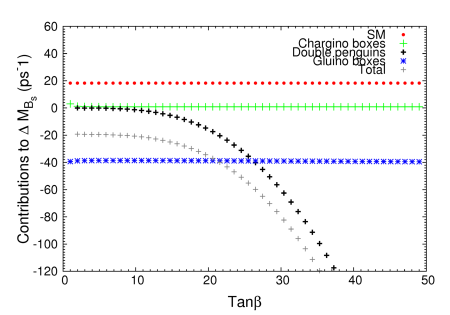
Figure 6.1: Relevant contributions to $\Delta M_{B_{s}}$ in NMFV-SUSY scenarios as a function of $\tan\beta$. They include: SM, Double Higgs penguins, gluino boxes and chargino boxes. The total prediction for $\Delta M_{B_{s}}$ should be understood here as $\Delta M_{B_{s}}=|{\rm Total}|$. The parameters are set to $\delta^{LL}_{23}=\delta^{RR}_{sb}=0.1$,$m_{\tilde{q}}=500\,\,\mathrm{GeV}$, $A_{t}=-m_{\tilde{q}}$, $m_{\tilde{g}}=\sqrt{2}m_{\tilde{q}}$, $\mu=m_{\tilde{q}}$, and $M_{A}=300\,\,\mathrm{GeV}$. The other flavour changing deltas are set to zero.

For the numerical estimates we have modified the BPHYSICS subroutine included in the SuFla code [96, 256] which incorporates all the ingredients that we have pointed out above, except the contributions from gluino boxes. These contributions are known to be very important for $B_{s}-{\bar{B}_{s}}$ mixing in SUSY scenarios with non-minimal flavour violation [259, 260, 258] and therefore they must be included into our analysis of $\Delta M_{B_{s}}$. Concretely, we have incorporated them into the BPHYSICS subroutine by adding the full one-loop formulas for the gluino boxes of [257] to the other above quoted contributions that were already included in the code. In order to illustrate the relevance of these gluino contributions in our analysis of $\Delta M_{B_{s}}$, we show in Fig.6.1 each separate contribution as a function of $\tan\beta$ in a particular example with $\delta^{LL}_{23}=\delta^{RR}_{sb}=0.1$, that we have chosen for comparison with [258]. The other flavour changing deltas are set to zero, and the other relevant MSSM parameters are set to $m_{\tilde{q}}=500\,\,\mathrm{GeV}$, $A_{t}=-m_{\tilde{q}}$, $m_{\tilde{g}}=\sqrt{2}m_{\tilde{q}}$, $\mu=m_{\tilde{q}}$, and $M_{A}=300\,\,\mathrm{GeV}$, as in Fig.24 of [258]. We clearly see in Fig.6.1 that it is just in the very large $\tan\beta$ region where double Higgs- penguins dominate. For moderate and low $\tan\beta$ values, $\tan\beta\leq 20$ (which is a relevant region for our numerical analysis, see below) the gluino boxes fully dominates the SUSY corrections to $\Delta M_{B_{s}}$ and compete with the SM contributions. Our numerical estimate in this plot is in complete agreement with the results in [258] (see, in particular, Fig.24 of this reference) which analyzed and compared in full detail these corrections.

6.4 Numerical results on constraints from $B$ observables

In the following sections we present our numerical results for the three $B$ observables in the NMFV-SUSY scenarios and a discussion on the allowed values for the flavour changing deltas, $\delta^{XY}_{ij}$.

The discussion will be structured in two different sections. The first one will be devoted to the CMSSM scenarios, defined in Section 5.2.1.1, that contains the classical SPS benchmark points that have been studied exhaustively during years before the starting of the LHC and that we choose here as illustrative examples. These points will show us how the observables behave with respect to the different parameters through a general set of scenarios. However, when the first buzz of the collisions came out of the LHC all these scenarios grew old immediately, and new scenarios were required to accommodate the new experimental situation. In the second section a set of presently allowed scenarios with heavier SUSY particles defined in 5.2.2.3 will be covered, taking into account the fact that SUSY has not appeared yet in the LHC.

In the next sections the predictions for ${\rm BR}(B\to X_{s}\gamma)$, ${\rm BR}(B_{s}\to\mu^{+}\mu^{-})$ and $\Delta M_{B_{s}}$ versus the various $\delta^{XY}_{ij}$ will be shown. For this analysis, we have assumed that just one at a time of these deltas is not vanishing. Results for two non-vanishing deltas will be shown later. The following seven flavour changing deltas are considered: $\delta^{LL}_{23}$, $\delta^{LR}_{ct}$, $\delta^{LR}_{sb}$, $\delta^{RL}_{ct}$, $\delta^{RL}_{sb}$, $\delta^{RR}_{ct}$ and $\delta^{RR}_{sb}$; and we have explored delta values within the interval $-1<\delta^{XY}_{ij}<1$. In all plots, the predictions for $\delta^{XY}_{ij}=0$ represent our estimate of the corresponding observable in the MFV case. This will allow us to compare easily the results in the two kind of scenarios, NMFV and MFV.

6.4.1 Numerical results for pre-LHC allowed scenarios and pre-LHC $B$ data

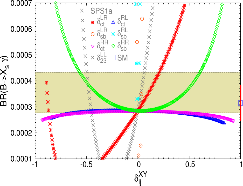
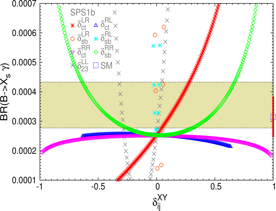
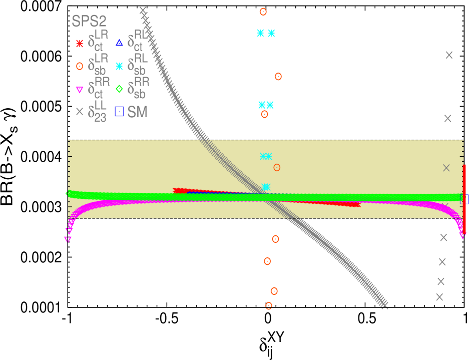
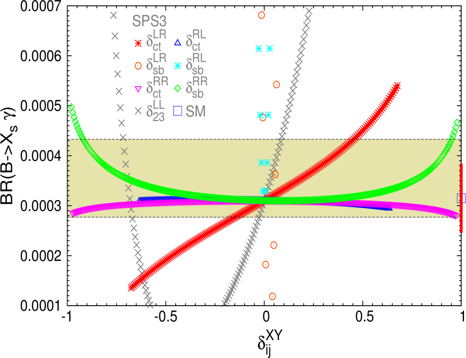
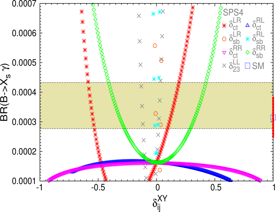
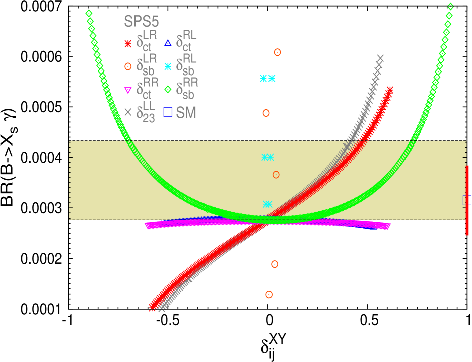
Figure 6.2: Sensitivity to the NMFV deltas in ${\rm BR}(B\to X_{s}\gamma)$ for the SPSX points of table 5.1. The experimental pre-LHC allowed $3\sigma$ area is the horizontal coloured band. The pre-LHC SM prediction and the theory uncertainty $\Delta^{\rm theo}({\rm BR}(B\to X_{s}\gamma))$ (red bar) are displayed on the right axis.

For the first study we analyze the results of the six SPS points of the CMSSM scenarios, described in Section 5.2.1.1. The predictions for ${\rm BR}(B\to X_{s}\gamma)$, ${\rm BR}(B_{s}\to\mu^{+}\mu^{-})$ and $\Delta M_{B_{s}}$ versus the various $\delta^{XY}_{ij}$, for the six selected SPS points, are displayed respectively in Figs. 6.2, 6.3 and 6.4. It should be noted that some of the predicted lines in these plots do not expand along the full interval $-1<\delta^{XY}_{ij}<1$, and they are restricted to a smaller interval. This is due to the fact, as already said in the previous chapter, that for some regions of the parameter space a too large delta value can generate very large corrections to the mass of the light Higgs boson, and even lead to a negative mass squared value. These problematic points are consequently not shown in our plots.

The experimental values and the SM predictions for the three observables at the moment we first studied them, before the LHC, were the following:

For ${\rm BR}(B\to X_{s}\gamma)$ the experimental measurement of this observable [283, 284] (where we added the various contributions to the experimental error in quadrature), and its prediction within the SM [285] were:

$${\rm BR}(B\to X_{s}\gamma)_{\rm exp}=(3.55\pm 0.26)\times 10^{-4}$$ (6.16)

$${\rm BR}(B\to X_{s}\gamma)_{\rm SM}=(3.15\pm 0.23)\times 10^{-4}$$ (6.17)

In the case of ${\rm BR}(B_{s}\to\mu^{+}\mu^{-})$ the experimental upper bound for this observable [286], and the prediction within the SM [287] were:

$${\rm BR}(B_{s}\to\mu^{+}\mu^{-})_{\rm exp}<1.1\times 10^{-8}\,\,\,\,(95\%~{}{\rm CL})$$ (6.18)

$${\rm BR}(B_{s}\to\mu^{+}\mu^{-})_{\rm SM}=(3.6\pm 0.4)\times 10^{-9}$$ (6.19)

Finally, the experimental measurement [283] of $\Delta M_{B_{s}}$ (we added again the various contributions to the experimental error in quadrature), and its prediction within the SM (using the NLO expression of [288] and the error estimate of [289]) were:

$${\Delta M_{B_{s}}}_{\rm exp} =(117.0\pm 0.8)\times 10^{-10}\,\,\mathrm{MeV}~{},$$ (6.20)

$${\Delta M_{B_{s}}}_{\rm SM} =(117.1^{+17.2}_{-16.4})\times 10^{-10}\,\,\mathrm{MeV}~{}.$$ (6.21)

We have included in the right vertical axis of the figures, for comparison, the respective SM prediction for each observable. The error bars displayed are the corresponding SM uncertainties as explained above, expanded with 3${\sigma}_{\rm SM}$ errors. The shadowed horizontal bands in the case of ${\rm BR}(B\to X_{s}\gamma)$ and $\Delta M_{B_{s}}$ are their corresponding experimental measurements in (6.16), and (6.20), expanded with 3${\sigma}_{\rm exp}$ errors. In the case of ${\rm BR}(B_{s}\to\mu^{+}\mu^{-})$ the shadowed area corresponds to the allowed region by the upper bound in (6.18).

The main conclusions extracted from these figures for the three $B$ observables are summarized as follows:

• ${\rm BR}(B\to X_{s}\gamma)$:

  • Sensitivity to the various deltas:

    We find strong sensitivity to $\delta^{LR}_{sb}$, $\delta^{RL}_{sb}$, $\delta^{LL}_{23}$, $\delta^{RR}_{sb}$ and $\delta^{LR}_{ct}$, in all the studied points, for both high and low $\tan\beta$ values. The order found from the highest to the lowest sensitivity is, generically: 1) $\delta^{LR}_{sb}$ and $\delta^{RL}_{sb}$ the largest, 2) $\delta^{LL}_{23}$ the next, 3) $\delta^{LR}_{ct}$ and $\delta^{RR}_{sb}$ the next to next, and 4) slight sensitivity to $\delta^{RR}_{ct}$ and $\delta^{RL}_{ct}$.

  • Comparing the predictions with the pre-LHC experimental data:

    If we focus on the five most relevant deltas, $\delta^{LR}_{sb}$, $\delta^{RL}_{sb}$, $\delta^{LL}_{23}$, $\delta^{RR}_{sb}$ and $\delta^{LR}_{ct}$, we see clearly that tiny deviations from zero (i.e., deviations from MFV) in these deltas, and specially in the first three, produce sizeable shifts in ${\rm BR}(B\to X_{s}\gamma)$, and in many cases take it out of the pre-LHC experimental allowed band. Therefore, it is obvious from these plots that ${\rm BR}(B\to X_{s}\gamma)$ set stringent bounds on the deltas (when varying just one delta), which were particularly tight on $\delta^{LR}_{sb}$, $\delta^{RL}_{sb}$, $\delta^{LL}_{23}$, $\delta^{RR}_{sb}$, and $\delta^{LR}_{ct}$, indeed for all the studied SPS points. There are just two exceptions, where the predicted central values of ${\rm BR}(B\to X_{s}\gamma)$ are already outside the experimental band in the MFV case (all deltas set to zero), and assuming one of these three most relevant deltas to be non-vanishing, the prediction moves inside the experimental band. This happens, for instance, in the points SPS4 and SPS1b that have the largest $\tan\beta$ values of 50 and 30 respectively. Interestingly, it means that some points of the CMSSM, particularly those with large $\tan\beta$ values, that would have been excluded in the context of MFV, could be recovered as compatible with data within NMFV-SUSY scenarios.

  • Intervals of $\delta^{XY}_{ij}$ allowed by pre-LHC data:

    In order to conclude on the pre-LHC allowed delta intervals we have assumed that our predictions of ${\rm BR}(B\to X_{s}\gamma)$ within SUSY scenarios have a somewhat larger theoretical error $\Delta^{\rm theo}({\rm BR}(B\to X_{s}\gamma))$ than the SM prediction $\Delta^{\rm theo}_{\rm SM}({\rm BR}(B\to X_{s}\gamma))$ given in (6.17). As a very conservative value we use $\Delta^{\rm theo}({\rm BR}(B\to X_{s}\gamma))=0.69\times 10^{-4}$. A given $\delta^{XY}_{ij}$ value is then considered to be allowed by data if the corresponding interval, defined by ${\rm BR}(B\to X_{s}\gamma)\pm\Delta^{\rm theo}({\rm BR}(B\to X_{s}\gamma))$, intersects with the experimental band. It corresponds to adding linearly the experimental uncertainty and the MSSM theoretical uncertainty. In total a predicted ratio in the interval

    $$2.08\times 10^{-4}<{\rm BR}(B\to X_{s}\gamma)\ <5.02\times 10^{-4},$$ (6.22)

    is regarded as allowed. Our results for these allowed intervals in this pre-LHC situation are summarized in the third column of table 6.1. In this table we see again that the less constrained parameters by ${\rm BR}(B\to X_{s}\gamma)$ were $\delta^{RL}_{ct}$, and $\delta^{RR}_{ct}$. Therefore, except for the excluded SPS4 case, these two deltas could be sizeable, $|\delta^{XY}_{ij}|$ larger than ${\cal O}(0.1)$, and compatible with ${\rm BR}(B\to X_{s}\gamma)$ data.

• ${\rm BR}(B_{s}\to\mu^{+}\mu^{-})$:

  • Sensitivity to the various deltas:

    We find significant sensitivity to the NMFV deltas in scenarios with very large $\tan\beta$, as it is the case of SPS4 and SPS1b. This sensitivity is clearly due to the Higgs-mediated contribution that, grows as $\tan^{6}\beta$. The largest sensitivity is to $\delta^{LL}_{23}$. In the case of SPS4, there is also significant sensitivity to $\delta^{LR}_{sb}$, $\delta^{RR}_{sb}$ and $\delta^{LR}_{ct}$. In the SPS1b scenario there is also found some sensitivity to $\delta^{LR}_{sb}$, $\delta^{RR}_{ct}$, $\delta^{RR}_{sb}$ and $\delta^{LR}_{ct}$.

  • Comparing the predictions with the pre-LHC experimental data:

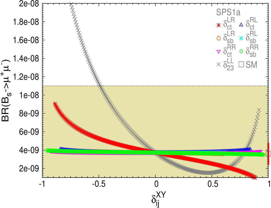
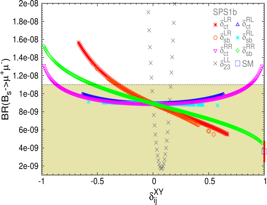
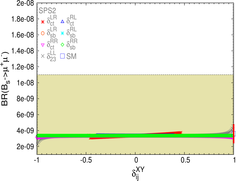
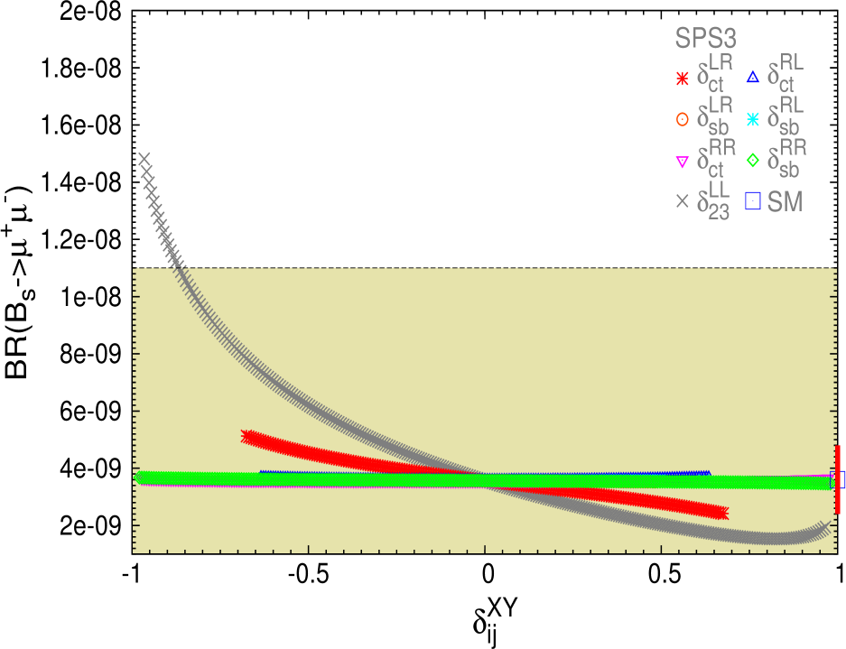
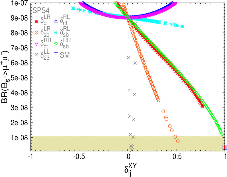
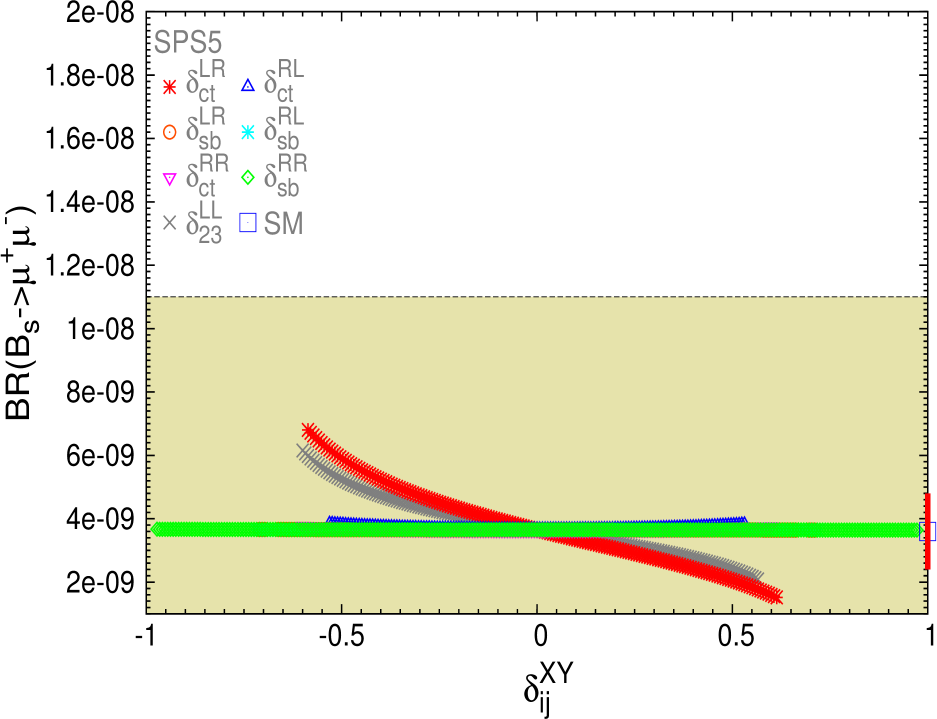
Figure 6.3: Sensitivity to the NMFV deltas in ${\rm BR}(B_{s}\to\mu^{+}\mu^{-})$ for the SPSX points of table 5.1. The experimental allowed region by the $95\%~{}{\rm CL}$ pre-LHC bound is the horizontal coloured area. The pre-LHC SM prediction and the theory uncertainty $\Delta^{\rm theo}$(${\rm BR}(B_{s}\to\mu^{+}\mu^{-})$) (red bar) are displayed on the right axis.

    Fig. 6.3 clearly shows that most of the $|\delta^{XY}_{ij}|\leq 1$ explored values were allowed by pre-LHC experimental data on ${\rm BR}(B_{s}\to\mu^{+}\mu^{-})$. It is in the points with very large $\tan\beta$, i.e SPS4 and SPS1b, where there are some relevant differences between the MFV and the NMFV predictions. First, all predictions for MFV scenarios except for SPS4, are inside the pre-LHC experimental allowed area. In the case of SPS1b, the comparison of the NMFV predictions with data constrained specially $\delta^{LL}_{23}$, but also $\delta^{LR}_{sb}$, $\delta^{RR}_{ct}$, $\delta^{RR}_{sb}$ and $\delta^{LR}_{ct}$. In the case of SPS4 some input non-vanishing values of $\delta^{LL}_{23}$, $\delta^{LR}_{sb}$ or $\delta^{RR}_{sb}$ can place the prediction inside the pre-LHC experimental allowed area. In the case of the SPS1a and SPS3 scenarios some constraints for $\delta^{LL}_{23}$ could be found.

  • Intervals of $\delta^{XY}_{ij}$ allowed by pre-LHC data:

    As in the previous observable, we assume here that our predictions for ${\rm BR}(B_{s}\to\mu^{+}\mu^{-})$ have a slightly larger error as the SM prediction in (6.19), where, however, the theory uncertainty is very small in comparison with the pre-LHC experimental bound. We choose $\Delta^{\rm theo}({\rm BR}(B_{s}\to\mu^{+}\mu^{-}))=0.12\times 10^{-8}$. Then, a given $\delta^{XY}_{ij}$ value is allowed by data if the predicted interval, defined by ${\rm BR}(B_{s}\to\mu^{+}\mu^{-})+\Delta^{\rm theo}({\rm BR}(B_{s}\to\mu^{+}\mu^{-}))$, intersects the experimental area. The upper line of the experimental area in this case is set by the $95\%~{}{\rm CL}$ upper bound given in (6.18). It implies that for a predicted ratio to be allowed it must fulfil:

    $${\rm BR}(B_{s}\to\mu^{+}\mu^{-})\ <1.22\times 10^{-8}.$$ (6.23)

    The results for the pre-LHC allowed $\delta^{XY}_{ij}$ intervals are collected in the fourth column of table 6.1. We conclude from this table that, except for scenarios with large $\tan\beta\,\geq 30$, like SPS4 and SPS1b, the size of the deltas could be sizeable, $|\delta^{XY}_{ij}|$ larger than ${\cal O}(0.1)$, and compatible with ${\rm BR}(B_{s}\to\mu^{+}\mu^{-})$ data.

• $\Delta M_{B_{s}}$:

  • Sensitivity to the various deltas:

    Generically, we find strong sensitivity to most of the NMFV deltas in all the studied points, including those with large and low $\tan\beta$ values. The pattern of the $\Delta M_{B_{s}}$ predictions as a function of the various $\delta^{XY}_{ij}$ differs substantially for each SPS point. This is mainly because in this observable there are two large competing contributions, the double Higgs penguins and the gluino boxes, with very different behaviour with $\tan\beta$, as we have seen in Fig. 6.1. In the case of SPS4 with extremely large $\tan\beta=50$, the high sensitivity to all deltas is evident in this figure. In the case of SPS5 with low $\tan\beta=5$, there is important sensitivity to all deltas, except $\delta^{RR}_{ct}$, $\delta^{LR}_{ct}$ and $\delta^{RL}_{ct}$. Generically, for all the studied points, we find the highest sensitivity to 1) $\delta^{LR}_{sb}$, $\delta^{RL}_{sb}$ and $\delta^{LL}_{23}$; 2) $\delta^{RR}_{sb}$ the next, 3) $\delta^{LR}_{ct}$ the next to next; and 4) the lowest sensitivity is to $\delta^{RL}_{ct}$ and $\delta^{RR}_{ct}$. Consequently, these last two were the less constrained ones by the pre-LHC data.

  • Comparing the predictions with the pre-LHC experimental data:

    In this case, the pre-LHC experimental allowed $3\sigma_{\rm exp}$ band is already very narrow, and all the central predictions at $\delta^{XY}_{ij}=0$, i.e. for MFV scenarios, lay indeed outside this band. However, if we assume again that our predictions suffer of a similar large uncertainty as the SM prediction, given in (6.21), then the MFV predictions are all compatible with pre-LHC data except for SPS4. It is also obvious from this figure that the predictions within NMFV, as compared to the MFV ones, lie quite generically outside the experimental allowed band, except for the above commented deltas with low sensitivity.

  • Intervals of $\delta^{XY}_{ij}$ allowed by pre-LHC data:

    We consider again, that a given $\delta^{XY}_{ij}$ value is allowed by pre-LHC $\Delta M_{B_{s}}$ data if the predicted interval $\Delta M_{B_{s}}\pm\Delta^{\rm theo}(\Delta M_{B_{s}})$, intersects the experimental band. It corresponds to adding linearly the experimental uncertainty and the theoretical uncertainty. Given the controversy on the realistic size of the theoretical error in the estimates of $\Delta^{\rm theo}(\Delta M_{B_{s}})$ in the MSSM (see, for instance, [290]), we choose a very conservative value for the theoretical error in our estimates, considerably larger than the SM value in (6.21), of $\Delta^{\rm theo}(\Delta M_{B_{s}})=51\times 10^{-10}$ MeV. This implies that a predicted mass difference in the interval

    $$63\times 10^{-10}<\Delta M_{B_{s}}\ {\rm(MeV)}<168.6\times 10^{-10},$$ (6.24)

    is regarded as allowed.

    The pre-LHC allowed intervals for the deltas that are obtained with this requirement are collected in the fifth column of table 6.1. As we have already commented, the restrictions on the b-sector parameters from $\Delta M_{B_{s}}$ were very strong, and in consequence, there were narrow intervals allowed for, $\delta^{LR}_{sb}$, $\delta^{RL}_{sb}$, and $\delta^{LL}_{23}$. In the case of $\delta^{RR}_{sb}$ there were indeed sequences of very narrow allowed intervals, which in some cases reduce to just a single allowed value. The parameters that showed a largest allowed interval, with sizeable $|\delta^{XY}_{ij}|$, larger than ${\cal O}(0.1)$, were $\delta^{RR}_{ct}$, $\delta^{RL}_{ct}$ and $\delta^{LR}_{ct}$.

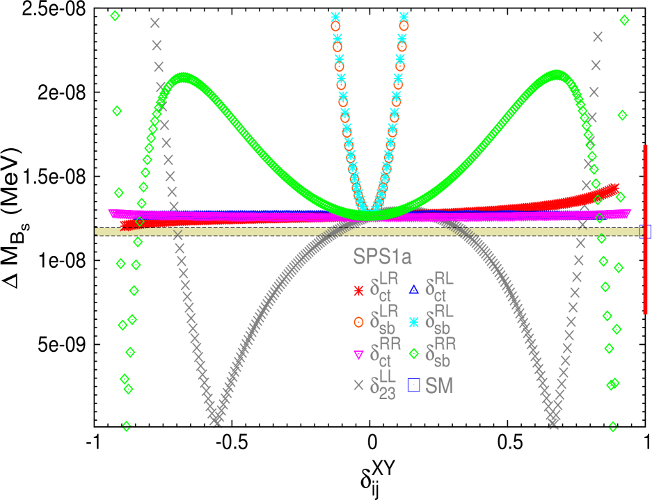
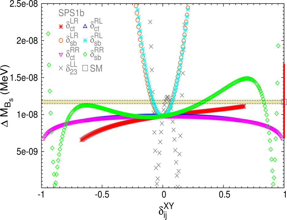
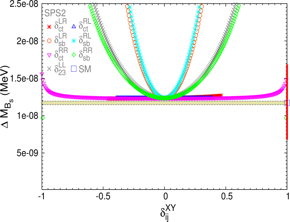
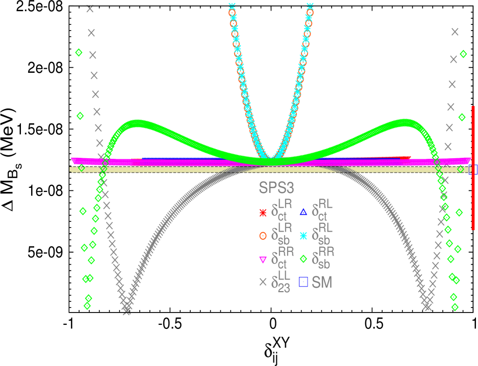
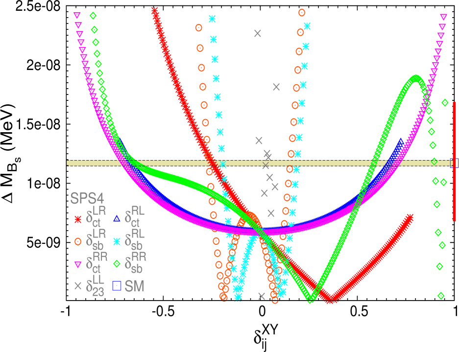
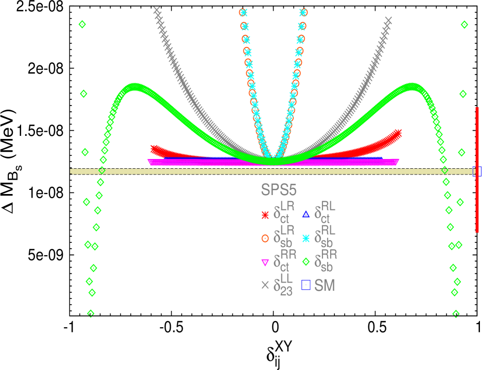
Figure 6.4: Sensitivity to the NMFV deltas in $\Delta M_{B_{s}}$ for the SPSX points of table 5.1. The experimental pre-LHC allowed $3\sigma_{\rm exp}$ area is the horizontal coloured band. The pre-LHC SM prediction and the theory uncertainty $\Delta^{\rm theo}$($\Delta M_{B_{s}}$) (red bar) are displayed on the right axis.

Total allowed pre-LHC $\delta^{XY}_{ij}$ intervals

We finally summarise in table 6.2 the total allowed intervals for all the NMFV deltas, $\delta^{XY}_{ij}$, in these pre-LHC scenarios, where we have required compatibility with the pre-LHC data of the three considered $B$ observables, ${\rm BR}(B\to X_{s}\gamma)$, ${\rm BR}(B_{s}\to\mu^{+}\mu^{-})$ and $\Delta M_{B_{s}}$. It is obvious, from the previous discussion, that the most restrictive observables were ${\rm BR}(B\to X_{s}\gamma)$ and $\Delta M_{B_{s}}$, leading to a pattern of allowed delta intervals which was clearly the intersect of their two corresponding intervals. The main conclusion from this table is that, except for SPS4 (the point SPS4 was practically excluded), the NMFV deltas in the top-sector could be sizeable $|\delta_{ct}^{XY}|$ larger than ${\cal O}(0.1)$ and still compatible with $B$ data. In particular, $\delta^{RL}_{ct}$, and $\delta^{RR}_{ct}$ were the less constrained parameters, and to a lesser extent also $\delta^{LR}_{ct}$. The parameters on the bottom-sector were, in contrast, quite constrained. The most tightly constrained were clearly $\delta^{LR}_{sb}$ and $\delta^{RL}_{sb}$, specially the first one with just some singular allowed values: either positive and of the order of $3-5\times 10^{-2}$, or negative and with a small size of the order of $-7\times 10^{-3}$; for the second the limits were around $2\times 10^{-2}$ for both positive and negative values. $\delta^{RR}_{sb}$ was the less constrained parameter in the bottom sector, with larger allowed intervals of $|\delta^{RR}_{sb}|\mathrel{\;{\hbox{\raise 1.50696pt\hbox{$<$}}\kern-3.8889pt\kern-3.8889pt\hbox{\lower 2.79857pt\hbox{$\sim$}}}\;}0.4-0.9$ depending on the scenario.

All SPS points are defined with a positive $\mu$ value. We have checked the effect of switching the sign of $\mu$. While the numerical results are changing somewhat, no qualitative change can be observed. Consequently, confining ourselves to positive $\mu$ does not constitute a general restriction of our analysis. Similar observations are made in the Higgs-sector analysis later.

The intervals allowed by $B$ data that we have presented above will be of interest for a following study in this work in the next chapter, where we will explore the size of the radiative corrections to the MSSM Higgs masses within these NMFV-MSSM scenarios and we will require compatibility with $B$ data. In the final analysis of these corrections, we will use the constraints from $B$ data as extracted from two non-vanishing deltas. As expected, these constraints vary significantly respect to the ones with just one non-vanishing delta.

		${\rm BR}(B\rightarrow X_{s}\gamma)$	${\rm BR}(B_{s}\rightarrow\mu^{+}\mu^{-})$	$\Delta M_{B_{s}}$
$\delta^{LL}_{23}$	SPS1a SPS1b SPS2 SPS3 SPS4 SPS5	(-0.51:-0.43) (-0.034:0.083) (-0.33:-0.27) (-0.014:0.062) (-0.43:0.34) (0.90:0.92) (-0.73:-0.65) (-0.083:0.12) (-0.14:-0.11) (0.0069:0.034) (-0.26:0.50)	(-0.53:0.92) (-0.014:0.16) (-0.99:0.99) (-0.90:0.97) (0.028:0.055) (-0.60:0.57)	(-0.73:-0.65) (-0.41:0.55) (0.73:0.79) (-0.090:-0.069) (-0.021:0.097) (0.14:0.17) (-0.37:0.37) (-0.86:-0.79) (-0.56:0.66) (0.83:0.89) (-0.0069)(0.021:0.055)(0.076) (-0.37:0.39)
$\delta^{LR}_{ct}$	SPS1a SPS1b SPS2 SPS3 SPS4 SPS5	(-0.89:-0.86) (-0.12:-0.097) (-0.062:0.28) (-0.083:0.36) (-0.46:0.46) (-0.43:0.61) (-0.61:-0.51) (0.041:0.23) (-0.27:0.58)	(-0.89:0.89) (-0.44:0.67) (-0.46:0.46) (-0.68:0.68) excluded (-0.59:0.61)	(-0.89:0.89) (-0.67:0.67) (-0.46:0.46) (-0.68:0.68) (-0.39:-0.021) (0.74:0.77) (-0.59:0.61)
$\delta^{LR}_{sb}$	SPS1a SPS1b SPS2 SPS3 SPS4 SPS5	(0)(0.034) (-0.0069:0) (0.048:0.055) (-0.0069:0) (0.048:0.055) (-0.0069:0) (0.048:0.055) (-0.0069)(0.034) (-0.0069:0) (0.041)	(-0.60:0.60) (-0.43:0.54) (-0.48:0.48) (-0.61:0.61) (0.49) (-0.71:0.71)	(-0.076:0.076) (-0.15:0.14) (-0.19:0.19) (-0.12:0.12) (-0.29:-0.24) (-0.10:-0.014) (0.12:0.18) (-0.090:0.090)
$\delta^{RL}_{ct}$	SPS1a SPS1b SPS2 SPS3 SPS4 SPS5	(-0.84:0.84) (-0.63:0.63) (-0.39:0.39) (-0.63:0.63) excluded (-0.53:0.53)	(-0.84:0.84) (-0.63:0.63) (-0.39:0.39) (-0.63:0.63) excluded (-0.53:0.53)	(-0.84:0.84) (-0.63:0.63) (-0.39:0.39) (-0.63:0.63) (-0.72:-0.21) (0.21:0.72) (-0.53:0.53)
$\delta^{RL}_{sb}$	SPS1a SPS1b SPS2 SPS3 SPS4 SPS5	(-0.014:0.014) (-0.021:0.021) (-0.014:0.014) (-0.021:0.021) (-0.021:-0.014)(0.014:0.021) (-0.014:0.014)	(-0.71:0.71) (-0.58:0.58) (-0.55:0.55) (-0.63:0.63) excluded (-0.72:0.72)	(-0.069:0.069) (-0.14:0.14) (-0.17:0.17) (-0.11:0.11) (-0.21:-0.17) (0.16:0.21) (-0.083:0.083)
$\delta^{RR}_{ct}$	SPS1a SPS1b SPS2 SPS3 SPS4 SPS5	(-0.93:-0.67) (-0.64:0.93) (-0.93:-0.61) (-0.56:0.90) (-1.0:0.99) (-0.97:0.97) excluded (-0.60:0.60)	(-0.93:0.93) (-0.95:0.94) (-1.0:0.99) (-0.97:0.97) excluded (-0.60:0.60)	(-0.93:0.93) (-0.98:0.98) (-1.0:0.99) (-0.98:0.97) (-0.85:-0.22) (0.22:0.85) (-0.60:0.60)
$\delta^{RR}_{sb}$	SPS1a SPS1b SPS2 SPS3 SPS4 SPS5	(-0.65:0.68) (-0.71:0.74) (-0.99:0.99) (-0.98:0.98) (-0.45:-0.18) (0.19:0.46) (-0.77:0.80)	(-0.96:0.96) (-0.73:0.98) (-0.99:0.99) (-0.98:0.98) excluded (-0.97:0.97)	(-0.91:-0.90) (-0.86:-0.80) (-0.41:0.41) (0.81:0.86) (0.90:0.91) (-0.94:-0.92) (-0.83:0.88) (0.93:0.94) (-0.99) (-0.39:0.39) (0.99) (-0.94:-0.93) (-0.88:0.88) (0.93:0.94) (-0.80:-0.028) (0.461:0.71) (0.86:0.91) (0.94:0.95) (-0.92) (-0.87:-0.78) (-0.51:0.51) (0.78:0.87) (0.92)

Table 6.1: Allowed delta intervals by ${\rm BR}(B\rightarrow X_{s}\gamma)$, ${\rm BR}(B_{s}\rightarrow\mu^{+}\mu^{-})$ and $\Delta M_{B_{s}}$ for pre-LHC allowed scenarios and pre-LHC $B$ data.

		Total allowed intervals
$\delta^{LL}_{23}$	SPS1a SPS1b SPS2 SPS3 SPS4 SPS5	(-0.034:0.083) (-0.014:0.062) (-0.37:0.34) (-0.083:0.12) (0.028:0.034) (-0.26:0.39)
$\delta^{LR}_{ct}$	SPS1a SPS1b SPS2 SPS3 SPS4 SPS5	(-0.89:-0.86) (-0.12:-0.097) (-0.062:0.28) (-0.083:0.36) (-0.46:0.46) (-0.43:0.61) excluded (-0.27:0.58)
$\delta^{LR}_{sb}$	SPS1a SPS1b SPS2 SPS3 SPS4 SPS5	(0)(0.034) (-0.0069:0) (0.048:0.055) (-0.0069:0) (0.048:0.055) (-0.0069:0) (0.048:0.055) excluded (-0.0069:0) (0.041)
$\delta^{RL}_{ct}$	SPS1a SPS1b SPS2 SPS3 SPS4 SPS5	(-0.84:0.84) (-0.63:0.63) (-0.39:0.39) (-0.63:0.63) excluded (-0.53:0.53)
$\delta^{RL}_{sb}$	SPS1a SPS1b SPS2 SPS3 SPS4 SPS5	(-0.014:0.014) (-0.021:0.021) (-0.014:0.014) (-0.021:0.021) excluded (-0.014:0.014)
$\delta^{RR}_{ct}$	SPS1a SPS1b SPS2 SPS3 SPS4 SPS5	(-0.93:-0.67) (-0.64:0.93) (-0.93:-0.61) (-0.56:0.90) (-1.0:0.99) (-0.97:0.97) excluded (-0.60:0.60)
$\delta^{RR}_{sb}$	SPS1a SPS1b SPS2 SPS3 SPS4 SPS5	(-0.41:0.41) (-0.71:0.74) (-0.99) (-0.39:0.39) (0.99) (-0.94:-0.93) (-0.88:0.88) (0.93:0.94) excluded (-0.51:0.51) (0.78:0.80)

Table 6.2: Total allowed delta intervals by ${\rm BR}(B\rightarrow X_{s}\gamma)$, ${\rm BR}(B_{s}\rightarrow\mu^{+}\mu^{-})$ and $\Delta M_{B_{s}}$ for pre-LHC allowed scenarios and pre-LHC $B$ data.

6.4.2 Numerical results for post-LHC allowed scenarios and post-LHC $B$ data

Once we have a feeling about the behaviour of the observables with respect to the different $\delta^{XY}_{ij}$, we analyze the current experimental situation. This will be done using the present bounds from $B$ physics and through a study of the set of scenarios described in Section 5.2.2.3, defined to take into account the fact that SUSY did not appear yet in the LHC, and therefore the SUSY spectra should be heavier than what was thought in its first formulations. As will be shown in the following, this heaviness of SUSY will have some impact in the considered $B$ observables when comparing with the results of the previous section.

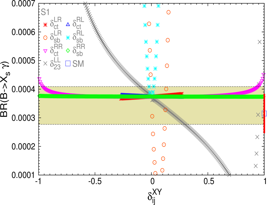
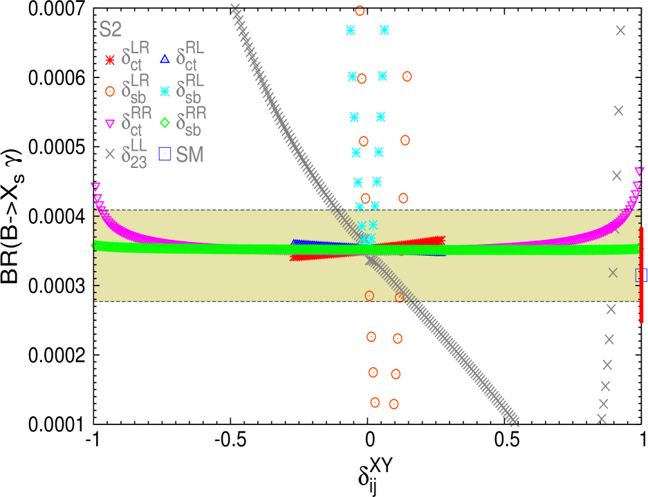
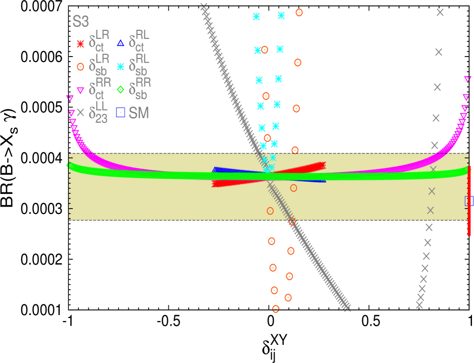
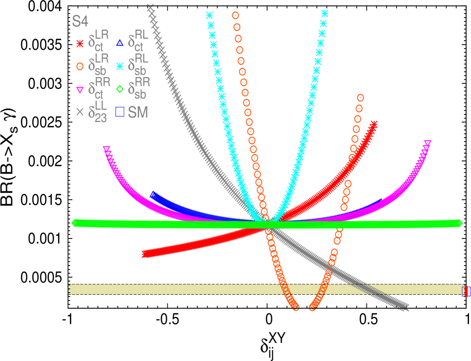
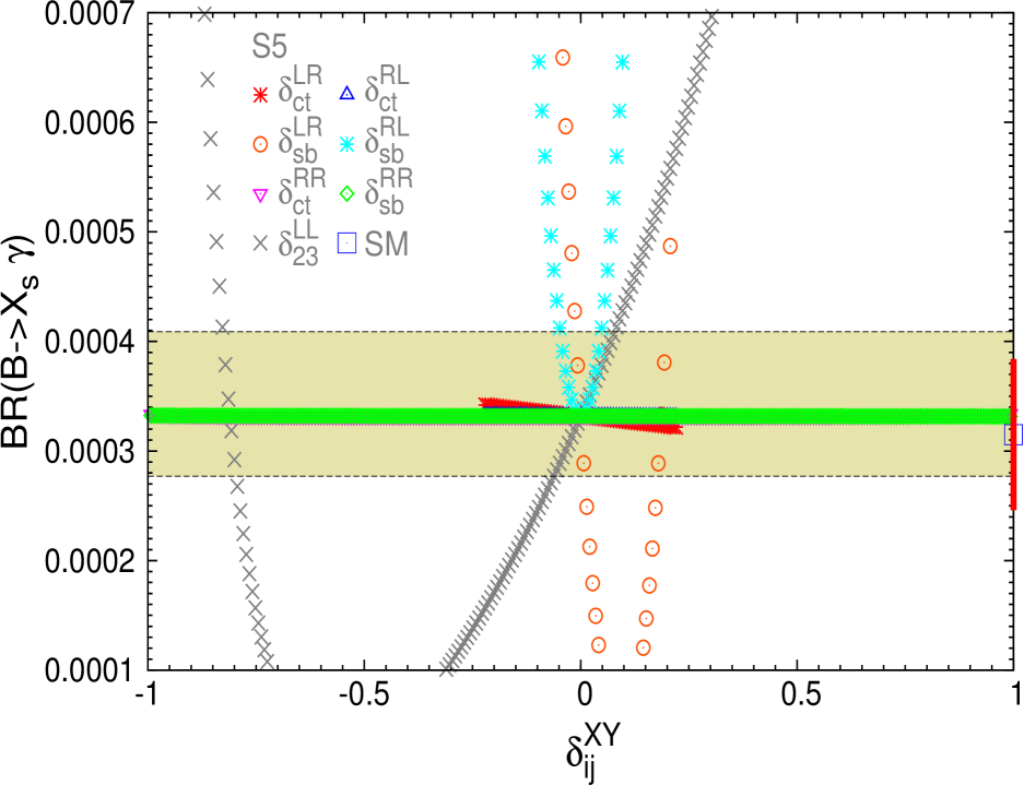
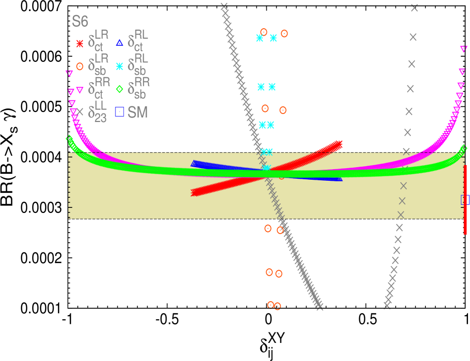
Figure 6.5: Sensitivity to the NMFV deltas in ${\rm BR}(B\to X_{s}\gamma)$ for the six post-LHC scenarios of table 5.2. The experimental allowed $3\sigma$ area is the horizontal coloured band. The SM prediction and the theory uncertainty $\Delta^{\rm theo}({\rm BR}(B\to X_{s}\gamma))$ (red bar) are displayed on the right axis.

In figures Figs. 6.5, 6.6 and 6.7 the predictions for ${\rm BR}(B\to X_{s}\gamma)$, ${\rm BR}(B_{s}\to\mu^{+}\mu^{-})$ and $\Delta M_{B_{s}}$ are shown versus the different $\delta^{XY}_{ij}$, for the six post-LHC scenarios of Section 5.2.2.3. It should be noted that again some of the predicted lines in these plots do not expand along the full interval $-1<\delta^{XY}_{ij}<1$, and they are restricted to a smaller interval. As previously, for some regions of the parameter space a too large delta value can generate very large corrections to the mass of the light Higgs boson, and its mass squared turns negative. These problematic points are consequently not included in our plots.

The present experimental values and the SM prediction for the three observables in the post-LHC period are the following:

For ${\rm BR}(B\to X_{s}\gamma)$ the experimental measurement of this observable [291] (where we have added the various contributions to the experimental error in quadrature), and its prediction within the SM [285] (that we take the same as in Eq. 6.17) are:

$${\rm BR}(B\to X_{s}\gamma)_{\rm exp}=(3.43\pm 0.22)\times 10^{-4}$$ (6.25)

$${\rm BR}(B\to X_{s}\gamma)_{\rm SM}=(3.15\pm 0.23)\times 10^{-4}$$ (6.26)

In the case of ${\rm BR}(B_{s}\to\mu^{+}\mu^{-})$ there is indeed at present an experimental measurement [292][218] instead of the previous upper bound. This measurement and the present prediction within the SM [293] are:

$${\rm BR}(B_{s}\to\mu^{+}\mu^{-})_{\rm exp}=(3.0^{+1.0}_{-0.9})\times 10^{-9}$$ (6.27)

$${\rm BR}(B_{s}\to\mu^{+}\mu^{-})_{\rm SM}=(3.23\pm 0.27)\times 10^{-9}$$ (6.28)

Finally, the experimental measurement [294] of $\Delta M_{B_{s}}$ (we have again added the various contributions to the experimental error in quadrature), and its prediction within the SM (that we take the same as in Eq. 6.21) are:

$${\Delta M_{B_{s}}}_{\rm exp} =(116.4\pm 0.5)\times 10^{-10}\,\,\mathrm{MeV}~{},$$ (6.29)

$${\Delta M_{B_{s}}}_{\rm SM} =(117.1^{+17.2}_{-16.4})\times 10^{-10}\,\,\mathrm{MeV}~{}.$$ (6.30)

We have included in the right vertical axis of the figures, for comparison, the respective SM prediction for each observable. The error bars displayed are the corresponding SM uncertainties as explained above, expanded with 3${\sigma}_{\rm SM}$ errors. The shadowed horizontal bands are the experimental measurements, expanded with 3${\sigma}_{\rm exp}$ errors.

The main conclusions extracted from these figures for the three $B$ observables are summarized as follows:

• ${\rm BR}(B\to X_{s}\gamma)$:

  • Sensitivity to the various deltas:

    We find again strong sensitivity to $\delta^{LR}_{sb}$, $\delta^{RL}_{sb}$, $\delta^{LL}_{23}$, in all the studied points, for all the studied $\tan\beta$ values. Some sensitivity to $\delta^{LR}_{ct}$ and $\delta^{RL}_{ct}$ can also be noticed. In the scenario S4 it can be found a significant sensitivity to all the deltas, except to $\delta^{RR}_{sb}$. This scenario has the lowest mass value for the squarks of the third generation and the trilinear of the top compared with the other scenarios, and large $\tan\beta$; so it is reasonable to expect a stronger general effect since it decouples less than the others and has a large $\tan\beta$ that is very relevant for these b-type observables. The order found from the highest to the lowest sensitivity is, generically: 1) $\delta^{RL}_{sb}$ and $\delta^{LR}_{sb}$ the largest, 2) $\delta^{LL}_{23}$ the next, 3) the others $\delta^{XY}_{ij}$.

    In contrast with the pre-LHC SUSY points studied in 6.4.1, now we do not find here large sensitivity with respect to $\delta^{RR}_{sb}$ and $\delta^{LR}_{ct}$. It can be seen also that all the curves are less steep than these previous ones. This is also not a surprising effect since having a heavier SUSY spectrum in these post-LHC scenarios tends to soften the effects of SUSY particles and the predicted rates are closer to the SM ones.

  • Comparing the predictions with the experimental $B$ data: The deltas with the largest impact on the observable $\delta^{LR}_{sb}$ and $\delta^{RL}_{sb}$ take us out of the experimental allowed band already with tiny values for the deltas of ${\cal O}$ (0.01). This happens also for $\delta^{LL}_{23}$, but with values that can reach the half of the area studied depending on the point. The U shape of the predicted branching ratio with some deltas make it possible for the observable to be in agreement with the experimental values for two disconnected regions. For the case of the $\delta^{LL}_{23}$ it can be seen that one of these regions lays around the maximum value considered for this $|\delta^{XY}_{ij}|$. The rest of the deltas do not get relevant constraints, except $\delta^{RR}_{ct}$ for extreme large values close to $\pm 1$.

    In the case of the point S4 whose MFV case (i.e. all deltas equal to zero) is excluded by the observable, it can be seen how non-zero values for $\delta^{LR}_{sb}$ and $\delta^{LL}_{23}$ can drive us again into the allowed area.

    The fact that some excluded MFV points of the SUSY parameter space can be allowed in the NMFV case is an important lesson for understanding the new limits of our theory.

    Comparing with the pre-LHC situation it can be seen that although the experimental band for $B$ decays became a bit narrower, the observable turned less restrictive, specially for some of the deltas whose constraints disappeared. The reason again is because in this post-LHC situation the SUSY spectrum is heavier.

  • Intervals of $\delta^{XY}_{ij}$ allowed by data:

    To conclude on the allowed delta intervals we assume that our predictions of ${\rm BR}(B\to X_{s}\gamma)$ have a somewhat larger theoretical error $\Delta^{\rm theo}({\rm BR}(B\to X_{s}\gamma))$ than the SM prediction $\Delta^{\rm theo}_{\rm SM}({\rm BR}(B\to X_{s}\gamma))$ given in (6.26). As a very conservative value we use $\Delta^{\rm theo}({\rm BR}(B\to X_{s}\gamma))=0.69\times 10^{-4}$. A given $\delta^{XY}_{ij}$ value is then considered to be allowed by data if the corresponding interval, defined by ${\rm BR}(B\to X_{s}\gamma)\pm\Delta^{\rm theo}({\rm BR}(B\to X_{s}\gamma))$, intersects with the experimental band. It corresponds to adding linearly the experimental uncertainty and the MSSM theoretical uncertainty. In total a predicted ratio in the interval

    $$2.08\times 10^{-4}<{\rm BR}(B\to X_{s}\gamma)\ <4.78\times 10^{-4},$$ (6.31)

    is now regarded as allowed. Our results for these allowed intervals are summarized in the third column of table 6.3. The less constrained parameters are $\delta^{RR}_{sb}$ and $\delta^{RR}_{ct}$ as we saw when looking at the sensitivity. These deltas can reach $|\delta^{XY}_{ij}|$ of ${\cal O}(1)$. With respect to the pre-LHC situation the constraints on $\delta^{RR}_{sb}$ have almost disappeared.

• ${\rm BR}(B_{s}\to\mu^{+}\mu^{-})$:

  • Sensitivity to the various deltas:

    We find only a relevant sensitivity to $\delta^{LL}_{23}$. Although large $\tan\beta$ scenarios were studied, that we saw in the pre-LHC scenarios enlarged the sensitivity to the deltas, the fact that we are now setting also large $M_{A}$ (because of the bounds of the recent CMS searches  [248] for MSSM neutral Higgs bosons decaying to $\tau{\bar{\tau}}$ pairs in the so-called $m_{h}^{\text{max}}$ scenario [295][296]) counteracts the enhancing effect of the large $\tan\beta$. As we commented before, this sensitivity is due to the Higgs-mediated contribution growing as $\tan^{6}\beta$ and decreasing as $M_{A}$ grows. The sensitivity to the $\delta^{LL}_{23}$ disappears in the low $\tan\beta$ scenario S5 as expected. Some sensitivity to $\delta^{RR}_{ct}$ is found in scenario S4 for large values of the delta. We recall that for some of the parameters this is the less heavy of the scenarios considered now.

  • Comparing the predictions with the experimental data:

    The experimental data changed drastically in the last time since it went from having a bound to the observable to finally getting a measurement. However, since SUSY also got more constrained, specially the presently excluded low values of $M_{A}$ for the large $\tan\beta$ case (that are the most relevant parameters here), the situation did not improve a lot respect to the pre-LHC situation. It got a bit more restrictive for some of the points in the case of $\delta^{LL}_{23}$, but now we have no constraints at all for the rest of the parameters coming from this observable.

  • Intervals of $\delta^{XY}_{ij}$ allowed by data:

    We assume here that our predictions for ${\rm BR}(B_{s}\to\mu^{+}\mu^{-})$ within SUSY scenarios have a slightly larger error as the SM prediction in (6.28). Still the theory uncertainty is very small in comparison with the experimental errors. We choose $\Delta^{\rm theo}({\rm BR}(B_{s}\to\mu^{+}\mu^{-}))=0.81\times 10^{-9}$. Then, a given $\delta^{XY}_{ij}$ value is allowed by data if the predicted interval, defined by ${\rm BR}(B_{s}\to\mu^{+}\mu^{-})\pm\Delta^{\rm theo}({\rm BR}(B_{s}\to\mu^{+}\mu^{-}))$, intersects the experimental area. To be allowed, a point should lay in the following interval:

    $${\rm BR}(B_{s}\to\mu^{+}\mu^{-})\ <6.81\times 10^{-9}.$$ (6.32)

    The results for the allowed $\delta^{XY}_{ij}$ intervals are collected in the fourth column of table 6.3. Values of $|\delta^{XY}_{ij}|$ of ${\cal O}(1)$ compatible with ${\rm BR}(B_{s}\to\mu^{+}\mu^{-})$ data can be achieved for all the deltas, except for $\delta^{LL}_{23}$ that get reduced to ${\cal O}(0.1)$.

• $\Delta M_{B_{s}}$:

  • Sensitivity to the various deltas:

    The main sensitivity is found again for $\delta^{LR}_{sb}$, $\delta^{RL}_{sb}$ and $\delta^{LL}_{23}$. Some sensitivity is found also for the $\delta^{RR}_{sb}$ parameter, specially in the S6 scenarios where it is very relevant. For the scenario S4 it can be seen a relevant sensitivity to all the deltas. In contrast, in the scenario S5 the variation of the observable with respect to all the deltas almost disappear. As we commented in the pre-LHC scenarios, different loop contributions are relevant for the observable, as shown in Fig. 6.1, depending on the value of $\tan\beta$. Comparing with these other scenarios, the general behaviour with the deltas is the same, although the general variation is a bit milder in this case.

  • Comparing the predictions with the experimental data:

    Being now smaller the variation with the deltas, one profits however from the experimental allowed band that has been reduced even more in the last time, but unfortunately the theoretical errors for the predicted points are still huge (assuming than the SUSY errors are at least as large as the SM ones). Except for the case of the S4 scenario, that lies at the border of the allowed area, for the rest of the scenarios we get constraints from this observable only for $\delta^{LL}_{23}$, and large values of $\delta^{RR}_{sb}$. Except for $\delta^{LL}_{23}$, we get softer bounds in this current allowed scenarios, as compared to the previous ones.

  • Intervals of $\delta^{XY}_{ij}$ allowed by data:

    As done previously, we consider that a given $\delta^{XY}_{ij}$ value is allowed by $\Delta M_{B_{s}}$ data if the predicted interval $\Delta M_{B_{s}}\pm\Delta^{\rm theo}(\Delta M_{B_{s}})$, intersects the experimental band. It corresponds to adding linearly the experimental uncertainty and the theoretical uncertainty. As we did before, and given the controversy on the realistic size of the theoretical error in the estimates of $\Delta^{\rm theo}(\Delta M_{B_{s}})$ in the MSSM (see, for instance, [290]), we choose a very conservative value for the theoretical error in our estimates, considerably larger than the SM value in (6.30), of $\Delta^{\rm theo}(\Delta M_{B_{s}})=51\times 10^{-10}$ MeV. This implies that a predicted mass difference in the interval

    $$63.9\times 10^{-10}<\Delta M_{B_{s}}\ {\rm(MeV)}<168.9\times 10^{-10},$$ (6.33)

    is regarded as allowed.

    The allowed intervals for the deltas are collected in the fifth column of table 6.3. The main restrictions are set to the sb-type deltas as it was expected and to $\delta^{LL}_{23}$. We observe again for some scenarios the appearance of disconnected allowed regions due to the form of the variation with respect to the deltas. Deltas of ${\cal O}(0.1)$ are allowed for all parameters, and reach up to ${\cal O}(1)$ for the $RR$ delta types.

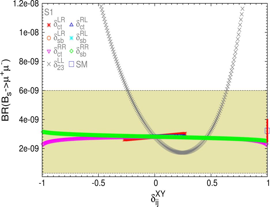
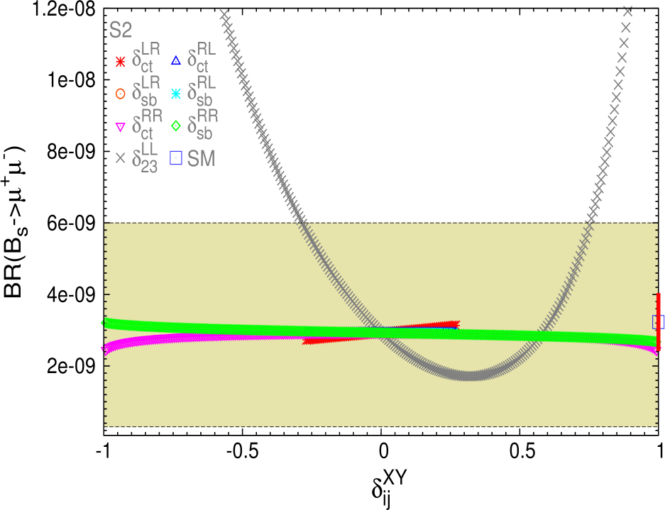
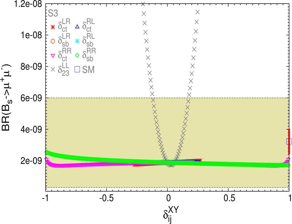
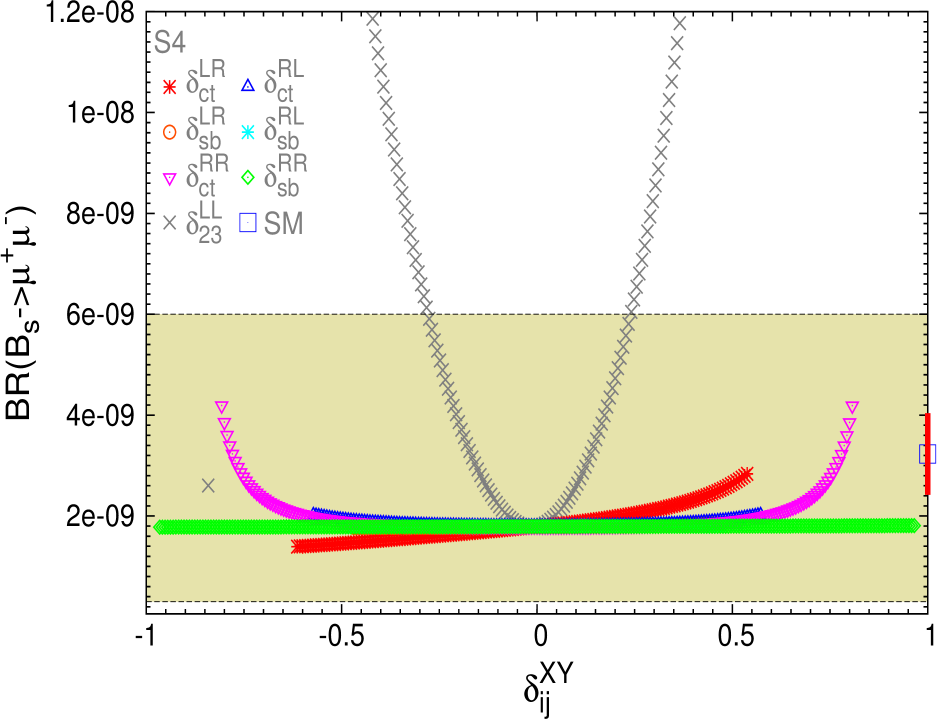
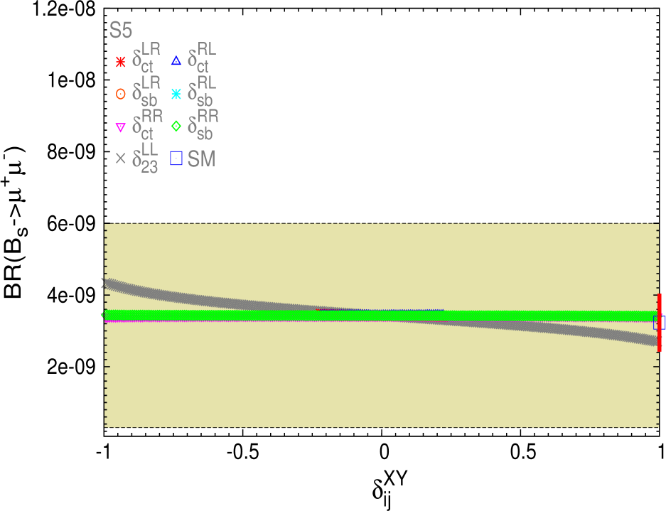
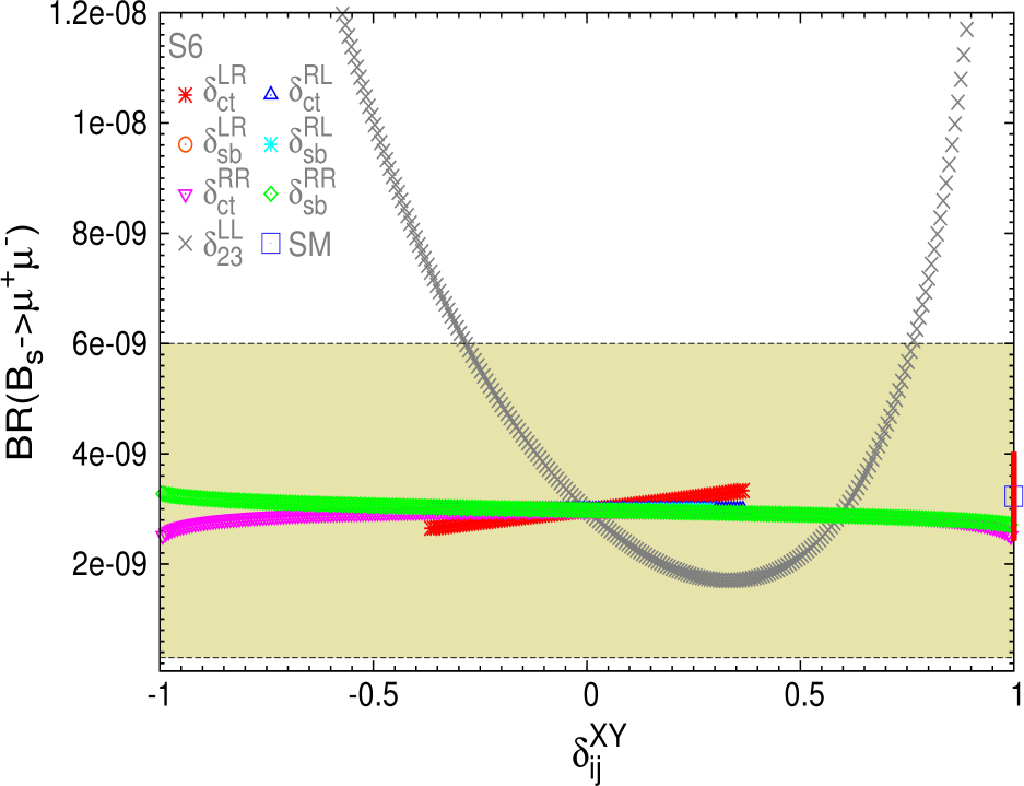
Figure 6.6: Sensitivity to the NMFV deltas in ${\rm BR}(B_{s}\to\mu^{+}\mu^{-})$ for the six post-LHC scenarios of table 5.2. The experimental allowed $3\sigma$ area is the horizontal coloured band. The SM prediction and the theory uncertainty $\Delta^{\rm theo}({\rm BR}(B_{s}\to\mu^{+}\mu^{-}))$ (red bar) are displayed on the right axis.

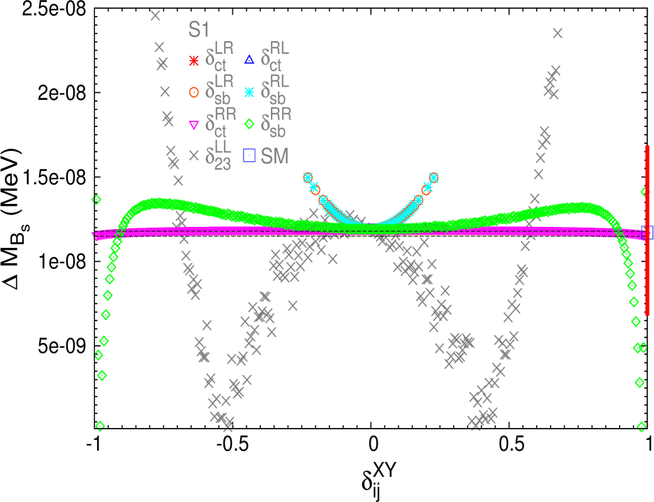
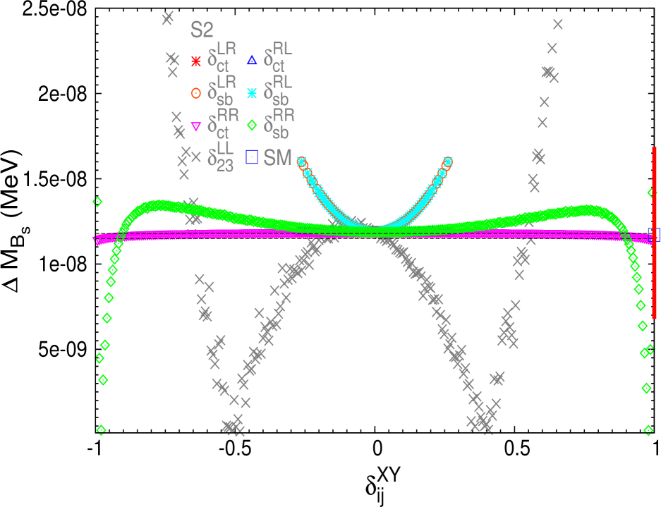
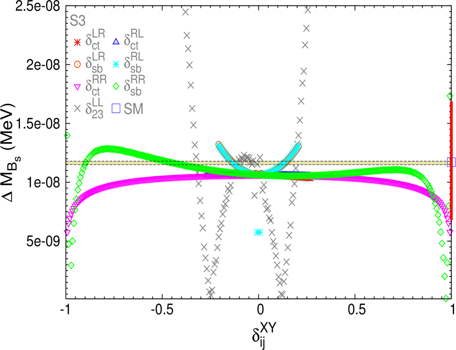
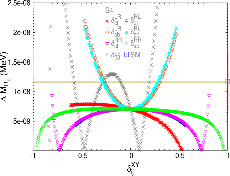
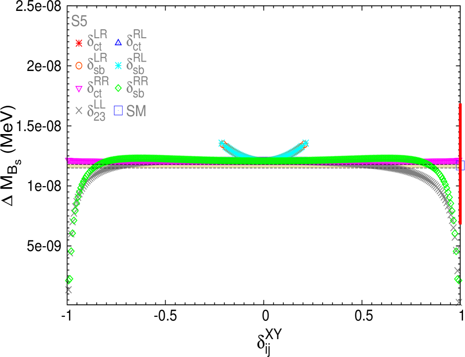
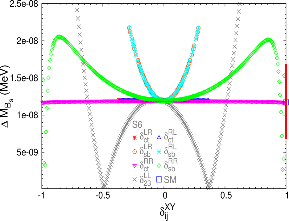
Figure 6.7: Sensitivity to the NMFV deltas in $\Delta M_{B_{s}}$ for the six post-LHC scenarios of table 5.2. The experimental allowed $3\sigma$ area is the horizontal coloured band. The SM prediction and the theory uncertainty $\Delta^{\rm theo}(\Delta M_{B_{s}})$ (red bar) are displayed on the right axis.

Total present allowed $\delta^{XY}_{ij}$ intervals and comparison with the pre-LHC situation

To conclude this section, we collect in table 6.4 the total allowed intervals for all the flavour parameters of the squark sector in the selected LHC points, being compatible with ${\rm BR}(B\to X_{s}\gamma)$, ${\rm BR}(B_{s}\to\mu^{+}\mu^{-})$ and $\Delta M_{B_{s}}$.

The main restrictions to the flavour parameters come from ${\rm BR}(B\to X_{s}\gamma)$ and in some cases from $\Delta M_{B_{s}}$ and not yet from the young measurement ${\rm BR}(B_{s}\to\mu^{+}\mu^{-})$. The most restricted deltas are $\delta^{LR}_{sb}$ and $\delta^{RL}_{sb}$ that can reach $|\delta^{XY}_{ij}|$ of ${\cal O}(0.01)$, then $\delta^{LL}_{23}$, $\delta^{LR}_{ct}$ and $\delta^{RL}_{ct}$ can be one order of magnitude larger, with the first being more restricted than the last two, and finally the less restricted are $\delta^{RR}_{ct}$ and $\delta^{RR}_{sb}$ than in general could reach a size of ${\cal O}(1)$.

We remark again the interesting fact that some of the presently excluded MFV points can be driven to the allowed area of the observables, by setting some of the deltas to a non-zero value.

It was to be expected to get larger constraints in the $sb$ sector since it is the one directly involved in the flavour changing observables we are considering. And it is also understandable that the $LR$ deltas become more restricted than the others, since they involve the trilinear couplings that are not just part of a mass term, but they enter straight in the relevant Feynman rules of the observables, and not only through the diagonalization of the mass matrices.

In general, the bounds on the squark mixing deltas are more relaxed in our scenarios S1-S6 compared to the set of benchmark scenarios that was analyzed before the LHC started operation. The scenarios investigated in the pre-LHC era contained relatively light SUSY particles, leading to relatively large corrections from NMFV effects. After the so far unsuccessful search for BSM physics at the LHC, scalar quarks masses (in particular of the first and second generation) have substantially higher lower bounds. Benchmark scenarios that take this into account (as our S1-S6) naturally permit larger values for the NMFV deltas.

As we told in advance in the last section, once we know the allowed intervals of the flavour parameters these will be explored to learn the consequences they have in the radiative corrections to the just discovered Higgs boson.

		${\rm BR}(B\rightarrow X_{s}\gamma)$	${\rm BR}(B_{s}\rightarrow\mu^{+}\mu^{-})$	$\Delta M_{B_{s}}$
$\delta^{LL}_{23}$	S1 S2 S3 S4 S5 S6	(-0.27:0.48) (0.94:0.95) (-0.23:0.32) (0.88:0.91) (-0.12:0.21) (0.79:0.83) (0.41:0.61) (-0.83:-0.78) (-0.14:0.14) (-0.076:0.14) (0.66:0.71)	(-0.28:0.66) (-0.33:0.78) (-0.13:0.19) (-0.30:0.26) (-0.99:0.99) (-0.33:0.79)	(-0.72:-0.63) (-0.41:0.28) (0.50:0.61) (-0.69:-0.59) (-0.37:0.23) (0.50:0.59) (-0.34:-0.30) (-0.19:0.06) (0.17:0.21) (-0.61:-0.54) (-0.39:0.01) (0.15:0.23) (-0.97:0.97) (-0.66:-0.57) (-0.37:0.23) (0.46:0.56)
$\delta^{LR}_{ct}$	S1 S2 S3 S4 S5 S6	(-0.27:0.27) (-0.27:0.27) (-0.27:0.27) excluded (-0.22:0.22) (-0.37:0.37)	(-0.27:0.27) (-0.27:0.27) (-0.27:0.27) (-0.61:0.54) (-0.22:0.22) (-0.37:0.37)	(-0.27:0.27) (-0.27:0.27) (-0.27:0.27) (-0.61:0.13) (-0.22:0.22) (-0.37:0.37)
$\delta^{LR}_{sb}$	S1 S2 S3 S4 S5 S6	(-0.0069:0.014) (0.12:0.13) (-0.0069:0.014) (0.11:0.13) (-0.0069:0.014) (0.11:0.13) (0.076:0.12) (0.26:0.30) (-0.014:0.021) (0.17:0.19) (0:0.0069) (0.069:0.076)	(-0.23:0.23) (-0.26:0.26) (-0.21:0.21) (-0.47:0.47) (-0.21:0.21) (-0.28:0.28)	(-0.23:0.23) (-0.26:0.26) (-0.21:0.21) (-0.39:0.42) (-0.21:0.21) (-0.20:0.20)
$\delta^{RL}_{ct}$	S1 S2 S3 S4 S5 S6	(-0.27:0.27) (-0.27:0.27) (-0.27:0.27) excluded (-0.22:0.22) (-0.37:0.37)	(-0.27:0.27) (-0.27:0.27) (-0.27:0.27) (-0.57:0.57) (-0.22:0.22) (-0.37:0.37)	(-0.27:0.27) (-0.27:0.27) (-0.27:0.27) (-0.32:0.32) (-0.22:0.22) (-0.37:0.37)
$\delta^{RL}_{sb}$	S1 S2 S3 S4 S5 S6	(-0.034:0.034) (-0.034:0.034) (-0.034:0.034) excluded (-0.062:0.062) (-0.021:0.021)	(-0.23:0.23) (-0.26:0.26) (-0.21:0.21) (-0.47:0.47) (-0.21:0.21) (-0.28:0.28)	(-0.23:0.23) (-0.26:0.26) (-0.21:0.21) (-0.40:0.40) (-0.21:0.21) (-0.20:0.20)
$\delta^{RR}_{ct}$	S1 S2 S3 S4 S5 S6	(-0.99:0.99) (-0.99:0.99) (-0.98:0.97) excluded (-0.99:0.99) (-0.96:0.94)	(-0.99:0.99) (-0.99:0.99) (-0.99:0.99) (-0.81:0.81) (-0.99:0.99) (-0.99:0.99)	(-0.99:0.99) (-0.99:0.99) (-0.99:0.99) (-0.81:-0.80) (-0.34:0.34) (0.80:0.81) (-0.99:0.99) (-0.99:0.99)
$\delta^{RR}_{sb}$	S1 S2 S3 S4 S5 S6	(-0.99:0.99) (-0.99:0.99) (-0.99:0.99) excluded (-0.99:0.99) (-0.99:0.99)	(-0.99:0.99) (-0.99:0.99) (-0.99:0.99) (-0.97:0.97) (-0.99:0.99) (-0.99:0.99)	(-0.96:0.96) (-0.96:0.96) (-0.96:0.94) (-0.70:0.54) (-0.97:0.97) (-0.97:-0.94) (-0.63:0.64) (0.93:0.97)

Table 6.3: Allowed delta intervals by ${\rm BR}(B\rightarrow X_{s}\gamma)$, ${\rm BR}(B_{s}\rightarrow\mu^{+}\mu^{-})$ and $\Delta M_{B_{s}}$ for post-LHC allowed scenarios and post-LHC $B$ data.

		Total allowed intervals
$\delta^{LL}_{23}$	S1 S2 S3 S4 S5 S6	(-0.27:0.28) (-0.23:0.23) (-0.12:0.06) (0.17:0.19) excluded (-0.83:-0.78) (-0.14:0.14) (-0.076:0.14)
$\delta^{LR}_{ct}$	S1 S2 S3 S4 S5 S6	(-0.27:0.27) (-0.27:0.27) (-0.27:0.27) excluded (-0.22:0.22) (-0.37:0.37)
$\delta^{LR}_{sb}$	S1 S2 S3 S4 S5 S6	(-0.0069:0.014) (0.12:0.13) (-0.0069:0.014) (0.11:0.13) (-0.0069:0.014) (0.11:0.13) (0.076:0.12) (0.26:0.30) (-0.014:0.021) (0.17:0.19) (0:0.0069) (0.069:0.076)
$\delta^{RL}_{ct}$	S1 S2 S3 S4 S5 S6	(-0.27:0.27) (-0.27:0.27) (-0.27:0.27) excluded (-0.22:0.22) (-0.37:0.37)
$\delta^{RL}_{sb}$	S1 S2 S3 S4 S5 S6	(-0.034:0.034) (-0.034:0.034) (-0.034:0.034) excluded (-0.062:0.062) (-0.021:0.021)
$\delta^{RR}_{ct}$	S1 S2 S3 S4 S5 S6	(-0.99:0.99) (-0.99:0.99) (-0.98:0.97) excluded (-0.99:0.99) (-0.96:0.94)
$\delta^{RR}_{sb}$	S1 S2 S3 S4 S5 S6	(-0.96:0.96) (-0.96:0.96) (-0.96:0.94) excluded (-0.97:0.97) (-0.97:-0.94) (-0.63:0.64) (0.93:0.97)

Table 6.4: Total allowed delta intervals by ${\rm BR}(B\rightarrow X_{s}\gamma)$, ${\rm BR}(B_{s}\rightarrow\mu^{+}\mu^{-})$ and $\Delta M_{B_{s}}$ for post-LHC allowed scenarios and post-LHC $B$ data.

Chapter 7 Higgs boson mass corrections from flavour mixing in the squark sector

The discovery of the Higgs boson still leaves an important question opened: what kind of Higgs boson have we discovered? Is it the new boson a signal of a new supersymmetric world or just the last undiscovered piece of our old Standard Model? The currently ongoing precision measurements on the Higgs characteristics as the mass, the couplings and the decays will be crucial to answer these questions. In this chapter we will study the Higgs boson mass corrections generated from general squark flavour mixing. We will study the size of the Higgs boson radiative mass corrections depending on the different flavour mixing $\delta^{XY}_{ij}$ parameters of the squark sector and the MSSM parameters, and we will also set constraints on the possible size of the squark flavour mixing from the present bounds on the value of the Higgs mass itself.

The results in this chapter have been published in [71] and [75].

7.1 Status and framework for the Higgs mass corrections computation

As we commented when introducing the Higgs sector in Sections 3.2.1.1 and 3.2.1.2, higher-order contributions can give large corrections to the tree-level relations (see e.g. Ref. [297] for reviews) of this sector. In the MSSM the status of higher-order corrections to the masses and mixing angles in the neutral Higgs sector is quite advanced. The full one-loop and potentially all leading two-loop corrections are known, see Ref. [240] for a review. Most recently leading three-loop corrections became available [299, 300].

However, the impact of non-minimal flavour violation in the squark sector, on the MSSM Higgs-boson masses and mixing angles, entering already at the one-loop level, has not been explored very deeply so far. A one-loop calculation taking into account the $LL$-mixing between the third and second generation of scalar up-type quarks has been performed in Ref. [254]. A full one-loop calculation of the Higgs-boson self-energies including all NMFV mixing terms had been implemented into the Fortran code FeynHiggs [238, 239, 240, 103], however no cross checks or numerical evaluations analyzing the effects of the new mixing terms were performed. Possible effects from NMFV on Higgs boson decays were investigated in [301, 303, 304, 302]. Within a similar context of NMFV there have been also studied some effects of scharm-stop flavour mixing in top-quark FCNC processes [255] and charged Higgs processes [305] as well as the implications for LHC [306, 305]. Some previous studies on the induced radiative corrections on the Higgs mass from scharm-stop flavour mixing have also been performed in [255, 306], but any effects from mixing involving the first generation of scalar quarks have been neglected. The numerical estimates in [255, 306] also neglect all the flavour mixings in the scalar down-type sector, except for those of $LL$-type that are induced from the scalar up-type sector by SU(2) invariance. In [306] they also consider one example with a particular numerical value of non-vanishing ${\tilde{s}}_{L}-{\tilde{b}}_{R}$ mixing.

We study in this chapter the consequences from NMFV in the squark sector for the MSSM Higgs-boson spectrum, where our results are obtained in full generality, i.e. all generations in the scalar up- and down-type quark sector are included in our analytical results. In the numerical analysis we focus particularly on the flavour mixing between the second and third generations. Our estimates include all type of flavour mixings, $LL$, $LR$, $RL$, and $RR$. We devote special attention to the $LR/RL$ sector. These kind of mixing effects are expected to be sizeable, since they enter the off-diagonal $A$ parameters, which appear directly in the coupling of the Higgs bosons to scalar quarks.

With respect to the scenarios, we will use the ones defined in Section 5.2. Concerning the constraints from flavour observables we take into account the most up-to-date evaluations in the NMFV MSSM for ${\rm BR}(B\to X_{s}\gamma)$, ${\rm BR}(B_{s}\to\mu^{+}\mu^{-})$ and $\Delta M_{B_{s}}$. These observables and the constraints coming from them were studied in detail in Chapter 6. Here we analyze the one-loop contributions of NMFV to the MSSM Higgs boson masses, focusing on the parameter space still allowed by the experimental flavour constraints, as it was studied in this previous chapter. In this way the full possible impact of NMFV in the MSSM on the Higgs sector can be explored. It will also be compared the situation previous to the LHC and after the LHC data.

7.2 Analytical results for the MSSM corrected Higgs boson self energies

Following the detailed prescription for the computation of the one-loop corrected Higgs boson masses given in Sections 3.2.1.1 and 3.2.1.2, one finds the analytical expressions for these masses in terms of the renormalized self-energies which, in turn, are written in terms of the unrenormalized self-energies and tadpoles. To shorten the presentation of these analytical results, it is convenient to report here just on these unrenormalized self-energies and tadpoles.

The relevant one-loop corrections have been evaluated with the help of FeynArts [307] and FormCalc [308]. For completeness the new Feynman rules included in the model file are listed in the Appendix A. All the results for the unrenormalized self-energies and tadpoles are collected in Appendix B. We have shown explicitly just the relevant contributions for the present study of the radiative corrections to the Higgs boson masses within NMFV scenarios in the squark sector, namely, the one-loop contributions from quarks and squarks. The corresponding generic Feynman-diagrams for the Higgs bosons self-energies, gauge boson self-energy diagrams and tadpole diagrams are collected in the Fig. B.1 in Appendix B. It should also be noticed that the contributions from the squarks are the only ones that differ from the usual ones of the MSSM with MFV. It should be noted also that the corrections from flavour mixing, which are the subject of our interest here, are implicit in both the $V_{\rm CKM}$, and in the values of the rotation matrices, $R^{\tilde{u}}$, $R^{\tilde{d}}$, the squark masses, $m_{\tilde{u}_{i}}$, $m_{\tilde{d}_{i}}$ ($i=1,..,6$) and the non-diagonal in flavour trilinear couplings, that appear in these formulas of the unrenormalized self-energies and tadpoles and that have been introduced in Section 5.1.1.

Finally, it is worth mentioning that we have checked the finiteness in our analytical results for the renormalized Higgs self-energies. It is obviously expected, but it is not a trivial check in the present scenarios with three generations of quarks and squarks and with flavour mixing. We have also checked that the analytical results of the self-energies in Appendix B agree with the formulas in FeynHiggs [238, 239, 240, 103]. Each one of the terms contained in the Appendix B was compared with the corresponding term in FeynHiggs. During this process and the check of the finiteness, discrepancies were found with the charged Higgs part of FeynHiggs, leading to an updated version of the code.

7.3 Numerical analysis of the Higgs mass corrections

In this section we present our numerical results for the radiative corrections to the Higgs bosons masses from squark flavour mixing within NMFV-SUSY scenarios.

The results will be given in two different sections where we will compare the situation previously and following to the LHC data. In the first one, we will evaluate the CMSSM scenarios, defined in Section 5.2.1.1, containing mainly the SPS points that have been largely studied and used as benchmark points in the evaluations before the LHC. Although these points are discarded by the experiments now, they illustrate the main features of the sensitivities on the Higgs bosons masses to the various delta parameters. Since in that pre-LHC situation the assumed scale of SUSY was lighter, therefore the effect of the SUSY corrections had more impact on the observables. In the second section, we will evaluate the corrections for the scenarios more appropriate for the present post-LHC situation as defined in Section 5.2.2.3, with heavier SUSY particles and taking into account the most up-to-date experimental measurements.

Since all one-loop corrections in the present NMFV scenario are common to the MSSM except for the corrections from squarks, which depend on the $\delta^{XY}_{ij}$ values, we will focus just on the results of these corrections as a function of the flavour mixing parameters, and present the differences with respect to the predictions within the MSSM. Correspondingly, we define:

$$\Delta m_{\phi}(\delta^{XY}_{ij})\equiv m_{\phi}^{\rm NMFV}(\delta^{XY}_{ij})-m_{\phi}^{\rm MSSM},\quad\phi=h,\,H,\,H^{\pm},$$ (7.1)

where $m_{\phi}^{\rm NMFV}(\delta^{XY}_{ij})$ and $m_{\phi}^{\rm MSSM}$ have been calculated at the one-loop level. It should be noted that $m_{\phi}^{\rm NMFV}(\delta^{XY}_{ij}=0)=m_{\phi}^{\rm MSSM}$ and, therefore, by construction, $\Delta m_{\phi}(\delta^{XY}_{ij}=0)=0$, and $\Delta m_{\phi}$ gives the size of the one-loop NMFV contributions to $m_{\phi}$. The numerical calculation of $m_{\phi}^{\rm NMFV}(\delta^{XY}_{ij})$ and $m_{\phi}^{\rm MSSM}$ has been done with (the updated version of) FeynHiggs [238, 239, 240, 103], which solves the eqs. 3.74 and 3.75 for finding the positions of the poles of the propagator matrix. Previous results for $\Delta m_{h}(\delta^{LL}_{23})$ can be found in [254].

7.3.1 Numerical results for pre-LHC scenarios

The numerical study of the Higgs bosons masses corrections will be performed first for the case when only one $\delta^{XY}_{ij}$ is different from zero, and later for the case with two non-vanishing $\delta^{XY}_{ij}$ where interferences can happen between both contributions.

7.3.1.1 $\Delta m_{\phi}$ versus one $\delta^{XY}_{ij}\neq 0$

We show in figs. 7.1, 7.2 and 7.3 our numerical results for $\Delta m_{h}$, $\Delta m_{H}$ and $\Delta m_{H^{\pm}}$, respectively, as functions of the seven considered flavour changing deltas, $\delta^{LL}_{23}$, $\delta^{LR}_{ct}$, $\delta^{LR}_{sb}$, $\delta^{RL}_{ct}$, $\delta^{RL}_{sb}$, $\delta^{RR}_{ct}$ and $\delta^{RR}_{sb}$, which we vary in the interval $-1\leq\delta^{XY}_{ij}\leq 1$. In these plots we have chosen the same six SPS points of table 5.1, as for the previous study of constraints from $B$ physics in the pre-LHC scenarios of 6.4.1. We do not consider yet the experimental bounds on the Higgs mass value, since we just want to show here the general behaviour of the mass corrections with the deltas. These experimental bounds will be taken into account in the next subsection. As in the study of the constraints, we have checked the impact of switching the sign of $\mu$ and found a small quantitative but no qualitative effect.

The main conclusions from these figures are the following:

• General features:

  All mass corrections, $\Delta m_{h}$, $\Delta m_{H}$ and $\Delta m_{H^{\pm}}$, are symmetric $\delta^{XY}_{ij}\to-\delta^{XY}_{ij}$, as expected. This feature is obviously different than in the previous plots of the $B$ observables. The sign of the mass corrections can be both positive and negative, depending on the particular delta value. The size of the Higgs mass corrections, can be very large in some $\delta^{XY}_{ij}\neq 0$ regions, reaching values even larger than 10 GeV in some cases, at the central region with not very large delta values, $|\delta^{XY}_{ij}|<0.5$. In fact, the restrictions from $B$ physics in this central region is crucial to get a reliable estimate of these effects.

  For low $\tan\beta$, where the restrictions from $B$ physics to the deltas were less severe in the pre-LHC situation, the Higgs mass corrections are specially relevant. Particularly, $\Delta m_{h}$ turns out to be negative and large for $\tan\beta=5$ (SPS5) for all deltas, except $\delta^{RR}_{sb}$. For instance, at $|\delta^{XY}_{ij}|\simeq 0.5$, the mass correction $\Delta m_{h}$ for SPS5 is negative and $\mathrel{\;{\hbox{\raise 1.50696pt\hbox{$>$}}\kern-3.8889pt\kern-3.8889pt\hbox{\lower 2.79857pt\hbox{$\sim$}}}\;}5\,\,\mathrm{GeV}$ in all flavour changing deltas except $\delta^{RR}_{sb}$ where the correction is negligible. In the case of $\Delta m_{H}$ and $\Delta m_{H^{\pm}}$ the size of the correction at low $\tan\beta$ is smaller, $\mathrel{\;{\hbox{\raise 1.50696pt\hbox{$<$}}\kern-3.8889pt\kern-3.8889pt\hbox{\lower 2.79857pt\hbox{$\sim$}}}\;}2\,\,\mathrm{GeV}$ in the central region, except for $\delta^{LR}_{sb}$ and $\delta^{RL}_{sb}$ that can also generate large corrections $\mathrel{\;{\hbox{\raise 1.50696pt\hbox{$>$}}\kern-3.8889pt\kern-3.8889pt\hbox{\lower 2.79857pt\hbox{$\sim$}}}\;}5\,\,\mathrm{GeV}$.

  In the cases with large $\tan\beta$ (SPS4 and SPS1b), we also find large mass corrections but, as already said, they were much more limited by $B$ constraints. In particular, for SPS4 all deltas were excluded, except for a very narrow window in $\delta^{LL}_{23}$ (see table 6.2).

  In the cases with moderate $\tan\beta=10$ (SPS1a, SPS2 and SPS3), we find large corrections $|\Delta m_{h}|\mathrel{\;{\hbox{\raise 1.50696pt\hbox{$>$}}\kern-3.8889pt\kern-3.8889pt\hbox{\lower 2.79857pt\hbox{$\sim$}}}\;}5\,\,\mathrm{GeV}$ in the central region of $\delta^{LR}_{sb}$, $\delta^{RL}_{sb}$, $\delta^{LR}_{ct}$ and $\delta^{RL}_{ct}$. The other Higgs bosons get large corrections $|\Delta m_{H}|,|\Delta m_{H^{\pm}}|\mathrel{\;{\hbox{\raise 1.50696pt\hbox{$>$}}\kern-3.8889pt\kern-3.8889pt\hbox{\lower 2.79857pt\hbox{$\sim$}}}\;}5\,\,\mathrm{GeV}$ in the deltas central region only for $\delta^{LR}_{sb}$ and $\delta^{RL}_{sb}$.

• Sensitivity to the various deltas:

  We find very strong sensitivity in the three mass corrections $\Delta m_{h}$, $\Delta m_{H}$ and $\Delta m_{H^{\pm}}$, to $\delta^{LR}_{sb}$ and $\delta^{RL}_{sb}$ for all the seven considered SPS points.

  In the case of $\Delta m_{h}$ there is also an important sensitivity to $\delta^{LR}_{ct}$ and $\delta^{RL}_{ct}$ in all the considered points. The strong sensitivity to $LR$ and $RL$ parameters can be understood due to the relevance of the $A$-terms in these Higgs mass corrections. It can be noticed in the Feynman rules (i.e. see the coupling of two squarks and one/two Higgs bosons in Appendix A) that the $A$-terms enter directly into the couplings, and in some cases, as in the couplings of down-type squarks to the ${\cal CP}$-odd Higgs boson, enhanced by $\tan\beta$. Therefore, considering the relationship between the $A$-terms and these $LR$ and $RL$ parameters as is shown in Eq. 5.17, the strong sensitivity to these parameters can be understood. A similar strong sensitivity to $\delta^{LR}_{ct}$ in $\Delta m_{h}$ has been found in [255].

  In SPS5 there is a noticeable sensitivity to all deltas except $\delta^{RR}_{sb}$. In other points, the effects of $\delta^{LL}_{23}$, $\delta^{RR}_{ct}$ on $\Delta m_{h}$ are only appreciated at the large delta region, close to $\pm 1$. For instance, in SPS2, $\Delta m_{h}=-5\,\,\mathrm{GeV}$ for $\delta^{RR}_{ct}=\pm 1$.

  In the case of $\Delta m_{H}$, apart from $\delta^{LR}_{sb}$ and $\delta^{RL}_{sb}$, there is only noticeable sensitivity to other deltas in SPS5. The same comment applies to $\Delta m_{H^{\pm}}$.

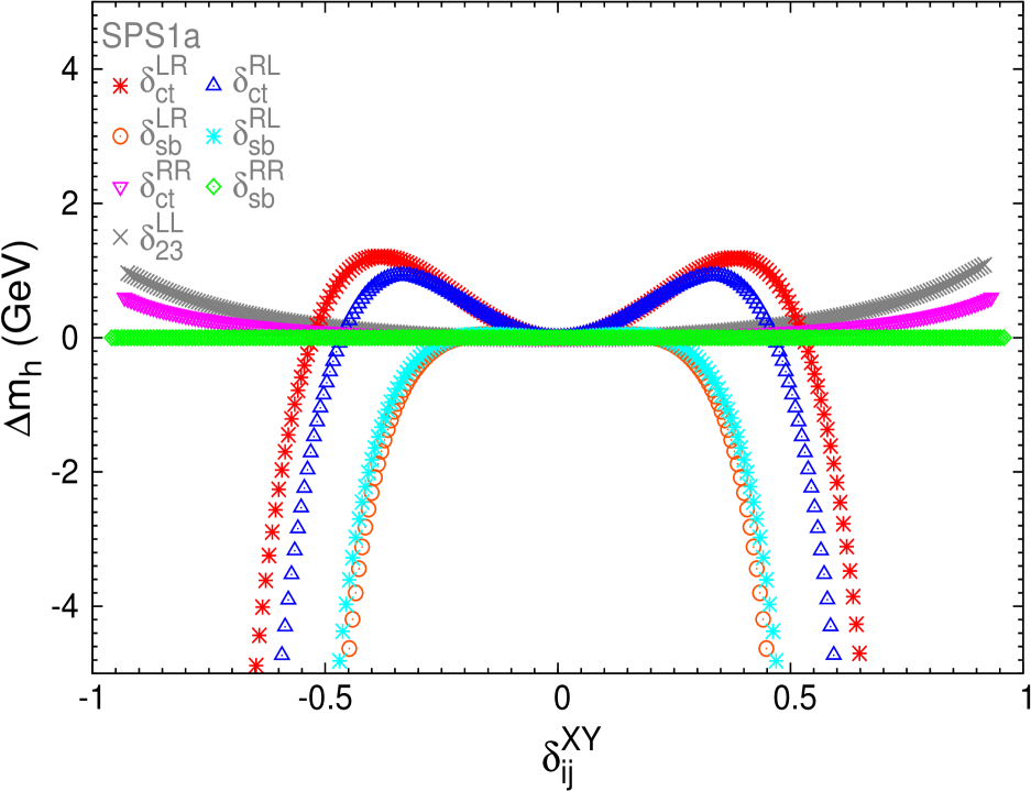
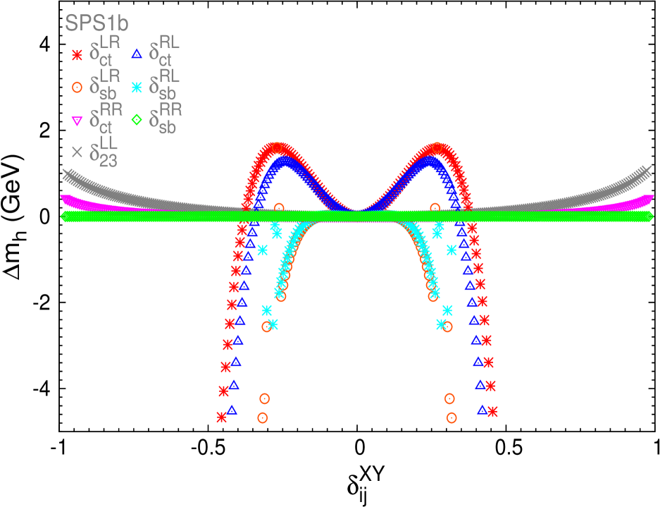
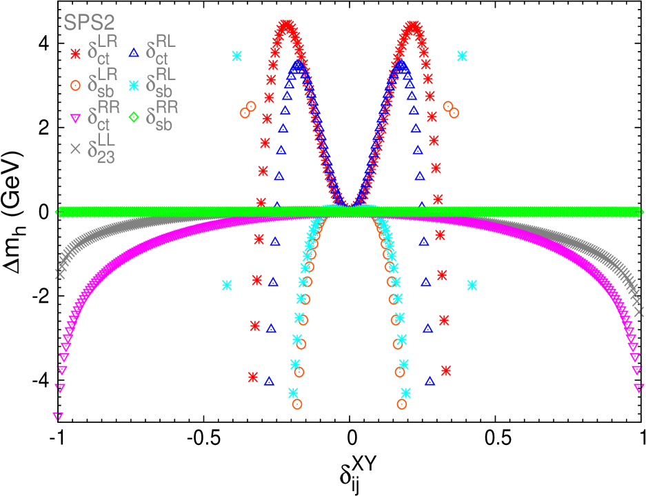
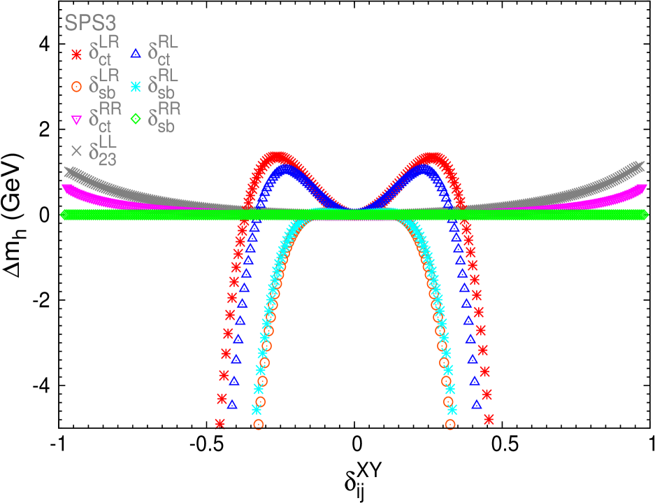
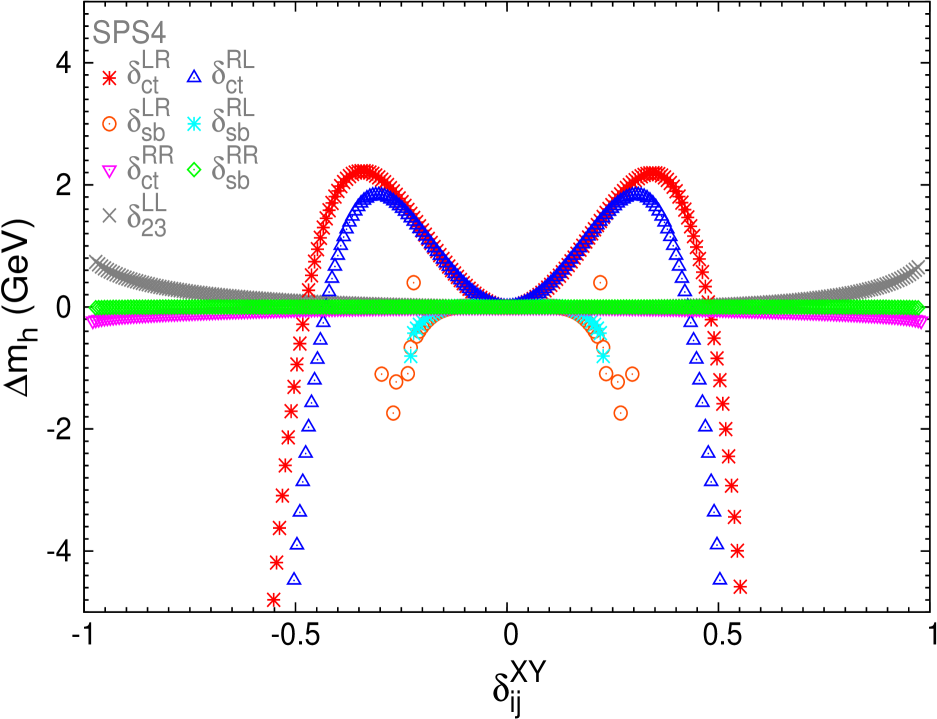
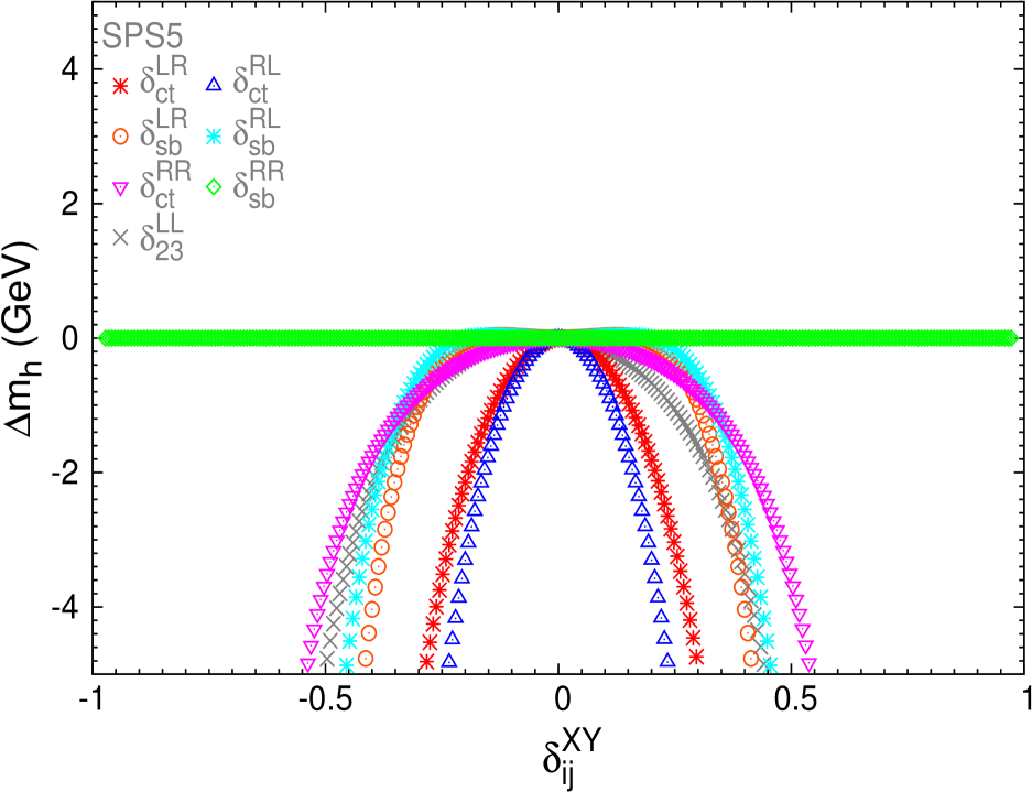
Figure 7.1: Sensitivity to the NMFV deltas in $\Delta m_{h}$ for the SPSX points of table 5.1.

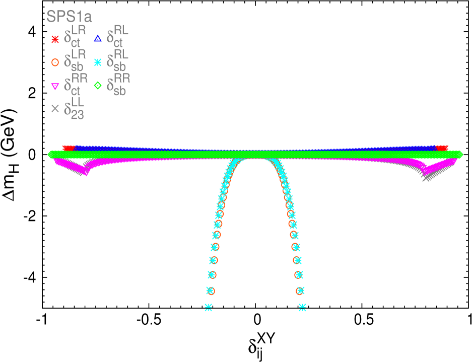
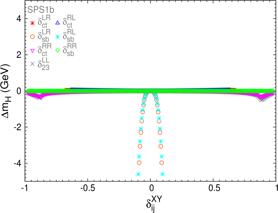
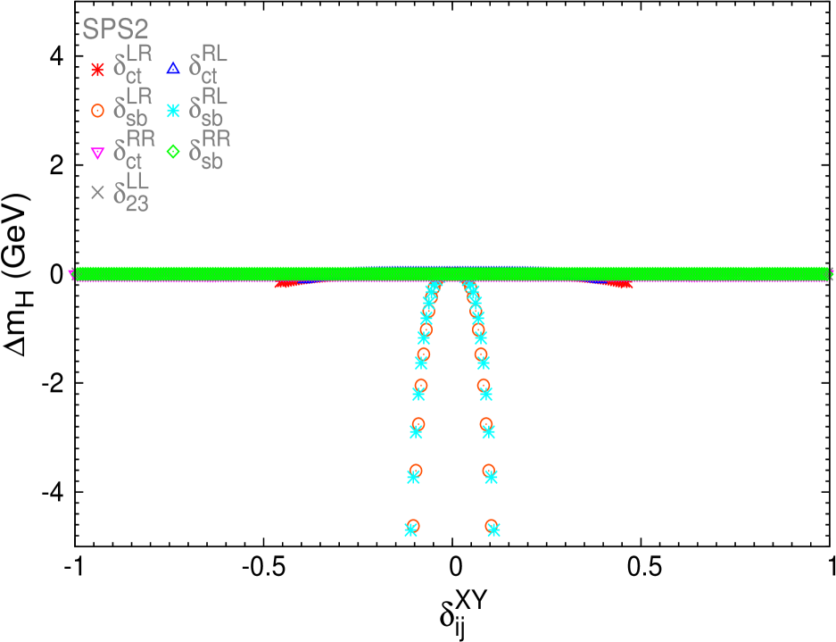
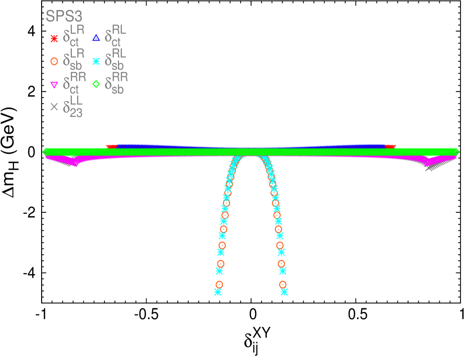
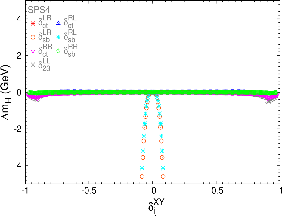
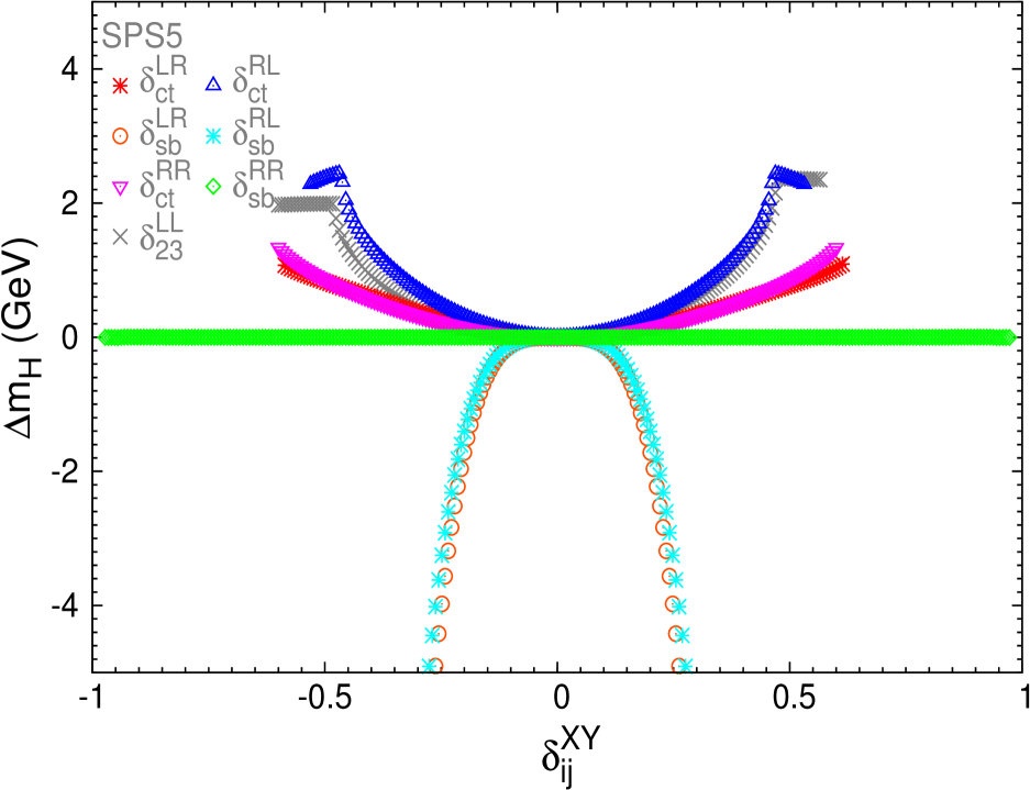
Figure 7.2: Sensitivity to the NMFV deltas in $\Delta m_{H}$ for the SPSX points of table 5.1.

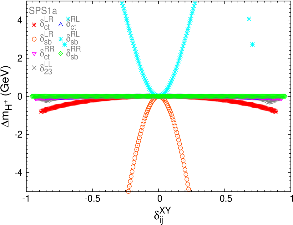
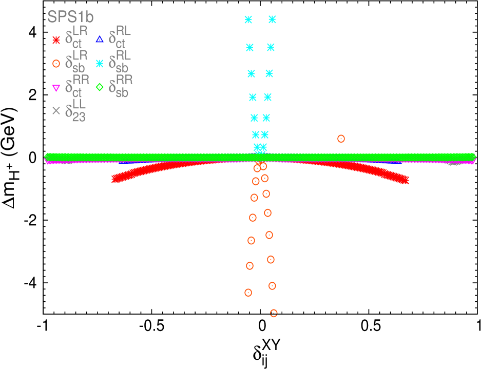
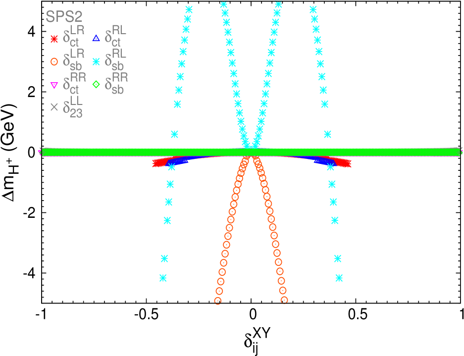
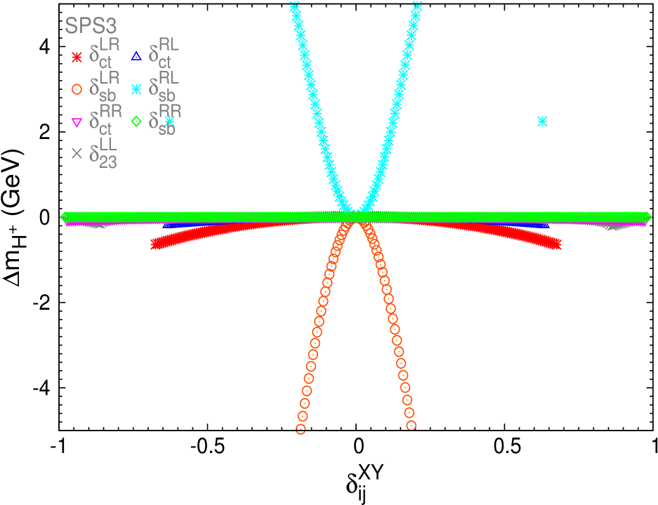
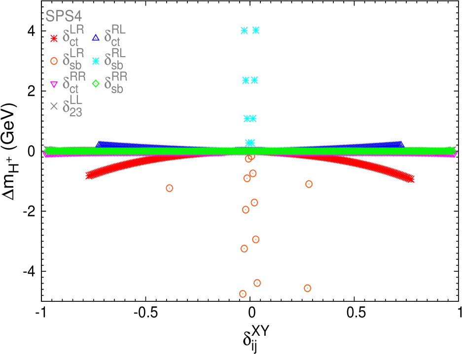
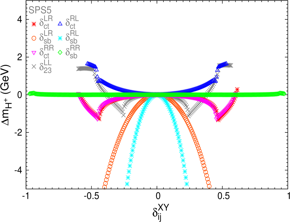
Figure 7.3: Sensitivity to the NMFV deltas in $\Delta m_{H^{\pm}}$ for the SPSX points of table 5.1.

7.3.1.2 $\Delta m_{h}$ versus two $\delta^{XY}_{ij}\neq 0$

Our previous results on the Higgs mass corrections show that the corrections to the lightest Higgs mass $\Delta m_{h}$ were negative in many of the studied cases and could be very large for some regions of the flavour changing deltas which in this pre-LHC situation were still allowed by $B$ data. These negative and large mass corrections, could lead to a prediction for the corrected one-loop mass in these kind of NMFV-SUSY scenarios, $m_{h}^{\rm NMFV}\simeq m_{h}^{\rm MSSM}+\Delta m_{h}$, which were indeed too low and already excluded by the pre-LHC data [309, 310]. Therefore, interestingly, the study of these mass corrections could be conclusive in the setting of additional restrictions on the size of some flavour changing deltas which otherwise were not bounded from $B$ data. As we will see in the post-LHC situation, both the corrections positive and negative can be relevant, and will lead to constraints in some of the deltas.

In order to explore further the size of these ‘dangerous’ mass corrections, we have computed numerically the size of $\Delta m_{h}$ as a function of two non-vanishing deltas and have looked for areas in these two dimensional plots that were allowed by $B$ data. We show in Figs. 7.5, 7.6, 7.7, 7.8, 7.9, and 7.10 the numerical results of the $\Delta m_{h}$ contour-lines in two dimensional plots, $(\delta^{LL}_{23},\delta^{XY}_{ij})$, for the respective pre-LHC points BFP, SPS2, SPS3, SPS5, VHeavyS and HeavySLightH of table 5.1.

Figure 7.4: Legend for plots of Higgs mass corrections varying two deltas simultaneously displayed in figs. 7.5, 7.6, 7.7, 7.8, 7.9 and 7.10. Each coloured area represents the disallowed region by the specified observable/s inside each box. A white area placed at the central regions of the mentioned figures represents a region allowed by the three $B$ observables. A white area placed outside the coloured areas represent regions of the parameter space that generate negative squared masses. These problematic points are consequently not shown in our plots, as we did in the previous plots. The discontinuous lines in those figures represent the contour lines for the $B$ observables corresponding to the maximum and minimum pre-LHC allowed values: dash-dot-dash for the upper bound of ${\rm BR}(B\to X_{s}\gamma)$ (Eq. (6.22)), dot-dash-dot for the lower bound of ${\rm BR}(B\to X_{s}\gamma)$ (Eq. (6.22)), dashed line for the upper bound of $\Delta M_{B_{s}}$ (Eq. (6.24)), a sequential three dotted line for the lower bound of $\Delta M_{B_{s}}$ (Eq. (6.24)), and a dotted line for the upper bound of ${\rm BR}(B_{s}\to\mu^{+}\mu^{-})$ (Eq. (6.23)).

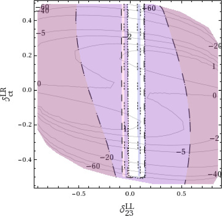
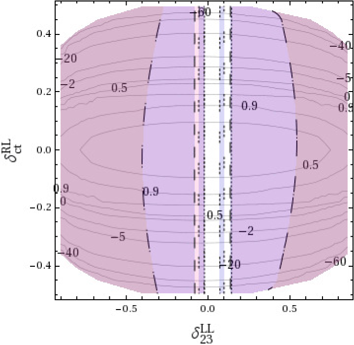
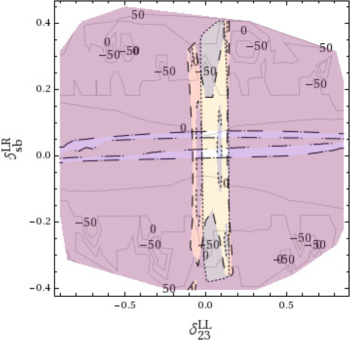
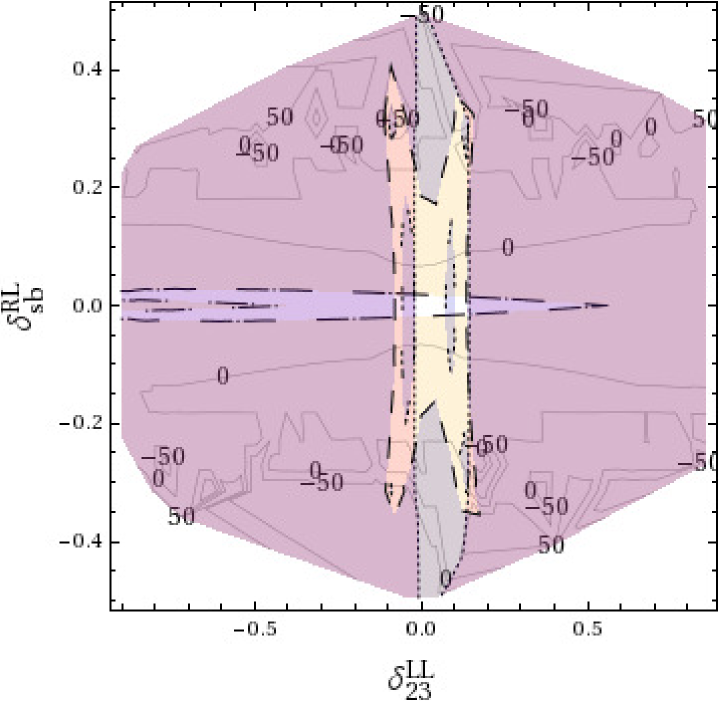
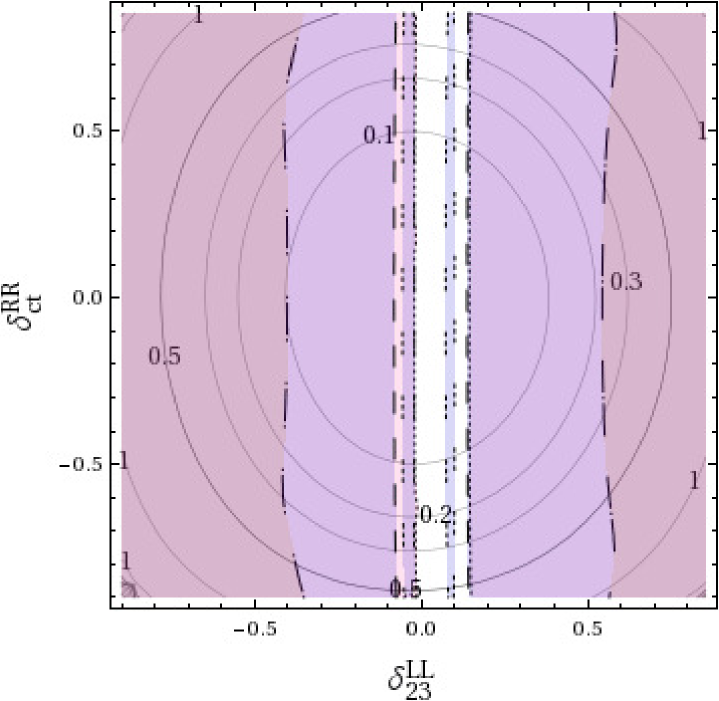
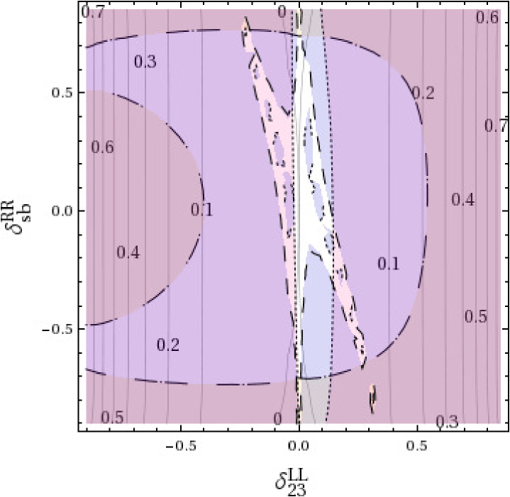
Figure 7.5: $\Delta m_{h}$ (GeV) contour lines from our two deltas analysis for BFP. The colour code for the allowed/disallowed areas by pre-LHC $B$ data is given in Fig.7.4.

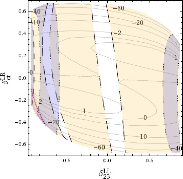
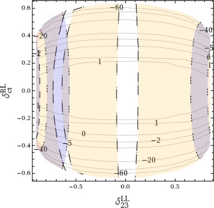
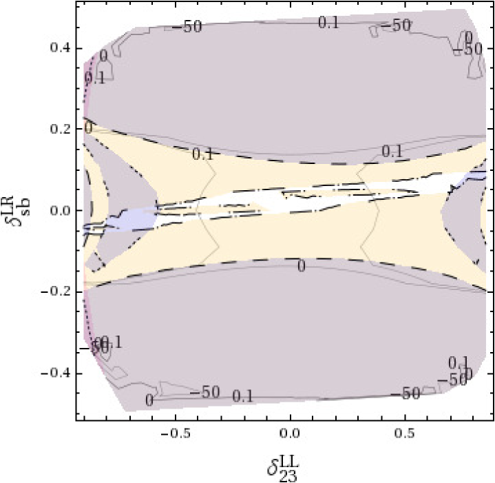
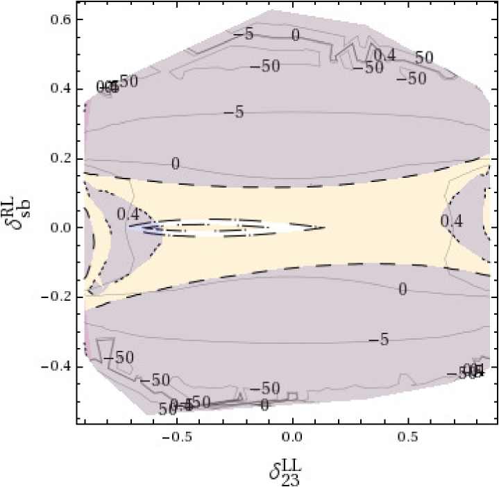
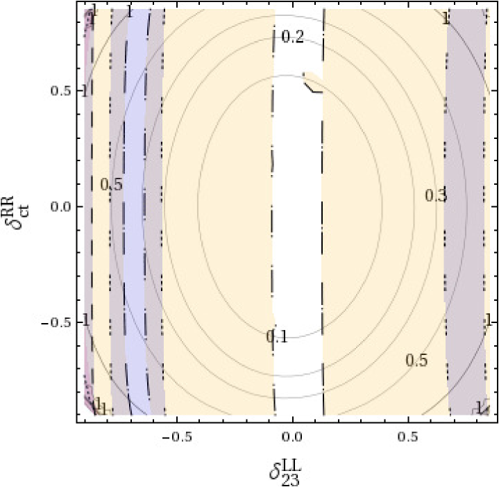
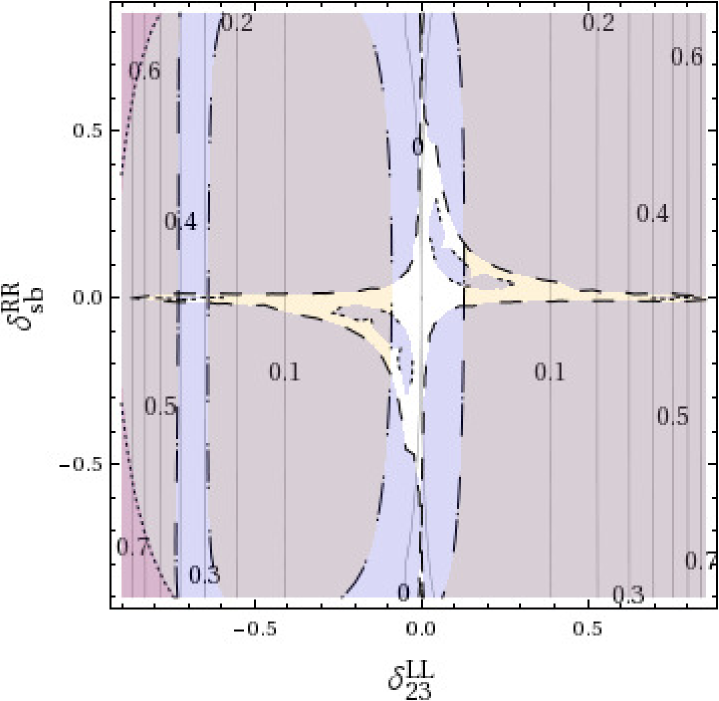
Figure 7.6: $\Delta m_{h}$ (GeV) contour lines from our two deltas analysis for SPS3. The colour code for the allowed/disallowed areas by pre-LHC $B$ data is given in Fig.7.4.

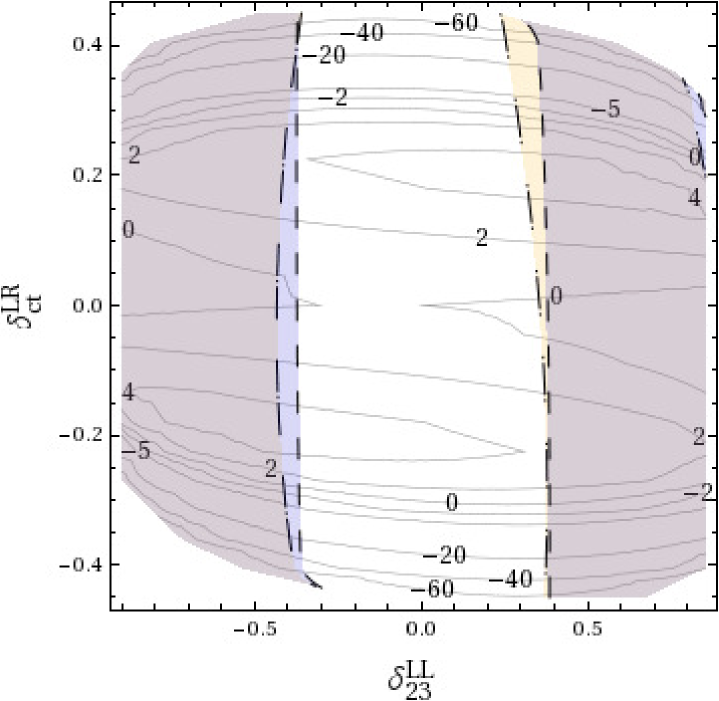
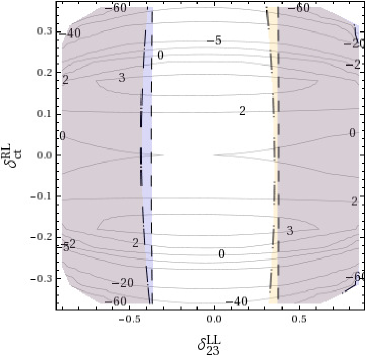
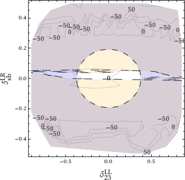
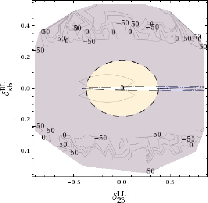
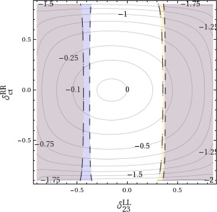
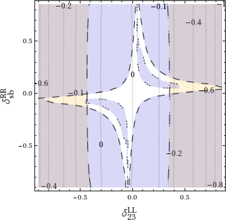
Figure 7.7: $\Delta m_{h}$ (GeV) contour lines from our two deltas analysis for SPS2. The colour code for the allowed/disallowed areas by pre-LHC $B$ data is given in Fig.7.4.

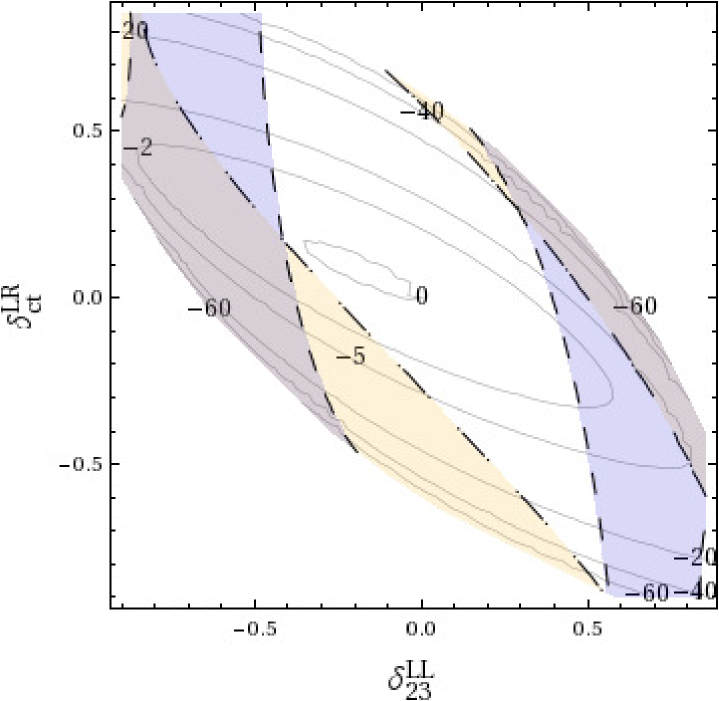
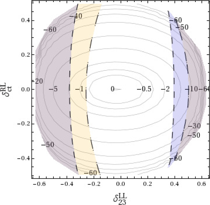
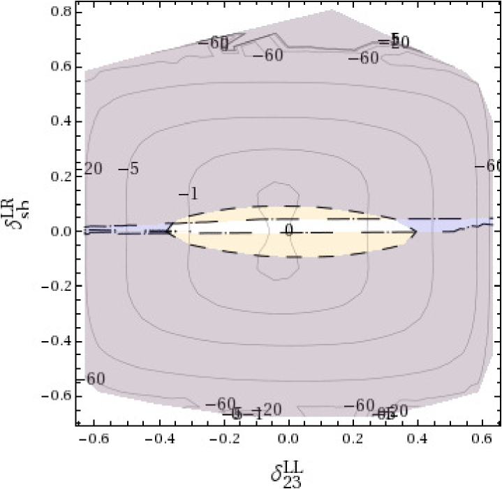
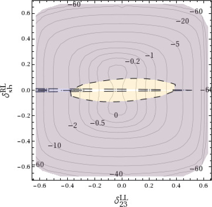
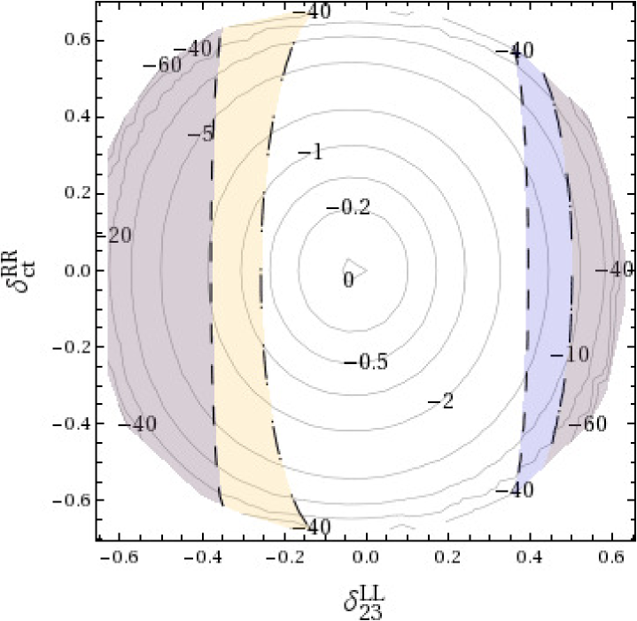
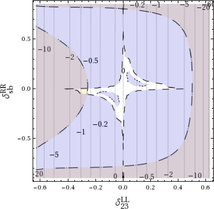
Figure 7.8: $\Delta m_{h}$ (GeV) contour lines from our two deltas analysis for SPS5. The colour code for the allowed/disallowed areas by pre-LHC $B$ data is given in Fig.7.4.

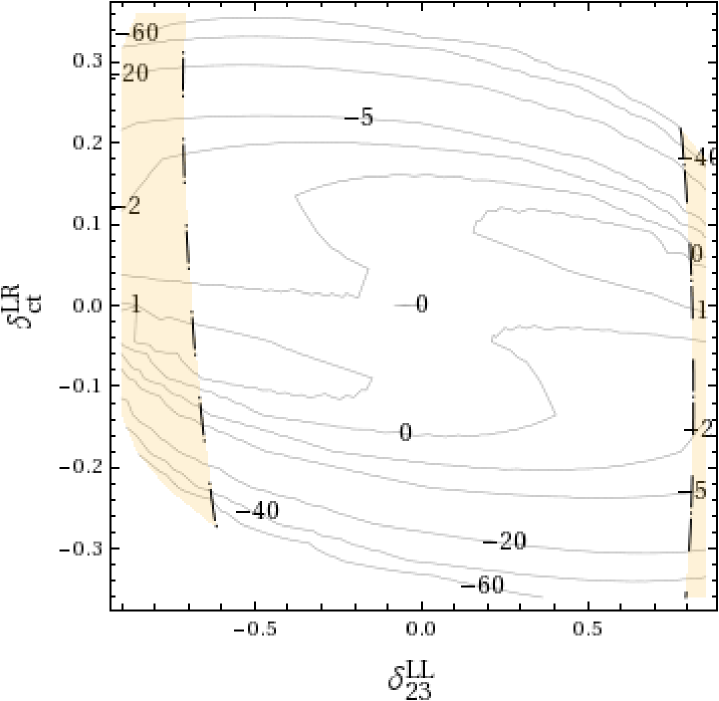
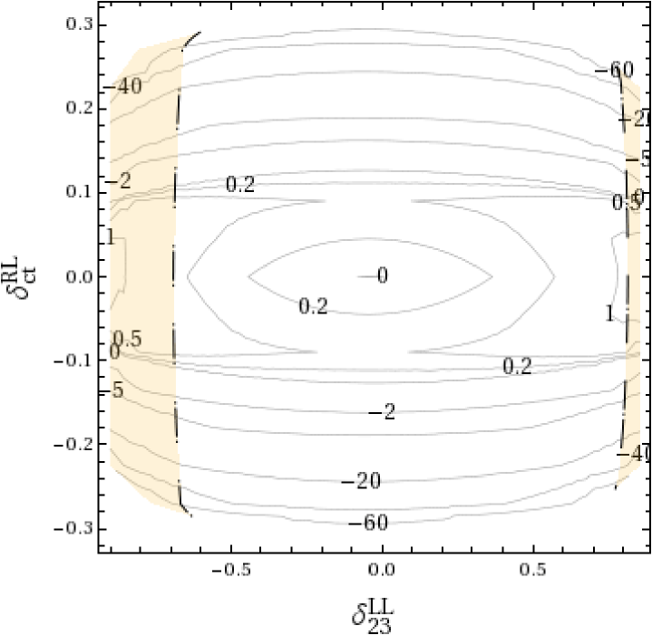
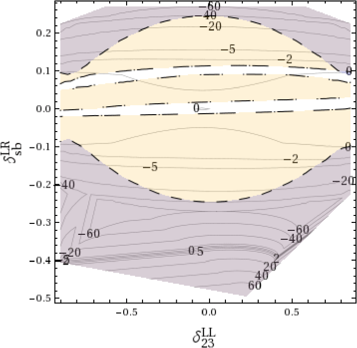
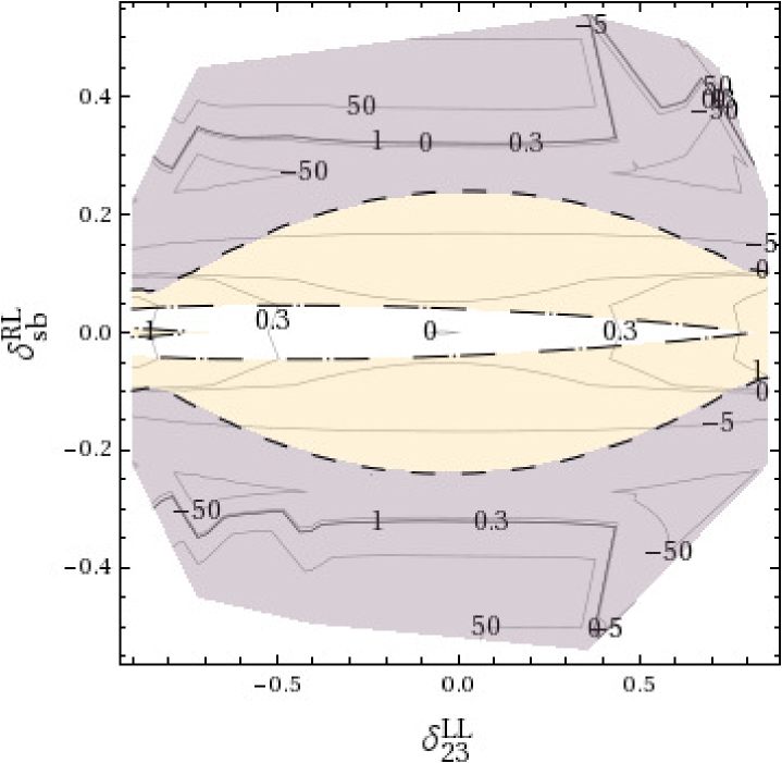
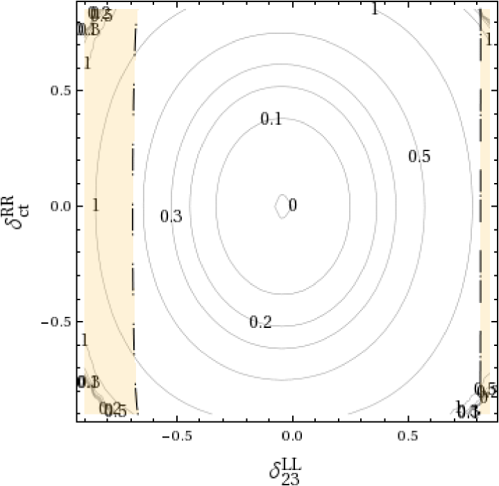
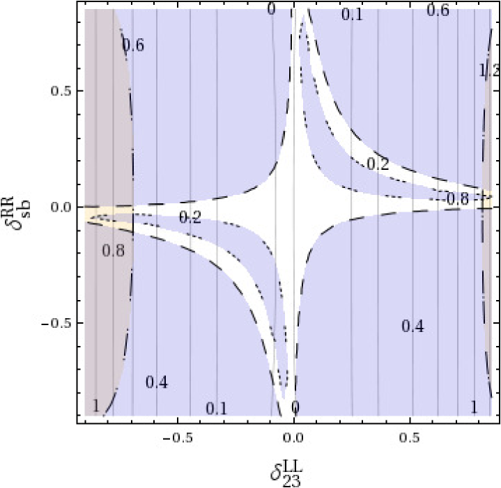
Figure 7.9: $\Delta m_{h}$ (GeV) contour lines from our two deltas analysis for VHeavyS. The colour code for the allowed/disallowed areas by pre-LHC $B$ data is given in Fig.7.4.

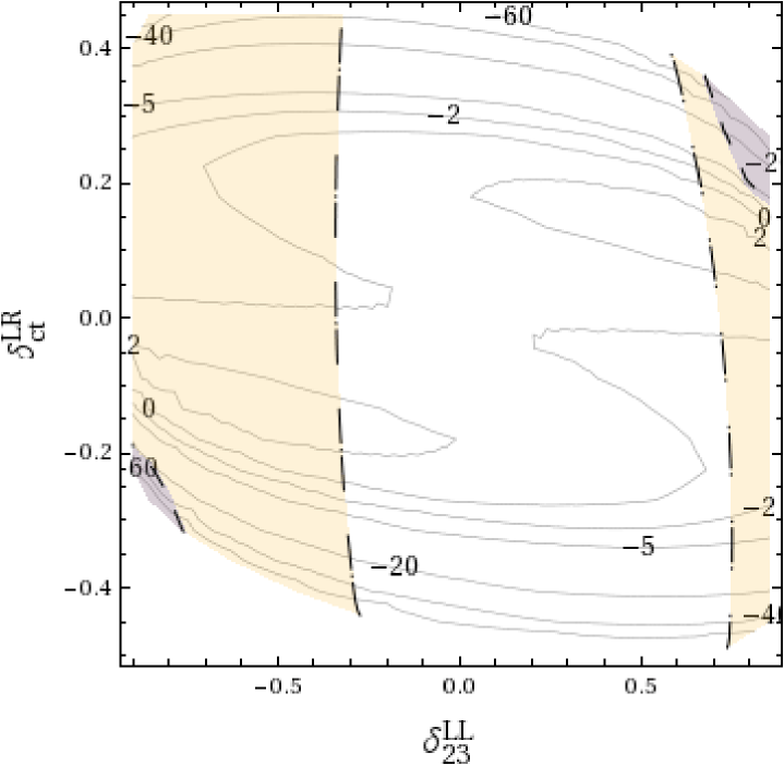
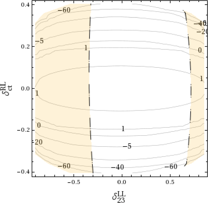
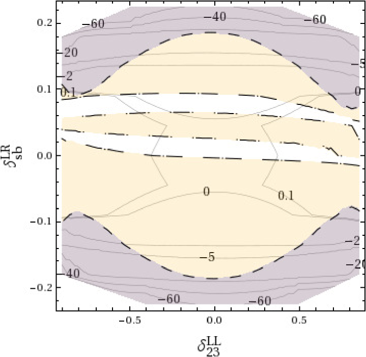
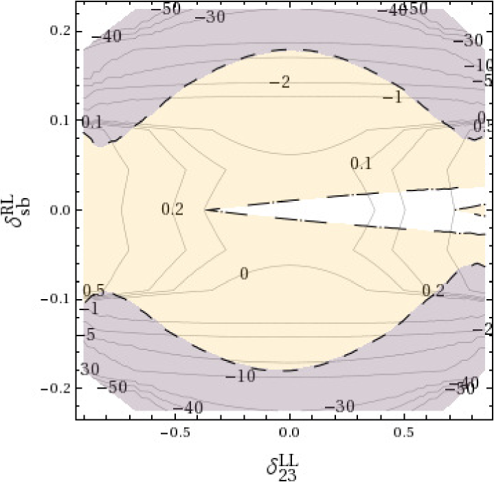
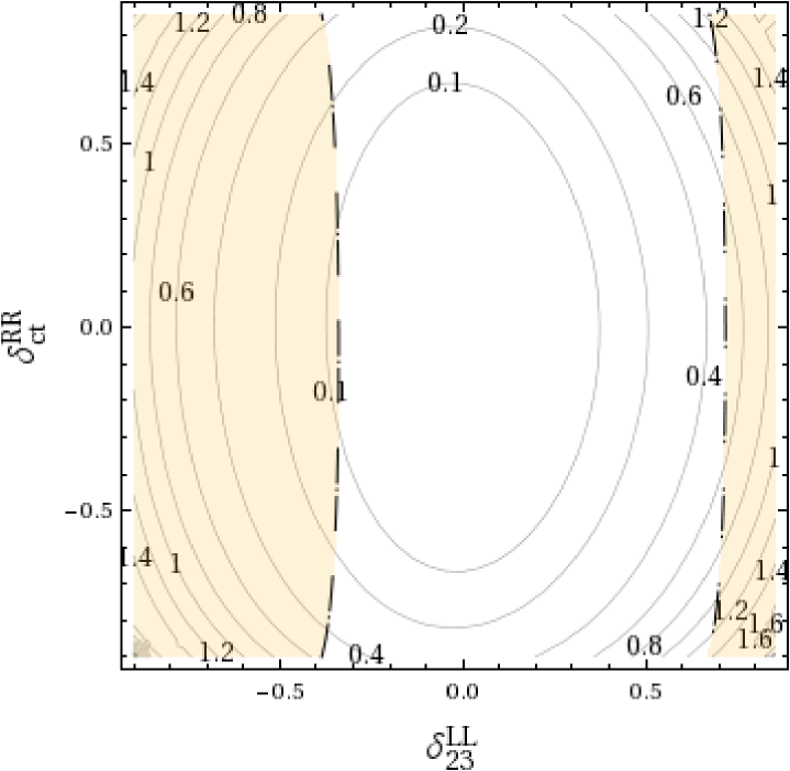
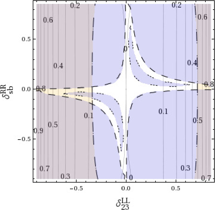
Figure 7.10: $\Delta m_{h}$ (GeV) contour lines from our two deltas analysis for HeavySLightH. The colour code for the allowed/disallowed areas by pre-LHC $B$ data is given in Fig.7.4.

We have chosen in all plots $\delta^{LL}_{23}$ as one of these non-vanishing deltas mainly because of two reasons. First, because it is one of the most frequently studied flavour changing parameters in the literature and, therefore, a convenient reference parameter. Second, because there are several well motivated SUSY scenarios, where this parameter is allowed to take the largest value, as we explained in Section 5.1.1.

In these two-dimensional figures we have included the allowed/disallowed by pre-LHC $B$ data areas that have been found by following the procedure explained in Section 6, and the allowed intervals are given in eqs.(6.22), (6.23) and (6.24). The colour code explaining the meaning of each coloured area and the codes for the discontinuous lines are given in Fig.7.4. Contour lines corresponding to mass corrections above 60 GeV or below -60 GeV have not been represented. In several scenarios the plots involving $\delta^{LR,RL}_{sb}$ show a seemingly abrupt behaviour for $|\delta^{LR,RL}_{sb}|\mathrel{\;{\hbox{\raise 1.50696pt\hbox{$>$}}\kern-3.8889pt\kern-3.8889pt\hbox{\lower 2.79857pt\hbox{$\sim$}}}\;}0.3$, corresponding to extremely large (one-loop) corrections to $m_{h}$. In general, in the case of very large one-loop corrections, in order to get a more stable result further higher order corrections would be required, as it is known from the higher-order corrections to $m_{h}$ in the MFV case (see, e.g., Ref. [240]). However, we cannot explore this possibility here. On the other hand, in order to understand the behaviour of $m_{h}$ as a function of $\delta^{LR,RL}_{sb}$ a simple analytical formula would have to be extracted from the general result. However, this is beyond the scope of this thesis.

The main conclusions from these two dimensional figures are summarized in the following:

The points that have been chosen in these plots are quite representative of all the different patterns found. The plots for SPS1a (not shown here) manifest similar patterns as those of SPS3. The plots for SPS1b (not shown here) manifest similar patterns as those of BFP. The plots for SPS4 are not included because they do not manifest any allowed areas by $B$ data.

The largest mass corrections $\Delta m_{h}$ found, being allowed by $B$ data occur in plots $(\delta^{LL}_{23},\delta^{LR}_{ct})$ and $(\delta^{LL}_{23},\delta^{RL}_{ct})$. This applies to all the studied points. They can be as large as $(-50,-100)$ GeV at $\delta^{LR}_{ct}$ or $\delta^{RL}_{ct}$ close to the upper and lower horizontal bands in these plots where $\delta^{LR}_{ct}$ or $\delta^{RL}_{ct}$ are close to $\pm 0.5$. Again these large corrections from the $LR$ and $RL$ parameters are due to the $A$-terms, as we explained at the end of Section 7.3.1.1. Comparing the different plots, it can be seen that the size of the allowed area by the pre-LHC $B$ data (the white area inside of the coloured regions) can be easily understood basically in terms of $\tan\beta$, and the heaviness of the SUSY and Higgs spectra. Generically, the plots with largest allowed regions and with largest Higgs mass corrections correspond to scenarios with low $\tan\beta=5$ and heavy spectra. Consequently, the cases of VHeavyS and HeavySLightH are the most interesting ones, exhibiting very large radiative corrections, resulting from the heavy SUSY spectra. In the case of HeavySLightH the large corrections are not only found for $\Delta m_{h}$, but also, though to a lesser extent, for the other Higgs bosons, $\Delta m_{H}$ and $\Delta m_{H^{\pm}}$ (not shown here). Consequently, in this scenario the deltas were very restricted by the mass bounds, especially by $m_{h}$.

There are also important corrections in the allowed areas of the two dimensional plots of $(\delta^{LL}_{23},\delta^{RR}_{ct})$ for some points, particularly for SPS5 (and to a lesser extent for SPS2). Here the corrections can be as large as -50 GeV in the upper and lower parts, i.e. for $\delta^{RR}_{ct}$ close to $\pm 0.5$. In the case of SPS2 they can be up to -2 GeV for this same region.

As for the remaining two-dimensional plots they do not show relevant allowed areas where the mass corrections are interestingly large.

7.3.2 Numerical results for post-LHC scenarios

After studying the phenomenology of the mass corrections with respect to the different $\delta^{XY}_{ij}$ varying the parameters of the model, we perform in this section a numerical evaluation taking into account the present experimental situation. The scenarios studied for this purpose are the ones described in Section 5.2.2.3. These scenarios are compatible with the LHC data and with all the current experimental bounds from $B$ physics and therefore have much heavier sparticles than the scenarios from the previous section.

7.3.2.1 $\Delta m_{\phi}$ versus one $\delta^{XY}_{ij}\neq 0$

In figs. 7.11, 7.12 and 7.13 there can be seen our numerical results for $\Delta m_{h}$, $\Delta m_{H}$ and $\Delta m_{H^{\pm}}$, respectively, as functions of the seven considered flavour changing deltas, $\delta^{LL}_{23}$, $\delta^{LR}_{ct}$, $\delta^{LR}_{sb}$, $\delta^{RL}_{ct}$, $\delta^{RL}_{sb}$, $\delta^{RR}_{ct}$ and $\delta^{RR}_{sb}$, which we vary in the interval $-1\leq\delta^{XY}_{ij}\leq 1$. These plots have been done for the points of table 5.2 designed considering the most up-to-date experimental measurements. This same set of points was considered in Section 6.4.2 for studying the current constraints from $B$ physics to the squark flavour mixing. Taking those into account here would lead to a reduced variation of the Higgs boson mass corrections.

The main conclusions from these new figures, taking into account what we learned from the pre-LHC points, are the following:

• General features:

  The forms of all mass corrections remain the same as in the pre-LHC studied points, being symmetric and with positive and negative corrections depending on the value of the delta. The size of the corrections however has changed, for example the positive corrections to the light Higgs boson $\Delta m_{h}$ are staying in all scenarios below 2 GeV. In contrast, the negative corrections to this boson mass, and in general all the corrections to $\Delta m_{H}$ and $\Delta m_{H^{\pm}}$ are much more steep, and reach large values with smaller values of delta than in the previous scenarios. For example, $\delta^{LR/RL}_{ct}$ can generate corrections to $\Delta m_{h}$ around 5 GeV with values of the deltas around 0.1, while in the pre-LHC scenarios that size of the corrections was reached for $\delta^{LR/RL}_{ct}$ with values around 0.5. As we commented before, the negative corrections $\Delta m_{h}$ coming from $\delta^{LR/RL}_{ct}$ can be very large, and even lead to a negative mass squared value. In these post-LHC scenarios this happens for values of the deltas around 0.3, while in the pre-LHC scenarios this happened for values between 0.5 and 0.6 depending on the point.

  There are no big differences in the behaviour of the corrections between the different points, even having different values of $\tan\beta$, except for the point S4 that has very light squarks for the third generation. We find large corrections $|\Delta m_{h}|\mathrel{\;{\hbox{\raise 1.50696pt\hbox{$>$}}\kern-3.8889pt\kern-3.8889pt\hbox{\lower 2.79857pt\hbox{$\sim$}}}\;}5\,\,\mathrm{GeV}$ for $\delta^{LR}_{sb}$, $\delta^{RL}_{sb}$, $\delta^{LR}_{ct}$ and $\delta^{RL}_{ct}$ around 0.1 and 0.2 for all the points except S4. For $\Delta m_{H}$ and $\Delta m_{H^{\pm}}$ these corrections are reached for deltas of 0.1 but only for $\delta^{LR}_{sb}$ and $\delta^{RL}_{sb}$. We find also $\Delta m_{h}$ corrections around 1 GeV for values of the deltas around 0.9 in the case of $\delta^{RR}_{ct}$ and $\delta^{LL}_{23}$, that could be relevant taking into account the future precision of the LHC and future experiments.

• Sensitivity to the various deltas:

  We find again very strong sensitivity in the three mass corrections $\Delta m_{h}$, $\Delta m_{H}$ and $\Delta m_{H^{\pm}}$, to $\delta^{LR}_{sb}$ and $\delta^{RL}_{sb}$ for all the considered points.

  In the case of $\Delta m_{h}$ there is also an important sensitivity to $\delta^{LR}_{ct}$ and $\delta^{RL}_{ct}$ in all the considered points, due to the same reasons we explained in the pre-LHC case. Also some sensitivity to $\delta^{RR}_{ct}$ and $\delta^{LL}_{23}$ is found for large values of the deltas. For the S4 point, this sensitivity is much stronger reaching large corrections.

  For $\Delta m_{H}$ in there can be seen some sensitivity to $\delta^{RR}_{ct}$, and a general sensitivity to all deltas for S4.

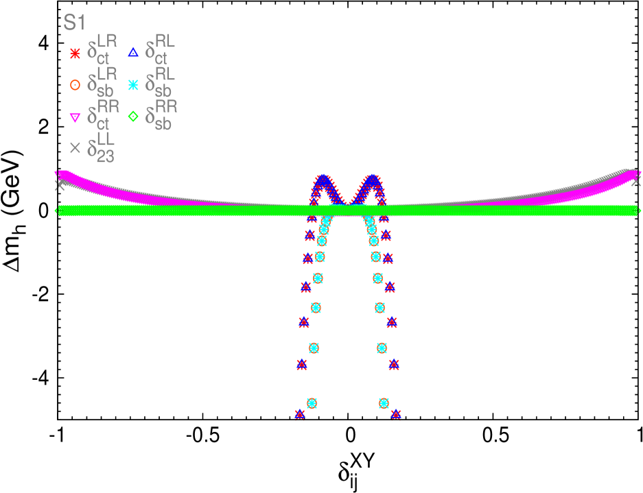
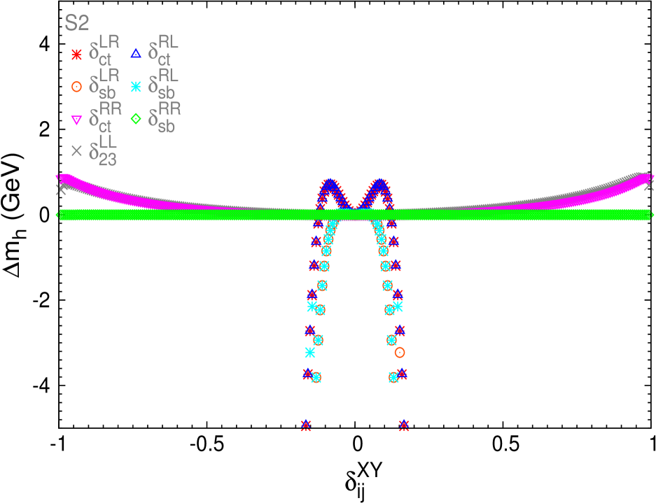
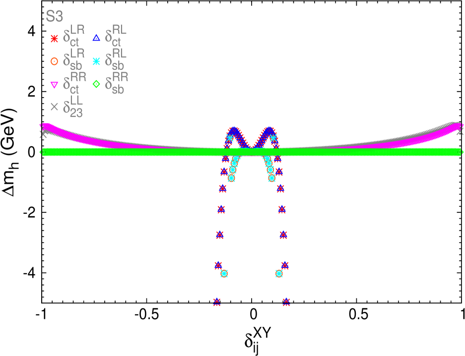
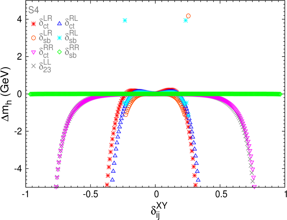
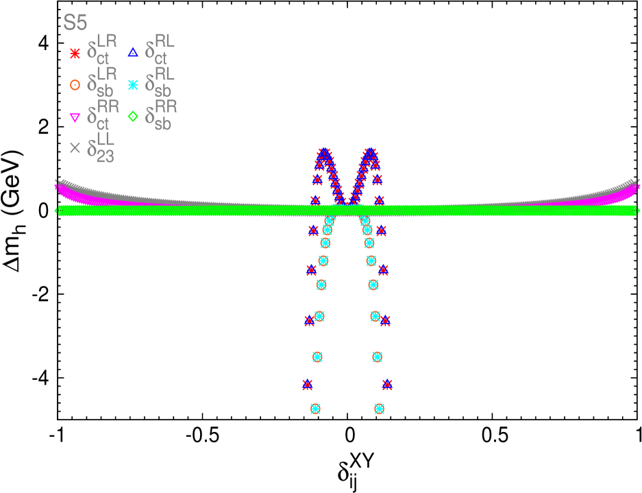
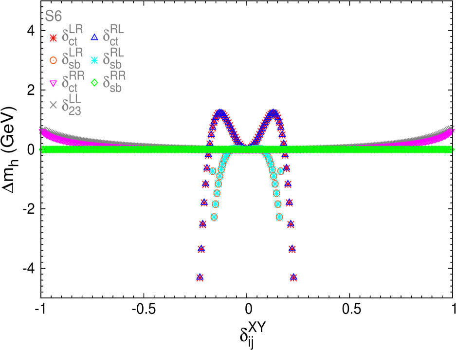
Figure 7.11: Sensitivity to the NMFV deltas in $\Delta m_{h}$ for the six post-LHC scenarios of table 5.2.

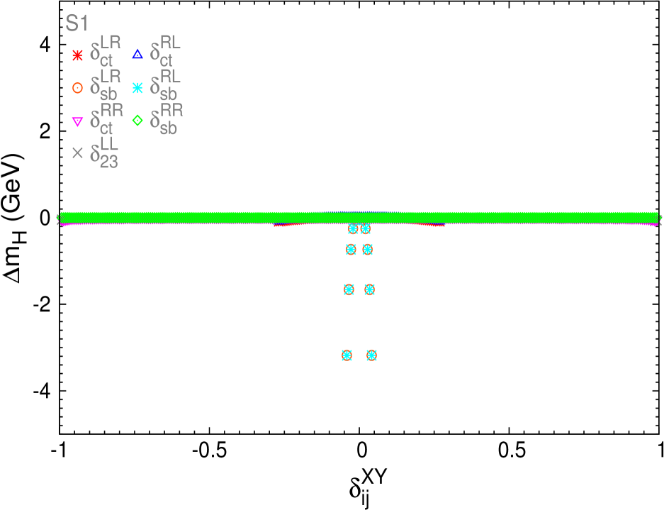
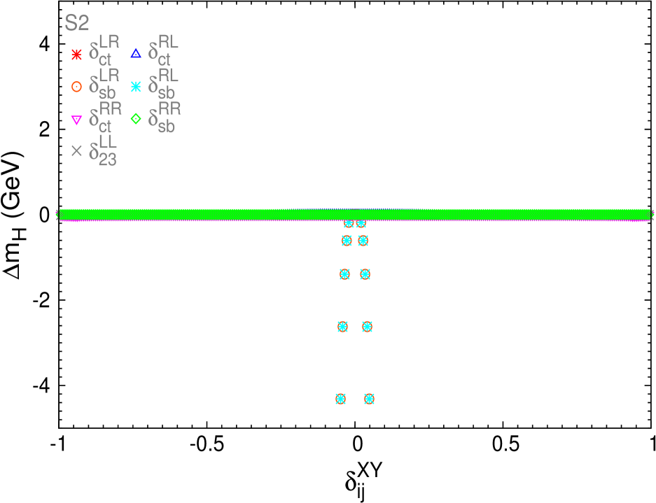
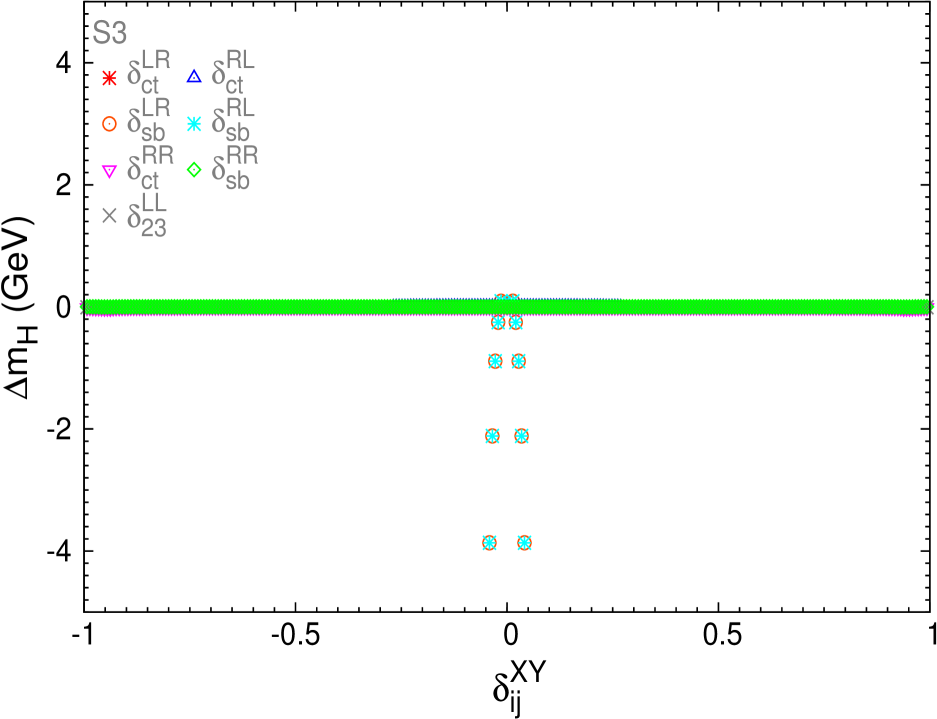
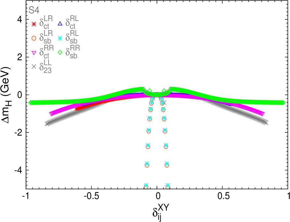
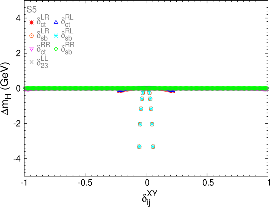
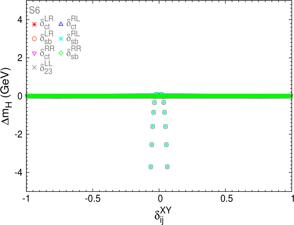
Figure 7.12: Sensitivity to the NMFV deltas in $\Delta m_{H}$ for the six post-LHC scenarios of table 5.2.

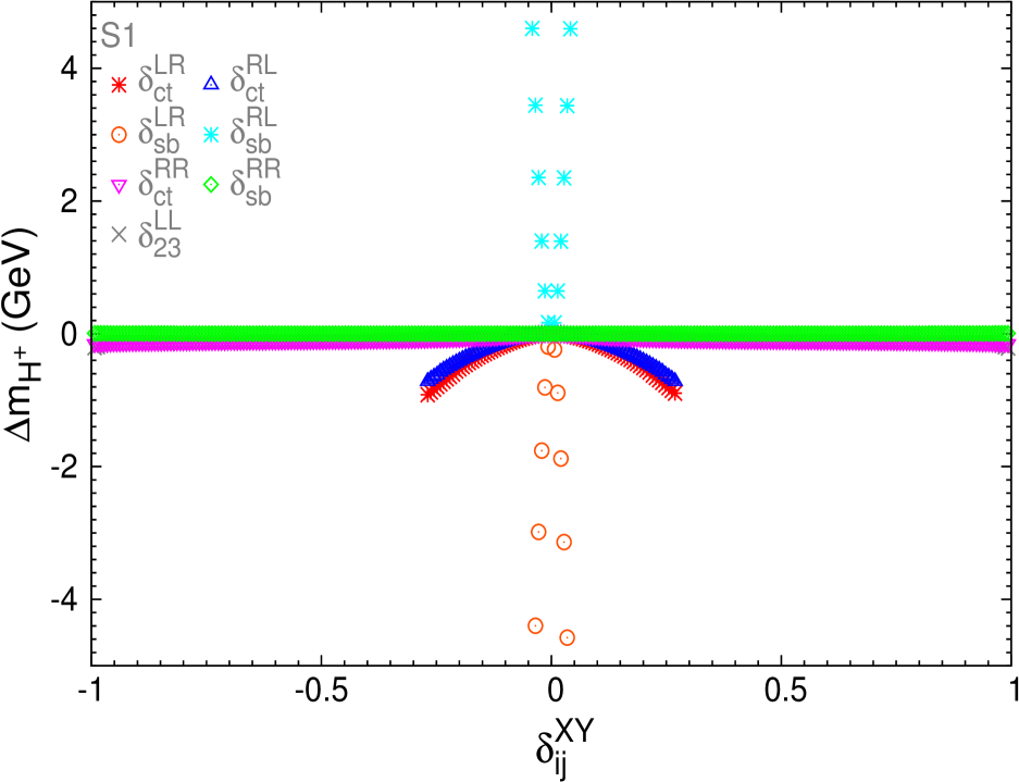
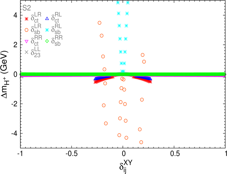
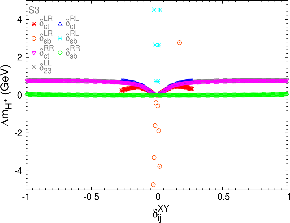
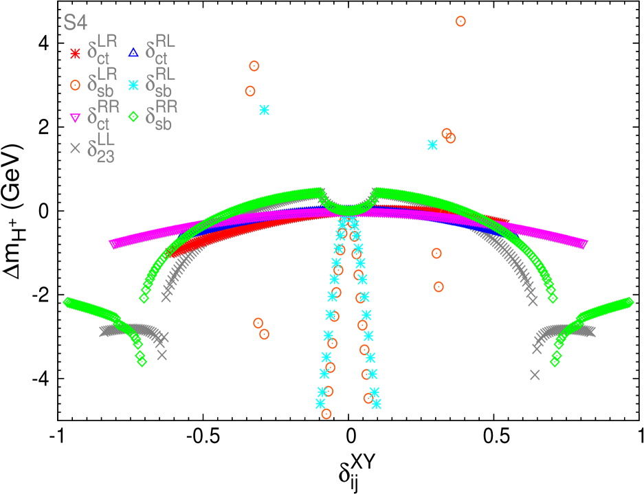
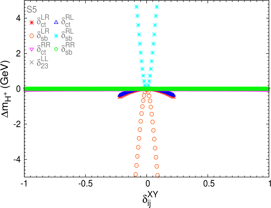
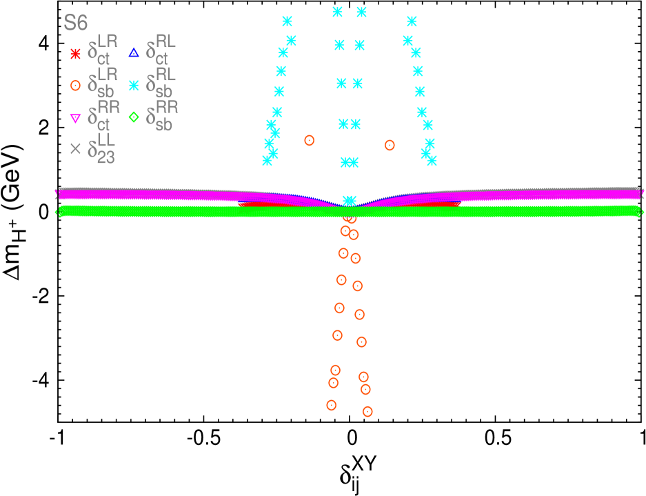
Figure 7.13: Sensitivity to the NMFV deltas in $\Delta m_{H^{\pm}}$ for the six post-LHC scenarios of table 5.2.

Chapter 8 Slepton flavour mixing effects on LFV observables

In this chapter we will perform a general study of all the flavour mixing parameters in the slepton sector, as they were introduced in Section 5.1.2. To this end, different LFV processes will be selected in the first section, relevant to each one of the flavour parameters. These processes are known to get important contributions in SUSY theories and will consist in radiative $l_{j}\to l_{i}\gamma$ [311, 312, 313, 314], leptonic $l_{j}\to 3l_{i}$ [315, 314] and semileptonic $\tau\to\mu\eta$ and $\tau\to e\eta$ LFV decays [316, 317], and conversion rates of leptons in heavy nuclei [318]. Although the radiative decays are usually the most constraining LFV processes, the leptonic and semileptonic decays are also of interest because they can be mediated by the MSSM Higgs bosons, therefore giving access to the Higgs sector parameters and, presumably, with different sensitivities to the various flavour mixing parameters than those involved in the radiative decays. Once the processes are selected, and with the scenarios that were defined in Section 5.2 we will study the sensitivity and the constraints coming from these observables to the flavour mixing parameters and the MSSM parameters, and analyze comparatively which processes are the most competitive ones.

Previous studies of general slepton mixing within the MSSM have already set upper bounds for the values of some of these flavour mixing parameters from experimental LFV searches (for a review see, for instance, [319]). Most of these studies done within the Mass Insertion Approximation focused on the LFV radiative decays [320]. Others also took into account the leptonic LFV three body decays [315], as well as the muon to electron conversion in heavy nuclei[321]. There are also some studies that focus on the chirally-enhanced loop corrections that are induced in the MSSM in presence of general sources of lepton flavour violation [322, 235]. For a recent review on LFV see, for instance, [323].

Our work will update these studies in the light of recent data, both on the most relevant LFV processes [225, 212, 227, 324, 200, 325, 326] and also in view of the collected data at LHC[252, 17, 327, 248]. Besides, our full one-loop computations for all these LFV processes have the advantage over other studies in the literature that they are done fully in the physical mass basis. Therefore we do not use the MIA and our results are valid in a wider range of the sfermion flavour mixing parameters. The selected scenarios are all compatible with LHC data. In particular these scenarios have relatively heavy SUSY spectra, which are naturally in agreement with the present MSSM particle mass bounds (although substantially lower masses, especially in the electroweak sector, are allowed by LHC data). Furthermore the selected scenarios are chosen such that the light ${\cal CP}$-even MSSM Higgs mass is around $125-126\,\,\mathrm{GeV}$ and thus in agreement with the Higgs boson discovery [252]. In addition we require that our selected MSSM scenarios give a prediction for the muon anomalous magnetic moment, $(g-2)_{\mu}$, in agreement with current data [245].

The results in this chapter have been published in [73].

8.1 Study of LFV processes

The general slepton flavour mixing introduced in Section 5.1.2 produce interactions among mass eigenstates of different generations, therefore changing flavour. In the physical basis for leptons $l_{i}$ ($i=1,2,3$), sleptons $\tilde{l}_{X}$ ($X=1,..,6$), sneutrinos $\tilde{\nu}_{X}$ ($X=1,2,3$), neutralinos ${\tilde{\chi}}_{A}^{0}$ ($A=1,2,3,4$), charginos ${\tilde{\chi}}_{A}^{\pm}$ ($A=1,2$) and Higgs bosons, $H_{p}\,\,\,(p=1,2,3)=h^{0},H^{0},A^{0}$, one gets generically non-vanishing couplings for intergenerational interactions like, for instance: ${\tilde{\chi}}_{A}^{0}l_{i}{\tilde{l}}_{X}$, ${\tilde{\chi}}_{A}^{\pm}l_{i}{\tilde{\nu}}_{X}$, $Z\tilde{l}_{X}\tilde{l}_{Y}$, $H_{p}\tilde{l}_{X}\tilde{l}_{Y}$ and $H_{p}\tilde{\nu}_{X}\tilde{\nu}_{Y}$. When these interactions appear in loop-induced processes they can then mediate LFV processes involving leptons of different flavours $l_{i}$ and $l_{j}$, with $i\neq j$, in the external states. The dependence of the LFV rates for these processes on the previously introduced $\delta^{AB}_{ij}$ parameters then appears both in the values of the physical slepton and sneutrino masses, and in the values of these intergenerational couplings via the rotation matrices $R^{\tilde{l}}$ and $R^{\tilde{\nu}}$. For the present work, we use the set of Feynman rules for these and other relevant couplings among mass eigenstates, as summarized in Refs. [315, 318].

8.1.1 Selected LFV processes

Our selection of LFV processes is driven by the requirement that we wish to determine the constraints on all the slepton flavour mixing parameters by studying different kinds of one-loop LFV vertices involving $l_{i}$ and $l_{j}$ with $i\neq j$ in the external lines. In particular we want to study the sensitivity to the $\delta^{AB}_{ij}$’s in the most relevant (three-point) LFV one-loop vertices, which are: the vertex with a photon, $(l_{i}l_{j}\gamma)_{\rm 1-loop}$, the vertex with a $Z$ gauge boson, $(l_{i}l_{j}Z)_{\rm 1-loop}$ and the vertices with the Higgs bosons, $(l_{i}l_{j}h^{0})_{\rm 1-loop}$, $(l_{i}l_{j}H^{0})_{\rm 1-loop}$ and $(l_{i}l_{j}A^{0})_{\rm 1-loop}$. This leads us to single out some specific LFV processes where these one-loop generated LFV vertices play a relevant role. We have chosen the following subset of LFV processes, all together involving these particular LFV one-loop vertices:

• Radiative LFV decays: $\mu\to e\gamma$, $\tau\to e\gamma$ and $\tau\to\mu\gamma$. These are sensitive to the $\delta^{AB}_{ij}$’s via the $(l_{i}l_{j}\gamma)_{\rm 1-loop}$ vertices with a real photon.

• Leptonic LFV decays: $\mu\to 3e$, $\tau\to 3e$ and $\tau\to 3\mu$. These are sensitive to the $\delta^{AB}_{ij}$’s via the $(l_{i}l_{j}\gamma)_{\rm 1-loop}$ vertices with a virtual photon, via the $(l_{i}l_{j}Z)_{\rm 1-loop}$ vertices with a virtual $Z$, and via the $(l_{i}l_{j}h^{0})_{\rm 1-loop}$, $(l_{i}l_{j}H^{0})_{\rm 1-loop}$ and $(l_{i}l_{j}A^{0})_{\rm 1-loop}$ vertices with virtual Higgs bosons.

• Semileptonic LFV tau decays: $\tau\to\mu\eta$ and $\tau\to e\eta$. These are sensitive to the $\delta^{AB}_{ij}$’s via $(\tau\mu A^{0})_{\rm 1-loop}$ and $(\tau eA^{0})_{\rm 1-loop}$ vertices, respectively, with a virtual $A^{0}$, and via $(\tau\mu Z)_{\rm 1-loop}$ and $(\tau eZ)_{\rm 1-loop}$ vertices, respectively with a virtual $Z$.

• Conversion of $\mu$ into $e$ in heavy nuclei: These are sensitive to the $\delta^{AB}_{ij}$’s via the $(\mu e\gamma)_{\rm 1-loop}$ vertex with a virtual photon, via the $(\mu eZ)_{\rm 1-loop}$ vertex with a virtual $Z$, and via the $(\mu eh^{0})_{\rm 1-loop}$ and $(\mu eH^{0})_{\rm 1-loop}$ vertices with a virtual $h^{0}$ and $H^{0}$ Higgs boson, respectively.

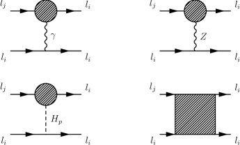
Figure 8.1: Generic one-loop diagrams contributing to LFV processes: 1) $l_{j}\to l_{i}\gamma$; 2) $l_{j}\to 3l_{i}$, mediated by $\gamma$ and $Z$ gauge bosons, by $H_{p}=h^{0},H^{0},A^{0}$ Higgs bosons and by boxes; 3) $\tau\to\mu\eta$ and $\tau\to e\eta$, mediated by $A^{0}$ Higgs boson and by $Z$ gauge boson; 4) $\mu-e$ conversion in nuclei, mediated by $\gamma$, and $Z$ gauge bosons, by $H_{p}=h^{0},H^{0}$ Higgs bosons, and by boxes.

The generic one-loop diagrams contributing to all the LFV processes above, are summarized in Fig.8.1. These include the $\gamma$-mediated diagrams, the $Z$-mediated diagrams (the $Z$-penguin diagrams in $l_{j}\to 3l_{i}$ were also studied in [328]), and the $h^{0}$, $H^{0}$ and $A^{0}$-mediated diagrams. The generic one-loop box diagrams are also shown in this figure. These also include the $\delta^{AB}_{ij}$’s but their sensitivities to these parameters are much lower than via the above quoted three-point vertices. They are, however, included in our analytical results and in our numerical evaluation.

For our forthcoming numerical analysis of these LFV processes we have implemented the full one-loop formulas into our private Fortran code. The analytical results are taken from various publications: Ref. [315] for ${\rm BR}(l_{j}\to 3l_{i})$ and ${\rm BR}(l_{j}\to l_{i}\gamma)$, Ref. [316] for ${\rm BR}(\tau\to\mu\eta)$ and ${\rm BR}(\tau\to e\eta)$, and Ref. [318] for the $\mu-e$ conversion rate in heavy nuclei, relative to the muon capture rate ${\rm CR}(\mu-e,{\rm Nuclei})$. Following the same procedure of [316] we use Chiral Perturbation Theory for the needed hadronization of quark bilinears involved in the quark-level $\tau\to\mu qq^{\prime}$ and $\tau\to eqq^{\prime}$ decays that lead the $\eta$ particle in the final state. Our treatment of the heavy nuclei and the proper approximations to go from the LFV amplitudes at the parton level to the LFV rates at the nuclear level are described in [318]. For brevity, we omit to explicit here all these needed formulas for the computation of the LFV rates and refer the reader to the above quoted references for the details.

The list of specific one-loop diagrams contributing to the relevant $(l_{i}l_{j}\gamma)_{\rm 1-loop}$, $(l_{i}l_{j}Z)_{\rm 1-loop}$ $(l_{i}l_{j}h^{0})_{\rm 1-loop}$, $(l_{i}l_{j}H^{0})_{\rm 1-loop}$ and $(l_{i}l_{j}A^{0})_{\rm 1-loop}$ vertices can also be found in Refs. [315, 318]. The main contributions come from the loops with charginos/sneutrinos and with neutralinos/sleptons. This will be relevant for the analytical interpretation of our results below.

8.1.2 The MIA basic reference formulas

For completeness, and in order to get a better understanding of the forthcoming full one-loop results leading to the maximal allowed deltas and their behaviour with the relevant MSSM parameters, we include in this section the main formulas for the LFV radiative decays within the Mass Insertion Approximation that we take from Ref. [321]. These are simple formulas and illustrate clearly the qualitative behaviour of the LFV rates with all the deltas and all the MSSM parameters. The branching ratios of the radiative $l_{j}\to l_{i}\gamma$ decays, with $ji=21$, $31$ and $32$, are:

$${\rm BR}(l_{j}\to l_{i}\gamma) = \frac{\alpha}{4}(\frac{m_{l_{j}}^{5}}{\Gamma_{l_{j}}})\left(|(A_{ij}^{L})|^{2}+|(A_{ij}^{R})|^{2}\right)$$ (8.1)

where $\Gamma_{l_{j}}$ is the total ${l_{j}}$ width, and the amplitudes, in the single delta insertion approximation, are given by [321]:

$$(A_{ij}^{L})_{\rm MIA} = \frac{\alpha_{2}}{4\pi}\Delta^{LL}_{ij}\left[\frac{f_{1n}(a_{L2})+f_{1c}(a_{L2})}{m_{\tilde{L}}^{4}}+\frac{\mu M_{2}\tan\beta}{(M_{2}^{2}-\mu^{2})}\frac{(f_{2n}(a_{L2},b_{L})+f_{2c}(a_{L2},b_{L}))}{m_{\tilde{L}}^{4}}\right]$$ (8.2)

$$+ \frac{\alpha_{1}}{4\pi}\Delta^{LL}_{ij}\left[\frac{f_{1n}(a_{L})}{m_{\tilde{L}}^{4}}+\mu M_{1}\tan\beta\left(\frac{-f_{2n}(a_{L},b_{L})}{m_{\tilde{L}}^{4}(M_{1}^{2}-\mu^{2})}+\frac{2f_{2n}(a_{L})}{m_{\tilde{L}}^{4}(m_{\tilde{R}}^{2}-m_{\tilde{L}}^{2})}\right)\right]$$

$$+ \frac{\alpha_{1}}{4\pi}\Delta^{LL}_{ij}\left[\frac{\mu M_{1}\tan\beta}{(m_{\tilde{R}}^{2}-m_{\tilde{L}}^{2})^{2}}\left(\frac{f_{3n}(a_{R})}{m_{\tilde{R}}^{2}}-\frac{f_{3n}(a_{L})}{m_{\tilde{L}}^{2}}\right)\right]$$

$$+ \frac{\alpha_{1}}{4\pi}\Delta^{LR}_{ij}\left[\frac{1}{(m_{\tilde{L}}^{2}-m_{\tilde{R}}^{2})}\left(\frac{M_{1}}{m_{l_{j}}}\right)\left(\frac{f_{3n}(a_{R})}{m_{\tilde{R}}^{2}}-\frac{f_{3n}(a_{L})}{m_{\tilde{L}}^{2}}\right)\right]$$

and

$$(A_{ij}^{R})_{\rm MIA} = \frac{\alpha_{1}}{4\pi}\Delta^{RR}_{ij}\left[\frac{4f_{1n}(a_{R})}{m_{\tilde{R}}^{4}}+\mu M_{1}\tan\beta\left(\frac{2f_{2n}(a_{R},b_{R})}{m_{\tilde{R}}^{4}(M_{1}^{2}-\mu^{2})}+\frac{2f_{2n}(a_{R})}{m_{\tilde{R}}^{4}(m_{\tilde{L}}^{2}-m_{\tilde{R}}^{2})}\right)\right]$$ (8.3)

$$+ \frac{\alpha_{1}}{4\pi}\Delta^{RR}_{ij}\left[\frac{\mu M_{1}\tan\beta}{(m_{\tilde{L}}^{2}-m_{\tilde{R}}^{2})^{2}}\left(\frac{f_{3n}(a_{L})}{m_{\tilde{L}}^{2}}-\frac{f_{3n}(a_{R})}{m_{\tilde{R}}^{2}}\right)\right]$$

$$+ \frac{\alpha_{1}}{4\pi}\Delta^{RL}_{ij}\left[\frac{1}{(m_{\tilde{R}}^{2}-m_{\tilde{L}}^{2})}\left(\frac{M_{1}}{m_{l_{j}}}\right)\left(\frac{f_{3n}(a_{L})}{m_{\tilde{L}}^{2}}-\frac{f_{3n}(a_{R})}{m_{\tilde{R}}^{2}}\right)\right]~{},$$

where $\alpha_{1}=(5/3)(\alpha/\cos^{2}\theta_{W})$, $\alpha_{2}=(\alpha/\sin^{2}\theta_{W})$, $a_{L2}=M_{2}^{2}/m_{\tilde{L}}^{2}$, $a_{L}=M_{1}^{2}/m_{\tilde{L}}^{2}$, $a_{R}=M_{1}^{2}/m_{\tilde{R}}^{2}$, $b_{L}=\mu^{2}/m_{\tilde{L}}^{2}$, $b_{R}=\mu^{2}/m_{\tilde{R}}^{2}$, $\Delta^{AB}_{ij}=\delta^{AB}_{ij}m_{\tilde{A}}m_{\tilde{B}}$ and $m_{\tilde{L}}$ and $m_{\tilde{R}}$ are the average slepton masses in the ${\tilde{L}}$ and ${\tilde{R}}$ slepton sectors, respectively. The $f_{in}$’s and $f_{ic}$’s are loop functions from neutralinos and charginos contributions, respectively, given by:

$$f_{1n}(a) = \frac{-17a^{3}+9a^{2}+9a-1+6a^{2}(a+3)\ln a}{24(1-a)^{5}}~{},$$

$$f_{2n}(a) = \frac{-5a^{2}+4a+1+2a(a+2)\ln a}{4(1-a)^{4}}~{},$$

$$f_{3n}(a) = \frac{1+2a\ln a-a^{2}}{2(1-a)^{3}}~{},$$

$$f_{1c}(a) = \frac{-a^{3}-9a^{2}+9a+1+6a(a+1)\ln a}{6(1-a)^{5}}~{},$$

$$f_{2c}(a) = \frac{-a^{2}-4a+5+2(2a+1)\ln a}{2(1-a)^{4}}~{},$$

$$f_{2n}(a,b) = f_{2n}(a)-f_{2n}(b)~{},$$

$$f_{2c}(a,b) = f_{2c}(a)-f_{2c}(b)~{}.$$ (8.4)

It is also very illustrative to compare the forthcoming results with those of the MIA for the case of equal mass scales, $m_{\tilde{L}}=m_{\tilde{R}}=\mu=M_{2}=M_{1}\equiv m_{S}$. From the previous formulas we get:

$$(A_{ij}^{L})_{\rm MIA} = \frac{\alpha_{2}}{4\pi}\delta^{LL}_{ij}\left[\frac{1}{240}\frac{1}{m_{S}^{2}}+\tan\beta\frac{1}{15}\frac{1}{m_{S}^{2}}\right]$$ (8.5)

$$+ \frac{\alpha_{1}}{4\pi}\delta^{LL}_{ij}\left[\frac{-1}{80}\frac{1}{m_{S}^{2}}+\tan\beta\frac{1}{12}\frac{1}{m_{S}^{2}}\right]$$

$$+ \frac{\alpha_{1}}{4\pi}\delta^{LR}_{ij}\left[\frac{1}{m_{S}m_{l_{j}}}\right]$$

and

$$(A_{ij}^{R})_{\rm MIA} = \frac{\alpha_{1}}{4\pi}\delta^{RR}_{ij}\left[\frac{-1}{20}\frac{1}{m_{S}^{2}}-\tan\beta\frac{1}{60}\frac{1}{m_{S}^{2}}\right]$$ (8.6)

$$+ \frac{\alpha_{1}}{4\pi}\delta^{RL}_{ij}\left[\frac{1}{m_{S}m_{l_{j}}}\right]~{}.$$

In all these basic MIA formulas (see also [313]) one can see clearly the scaling of the BRs with all the deltas, in the single mass insertion approximation, and with the most relevant parameters for the present study, namely, the common/average SUSY mass $m_{S}$, and $\tan\beta$. These formulas will be used below in the interpretation of the full numerical results.

8.1.3 Experimental bounds on LFV

So far, LFV has not been observed. The best present (90% CL) experimental bounds on the previously selected LFV processes are summarized in the following:

$${\rm BR}(\mu\to e\gamma)<5.7\times 10^{-13}$$ [225]

$${\rm BR}(\tau\to\mu\gamma)<4.4\times 10^{-8}$$ [212]

$${\rm BR}(\tau\to e\gamma)<3.3\times 10^{-8}$$ [212]

$${\rm BR}(\mu\to eee)<1.0\times 10^{-12}$$ [324]

$${\rm BR}(\tau\to\mu\mu\mu)<2.1\times 10^{-8}$$ [200]

$${\rm BR}(\tau\to eee)<2.7\times 10^{-8}$$ [200]

$${\rm CR}(\mu-e,{\rm Au})<7.0\times 10^{-13}$$ [227]

$${\rm BR}(\tau\to\mu\eta)<2.3\times 10^{-8}$$ [325]

$${\rm BR}(\tau\to e\eta)<4.4\times 10^{-8}$$ [325] (8.7)

At present, the most constraining bounds are from ${\rm BR}(\mu\to e\gamma)$, which has been just improved by the MEG collaboration, and from ${\rm CR}(\mu-e,{\rm Au})$, both being at the ${\cal O}(10^{-13})$ level. Therefore, the 12 slepton mixings are by far the most constrained ones. All these nine upper bounds above will be applied next to extract the maximum allowed $|\delta^{AB}_{ij}|$ values.

8.2 Results on LFV rates and constraints on slepton flavour mixings

We have studied the previous observables in the pMSSM scenarios defined in Sections 5.2.2.3 and 5.2.2.1. We work in a complete basis of $\delta^{AB}_{ij}$, that is we take into account the full set of twelve parameters. For simplicity, we will assume real values for these flavour slepton mixing parameters, therefore we will not have to be concerned with the Lepton Electric Dipole Moments (EDM). Concretely, the scanned interval in our estimates of LFV rates will be:

$$-1\leq\delta^{AB}_{ij}\leq+1$$ (8.8)

For each explored non-vanishing single delta, $\delta^{AB}_{ij}$, or pair of deltas, $(\delta^{AB}_{ij},\delta^{CD}_{kl})$, the corresponding slepton and sneutrino physical masses, the slepton and sneutrino rotation matrices, as well as the LFV rates will be numerically computed with our private Fortran code.

The results will be presented in the following two sections.

8.2.1 Numerical results for specific pMSSM points

The results of our numerical predictions of the branching ratios as functions of the single deltas $\delta^{AB}_{ij}$, for the various selected LFV processes and for the various scenarios S1 to S6 defined in Section 5.2.2.3, are collected in figures 8.2 through 8.10, where a comparison with the corresponding present upper experimental bound (the horizontal line in all these figures) is also included, given in Sect. 8.1.3. Figure 8.2 summarizes the status of $\delta^{LL}_{12}$, Fig. 8.3 that of $\delta^{LR}_{12}$, Fig. 8.4 that of $\delta^{RR}_{12}$. The analyzed experimental results are from ${\rm BR}(\mu\to e\gamma)$, ${\rm BR}(\mu\to 3e)$ and ${\rm CR}(\mu-e,\mbox{Nuclei})$. Figure 8.5 depicts the results of $\delta^{LL}_{13}$, Fig. 8.6 that of $\delta^{LR}_{13}$, Fig. 8.7 that of $\delta^{RR}_{13}$. The analyzed experimental results are from ${\rm BR}(\tau\to e\gamma)$, ${\rm BR}(\tau\to 3e)$ and ${\rm BR}(\tau\to e\eta)$. Figure 8.8 shows the results of $\delta^{LL}_{23}$, Fig. 8.9 that of $\delta^{LR}_{23}$, and Fig. 8.10 that of $\delta^{RR}_{23}$, where the experimental results are from ${\rm BR}(\tau\to\mu\gamma)$, ${\rm BR}(\tau\to 3\mu)$ and ${\rm BR}(\tau\to\mu\eta)$. The results for $\delta^{RL}_{ij}$ are indistinguishable from the corresponding ones for $\delta^{LR}_{ij}$, and consequently they have been omitted here.

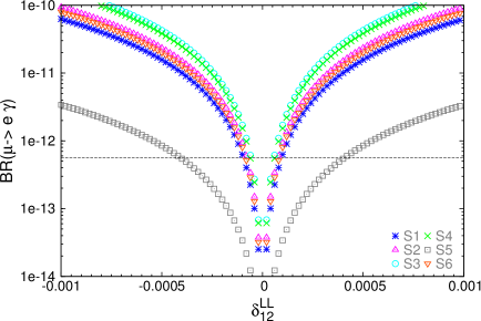
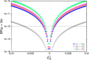
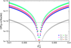
Figure 8.2: LFV rates for $\mu-e$ transitions as a function of slepton mixing $\delta_{12}^{LL}$ for scenarios S1 to S6 defined in Section 5.2.2.3. The horizontal lines are the corresponding upper bounds collected in Section 8.1.3.

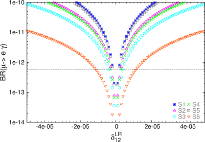
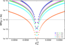
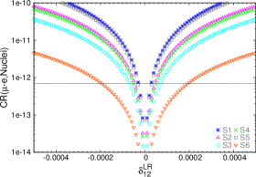
Figure 8.3: LFV rates for $\mu-e$ transitions as a function of slepton mixing $\delta_{12}^{LR}$ for scenarios S1 to S6 defined in Section 5.2.2.3. The horizontal lines are the corresponding upper bounds collected in Section 8.1.3. The corresponding plots for $\delta_{12}^{RL}$, not shown here, are indistinguishable from these.

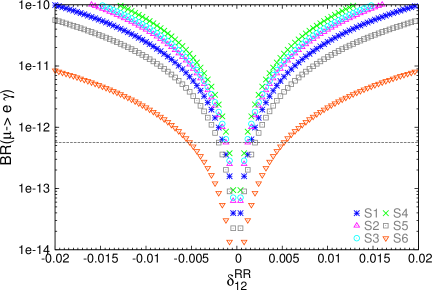
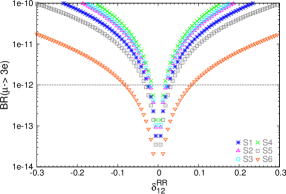
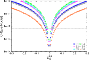
Figure 8.4: LFV rates for $\mu-e$ transitions as a function of slepton mixing $\delta_{12}^{RR}$ for scenarios S1 to S6 defined in Section 5.2.2.3. The horizontal lines are the corresponding upper bounds collected in Section 8.1.3.

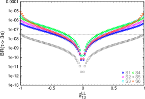
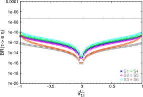
Figure 8.5: LFV rates for $\tau-e$ transitions as a function of slepton mixing $\delta_{13}^{LL}$ for scenarios S1 to S6 defined in Section 5.2.2.3. The horizontal lines are the corresponding upper bounds collected in Section 8.1.3.

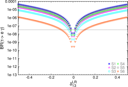
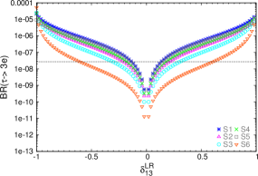
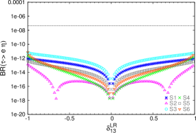
Figure 8.6: LFV rates for $\tau-e$ transitions as a function of slepton mixing $\delta_{13}^{LR}$ for scenarios S1 to S6 defined in Section 5.2.2.3. The horizontal lines are the corresponding upper bounds collected in Section 8.1.3. The corresponding plots for $\delta_{13}^{RL}$, not shown here, are indistinguishable from these.

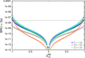
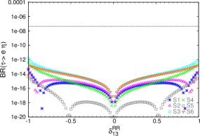
Figure 8.7: LFV rates for $\tau-e$ transitions as a function of slepton mixing $\delta_{13}^{RR}$ for scenarios S1 to S6 defined in Section 5.2.2.3. The horizontal lines are the corresponding upper bounds collected in Section 8.1.3.

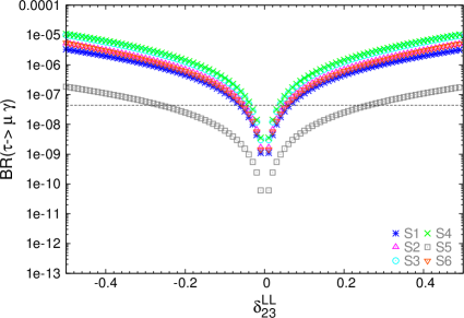
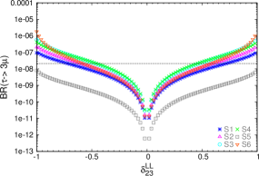
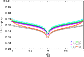
Figure 8.8: LFV rates for $\tau-\mu$ transitions as a function of slepton mixing $\delta_{23}^{LL}$ for scenarios S1 to S6 defined in Section 5.2.2.3. The horizontal lines are the corresponding upper bounds collected in Section 8.1.3.

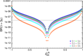
Figure 8.9: LFV rates for $\tau-\mu$ transitions as a function of slepton mixing $\delta_{23}^{LR}$ for scenarios S1 to S6 defined in Section 5.2.2.3. The horizontal lines are the corresponding upper bounds collected in Section 8.1.3. The corresponding plots for $\delta_{23}^{RL}$, not shown here, are indistinguishable from these.

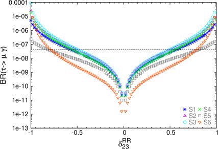
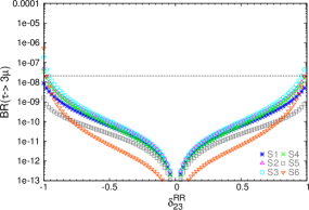
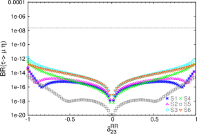
Figure 8.10: LFV rates for $\tau-\mu$ transitions as a function of slepton mixing $\delta_{23}^{RR}$ for scenarios S1 to S6 defined in Section 5.2.2.3. The horizontal lines are the corresponding upper bounds collected in Section 8.1.3.

A first look at these plots confirms the well known result that the most stringent bounds are for the mixings between the the first and the second slepton generations, 12. It is also evident that the bounds for the mixings between the second and the third slepton generations, 23, are similar to the bounds for the mixings between the first and the third generations, 13, and both are much weaker than the bounds on the 12-mixings. As another general result one can observe that, whereas all the 12-mixings are constrained by the three selected LFV processes, $\mu\to e\gamma$, $\mu\to 3e$ and $\mu-e$ conversion in heavy (Au) nuclei, the 23-mixings are not constrained, for the studied points, by the semileptonic tau decay $\tau\to\mu\eta$. Similarly, the 13-mixings are not constrained either, by $\tau\to e\eta$. The main reason for this is that the studied points S1-S6 all have very heavy $A^{0}$ Higgs bosons, $M_{A}=500-1500\,\,\mathrm{GeV}$ and therefore the decay channel mediated by this $A^{0}$ is much suppressed, even at large $\tan\beta$, where the contribution from $A^{0}$ to ${\rm BR}(\tau\to\mu\eta)$ and ${\rm BR}(\tau\to e\eta)$, which is the dominant one, grows as $(\tan\beta)^{6}$ [316, 317]. It should also be noted the appearance of two symmetric minima in ${\rm BR}(\tau\to\mu\eta)$ and ${\rm BR}(\tau\to e\eta)$ of figs 8.10 and 8.7 respectively, in the scenarios S5, S1 and S2. A similar feature can also be observed in ${\rm BR}(\tau\to e\eta)$ of fig 8.6 in scenario S2. For instance, in S5 these minima in ${\rm BR}(\tau\to e\eta)$ appear at $\delta_{13}^{RR}\sim\pm 0.5$. We have checked that the origin of these minima is due to the competing diagrams mediated by $A^{0}$ and $Z$ which give contributions of similar size for $\tan\beta\lesssim 30$ but with opposite sign, and this produces strong cancellations in the total rates. Similar comments apply to ${\rm BR}(\tau\to\mu\eta)$. Another general result, which confirms some features known in the literature for particular models like SUSY-Seesaw models [315], is the evident correlation between the ${\rm BR}(l_{j}\to 3l_{i})$ and ${\rm BR}(l_{j}\to l_{i}\gamma)$ rates. It should be emphasized that we get these correlations in a model independent way and without the use of any approximation, like the mass insertion approximation or the large $\tan\beta$ approximation. Since our computation is full-one loop and has been performed in terms of physical masses, our findings are valid for any value of $\tan\beta$ and $\delta^{AB}_{ij}$’s. These correlations, confirmed in our plots, indicate that the general prediction guided by the photon-dominance behaviour in ${\rm BR}(l_{j}\to 3l_{i})$ indeed works quite well for all the studied $\delta^{AB}_{ij}$’s and all the studied S1-S6 points. This dominance of the $\gamma$-mediated channel in the $l_{j}\to 3l_{i}$ decays allows to derive the following simplified relation:

$$\frac{{\rm BR}(l_{j}\to 3l_{i})}{{\rm BR}(l_{j}\to l_{i}\gamma)}=\frac{\alpha}{3\pi}\left(\log\frac{m_{l_{j}}^{2}}{m_{l_{i}}^{2}}-\frac{11}{4}\right)\,,$$ (8.9)

which gives the approximate values of $\frac{1}{440}$, $\frac{1}{94}$ and $\frac{1}{162}$ for $(l_{j}l_{i})=(\tau\mu),(\tau e)$ and $(\mu e)$, respectively. The ${\cal O}(\alpha)$ suppression in the predicted rates of ${\rm BR}(l_{j}\to 3l_{i})$ versus ${\rm BR}(l_{j}\to l_{i}\gamma)$ yields, despite the fact that the experimental sensitivities to the leptonic decays $l_{j}\to 3l_{i}$ have been improved considerably in the last years, that the radiative decays $l_{j}\to l_{i}\gamma$ are still the most efficient decay channels in setting constraints to the slepton mixing parameters. This holds for all the intergenerational mixings, 12, 13 and 23. As discussed in [315], in the context of SUSY, there could be just a chance of departure from these ${\cal O}(\alpha)$ reduced ratios if the Higgs-mediated channels dominate the rates of the leptonic decays, but this does not happen in our S1-S6 scenarios, with rather heavy $H^{0}$ and $A^{0}$. We have checked that the contribution from these Higgs channels are very small and can be safely neglected, a scenario that is favoured by the recent results from the heavy MSSM Higgs boson searches at the LHC [248].

This same behaviour can be seen in the comparison between the ${\rm BR}(\mu\to e\gamma)$ and ${\rm CR}(\mu-e,{\rm Nuclei})$ rates. Again there is an obvious correlation in our plots for these two rates that can be explained by the same argument as above, namely, the photon-mediated contribution in $\mu-e$ conversion dominates the other contributions, for all the studied cases, and therefore the corresponding rates are suppressed by a ${\cal O}(\alpha)$ factor respect to the radiative decay rates. These correlations are clearly seen in all our plots for all the studied $\delta^{AB}_{ij}$’s and in all S1-S6 scenarios. The relevance of ${\rm CR}(\mu-e,{\rm Nuclei})$ as compared to ${\rm BR}(\mu\to 3e)$ is given by the fact that not only the present experimental bound is slightly better, but also that the future perspectives for the expected sensitivities are clearly more promising in the $\mu-e$ conversion case (see below). In general, as can be seen in our plots, the present bounds for $\delta^{AB}_{ij}$’s as obtained from ${\rm CR}(\mu-e,{\rm Nuclei})$ and ${\rm BR}(\mu\to 3e)$ are indeed very similar.

In summary, the best bounds that one can infer from our results in figures 8.2 through 8.10 come from the radiative $l_{j}\to l_{i}\gamma$ decays and we get the maximal allowed values for all $|\delta^{AB}_{ij}|$’s that are collected in Tab. 8.1 for each of the studied scenarios S1 to S6. They give an overall idea of the size of the bounds with respect to the latest experimental data. When comparing the results in this table for the various scenarios, we see that scenario S3 gives the most stringent constraints to the $\delta^{LL}_{ij}$ and $\delta^{RR}_{ij}$ mixings, in spite of having rather heavy sleptons with masses close to 1 TeV. The reason is well understood from the $\tan\beta$ dependence of the BRs which enhances the rates in the case of $LL$ and/or $RR$ single deltas at large $\tan\beta$, in agreement with the simple results of the MIA formulas in Eqs. (8.5) and (8.6). Here it should be noted that within S3 we have $\tan\beta=50$, which is the largest considered value in these S1-S6 scenarios. Something similar happens in S4 with $\tan\beta=40$. In contrast, the most stringent constraints on the $\delta^{LR}_{ij}$ mixings occur in scenarios S1 and S5. Here it is important to note that there are not enhancing $\tan\beta$ factors in the $\delta^{LR}_{ij}$ case. In fact, the contributions from the $\delta^{LR}_{ij}$’s to the most constraining LFV radiative decay rates are $\tan\beta$ independent, in agreement again with the MIA simple expectations (see Sect. 8.1.2). Consequently, the stringent constraints on $\delta^{LR}_{i,j}$ in S1 and S5 arise due to the relatively light sleptons in these scenarios.

	S1	S2	S3	S4	S5	S6
$|\delta^{LL}_{12}|_{\rm max}$	$10\times 10^{-5}$	$7.5\times 10^{-5}$	$5\times 10^{-5}$	$6\times 10^{-5}$	$42\times 10^{-5}$	$8\times 10^{-5}$
$|\delta^{LR}_{12}|_{\rm max}$	$2\times 10^{-6}$	$3\times 10^{-6}$	$4\times 10^{-6}$	$3\times 10^{-6}$	$2\times 10^{-6}$	$1.2\times 10^{-5}$
$|\delta^{RR}_{12}|_{\rm max}$	$1.5\times 10^{-3}$	$1.2\times 10^{-3}$	$1.1\times 10^{-3}$	$1\times 10^{-3}$	$2\times 10^{-3}$	$5.2\times 10^{-3}$
$|\delta^{LL}_{13}|_{\rm max}$	$5\times 10^{-2}$	$5\times 10^{-2}$	$3\times 10^{-2}$	$3\times 10^{-2}$	$23\times 10^{-2}$	$5\times 10^{-2}$
$|\delta^{LR}_{13}|_{\rm max}$	$2\times 10^{-2}$	$3\times 10^{-2}$	$4\times 10^{-2}$	$2.5\times 10^{-2}$	$2\times 10^{-2}$	$11\times 10^{-2}$
$|\delta^{RR}_{13}|_{\rm max}$	$5.4\times 10^{-1}$	$5\times 10^{-1}$	$4.8\times 10^{-1}$	$5.3\times 10^{-1}$	$7.7\times 10^{-1}$	$7.7\times 10^{-1}$
$|\delta^{LL}_{23}|_{\rm max}$	$6\times 10^{-2}$	$6\times 10^{-2}$	$4\times 10^{-2}$	$4\times 10^{-2}$	$27\times 10^{-2}$	$6\times 10^{-2}$
$|\delta^{LR}_{23}|_{\rm max}$	$2\times 10^{-2}$	$3\times 10^{-2}$	$4\times 10^{-2}$	$3\times 10^{-2}$	$2\times 10^{-2}$	$12\times 10^{-2}$
$|\delta^{RR}_{23}|_{\rm max}$	$5.7\times 10^{-1}$	$5.2\times 10^{-1}$	$5\times 10^{-1}$	$5.6\times 10^{-1}$	$8.3\times 10^{-1}$	$8\times 10^{-1}$

Table 8.1: Present upper bounds on the slepton mixing parameters $|\delta^{AB}_{ij}|$ for the selected S1-S6 MSSM points defined in Tab. 5.2. The bounds for $|\delta^{RL}_{ij}|$ are similar to those of $|\delta^{LR}_{ij}|$.

So far, we have studied the case where just one mixing delta is allowed to be non-vanishing. However, it is known in the literature[320, 321] that one can get more stringent or more loose bounds in some particular cases if, instead, two (or even more) deltas are allowed to be non-vanishing. In order to study the implications of these scenarios with two deltas, we have analyzed the improved bounds on pairs of mixings of the 13 and 23 type which are at present the less constrained as long each delta is analyzed singly.

First we have looked into the various delta pairings of 23 type, $(\delta^{AB}_{23},\delta^{CD}_{23})$, and we have found that some of them lead to interesting interferences in the ${\rm BR}(\tau\to\mu\gamma)$ rates that can be either constructive or destructive, depending on the relative delta signs, therefore leading to either a reduction or an enhancement, respectively, in the maximum allowed delta values as compared to the one single delta case. More specifically, we have found interferences in ${\rm BR}(\tau\to\mu\gamma)$ for the case of non-vanishing $(\delta^{LR}_{23},\delta^{LL}_{23})$ pairs that are constructive if these deltas are of equal sign, and destructive if they are of opposite sign. Similarly, we have also found interferences in ${\rm BR}(\tau\to\mu\gamma)$ for the case of non-vanishing $(\delta^{RL}_{23},\delta^{RR}_{23})$ pairs that are constructive if they are of equal sign, and destructive if they are of opposite sign. However, in this latter case the size of the interference is very small and does not lead to very relevant changes with respect to the single delta case. The numerical results for the most interesting case of $(\delta^{LR}_{23},\delta^{LL}_{23})$ are shown in Fig. 8.11. We have analyzed the six previous points, S1 through S6 defined in Section 5.2.2.3, and a new point S7 with extremely heavy sleptons and whose relevant parameters for this analysis of the 23 delta bounds are as follows:

$$S7 : m_{\tilde{L}_{1,2,3}}=m_{\tilde{E}_{1,2,3}}=10000\,\,{\rm GeV}$$ (8.10)

$$\mu=2000\,\,{\rm GeV};\tan\beta=60$$

$$M_{2}=2000\,\,{\rm GeV};M_{1}=1000\,\,{\rm GeV}$$

This figure exemplifies in a clear way that for some of the studied scenarios the destructive interferences can be indeed quite relevant and produce new areas in the $(\delta^{LR}_{23},\delta^{LL}_{23})$ plane with relatively large allowed values of both $|\delta^{LR}_{23}|$ and $|\delta^{LL}_{23}|$ mixings. For instance, the orange contour which corresponds to the maximum allowed values for scenario S6, leads to allowed mixings as large as $(\delta^{LR}_{23},\delta^{LL}_{23})\sim(\pm 0.6,\mp 0.6)$. We also learn from this plot, that the relevance of this $\delta^{LR}_{23}-\delta^{LL}_{23}$ interference grows in the following order: Scenario S5 (grey contour) that has the smallest interference effect, then S1, S2, S4, S3 and S6 that has the largest interference effect. This growing interference effect is seen in the plot as the contour being rotated anti-clockwise from the most vertical one (S1) to the most inclined one (S6). Furthermore, the size of the parameter space bounded by these contours also grows, implying that “more” parameter combinations are available for these two deltas. It should be noted that, whereas the existence of the interference effect can be already expected from the simple MIA formulas of Eqs. (8.5) and (8.6), the final found shape of these contours in Fig.8.11 and their quantitative relevance cannot be explained by these simple formulas. The separation from the MIA expectations are even larger in the new studied scenario S7, as can be clearly seen in this figure. The big black contour, centred at zero, contains a rather large allowed area in the $(\delta^{LR}_{23},\delta^{LL}_{23})$ plane, allowing values, for instance, of $(\delta^{LR}_{23},\delta^{LL}_{23})\sim(\pm 0.5,\mp 0.5)$. Furthermore, in this S7 there appear new allowed regions at the upper left and lower right corners of the plot with extreme allowed values as large as $(\pm 0.9,\mp 0.9)$. These “extreme” solutions are only captured by a full one-loop calculation and cannot be explained by the simple MIA formulas.

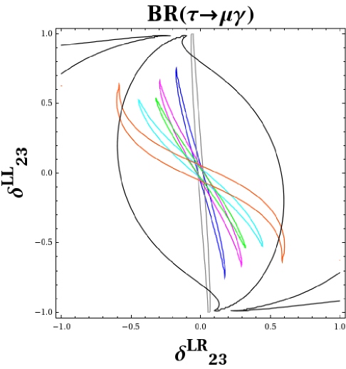
Figure 8.11: Maximum allowed values of $(\delta^{LR}_{23},\delta^{LL}_{23})$ in the scenarios S1 (dark blue), S2 (magenta), S3 (light blue), S4 (green), S5 (grey), S6 (orange) defined in Section 5.2.2.3 and S7 (black) defined in Eq. 8.10. The contourlines shown correspond to the present experimental upper limit: ${\rm BR}(\tau\to\mu\gamma)_{\rm max}=4.4\times 10^{-8}$. For each scenario the allowed deltas are those inside the corresponding contourline.

We now turn to examples in which more stringent bounds on combinations of two deltas are derived. In particular, we have explored the restrictions that are obtained on the (13,23) mixing pairs from the present bounds on ${\rm BR}(\mu\to e\gamma)$ and ${\rm CR}(\mu-e,{\rm nuclei})$. In figures 8.12 and 8.13 we show the results of this analysis for the S1 point. We have only selected the pairs where we have found improved bounds respect to the previous single delta analysis. From Fig. 8.12 we conclude that, for S1, the maximal allowed values by present $\mu\to e\gamma$ (($\mu-e$ conversion)) searches are (given specifically here for equal input deltas):

$$(|\delta^{LL}_{23}|_{\rm max},|\delta^{RL}_{13}|_{\rm max}) = (0.0015,0.0015)\,\,((0.0062,0.0062))\,\,$$ (8.11)

These numbers can be understood as follows: if, for instance, $\delta^{RL}_{13}=0.0015$ then $|\delta^{LL}_{23}|<0.0015$. If, on the other hand, one delta goes to zero the bound on the other delta disappears (from this particular observable). We find equal bounds as in Eq. (8.11) for: $(|\delta^{RL}_{23}|_{\rm max},|\delta^{LL}_{13}|_{\rm max})$, $(|\delta^{LR}_{23}|_{\rm max},|\delta^{RR}_{13}|_{\rm max})$ and $(|\delta^{RR}_{23}|_{\rm max},|\delta^{LR}_{13}|_{\rm max})$.

Other pairings of deltas give less stringent bounds than Eq. (8.11) but still more stringent than the ones from the single delta analysis. In particular, we get:

$$(|\delta^{LL}_{23}|_{\rm max},|\delta^{RR}_{13}|_{\rm max}) = (0.0073,0.0073)\,\,((0.031,0.031))\,\,$$ (8.12)

And we get equal bounds as in Eq. (8.12) for: $(|\delta^{RR}_{23}|_{\rm max},|\delta^{LL}_{13}|_{\rm max})$, $(|\delta^{LR}_{23}|_{\rm max},|\delta^{RL}_{13}|_{\rm max})$ and $(|\delta^{RL}_{23}|_{\rm max},|\delta^{LR}_{13}|_{\rm max})$.

Finally, from Fig. 8.13 we get:

$$(|\delta^{LL}_{23}|_{\rm max},|\delta^{LL}_{13}|_{\rm max}) = (0.013,0.013)\,\,((0.056,0.056))\,\,$$ (8.13)

and

$$(|\delta^{RR}_{23}|_{\rm max},|\delta^{RR}_{13}|_{\rm max}) = (0.036,0.036)\,\,((0.16,0.16))\,\,$$ (8.14)

We have also studied the implications of the future expected sensitivities in both ${\rm BR}(\mu\to e\gamma)<10^{-14}$ [329] and ${\rm CR}(\mu-e,{\rm Nuclei})<2.6\times 10^{-17}$ [330], which are anticipated from future searches. From our results in Figs. 8.12 and 8.13 we conclude that the previous bounds in Eqs. (8.11), (8.12), (8.13) and (8.14) will be improved (for both $\mu\to e\gamma$ and $\mu-e$ conversion) to $(0.0005,0.0005)$, $(0.0025,0.0025)$, $(0.005,0.005)$ and $(0.01,0.01)$, respectively.

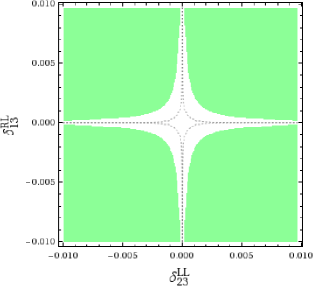
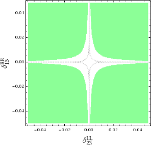
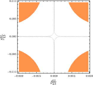
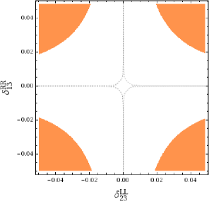
Figure 8.12: Bounds on pairs of slepton mixing parameters of (23,13) type for scenario S1: a) ($\delta_{23}^{LL}$,$\delta_{13}^{RL}$) in first column. Identical plots, not shown here, are found for: ($\delta_{23}^{RL}$,$\delta_{13}^{LL}$), ($\delta_{23}^{LR}$,$\delta_{13}^{RR}$), and ($\delta_{23}^{RR}$,$\delta_{13}^{LR}$); b) ($\delta_{23}^{LL}$,$\delta_{13}^{RR}$) in second column. Identical plots, not shown here, are found for: ($\delta_{23}^{RR}$,$\delta_{13}^{LL}$), ($\delta_{23}^{LR}$,$\delta_{13}^{RL}$), and ($\delta_{23}^{RL}$,$\delta_{13}^{LR}$). First row: Shaded regions (in green) are disallowed by the present upper experimental limit on ${\rm BR}(\mu\to e\gamma)$. Second row: Shaded regions (in orange) are disallowed by the present upper experimental limit on ${\rm CR}(\mu-e,{\rm Nuclei})$. The allowed central areas in white will be shrinked by the future expected sensitivities in both $\mu\to e\gamma$ and $\mu-e$ conversion experimental searches (see text) to the small areas around the origin delimited by the dotted lines.

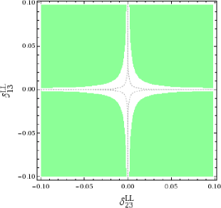
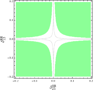
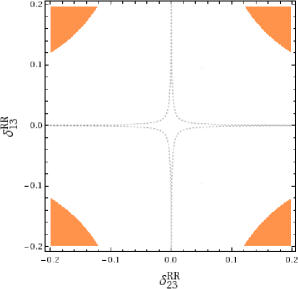
Figure 8.13: Bounds on pairs of slepton mixing parameters of (23,13) type for scenario S1: a) ($\delta_{23}^{LL}$,$\delta_{13}^{LL}$) in first column; b) ($\delta_{23}^{RR}$,$\delta_{13}^{RR}$) in second column. First row: Shaded regions (in green) are disallowed by ${\rm BR}(\mu\to e\gamma)$. Second row: Shaded regions (in orange) are disallowed by ${\rm CR}(\mu-e,{\rm Nuclei})$. All inputs and explanations are as in Fig. 8.12.

8.2.2 Numerical results for pMSSM-4 scenarios

The main goal of this part is to investigate how the upper bounds for the slepton mixing deltas that we have found previously could change for different areas of the MSSM parameter space, other than the specific selected S1-S6 points. In order to explore the variation of these bounds for different choices in the MSSM parameter space, we investigate the four qualitatively different pMSSM-4 scenarios (a), (b), (c) and (d) defined in Eqs. (5.32), (5.33), (5.34) and (5.35), respectively, in Section 5.2.2.1. As explained before, the idea is to explore generic scenarios that are compatible with present data, in particular with the measurement of a Higgs boson mass, which we interpret as the mass of the light ${\cal CP}$-even Higgs boson in the MSSM, and the present experimental measurement of $(g-2)_{\mu}$. Taking these experimental results into account, we have re-analyzed the full set of bounds for the single deltas that are extracted from the most restrictive LFV processes as a function of the two most relevant parameters in those scenarios: the generic SUSY mass scale $m_{\rm SUSY}$ $(\equiv m_{\rm SUSY-EW})$ and $\tan\beta$. In order to find $M_{h}$ around $\sim 125-126\,\,\mathrm{GeV}$ the scale $m_{\rm SUSY-QCD}$ as well as the trilinear squark couplings have been chosen to sufficiently high values, see Sect. 5.2.2.1. For the analysis in those scenarios, we use the bounds on the radiative decays, $l_{j}\to l_{i}\gamma$ which, as we have already shown, are at present the most restrictive ones in the case of one single non-vanishing delta. And to simplify the analysis in this part of the work, we use the mass insertion approximation formulas of Eqs. (8.1) through (8.4) to evaluate the ${\rm BR}(l_{j}\to l_{i}\gamma)$ rates. We have checked that these simple MIA formulas provide a sufficiently accurate estimate of the LFV rates for the present scenarios in the case of single deltas, in agreement with Ref. [321].

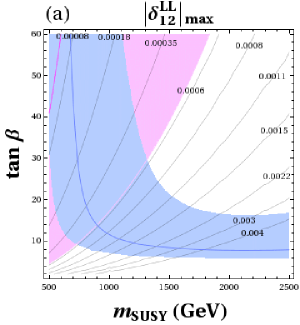
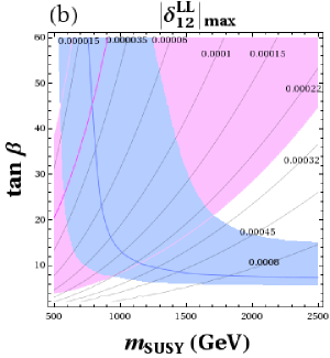
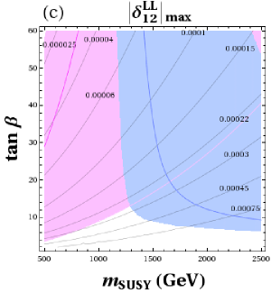
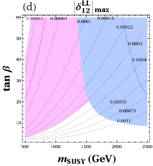
Figure 8.14: Contourlines in the ($m_{\rm SUSY}$, $\tan\beta$) plane of maximum slepton mixing $|\delta_{12}^{LL}|_{\rm max}$ that are allowed by LFV searches in $\mu\to e\gamma$ for scenarios (a), (b), (c) and (d) of the pMSSM-4 type, defined in Section 5.2.2.1. The shaded areas in pink are the regions leading to a $(g-2)_{\mu}^{\rm SUSY}$ prediction in the $(3.2,57.2)\times 10^{-10}$ interval. The interior pink contourline (without number) corresponds to setting $(g-2)_{\mu}^{\rm SUSY}$ exactly at the central value of the discrepancy $(g-2)_{\mu}^{\rm exp}-(g-2)_{\mu}^{\rm SM}=30.2\times 10^{-10}$ . The shaded overimposed areas in blue are the regions leading to a $M_{h}$ prediction within the $(123,127)\,\,\mathrm{GeV}$ interval. The interior blue contourline (without number) corresponds to the particular $M_{h}=125\,\,\mathrm{GeV}$ value.

We present the numerical results of our analysis in the pMSSM-4 scenarios that are shown in Figs. 8.14 through 8.19. Figures 8.14, 8.15 and 8.16 show the bounds for the slepton mixing of 12-type as extracted from present $\mu\to e\gamma$ searches. Figures 8.17, 8.18 and 8.19 show the bounds for the slepton mixing of 23-type as extracted from present $\tau\to\mu\gamma$ searches. It should be noted that the bounds for the slepton mixings of 13-type (not shown here) are equal (in the MIA) to those of 23-type. In each plot we show the resulting contourlines in the ($m_{\rm SUSY}$, $\tan\beta$) plane of maximum allowed slepton mixing. In addition we also show in each plot the areas in the pMSSM-4 parameter space for that particular scenario that lead to values of the lightest Higgs boson mass compatible with LHC data, and at the same time to predictions of the muon anomalous magnetic moment also compatible with data. As in the set of pMSSM points of the previous section, we use here again FeynHiggs [238, 239, 240, 103] to evaluate $M_{h}$ and SPHENO [237] to evaluate $(g-2)_{\mu}$ (where FeynHiggs gives very similar results). The shaded areas in pink are the regions leading to a $(g-2)_{\mu}^{\rm SUSY}$ prediction, from the SUSY one-loop contributions, in the allowed by data $(3.2,57.2)\times 10^{-10}$ interval. The interior pink contourline corresponds to setting $(g-2)_{\mu}^{\rm SUSY}$ exactly at the central value of the discrepancy $(g-2)_{\mu}^{\rm exp}-(g-2)_{\mu}^{\rm SM}=30.2\times 10^{-10}$. The shaded overimposed areas in blue are the regions leading to a $M_{h}$ prediction within the $(123,127)\,\,\mathrm{GeV}$ interval. The interior blue contourline corresponds to the particular $M_{h}=125\,\,\mathrm{GeV}$ value.

From these plots in the ($m_{\rm SUSY}$, $\tan\beta$) plane one can draw the following conclusions:

• For each scenario (a), (b), (c) and (d) one can derive the corresponding upper bound for each $|\delta^{AB}_{ij}|$ at a given ($m_{\rm SUSY}$, $\tan\beta$) point in this plane.

• The maximal allowed values of the $\delta^{LL}_{ij}$’s and $\delta^{RR}_{ij}$’s scale with $m_{\rm SUSY}$ and $\tan\beta$ approximately as expected, growing with increasing $m_{\rm SUSY}$ as $\sim m_{\rm SUSY}^{2}$ and decreasing with increasing (large) $\tan\beta$ as $\sim 1/\tan\beta$. The maximal allowed values of the $\delta^{LR}_{ij}$’s (and similarly $\delta^{RL}_{ij}$’s) are independent on $\tan\beta$ and grow approximately as $\sim m_{\rm SUSY}$ with increasing $m_{\rm SUSY}$. This is in agreement with the qualitative behaviour found in the approximation formulas, Eqs. (8.5) and (8.6) of the MIA results in the simplest case of only one mass scale, $m_{S}$.

• The intersections between the allowed areas by the required $(g-2)_{\mu}$ and $M_{h}$ intervals move from the left side, $m_{\rm SUSY}\sim 500-1300\,\,\mathrm{GeV}$ to the right side of the plots, $m_{\rm SUSY}\sim 1300-2500\,\,\mathrm{GeV}$ from scenarios (a) through (d). This is clearly the consequence of the fact that $(g-2)_{\mu}$ requires a rather light SUSY-EW sector, i.e. light charginos, neutralinos and sleptons, and a rather large $\tan\beta$, and that $M_{h}$ requires a rather heavy SUSY squark sector. Remember that here we are using a common reference SUSY scale $m_{\rm SUSY}$, relating all the SUSY sparticle masses, both in the SUSY-EW and SUSY-QCD sectors, leading to this “tension”. (A more loose connection between these two sectors would yield a more relaxed combination of the $(g-2)_{\mu}$ and $M_{h}$ experimental results.) In fact, in our plots one can observe that the particular contourlines for the “preferred” values of $(g-2)_{\mu}$ and $M_{h}$ by data (i.e. the interior blue and pink contourlines) only cross in scenario (b) at $m_{\rm SUSY}$ around $800\,\,\mathrm{GeV}$ and $\tan\beta\sim 45$ and get close, although not crossing, in scenario (a) at $m_{\rm SUSY}\sim 650\,\,\mathrm{GeV}$ and very large $\tan\beta\sim 60$. However, taking the uncertainties into account the overlap regions are quite substantial.

• By assuming a favoured region in the ($m_{\rm SUSY}$,$\tan\beta$) parameter space given by the intersect of the two $(g-2)_{\mu}$ (in pink) and $M_{h}$ (in blue) areas, one can extract improved bounds for the slepton mixing deltas valid in these intersects. Those bounds give a rough idea of which parameter regions in the pMSSM-4 are in better agreement with the experimental data on $(g-2)_{\mu}$ and $M_{h}$. The following intervals for the maximum allowed $|\delta^{AB}_{ij}|$ values can be deduced from our plots in these intersecting regions:

  Scenario (a):

  $|\delta^{LL}_{12}|_{\rm max}\sim(6,60)\times 10^{-5}$

  $|\delta^{LR}_{12}|_{\rm max}\sim(1.2,3.2)\times 10^{-6}$

  $|\delta^{RR}_{12}|_{\rm max}\sim(3,25)\times 10^{-3}$

  $|\delta^{LL}_{23}|_{\rm max}\sim(3,35)\times 10^{-2}$

  $|\delta^{LR}_{23}|_{\rm max}\sim(1,3.2)\times 10^{-2}$

  $|\delta^{RR}_{23}|_{\rm max}\sim(10)\times 10^{-1}$

  Scenario (b):

  $|\delta^{LL}_{12}|_{\rm max}\sim(1.5,27)\times 10^{-5}$

  $|\delta^{LR}_{12}|_{\rm max}\sim(3,9.2)\times 10^{-6}$

  $|\delta^{RR}_{12}|_{\rm max}\sim(0.35,7)\times 10^{-3}$

  $|\delta^{LL}_{23}|_{\rm max}\sim(0.7,15)\times 10^{-2}$

  $|\delta^{LR}_{23}|_{\rm max}\sim(3,9.5)\times 10^{-2}$

  $|\delta^{RR}_{23}|_{\rm max}\sim(2,10)\times 10^{-1}$

  Scenario (c):

  $|\delta^{LL}_{12}|_{\rm max}\sim(5,22)\times 10^{-5}$

  $|\delta^{LR}_{12}|_{\rm max}\sim(5,22)\times 10^{-6}$

  $|\delta^{RR}_{12}|_{\rm max}\sim(1.2,10)\times 10^{-3}$

  $|\delta^{LL}_{23}|_{\rm max}\sim(3,15)\times 10^{-2}$

  $|\delta^{LR}_{23}|_{\rm max}\sim(5,22)\times 10^{-2}$

  $|\delta^{RR}_{23}|_{\rm max}\sim(6,10)\times 10^{-1}$

  Scenario (d):

  $|\delta^{LL}_{12}|_{\rm max}\sim(10,30)\times 10^{-5}$

  $|\delta^{LR}_{12}|_{\rm max}\sim(5,9)\times 10^{-6}$

  $|\delta^{RR}_{12}|_{\rm max}\sim(1.2,4)\times 10^{-3}$

  $|\delta^{LL}_{23}|_{\rm max}\sim(5,20)\times 10^{-2}$

  $|\delta^{LR}_{23}|_{\rm max}\sim(5,9.5)\times 10^{-2}$

  $|\delta^{RR}_{23}|_{\rm max}\sim(7,10)\times 10^{-1}$

It should be noted that in the previous upper bounds, the particular $10\times 10^{-1}$ value appearing in $|\delta^{RR}_{23}|_{\rm max}$ really means 1 or larger that 1, since we have not explored out of the $-1\leq\delta^{AB}_{ij}\leq 1$ intervals. Particularly, in scenario (a) which has the heaviest gauginos, we find that all values in the $-1\leq\delta^{RR}_{23}\leq 1$ interval are allowed by LFV data.

Finally, one can shortly summarize the previous $|\delta^{AB}_{ij}|_{\rm max}$ intervals found from LFV searches, by just signalling the typical intervals for each delta, in the favoured by LHC and $(g-2)_{\mu}$ data MSSM parameter space region, where the predictions in all scenarios lay at: $|\delta^{LL}_{12}|_{\rm max}\sim{\cal O}(10^{-5},10^{-4})$, $|\delta^{LR}_{12}|_{\rm max}\sim{\cal O}(10^{-6},10^{-5})$, $|\delta^{RR}_{12}|_{\rm max}\sim{\cal O}(10^{-3},10^{-2})$, $|\delta^{LL}_{23}|_{\rm max}\sim{\cal O}(10^{-2},10^{-1})$, $|\delta^{LR}_{23}|_{\rm max}\sim{\cal O}(10^{-2},10^{-1})$, $|\delta^{RR}_{23}|_{\rm max}\sim{\cal O}(10^{-1},10^{0})$. Very similar general bounds as for the 23 mixing are found for the 13 mixing.

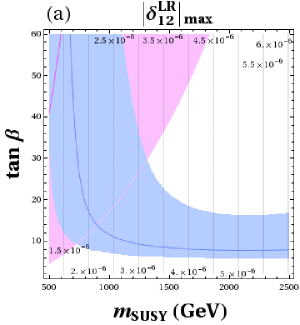
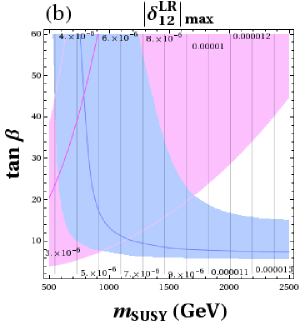
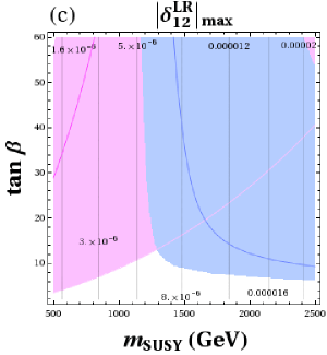
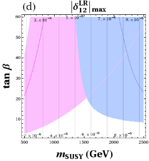
Figure 8.15: Contourlines in the ($m_{\rm SUSY}$, $\tan\beta$) plane of maximum slepton mixing $|\delta_{12}^{LR}|_{\rm max}$ that are allowed by LFV searches in $\mu\to e\gamma$. All inputs and explanations are as in Fig. 8.14.

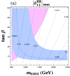
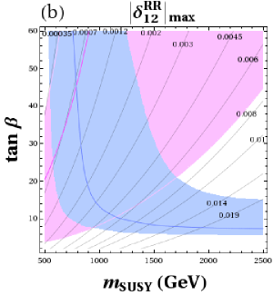
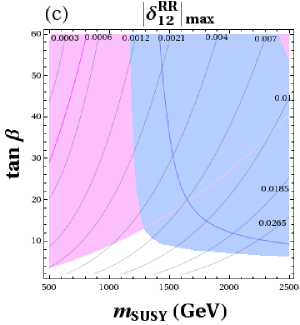
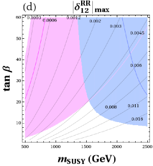
Figure 8.16: Contourlines in the ($m_{\rm SUSY}$, $\tan\beta$) plane of maximum slepton mixing $|\delta_{12}^{RR}|_{\rm max}$ that are allowed by LFV searches in $\mu\to e\gamma$. All inputs and explanations are as in Fig. 8.14.

Figure 8.17: Contourlines in the ($m_{\rm SUSY}$, $\tan\beta$) plane of maximum slepton mixing $|\delta_{23}^{LL}|_{\rm max}$ that are allowed by LFV searches in $\tau\to\mu\gamma$. All inputs and explanations are as in Fig. 8.14. Similar results/plots (not shown) are obtained for contourlines of maximum slepton mixing $|\delta_{13}^{LL}|_{\rm max}$ that are allowed by LFV searches in $\tau\to e\gamma$.

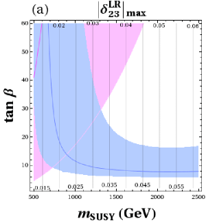
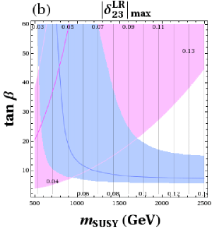
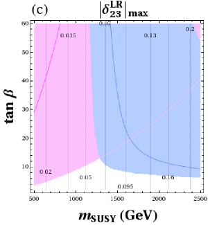
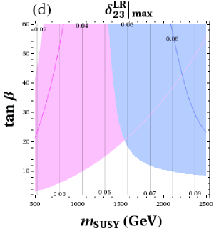
Figure 8.18: Contourlines in the ($m_{\rm SUSY}$, $\tan\beta$) plane of maximum slepton mixing $|\delta_{23}^{LR}|_{\rm max}$ that are allowed by LFV searches in $\tau\to\mu\gamma$. All inputs and explanations are as in Fig. 8.14. Similar results/plots (not shown) are obtained for contourlines of maximum slepton mixing $|\delta_{13}^{LR}|_{\rm max}$ that are allowed by LFV searches in $\tau\to e\gamma$.

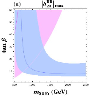
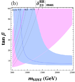
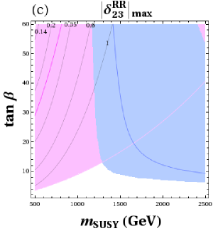
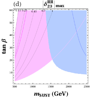
Figure 8.19: Contourlines in the ($m_{\rm SUSY}$, $\tan\beta$) plane of maximum slepton mixing $|\delta_{23}^{RR}|_{\rm max}$ that are allowed by LFV searches in $\tau\to\mu\gamma$. All inputs and explanations are as in Fig. 8.14. Notice that only contourlines with $|\delta_{23}^{RR}|_{\rm max}\leq 1$ are included. In the scenario (a) the countourlines with $|\delta_{23}^{RR}|_{\rm max}\leq 1$ are out of the region in the parameter space shown in this figure. Similar results/plots (not shown) are obtained for contourlines of maximum slepton mixing $|\delta_{13}^{RR}|_{\rm max}$ that are allowed by LFV searches in $\tau\to e\gamma$.

Chapter 9 LFV Higgs decays from flavour mixing in the slepton sector

In this chapter we complete our study of LFV processes with a research on some interesting LFV Higgs decays which will happen in presence of flavour mixing in the slepton sector. The detection of these decays in the LHC would be a clear signal of new physics beyond the SM, and as we will see through this chapter, these decays will provide a unique window to the MSSM even for a very heavy SUSY spectrum.

The results in this chapter have been published in [74].

9.1 Motivation for the study of LFV Higgs decays

The absence of any experimental signal, so far, in the searches for supersymmetry at the LHC [331] and the discovery of a new Higgs-like particle by ATLAS [4] and CMS [5], are pushing some SUSY mass parameters above the 1-TeV range. On one hand, the present lower mass bounds for squarks of the first and second generations and for gluinos are already above 1 TeV, and on the other hand, if the observed Higgs boson is identified with the lightest Higgs boson $h$ of the Minimal Supersymmetric Standard Model, a radiatively corrected mass $m_{h}\simeq$ 125-126 GeV also suggests that some third generation squarks could be in the TeV range. In principle, to place the SUSY masses at the multi-TeV range seems discouraging, both from an experimental point of view due to the inability to detect SUSY directly, and from a theoretical point of view, in regard to the naturalness of the theory, which contrarily suggests a soft SUSY-breaking scale, $m_{\rm SUSY}$, at or below the TeV scale. However, leaving the naturalness issue aside, the MSSM scenarios with very heavy SUSY masses can have other interesting aspects [332]. In particular, this is the case of specific Higgs boson observables, like certain Higgs partial decay widths, which present a non-decoupling behaviour with $m_{\rm SUSY}$, as shown, for instance, in [333, 334, 303, 304, 57], opening a new window to the indirect detection of heavy SUSY. As it is well known, the decoupling of SUSY radiative corrections in the asymptotic large SUSY mass limit is valid for SUSY theories with an exact gauge symmetry, in agreement with the general decoupling behaviour of heavy states in Quantum Field Theory as stated in the famous Appelquist-Carazzone theorem [335]. Nevertheless, it is also known that this theorem does not apply to theories with spontaneously broken gauge symmetries, nor with chiral fermions, which is the case of the MSSM. Furthermore, in order to have decoupling, the dimensionless couplings should not grow with the heavy masses. Otherwise, the mass suppression induced by the heavy-particle propagators can be compensated by the mass enhancement provided by the interaction vertices, with an overall non-decoupling effect, which is exactly what happens in some MSSM Higgs boson decays to fermions. For instance, it was studied in [333] how non decoupling appears for large SUSY masses in the $h\to b\bar{b}$ decay through one-loop SUSY-QCD corrections, when the involved SUSY particle masses grow simultaneously with a generic soft SUSY-breaking scale $m_{\rm SUSY}$ (see also [334]). A similar non-decoupling behaviour was obtained for flavour changing neutral Higgs boson decays into quarks of the second and third generations through both SUSY-QCD corrections [303] and SUSY-EW corrections [304]. Other interesting non-decoupling SUSY-EW effects have also been seen in lepton flavour violating (LFV) Higgs boson decays within the context of the MSSM-seesaw model [57]; and in Higgs-mediated LFV processes like: $\tau\to 3\mu$ decays [315], some semileptonic $\tau$ decays [316, 317] and in $\mu-e$ conversion in heavy nuclei [318]; all of them within the MSSM-seesaw model too. Other non-decoupling effects from heavy SUSY particles have also been noticed within the context of the SUSY inverse-seesaw model [336]. Some studies of SUSY non decoupling within the MSSM have also been performed in the effective field theory approach where the effective Higgs-fermion-fermion vertices are induced from one-loop corrections of heavy SUSY particles [334, 235, 322] and in $b\bar{b}h$ production [337].

In the present chapter, motivated by the recent discovery of the SM-like Higgs boson, we will focus on the study of the LFV Higgs boson decays at one-loop order with the hypothesis of general slepton flavour mixing. We will extend the study to the three neutral Higgs bosons of the MSSM $h$, $H$ and $A$, considering the new Higgs-like particle to be the lightest Higgs boson $h$. In particular, we will study the LFV Higgs decays $h\to\tau\mu$, $H\to\tau\mu$ and $A\to\tau\mu$. This kind of processes provide an unique window into new physics due to the strong suppression of flavour violation in the SM, where the flavour mixing is induced exclusively by the Yukawa couplings of the corresponding fermion sector. This is specially interesting in the lepton sector in which the flavour mixing will be hugely suppressed because of the smallness of the lepton Yukawa couplings. Therefore, the discovery of any process which violates the lepton flavour number would be a clear signal of physics beyond the SM. The specific case of LFV Higgs decays within supersymmetric models has deserved special attention in the literature [57, 338]. Also encouraging results for the reach of LFV Higgs decays at the LHC have been recently obtained in [339] within the context of a general effective Lagrangian approach.

Our purpose here is to take advantage of the mentioned non-decoupling behaviour with $m_{\text{SUSY}}$ in the LFV Higgs decay widths into charged leptons of different generations, $\Gamma(\phi\to l_{i}l_{j})$, with $i\neq j$ and $\phi=h,H,A$, in order to look for sizeable branching ratios which can give rise to detectable signals at the LHC. Here and from now on, $l_{i}l_{j}$ with $i\neq j$ in the final state of the LFV decays refers to either $l_{i}{\bar{l}}_{j}$ or ${\bar{l}}_{i}l_{j}$. In general, the radiatively corrected LFV Higgs couplings to leptons are proportional to the heaviest lepton mass involved, being this the reason why we select the $\tau\mu$ channel as the most promising one. In addition, the $\mu e$ channel is extremely restricted by the associated radiative decay, $\mu\to e\gamma$ [225], leaving us almost no room to move in the allowed parameter space of slepton flavour mixing, and driving us to extremely low rates, not measurable in any LHC detector. The $\tau e$ channel, on the other hand, gives us very similar results to the $\tau\mu$ channel, and from an experimental point of view, the LHC sensitivity to the former should be equivalent to the latter [340]. Therefore the results obtained along this chapter for the LFV Higgs decays into $\tau\mu$ are straightforwardly translated into the $\tau e$ channels. For the present study we will focus then on the $\phi\to\tau\mu$ decays within the MSSM at one loop with general slepton flavour mixing between the second and the third generations, without assuming any particular source of flavour mixing.

The general slepton mixing will be parametrized in a model-independent way as it was explained in Section 5.1.2. As we learned from Chapter 8, when we studied the constraints to the flavour mixing parameters, the most important constraints to the four slepton mixings that we will study here come from the $\tau\to\mu\gamma$ searches [212]. The present bounds obtained there to BR$(\tau\to\mu\gamma)$ lead to constraints on the 23 mixings which for 500 GeV $\leq\,m_{\rm SUSY}\,\leq$ 1500 GeV and 5 $\leq\,\tan\beta\,\leq$ 60 are at $|\delta^{LL}_{23}|_{\rm max},|\delta^{LR}_{23}|_{\rm max},|\delta^{RL}_{23}|_{\rm max}\sim{\cal O}(10^{-2}-10^{-1})$, and $|\delta^{RR}_{23}|_{\rm max}\sim{\cal O}(10^{-1}-1)$, and for heavier SUSY masses lead to weaker bounds. We will check here, that by raising the SUSY mass scale into the multi-TeV range will turn into the needed relaxation of these bounds, since these LFV radiative decays present a decoupling behaviour with the SUSY scale. This will allow us to explore a high SUSY mass scale region, where we will find very promising values for the LFV Higgs rates.

9.2 Framework for the computation of the LFV decay rates BR$(\phi\to l_{i}l_{j})$

For the forthcoming estimates of the LFV Higgs decay rates, we use the complete one-loop formulas and the full set of diagrams contributing to the $\Gamma(\phi\to{\bar{l}_{i}}l_{j})$ and $\Gamma(\phi\to l_{i}{\bar{l}_{j}})$ partial decay widths, with $i\neq j$, within the MSSM, which are written in terms of the mass eigenvalues for all the involved MSSM sparticles, including the physical slepton and sneutrino masses, $m_{\tilde{l}_{i}}\,\,(i=1,..,6)$ and $m_{\tilde{\nu}_{i}}\,\,(i=1,2,3)$, and the rotation matrices $R^{\tilde{l}}$ and $R^{\tilde{\nu}}$ of Eqs. (5.27) and  (5.28). We take these general one-loop formulas from [57] and emphasize that they are valid for the general slepton mixing case considered here, with all the mixings effects from the $\delta^{AB}_{ij}$’s being transmitted to the LFV Higgs decay rates via the physical slepton and sneutrino masses and their corresponding rotations. The off-diagonal trilinear couplings in Eq.(5.23) also enter into this computation of the LFV Higgs decay rates. For a more detailed discussion about these analytical results we refer the reader to [57]. It should be also noted that, since we are assuming real $\delta^{AB}_{ij}$’s, the predictions for BR$(\phi\to l_{i}{\bar{l}_{j}})$ and the ${\cal CP}$-conjugate BR$(\phi\to{\bar{l}_{i}}l_{j})$ are the same. Thus, we will perform our estimates for just one of them and will denote this rate generically by BR$(\phi\to l_{i}l_{j})$. Obviously, in the case that these two channels cannot be differentiated experimentally one should then add the two contributions to the total final number of events. However, for the present computation we do not sum them and report instead the results for $\phi\to l_{i}l_{j}$, meaning that they are valid for any of the two cases.

As said above, we focus only on $h\to\tau\mu$, $H\to\tau\mu$ and $A\to\tau\mu$ decay channels and consider the constraints imposed over the parameter space by the current upper bound on the related LFV radiative decay $\tau\to\mu\gamma$ [212]. The SUSY mass spectra are computed numerically with the code SPheno [237]. The slepton and sneutrino spectra are computed from an additional subroutine that we have implemented into SPheno in order to include our parametrization of slepton mixing given by the $\delta^{AB}_{ij}$’s. The LFV decay rates are computed with our private FORTRAN code in which we have implemented the complete one-loop formulas for the LFV partial Higgs decay widths of [57] and the complete one-loop formulas for the LFV radiative $\tau$ decay widths which we take from [315]. Note that these latter formulas for the $\tau\to\mu\gamma$ decays are also written in terms of the physical sparticle eigenvalues and eigenstates and do not neglect any of the lepton masses. The mass spectrum of the MSSM Higgs sector, with two-loop corrections included, and their corresponding total widths are calculated by means of the code FeynHiggs [238] as in the previous chapters.

In the numerical computations of this study of the Higgs decays we will work within the scenarios defined in Section 5.2 and we will restrict ourselves to the case where there are flavour mixings exclusively between the second and third generations of sleptons, thus we set all $\delta_{ij}^{AB}$’s to zero except for $ij=23$. On one hand, the LFV one-loop corrected Higgs couplings are proportional to the heaviest lepton mass involved [57] and, therefore, the Higgs decay rates into $\mu e$ are suppressed by a factor $m_{\mu}^{2}/m_{\tau}^{2}$ with respect to the $h,H,A\to\tau\mu,\tau e$ decay rates. On the other hand, the related LFV radiative decay $\mu\to e\gamma$ has a much more restrictive upper bound [225] than $\tau\to e\gamma$ and $\tau\to\mu\gamma$ decays [212], and the present allowed values of the $\delta_{12}^{AB}$’s would not drive us to any measurable $\phi\to\mu e$ rates.

9.3 Numerical results for the branching ratios of the LFV decays

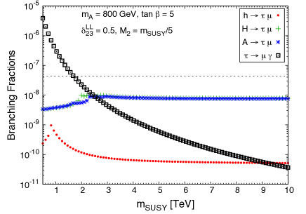
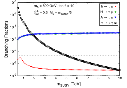
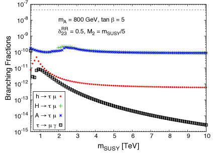
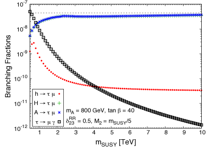
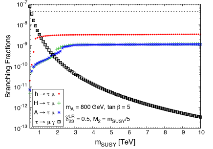
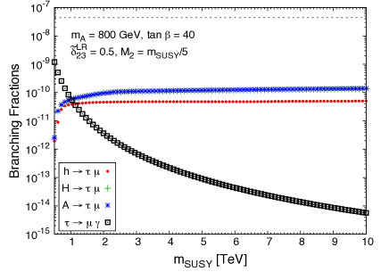
Figure 9.1: Large $m_{\text{SUSY}}$ behaviour of the LFV decay rates for the scenarios defined in Section 5.2.2.2: BR($h\to\tau\mu$), BR($H\to\tau\mu$), BR($A\to\tau\mu$) and BR($\tau\to\mu\gamma$) as functions of $m_{\text{SUSY}}$ for $\tan\beta=5$ (left panels) and $\tan\beta=40$ (right panels) with $\delta_{23}^{LL}=0.5$ (upper panels), $\delta_{23}^{RR}=0.5$ (middle panels) and $\tilde{\delta}_{23}^{LR}=0.5$ (lower panels). The results for $\tilde{\delta}_{23}^{RL}=0.5$ (not shown) are identical to those of $\tilde{\delta}_{23}^{LR}=0.5$. In each case, the other flavour changing deltas are set to zero. In all panels, $m_{A}=$ 800 GeV and the other MSSM parameters are set to the values reported in the text, with $M_{2}=\frac{1}{5}m_{\text{SUSY}}$. The horizontal dashed line denotes the current experimental upper bound for $\tau\to\mu\gamma$ channel, BR($\tau\to\mu\gamma$) $<4.4\times 10^{-8}$ [212].

Next we present the numerical results for the branching ratios of the LFV decays. The scenarios that will be evaluated are described in Section 5.2.2.2, with a detailed discussion of the possible values of the parameters.

We recall that in these scenarios the relevant mass parameters are:

$$m_{\tilde{L}} = m_{\tilde{E}}=m_{\text{SUSY}}\,,$$ (9.1)

$$\mu = M_{2}=a\,m_{\text{SUSY}}\,,$$ (9.2)

where $a$ is a constant coefficient that we will fix to different values, namely, $a=\frac{1}{5}$, $\frac{1}{3}$, 1.

We also set an approximate GUT inspired relation for the gaugino masses:

$$M_{2}=2M_{1}=M_{3}/4\,.$$ (9.3)

And the trilinear couplings in the slepton sector have been fixed to the generic SUSY mass scale, $A_{\mu}=A_{e}=A_{\tau}=m_{\text{SUSY}}$.

Regarding the non-diagonal trilinear couplings in the slepton sector we have also assumed a rather simple but realistic setting by relating them with the single soft SUSY-breaking mass scale, $m_{\text{SUSY}}$. Specifically, we assume the following linear relation:

$${\cal A}^{l}_{23} = {\tilde{\delta}}^{LR}_{23}m_{\text{SUSY}}\,,\,\,\,\,\,{\cal A}^{l}_{32}={\tilde{\delta}}^{LR}_{32}m_{\text{SUSY}}\,.$$ (9.4)

We show in Figure 9.1 the behaviour of the branching ratios for the two types of LFV decays, BR$(\phi\to\tau\mu)$ and BR$(\tau\to\mu\gamma$), as functions of $m_{\text{SUSY}}$, and we consider two different values of $\tan\beta$, namely, $\tan\beta=5$ (left panels) and $\tan\beta=40$ (right panels). In each case we set one single delta to be non vanishing with the particular values: $\delta_{23}^{LL}=0.5$ (upper panels), $\delta_{23}^{RR}=0.5$ (middle panels) and ${\tilde{\delta}}_{23}^{LR}=0.5$ (lower panels). All the other flavour changing deltas are set to zero. We find identical results for ${\tilde{\delta}}_{23}^{RL}=0.5$ as for ${\tilde{\delta}}_{23}^{LR}=0.5$ and, for brevity, we have omitted the plots for ${\tilde{\delta}}_{23}^{RL}$ in Figure 9.1.

On the upper panels of Figure 9.1, when the responsible for the flavour mixing between the second and the third generations is $\delta_{23}^{LL}$, the branching ratios of the LFV Higgs decays show a clear non-decoupling behaviour with $m_{\text{SUSY}}$, which remain constant from $m_{\text{SUSY}}\simeq$ 1 TeV to $m_{\text{SUSY}}=$ 10 TeV, with values of BR$(h\to\tau\mu)\simeq 5\times 10^{-11}$ and BR$(H,A\to\tau\mu)\simeq 8\times 10^{-9}$ for $\tan\beta=$ 5, and BR$(h\to\tau\mu)\simeq 3\times 10^{-9}$ and BR$(H,A\to\tau\mu)\simeq 3\times 10^{-6}$ for $\tan\beta=$ 40. Another important feature that should be noted is the fast growing with $\tan\beta$ of these decays which increase the $H$ and $A$ LFV decay rates almost three orders of magnitude from $\tan\beta=$ 5 to $\tan\beta=$ 40. Furthermore, we have numerically checked that for large values of $\tan\beta\geq 10$ the partial decay widths $\Gamma(H,A\to\tau\mu)$ go approximately as $\sim(\tan\beta)^{4}$ [57], whereas $\Gamma(h\to\tau\mu)$ goes as $\sim(\tan\beta)^{2}$. This implies that the corresponding branching ratios go all at large $\tan\beta\geq 10$ as BR($h,H,A\to\tau\mu$) $\sim(\tan\beta)^{2}$ in this $LL$ case, since the total widths go as $\Gamma_{\text{tot}}(H,A)\sim(\tan\beta)^{2}$ and $\Gamma_{\text{tot}}(h)$ is approximately constant with $\tan\beta$. This behaviour of the BRs with $\tan\beta$ is confirmed numerically in our forthcoming Figure 9.2. In contrast, the branching ratio of the $\tau\to\mu\gamma$ decay presents a decoupling behaviour with $m_{\text{SUSY}}$, decreasing as $\sim 1/m_{\text{SUSY}}^{4}$, and it is reduced around five orders of magnitude from $m_{\text{SUSY}}=$ 500 GeV to $m_{\text{SUSY}}=$ 10 TeV. In all these figures we have also included, for comparison, the experimental upper bound for the $\tau\to\mu\gamma$ channel, whose present value is BR($\tau\to\mu\gamma$) $<4.4\times 10^{-8}$ [212]. Thus, each $m_{\text{SUSY}}$ point which leads to a prediction of BR$(\tau\to\mu\gamma)$ above this line is excluded by data. Therefore, only values of $m_{\text{SUSY}}\gtrsim$ 2 TeV for $\tan\beta=$ 5 and $m_{\text{SUSY}}\gtrsim$ 5 TeV for $\tan\beta=$ 40, and their corresponding predictions for the LFV rates, are allowed for $\delta_{23}^{LL}=0.5$.

On the middle panels of Figure 9.1 we have plotted the LFV Higgs and radiative decay rates as functions of $m_{\text{SUSY}}$, considering $\delta_{23}^{RR}$ as the responsible for $\tau-\mu$ mixing. A similar non-decoupling behaviour to the $\delta_{23}^{LL}$ case can be observed for $\delta_{23}^{RR}$, whose branching ratios stay again constant as $m_{\text{SUSY}}$ grows. However, the numerical contribution of $\delta_{23}^{RR}$ to the LFV processes is much less important than that of $\delta_{23}^{LL}$, and all the $RR$ rates are in comparison around two orders of magnitude smaller than the $LL$ rates. In the $RR$ case, another important feature is that all the predictions found of BR($\tau\to\mu\gamma$) for $5\leq\tan\beta\leq 40$ and $m_{\text{SUSY}}$ values above 500 GeV are allowed by the present BR$(\tau\to\mu\gamma)$ experimental upper bound.

The predictions of BR($h\to\tau\mu$), BR($H\to\tau\mu$), BR($A\to\tau\mu$) and BR($\tau\to\mu\gamma$) as functions of $m_{\text{SUSY}}$, for the case ${\tilde{\delta}}_{23}^{LR}=$ 0.5, are shown on the lower panels of Figure 9.1. We see clearly again a non-decoupling behaviour with $m_{\text{SUSY}}$, since the branching ratios of the Higgs decays tend to a constant value as $m_{\text{SUSY}}$ grows, in contrast to the BR$(\tau\to\mu\gamma)$ rates that display again a decoupling behaviour and decrease with $m_{\text{SUSY}}$. For this particular choice of ${\tilde{\delta}}_{23}^{LR}=$ 0.5 we also see that the predicted branching ratios for the LFV $h$ decays at low $\tan\beta=5$ are larger than in the previous $LL$ and $RR$ cases, whereas the branching ratios for the LFV $H$ and $A$ decays are larger than those of the $RR$ case but smaller than the $LL$ ones. The lower right panel shows that for $\tan\beta=40$ the branching ratios of the three Higgs bosons, $h$, $H$ and $A$, are comparatively smaller than for $\tan\beta=5$. This decreasing with $\tan\beta$ of the LFV decay rates for the $LR$ case with fixed value of ${\tilde{\delta}}_{23}^{LR}$ is confirmed in our forthcoming Figure 9.2. In consequence, the largest LFV Higgs decay rates that will be obtained in the $LR$ (and $RL$) case will be for low $\tan\beta$ values and this will be taken into account in our next studies in order to maximize the event rates from these decays at the LHC.

To sum up the main results of Figure 9.1, the most relevant $\delta_{23}^{AB}$ parameter at low $\tan\beta$ values for the lightest Higgs boson $h$ is ${\tilde{\delta}}_{23}^{LR}$ (and ${\tilde{\delta}}_{23}^{RL}$), which gives rise to larger LFV Higgs decay rates than $\delta_{23}^{LL}$ and $\delta_{23}^{RR}$, whereas for the $H$ and $A$ Higgs bosons the most relevant parameter is $\delta_{23}^{LL}$. At large $\tan\beta$ values, the most relevant parameter for all the three Higgs bosons is $\delta_{23}^{LL}$. All these branching ratios, as we will see later, can be further enhanced by considering two non-vanishing deltas at the same time, by exploring with larger size of these deltas, and also by considering different signs for the various deltas. Overall, the main conclusion from this Figure 9.1 is that if one wants to obtain sizeable and allowed by data branching ratios, one needs large values of $m_{\text{SUSY}}$, which plays a double role: on one hand, it keeps constant values of the LFV Higgs decay rates (due to the non-decoupling behaviour of these decays with $m_{\text{SUSY}}$) and, on the other hand, it brings down $\tau\to\mu\gamma$ below its experimental upper bound (because of the decoupling effect of LFV radiative decays with $m_{\text{SUSY}}$).

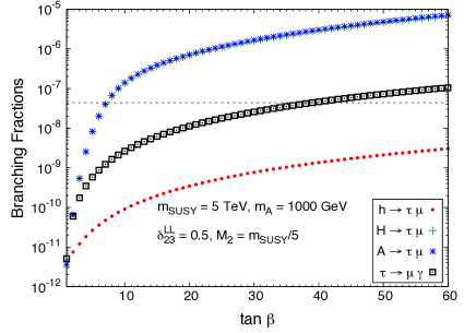
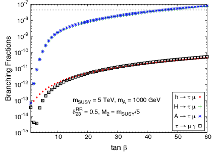
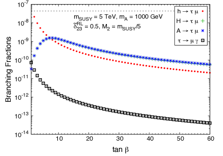
Figure 9.2: BR($h\to\tau\mu$), BR($H\to\tau\mu$), BR($A\to\tau\mu$) and BR($\tau\to\mu\gamma$) for the scenarios defined in Section 5.2.2.2 as functions of $\tan\beta$ for $\delta_{23}^{LL}=$ 0.5 (upper left panel), $\delta_{23}^{RR}=$ 0.5 (upper right panel), $\tilde{\delta}_{23}^{LR}=$ 0.5 (lower left panel) and $\tilde{\delta}_{23}^{RL}=$ 0.5 (lower right panel). In each case, the other flavour changing deltas are set to zero. In all panels, $m_{A}=$ 1000 GeV, $m_{\text{SUSY}}=$ 5 TeV and the other MSSM parameters are set to the values reported in the text, with $M_{2}=m_{\text{SUSY}}/5$. The horizontal dashed line denotes the current experimental upper bound for $\tau\to\mu\gamma$ channel, BR($\tau\to\mu\gamma$) $<4.4\times 10^{-8}$ [212]. The green crosses are overimposed with the blue stars.

As we have said above, we show in Figure 9.2 the behaviour of LFV branching ratios as functions of $\tan\beta$ for $\delta_{23}^{LL}=$ 0.5 (upper left panel), $\delta_{23}^{RR}=$ 0.5 (upper right panel), $\tilde{\delta}_{23}^{LR}=$ 0.5 (lower left panel) and $\tilde{\delta}_{23}^{RL}=$ 0.5 (lower right panel) with $m_{A}=$ 1000 GeV, $m_{\text{SUSY}}=$ 5 TeV and $M_{2}=m_{\text{SUSY}}/5$. All the LFV rates have a very similar behaviour with $\tan\beta$ for both $LL$ and $RR$ mixing cases and grow as $\sim(\tan\beta)^{2}$ for large values of $\tan\beta\gtrsim$ 10, as indicated in the previous paragraphs. In contrast, the LFV rates present a decreasing behaviour with $\tan\beta$ in the $LR$ and $RL$ cases, which are identical. BR$(\tau\to\mu\gamma)$ and BR$(h\to\tau\mu)$ go for all studied $\tan\beta$ values approximately as $\sim(\tan\beta)^{-2}$ while BR$(H\to\tau\mu)$ BR$(A\to\tau\mu)$ grow at low $\tan\beta$ around two orders of magnitude from $\tan\beta=$ 1 to $\tan\beta=$ 5, and from this value decrease in the same way as $\tau\to\mu\gamma$ and $h\to\tau\mu$. Therefore, within the large $\tan\beta$ regime ($\tan\beta\gtrsim$ 10), in the $LL$ and $RR$ mixing cases the LFV rates grow as $\sim(\tan\beta)^{2}$ whilst in the $LR$ and $LR$ ones these rates present the opposite behaviour and decrease as $\sim(\tan\beta)^{-2}$.

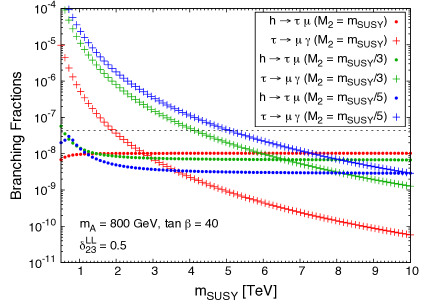
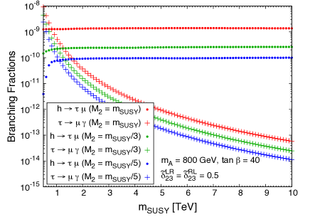
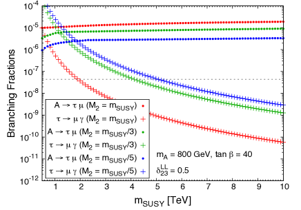
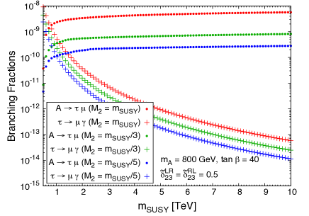
Figure 9.3: Sensitivity to $M_{2}$ for the scenarios defined in Section 5.2.2.2: LFV Higgs decay rates (dots) and BR($\tau\to\mu\gamma$) (crosses) as functions of $m_{\text{SUSY}}$ with $\delta_{23}^{LL}=0.5$ (left panels) and $\tilde{\delta}_{23}^{LR}=\tilde{\delta}_{23}^{RL}=0.5$ (right panels) for different choices of $M_{2}$: $M_{2}=m_{\text{SUSY}}$ (in red), $M_{2}=\frac{1}{3}m_{\text{SUSY}}$ (in green) and $M_{2}=\frac{1}{5}m_{\text{SUSY}}$ (in blue). The results for $H$ (not shown) are nearly identical to those of $A$. In each case, the other flavour changing deltas are set to zero. In all panels, $m_{A}=$ 800 GeV, $\tan\beta=$ 40 and the other MSSM parameters are set to the values reported in the text. The horizontal dashed line denotes the current experimental upper bound for $\tau\to\mu\gamma$ channel, BR($\tau\to\mu\gamma$) $<4.4\times 10^{-8}$ [212].

Now, we are interested in investigating if other choices of $M_{2}$ alter these previous results. For this purpose, we have plotted in Figure 9.3 the predictions of BR($h\to\tau\mu$) (dots in upper panels), BR($A\to\tau\mu$) (dots in lower panels) and BR($\tau\to\mu\gamma$) (crosses in all panels) as functions of $m_{\text{SUSY}}$ for different values of $a$ (see Eq. (5.38)), $a=1$ (in red), $a=\frac{1}{3}$ (in green) and $a=\frac{1}{5}$ (in blue), with $\delta_{23}^{LL}=0.5$ (left panels) and $\tilde{\delta}_{23}^{LR}=\tilde{\delta}_{23}^{RL}=0.5$ (right panels). The results for the $H\to\tau\mu$ channel are nearly identical to those of $A\to\tau\mu$ and not shown here for shortness. In the case of $LL$ mixing, all the LFV Higgs rates, which present the same behaviour with $a$, increase around a factor of 7 from $a=\frac{1}{5}$ to $a=1$, while the $\tau\to\mu\gamma$ rates present the opposite behaviour with $a$, decreasing in a factor about 40 for the same values of $a$. Therefore, if $\delta_{23}^{LL}$ is the responsible for the slepton mixing, and for the explored interval $1/5\leq a\leq 1$, the larger $M_{2}$ is (and consequently $M_{1}$ and $\mu$), the larger the LFV Higgs branching ratios are and the lower BR($\tau\to\mu\gamma$) is. In the $LR$-mixing case we see that again BR($h,H,A\to\tau\mu$) rise as $a$ grows and the enhancement is by a large factor of about 15 by changing $a=\frac{1}{5}$ to $a=1$. In contrast to the $LL$ case, BR($\tau\to\mu\gamma$) also increases with $a$ for $LR$ mixing, although softer than the LFV Higgs rates. In summary, we learn from Figure 9.3 that the best choice, for a fixed delta parameter, in order to obtain the largest LFV Higgs rates is $M_{2}=m_{\text{SUSY}}$. However, we must be very careful, because it is possible that these large rates are excluded by the $\tau\to\mu\gamma$ upper bound, depending basically on the specific values of $\delta_{23}^{LL}$, $\tilde{\delta}_{23}^{LR}$ and $\tan\beta$.

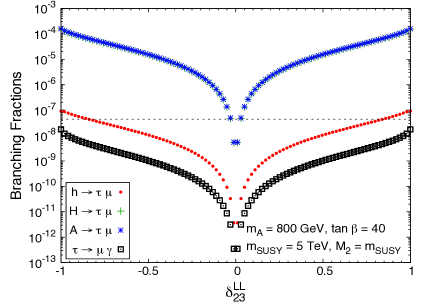
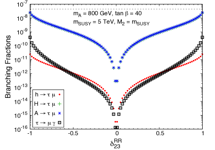
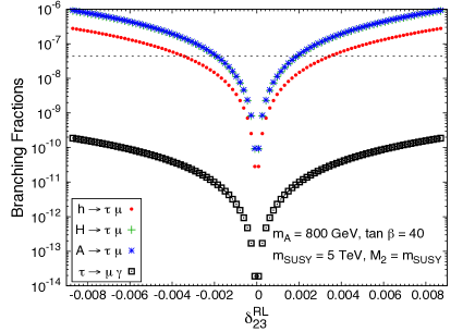
Figure 9.4: BR($h\to\tau\mu$), BR($H\to\tau\mu$), BR($A\to\tau\mu$) and BR($\tau\to\mu\gamma$) for the scenarios defined in Section 5.2.2.2 as functions of $\delta_{23}^{LL}$ (upper left panel), $\delta_{23}^{RR}$ (upper right panel), $\delta_{23}^{LR}$ (lower left panel) and $\delta_{23}^{RL}$ (lower right panel). In each case, the other flavour changing deltas are set to zero. In all panels, $m_{A}=$ 800 GeV, $\tan\beta=40$, $m_{\text{SUSY}}=$ 5 TeV and the other MSSM parameters are set to the values reported in the text, with $M_{2}=m_{\text{SUSY}}$. The horizontal dashed line denotes the current experimental upper bound for $\tau\to\mu\gamma$ channel, BR($\tau\to\mu\gamma$) $<4.4\times 10^{-8}$ [212]. The green crosses are overimposed with the blue stars.

In order to look into the largest values of $\delta_{23}^{AB}$ allowed by data for the choice $M_{2}=m_{\text{SUSY}}$, we show in Figure 9.4 the results of the branching fractions for the LFV Higgs decays into $\tau\mu$ and the related LFV radiative decay $\tau\to\mu\gamma$ as functions of the four deltas considered along this chapter. We have fixed in these plots $\tan\beta=40$. For completeness, we have also presented here the results for $\delta_{23}^{RR}$, which are irrelevant for the present work since all the branching ratios obtained are extremely small to be detectable at the LHC, and the $\delta_{23}^{RL}$ results, which are identical to the $\delta_{23}^{LR}$ ones. The plots in Figure 9.4 show the expected growing of the LFV rates with the $|\delta_{23}^{AB}|$’s, and all of them are clearly symmetric $\delta_{23}^{AB}\to-\delta_{23}^{AB}$. On the upper left panel we have the results for the $LL$ case and it is clear that all the values of $\delta_{23}^{LL}$, from $-1$ to 1, are allowed by data, due to the large suppression that $\tau\to\mu\gamma$ suffers for $m_{\text{SUSY}}=$ 5 TeV. The predictions for $H\to\tau\mu$ (green crosses) are indistinguishable from $A\to\tau\mu$ ones (blue asterisks), which are superimposed in these plots. One can reach values of BR($h\to\tau\mu$) $\simeq 10^{-7}$ and BR($H,A\to\tau\mu$) $\simeq 2\times 10^{-4}$ at the most for $\delta_{23}^{LL}=\pm 1$. The predictions for the LFV rates as functions of $\delta_{23}^{LR}$ are presented on the lower left panel of Figure 9.4. In this case, all the values of $\left|\delta_{23}^{LR}\right|$ are allowed by the $\tau\to\mu\gamma$ upper bound and the largest value of $\left|\delta_{23}^{LR}\right|\simeq$ 0.009 (which corresponds to $\tilde{\delta}_{23}^{LR}\simeq$ 10) gives rise to a branching fraction of $3\times 10^{-7}$ for the $h\to\tau\mu$ channel, while BR($H,A\to\tau\mu$) reach values of $1\times 10^{-6}$. The low rates in the $h\to\tau\mu$ channel for this $LR$-mixing case can be notably increased, as we have said previously, by assuming a lower $\tan\beta$ value closer to the low $\tan\beta$ region with $\tan\beta\lesssim$ 5.

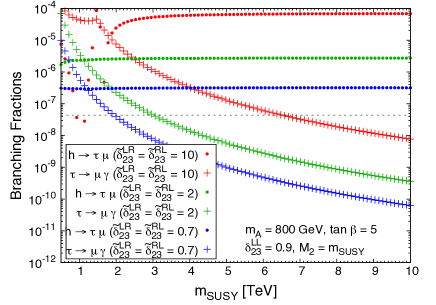
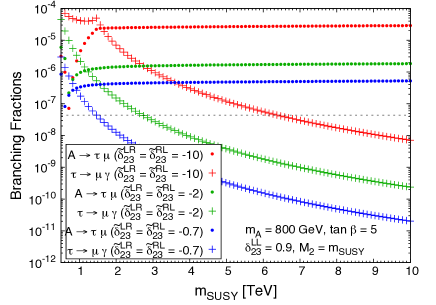
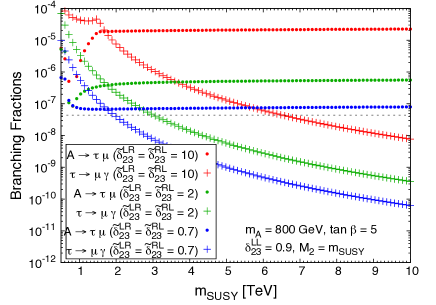
Figure 9.5: Sensitivity to double $LL$ and $LR$ mixing deltas for the scenarios defined in Section 5.2.2.2: LFV Higgs decay rates (dots) and BR($\tau\to\mu\gamma$) (crosses) as functions of $m_{\text{SUSY}}$ with $\delta_{23}^{LL}=0.9$ for different choices of negative $LR$ mixings (left panels), $\tilde{\delta}_{23}^{LR}=\tilde{\delta}_{23}^{RL}$: $-0.7$ (in blue), $-2$ (in green) and $-10$ (in red), and of positive $LR$ mixings (right panels), $\tilde{\delta}_{23}^{LR}=\tilde{\delta}_{23}^{RL}$: $+0.7$ (in blue), $+2$ (in green) and $+10$ (in red). The results for $H$ (not shown) are nearly identical to those of $A$. In each case, the other flavour changing deltas are set to zero. In all panels, $m_{A}=$ 800 GeV, $\tan\beta=$ 5, $M_{2}=m_{\text{SUSY}}$ and the other MSSM parameters are set to the values reported in the text. The horizontal dashed line denotes the current experimental upper bound for $\tau\to\mu\gamma$ channel, BR($\tau\to\mu\gamma$) $<4.4\times 10^{-8}$ [212].

Finally, we have studied the possibility of switching on several deltas simultaneously. Specifically, we have fixed $\delta_{23}^{LL}=0.9$ and considered different choices of $\tilde{\delta}_{23}^{LR}=\tilde{\delta}_{23}^{RL}$ with either negative values: ($-0.7$, $-2$ and $-10$), or positive values ($+0.7$, $+2$ and $+10$). The results are depicted in Figure 9.5 for the case of low $\tan\beta=$ 5 that is the most interesting one since the $LL$ and $LR$ (and $RL$) contributions are of similar size and their interferences can be relevant for some regions of the parameter space. As expected, the four LFV decay rates increase as $|\tilde{\delta}_{23}^{LR}|=|\tilde{\delta}_{23}^{RL}|$ grows, and they are slightly higher than for single $LL$ or $LR$ mixings. The most important conclusion in this case is that we are able to obtain large branching ratios for all the three LFV Higgs decays, reaching values close to $10^{-4}$ for $h$ and about $3\times 10^{-5}$ for $A$ and $H$, if $\tilde{\delta}_{23}^{LR}=\tilde{\delta}_{23}^{RL}=\pm 10$. By comparing the results for negative versus positive $LR$ mixings, we also learn from this figure that there are not relevant differences. The LFV Higgs decay rates for negative mixings are slightly higher than the corresponding rates for positive mixings, and this difference is more visible in the $A$ and $H$ LFV decays than in the $h$ LFV decay. It should also be noted that the rates for $\tau\to\mu\gamma$ decays go the other way around, namely, they are slightly larger for positive $LR$ mixings than for negative $LR$ mixings, indicating that the interference between the $LL$ and $LR$ contributions must be of opposite sign in the LFV Higgs decays versus the $\tau\to\mu\gamma$ decays.

To close this subsection, we can conclude from Figures 9.1, 9.2, 9.3, 9.4 and 9.5 that, for the explored intervals of the parameter space, the largest LFV Higgs rates that are allowed by the $\tau\to\mu\gamma$ upper bound are obtained for the following values of the model parameters: large $m_{\text{SUSY}}\gtrsim$ 5 TeV, $M_{2}$ close to $m_{\text{SUSY}}$ and $|\delta_{23}^{LL}|$ and $|\tilde{\delta}_{23}^{LR}|$ (and/or $|\tilde{\delta}_{23}^{RL}|$) close to their maximum explored values of 1 and 10 respectively. According to these previous findings, in the forthcoming computation of cross sections and event rates at the LHC, whenever we have to fix them, we will set the following particular reference model parameters: $m_{\text{SUSY}}=$ 5 TeV, $M_{2}=m_{\text{SUSY}}$, $\delta_{23}^{LL}=0.9$ and $\tilde{\delta}_{23}^{LR}=\tilde{\delta}_{23}^{RL}=\pm 5$ , which are approximately the largest allowed values by the metastability bounds (see Section 5.2.2.2). The corresponding predictions for other choices of $\delta_{23}^{LL}$, $\tilde{\delta}_{23}^{LR}$, $\tilde{\delta}_{23}^{RL}$, $M_{2}$, $m_{\text{SUSY}}$ and $\tan\beta$ can be easily derived from these commented five figures, from 9.1 to 9.5.

9.4 Results for the LFV cross sections and event rates at the LHC

In this section we present the results of the LFV cross sections and event rates at the LHC which are mediated by the production of neutral MSSM Higgs bosons and their subsequent LFV decays into $\tau\mu$. The scenarios evaluated are the same as in the previous section. The production cross sections of the neutral Higgs bosons are calculated here by means of the code FeynHiggs [238]. For low values of $\tan\beta$, the production cross sections of the three neutral MSSM Higgs bosons are dominated by gluon fusion. By contrast, for moderate and large values of $\tan\beta$ ($\gtrsim 10$), the production cross sections of $H$ and $A$ Higgs bosons via bottom-antibottom quark annihilation become the dominant ones, while the $h$ production cross section is still dominated by gluon fusion. In the following, we consider centre-of-mass energies at the LHC of $\sqrt{s}=$ 8 TeV (current phase) and $\sqrt{s}=$ 14 TeV (future phase) and focus in the two cases with the largest LFV Higgs decay rates, with either $LL$ or $LR$ or both slepton $\tau-\mu$ mixings. Although we do not expect any competitive background to these singular LFV signals at the LHC, a more realistic and devoted study of the potential backgrounds should be done, but this is beyond the scope of this work.

9.4.1 Predictions of LFV cross sections for single $LL$ mixing

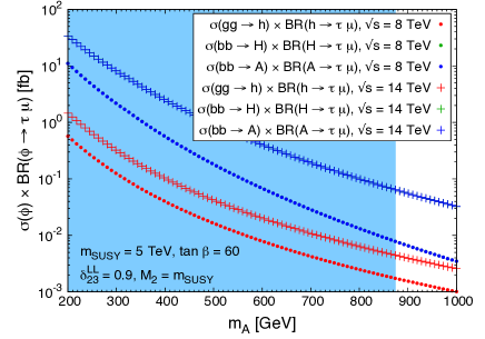
Figure 9.6: LFV cross sections at the LHC for single $LL$ mixing for the scenarios defined in Section 5.2.2.2. Left panel: $\sigma(\phi)$ $\times$ BR($\phi\to\tau\mu$) as a function of $m_{\text{SUSY}}$, where $\phi=h,H,A$, with $m_{A}=$ 1000 GeV and $\tan\beta=$ 60, for $\sqrt{s}=$ 8 TeV (dots) and $\sqrt{s}=$ 14 TeV (crosses). The shaded grey area is excluded by the $\tau\to\mu\gamma$ upper bound. Right panel: $\sigma(\phi)$ $\times$ BR($\phi\to\tau\mu$) as a function of $m_{A}$, where $\phi=h,H,A$, with $\tan\beta=$ 60 and $m_{\text{SUSY}}=$ 5 TeV for $\sqrt{s}=$ 8 TeV (dots) and $\sqrt{s}=$ 14 TeV (crosses). The shaded blue area is excluded by CMS searches for MSSM neutral Higgs bosons decaying to $\tau{\bar{\tau}}$ pairs  [248] in the $m_{A}-\tan\beta$ parameter space for the MSSM $m_{h}^{\text{max}}$ scenario [295][296]. The production cross section of the light Higgs boson $h$ is calculated via gluon fusion and the $H$ and $A$ production cross sections are calculated via bottom-antibottom quark annihilation. In both panels $\delta_{23}^{LL}=$ 0.9 and the other MSSM parameters are set to the values reported in the text, with $M_{2}=m_{\text{SUSY}}$. The green dots and crosses are overimposed with the blue ones.

We first consider the case of single $LL$ mixing which is the delta parameter best motivated from theory. In fact, most of the top-down approaches to LFV physics, where the mixing parameters are generated through RGE running, as for instance in SUSY-seesaw models, predict that the largest mixing comes from $\delta_{23}^{LL}$, with the following hierarchy: $\delta_{23}^{LL}$ $\gg$ $\delta_{23}^{LR}$ $\gg$ $\delta_{23}^{RR}$. This hierarchy can be understood by the solution to the RGE-induced intergenerational mixing, by using the one-loop leading-log approximation where the approximate solution for the off-diagonal terms can be written as [341]:

$$(\Delta m_{\tilde{L}}^{2})_{ij} \,=\,-\frac{1}{8\,\pi^{2}}\,(3\,M_{0}^{2}+A_{0}^{2})\,(Y_{\nu}^{\dagger}\,L\,Y_{\nu})_{ij}\,,$$

$$(\Delta{\cal A}^{l})_{ij} \,=\,-\frac{3}{16\,\pi^{2}}\,A_{0}\,y_{l}\,(Y_{\nu}^{\dagger}\,L\,Y_{\nu})_{ij}\,,$$

$$(\Delta m_{\tilde{E}}^{2})_{ij} \,=\,0\,\,;\,L_{kl}\,\equiv\,\log\left(\frac{M_{X}}{m_{M_{k}}}\right)\,\delta_{kl}.$$ (9.5)

where $i,j,k=1...3$, $m_{M_{k}}$ are the Majorana Masses, $M_{X}$ the GUT scale, $y_{l}$ the Yukawa of the lepton, and $A_{0}$ and $M_{0}$ the universal scalar soft mass and trilinear coupling at the GUT scale. This motivates us to investigate further this case and to look for potential sizeable branching ratios and measurable cross sections at the LHC with just this single $\delta_{23}^{LL}$. In this case, we focus on the large $\tan\beta$ region where, as we have seen previously, the LFV rates are maximized. The most optimistic numbers which we have been able to achieve for $\delta_{23}^{LL}$ are displayed in Figure 9.6, which correspond to the following choice of parameters: $M_{2}=m_{\text{SUSY}}$, $\delta_{23}^{LL}=$ 0.9, $\tan\beta=60$ and $m_{A}=$ 1000 GeV (in order to be in accord with CMS searches [248] for MSSM neutral Higgs bosons decaying to $\tau{\bar{\tau}}$ pairs). On the left panel of Figure 9.6 one can observe the cross sections for all the $h,H,A\to\tau\mu$ channels, for the current LHC phase (dots) and for the future one (crosses), where the shaded grey area is the excluded region by the $\tau\to\mu\gamma$ upper bound. As we can clearly see in this plot, the moderate cross sections predicted in the allowed region of $m_{\text{SUSY}}$ indicate that total integrated luminosities of ${\cal L}\gtrsim 300$ fb^-1 and ${\cal L}\gtrsim 30$ fb^-1 would be required at least for the $H,A\to\tau\mu$ channels, in the current LHC phase and in the future one, respectively, in order to obtain events if the unique source of lepton flavour violation is $\delta_{23}^{LL}$. For the $h\to\tau\mu$ channel it would be needed even larger values of ${\cal L}$, namely, $1\times 10^{3}$ fb^-1 in the present stage of the LHC and 400 fb^-1 in the future one.

The low rates obtained for the $H,A\to\tau\mu$ channels are due to the large value of $m_{A}$ considered up to now, which reduces the production cross sections of these two heavy Higgs bosons. Now we are going to scan over a wider region of $m_{A}$ values, from 200 GeV to 1000 GeV, fixing $m_{\text{SUSY}}$ to our reference value of 5 TeV. The right panel of Figure 9.6 shows the results of $\sigma(\phi)$ $\times$ BR($\phi\to\tau\mu$) as a function of $m_{A}$ with a LHC centre-of-mass energy of $\sqrt{s}=$ 8 TeV (dots) and $\sqrt{s}=$ 14 TeV (crosses). The cross sections of LFV Higgs decays are strongly dependent on $m_{A}$ and fall down more than three orders of magnitude from $m_{A}=$ 200 GeV to $m_{A}=$ 1000 GeV. On one hand, the LFV $H$ and $A$ channels decrease with $m_{A}$, as expected, because this parameter gives precisely the mass of the Higgs particles being produced. On the other hand, the cross section for the $h\to\tau\mu$ process diminishes with this parameter since our settings here lay in the so-called decoupling limit, meaning that for large $m_{A}$ values the lightest Higgs boson $h$ behaves as a SM-like Higgs boson, and in the SM the coupling between the Higgs boson and a $\tau$ and a $\mu$ is zero, therefore leading to extremely suppressed LFV couplings. For low values of $m_{A}\sim$ 200 GeV, we obtain large cross sections, $\sigma(gg\to h)\times$ BR$(h\to\tau\mu)\simeq 0.6\textrm{fb}$ and $\sigma(b\bar{b}\to H,A)\times$ BR$(H,A\to\tau\mu)\simeq 10\textrm{fb}$ in the present LHC phase, and $\sigma(gg\to h)\times$ BR$(h\to\tau\mu)\simeq 2\textrm{fb}$ and $\sigma(b\bar{b}\to H,A)\times$ BR$(H,A\to\tau\mu)\simeq 30\textrm{fb}$ in the future one. However, these low values of $m_{A}$ are not allowed by present LHC data. Indeed, we can see in the shaded area (in blue) of this figure that values of $m_{A}\lesssim$ 875 GeV for $\tan\beta=$ 60 are already excluded by CMS searches for MSSM neutral Higgs bosons decaying to $\tau{\bar{\tau}}$ pairs  [248] in the $m_{A}-\tan\beta$ parameter space for the MSSM $m_{h}^{\text{max}}$ scenario [295][296].

The overall conclusion for the $LL$ case is that, in order to get some Higgs-mediated LFV event at the LHC for $m_{A}$ and $\tan\beta$ input values within the CMS allowed region, total integrated luminosities of ${\cal L}\gtrsim 100$ fb^-1 and ${\cal L}\gtrsim 20$ fb^-1 would be required for the $H,A\to\tau\mu$ channels, in the current LHC phase and in the future one, respectively. For the $h\to\tau\mu$ channel it would be needed larger values of ${\cal L}$: 500 fb^-1 in the present LHC phase and 200 fb^-1 in the future one.

9.4.2 Predictions of LFV cross sections for single $LR$ mixing

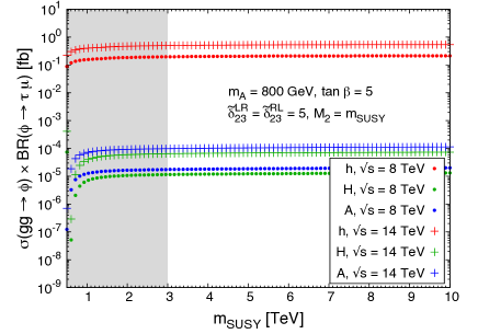
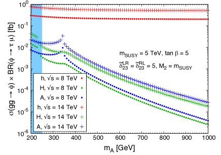
Figure 9.7: LFV cross sections at the LHC for single $LR$ mixing for the scenarios defined in Section 5.2.2.2. Left panel: $\sigma(\phi)$ $\times$ BR($\phi\to\tau\mu$) as a function of $m_{\text{SUSY}}$, where $\phi=h,H,A$, with $m_{A}=$ 800 GeV and $\tan\beta=$ 5, for $\sqrt{s}=$ 8 TeV (dots) and $\sqrt{s}=$ 14 TeV (crosses). The shaded grey area is excluded by the $\tau\to\mu\gamma$ upper bound. Right panel: $\sigma(\phi)$ $\times$ BR($\phi\to\tau\mu$) as a function of $m_{A}$, where $\phi=h,H,A$, with $\tan\beta=$ 5 and $m_{\text{SUSY}}=$ 5 TeV for $\sqrt{s}=$ 8 TeV (dots) and $\sqrt{s}=$ 14 TeV (crosses). The shaded blue area is excluded by CMS searches for MSSM neutral Higgs bosons. The Higgs production cross sections are calculated via gluon fusion. In both panels $\tilde{\delta}_{23}^{LR}=\tilde{\delta}_{23}^{RL}=$ 5 and the other MSSM parameters are set to the values reported in the text, with $M_{2}=m_{\text{SUSY}}$.

Next we consider the case of single $LR$ mixing. For the numerical estimates here we fix $\tilde{\delta}_{23}^{LR}=\tilde{\delta}_{23}^{RL}=$ 5 and focus in the low $\tan\beta$ region where, as we have seen previously, the LFV rates are maximized. The predictions of the cross sections of LFV Higgs processes at the LHC are exhibited in Figure 9.7 for $\sqrt{s}=$ 8 TeV (dots) and $\sqrt{s}=$ 14 TeV (crosses), with $\tan\beta=$ 5 and $M_{2}=m_{\text{SUSY}}$. On the left panel we show the predicted LFV cross sections as functions of $m_{\text{SUSY}}$, with $m_{A}=$ 800 GeV. For the $m_{\text{SUSY}}$ region allowed by the $\tau\to\mu\gamma$ upper bound ($m_{\text{SUSY}}\gtrsim$ 3 TeV), $\sigma(gg\to h)$ $\times$ BR($h\to\tau\mu$) can reach values around 0.2 fb in the present LHC phase and up to 0.5 fb in the future one. The predictions for $\sigma(gg\to H,A)$ $\times$ BR($H,A\to\tau\mu$) are much smaller than the LFV $h$ channel, since the value of $m_{A}$ considered here is rather heavy (800 GeV) and consequently leads to small production cross sections for both $H$ and $A$ Higgs bosons, and reach maximum values of about $10^{-4}$ fb for the future LHC phase, meaning that a total integrated luminosity of at least $10^{4}$ fb^-1 would be required in order to get at least one event.

The results for $\sigma(\phi)$ $\times$ BR($\phi\to\tau\mu$) (with $\phi=h,H,A$) as a function of $m_{A}$ are displayed on the right panel of Figure 9.7 for $m_{\text{SUSY}}=$ 5 TeV. The largest cross section is, by far, for the $h\to\tau\mu$ channel again, even for low values of $m_{A}$. The cusp appearing around $m_{A}\simeq$ 350 GeV for the $A\to\tau\mu$ channel is due to the well known threshold effect when crossing by two on-shell top quarks. This effect also occurs for $H$ production via gluon fusion, but it is softer, resulting in a plateau instead of a cusp. For the LFV $A$ channel, we reach cross sections of 0.01 fb and 0.04 fb at the most in the present and the future LHC phases, respectively, around the top-quark threshold effect, while the largest LFV $H$ cross sections, for values of $m_{A}\lesssim$ 250 GeV, are excluded by CMS searches for MSSM neutral Higgs bosons decaying to $\tau{\bar{\tau}}$ pairs  [248] in the $m_{A}-\tan\beta$ parameter space for the MSSM $m_{h}^{\text{max}}$ scenario [295][296] (shaded blue area). The largest LFV $H$ cross section allowed by CMS searches is $4\times 10^{-3}$ fb ($1\times 10^{-2}$ fb) in the present (future) phase of the LHC. These results show us that, in the future LHC phase, a total integrated luminosity of ${\cal L}=$ 100 fb^-1 could be enough to produce some LFV event coming from the decays of the heavy neutral Higgs bosons. In the case of $h\to\tau\mu$ channel, this same luminosity could give rise to tens of events.

9.4.3 Predictions of LFV cross sections for double $LL$ and $LR$ mixings

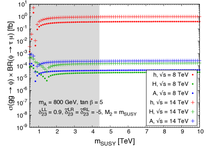
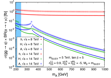
Figure 9.8: LFV cross sections at the LHC for double $LL$ and $LR$ mixings and low $\tan\beta$ for the scenarios defined in Section 5.2.2.2. Left panel: $\sigma(\phi)$ $\times$ BR($\phi\to\tau\mu$) as a function of $m_{\text{SUSY}}$, where $\phi=h,H,A$, with $m_{A}=$ 800 GeV and $\tan\beta=$ 5 for $\sqrt{s}=$ 8 TeV (dots) and $\sqrt{s}=$ 14 TeV (crosses). The shaded grey area is excluded by the $\tau\to\mu\gamma$ upper bound. Right panel: $\sigma(\phi)$ $\times$ BR($\phi\to\tau\mu$) as a function of $m_{A}$, where $\phi=h,H,A$, with $\tan\beta=$ 5 and $m_{\text{SUSY}}=$ 7 TeV for $\sqrt{s}=$ 8 TeV (dots) and $\sqrt{s}=$ 14 TeV (crosses). The shaded blue areas are excluded by CMS searches for MSSM neutral Higgs bosons. The Higgs production cross sections are calculated via gluon fusion. In both panels $\delta_{23}^{LL}=$ 0.9, $\tilde{\delta}_{23}^{LR}=\tilde{\delta}_{23}^{RL}=-5$ and the other MSSM parameters are set to the values reported in the text, with $M_{2}=m_{\text{SUSY}}$.

In this section we present the cross sections of LFV Higgs processes at the LHC in the case of switching on several deltas at the same time. Specifically, we fix $\delta_{23}^{LL}=$ 0.9 and $\tilde{\delta}_{23}^{LR}=\tilde{\delta}_{23}^{RL}=-5$ and focus on both cases with either low or large $\tan\beta$ values. We next present the predictions of the LFV cross sections as functions of $m_{\text{SUSY}}$ and $m_{A}$. Figure 9.8 is devoted to the low $\tan\beta$ case with $\tan\beta=$ 5. Both panels show very similar results to those of Figure 9.7, but it is interesting to notice a slight increase in the LFV cross sections when compared to the previous single $LR$ and $LL$ cases that allow us to require smaller total integrated luminosities in order to get events at the LHC. For example, in the future phase of the LHC, around the top-quark pair production threshold, ${\cal L}\lesssim$ 10 fb^-1 would be enough to obtain one event in the LFV pseudoscalar channel. The $h\to\tau\mu$ channel is even more promising and, for the same LHC phase, with a total integrated luminosity of just 1 fb^-1 we would get already more than one LFV event. As stated in the previous sections, all these rates can be further enhanced if larger values of the $LL$ and/or $LR$ mixings above those here assumed were taken.

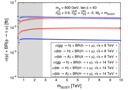
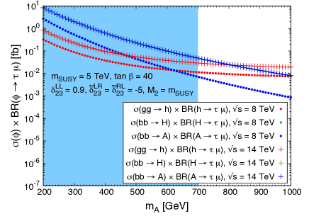
Figure 9.9: LFV cross sections at the LHC for double $LL$ and $LR$ mixings and large $\tan\beta$ for the scenarios defined in Section 5.2.2.2. Left panel: $\sigma(\phi)$ $\times$ BR($\phi\to\tau\mu$) as a function of $m_{\text{SUSY}}$, where $\phi=h,H,A$, with $m_{A}=$ 800 GeV and $\tan\beta=$ 40 for $\sqrt{s}=$ 8 TeV (dots) and $\sqrt{s}=$ 14 TeV (crosses). The shaded grey area is excluded by the $\tau\to\mu\gamma$ upper bound. Right panel: $\sigma(\phi)$ $\times$ BR($\phi\to\tau\mu$) as a function of $m_{A}$, where $\phi=h,H,A$, with $\tan\beta=$ 40 and $m_{\text{SUSY}}=$ 5 TeV for $\sqrt{s}=$ 8 TeV (dots) and $\sqrt{s}=$ 14 TeV (crosses). The shaded blue area is excluded by CMS searches for MSSM neutral Higgs bosons. The production cross section of the light Higgs boson $h$ is calculated via gluon fusion and the $H$ and $A$ production cross sections are calculated via bottom-antibottom quark annihilation. In both panels, $\delta_{23}^{LL}=$ 0.9, $\tilde{\delta}_{23}^{LR}=\tilde{\delta}_{23}^{RL}=-5$ and the other MSSM parameters are set to the values reported in the text, with $M_{2}=m_{\text{SUSY}}$.

The results for the LFV cross sections in the large $\tan\beta$ region are shown in Figure 9.9, for $\tan\beta=$ 40, as functions of $m_{\text{SUSY}}$ (left panel) and as functions of $m_{A}$ (right panel). These results are qualitatively similar to those of Figure 9.6, but the main difference in this case is that all the three LFV cross sections, for $h$, $H$ and $A$, are numerically of the same order of magnitude, due to the enhancement from both $LR/RL$ and $LL$ mixing acting simultaneously and compensating each other in the two studied regions of low and large $\tan\beta$ values. This is particularly interesting for the future LHC phase where we find that a total integrated luminosity of just 50 fb^-1 would be needed to get a few LFV events in either of the three LFV Higgs channels.

9.4.4 Predictions of LFV event rates at the LHC in the $(m_{A},\tan\beta)$ plane

Once we have set up the most relevant parameters for the present study of LFV at the LHC, which are the two flavour mixing deltas $\delta_{23}^{LL}$ and $\delta_{23}^{LR}$ (and correspondingly $\delta_{23}^{RL}$), $m_{\text{SUSY}}$ and $m_{A}$ masses and $\tan\beta$, we will present next the results for the final rates at the LHC, both in the present and future phases, in the most convenient way for comparison with future experimental analysis, namely, in the ($m_{A},\tan\beta$) plane. Since the results for the $H\to\tau\mu$ event rates turn out to be nearly equal to those of the $A\to\tau\mu$ ones will not exhibited them here for shortness. Thus we will focus in the LFV rates of $h$ and $A$ decays. In the following plots we have also specified the areas of the $(m_{A},\tan\beta)$ plane (blue areas) that are excluded by the recent CMS searches for MSSM neutral Higgs bosons decaying to $\tau{\bar{\tau}}$ pairs  [248] in the so-called $m_{h}^{\text{max}}$ scenario [295][296] (variations are possible due to deviations from that scenario, see [296]). All the predictions shown next are allowed by the present upper $\tau\to\mu\gamma$ bound.

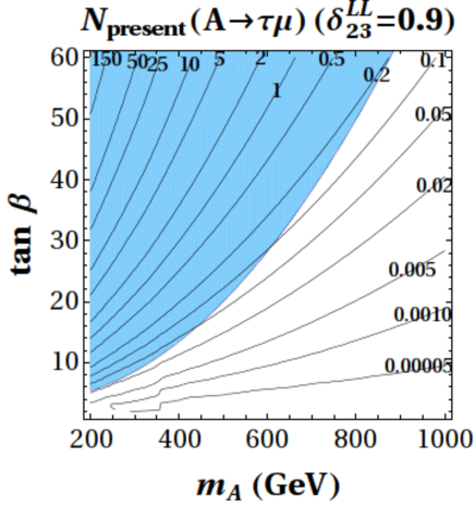
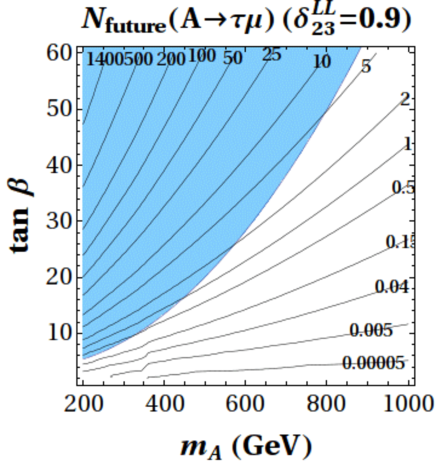
Figure 9.10: Number of expected LFV events in the ($m_{A},\tan\beta$) plane from $A\to\tau\mu$ for $\delta_{23}^{LL}=$ 0.9 and $m_{\text{SUSY}}=$ 5 TeV for the scenarios defined in Section 5.2.2.2. Left panel: present phase of the LHC with $\sqrt{s}=$ 8 TeV and ${\cal L}=$ 25 fb^-1. Right panel: future phase of the LHC with $\sqrt{s}=$ 14 TeV and ${\cal L}=$ 100 fb^-1. In both panels the other MSSM parameters are set to the values reported in the text, with $M_{2}=m_{\text{SUSY}}$. The shaded blue areas are excluded by CMS searches [248] (see variations from these limits for different scenarios in [296]). The results for $H$ (not shown) are nearly equal to these ones for $A$.

We start this analysis with the $LL$ case and plot in Figure 9.10 the number of events expected in the ($m_{A},\tan\beta$) plane for the $A\to\tau\mu$ channel with $\delta_{23}^{LL}=$ 0.9 and $m_{\text{SUSY}}=$ 5 TeV, considering both the present and future LHC phases (left and right panels, respectively). On the other hand, the $h\to\tau\mu$ channel (not shown) cannot supply any significant signal at the LHC in this $LL$ case, as one can infer from Figure 9.6, unless extremely large total integrated luminosities were considered (larger than 500 fb^-1). Due to the CMS exclusion region in the ($m_{A},\tan\beta$) plane [248] for searches of MSSM neutral Higgs bosons decaying to $\tau{\bar{\tau}}$ pairs, it is evident that we cannot expect any LFV event from neither the $h\to\tau\mu$ channel nor the $A,H\to\tau\mu$ channels in the present phase of the LHC if the unique responsible for $\tau-\mu$ mixing is the $\delta_{23}^{LL}$ parameter and $|\delta_{23}^{LL}|<$ 1. The event rates from $A,H\to\tau\mu$ for the future phase of the LHC are more promising, as shown on the right panel of Figure 9.10. For instance, for $m_{A}\simeq$ 450 GeV and $\tan\beta\simeq$ 15, we could expect at least 1 event, and up to 5 for larger values of $m_{A}$ and values of $\tan\beta\gtrsim$ 50.

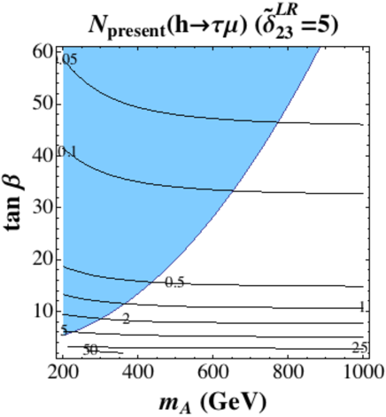
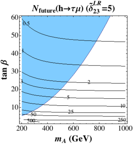
Figure 9.11: Number of expected LFV events in the ($m_{A},\tan\beta$) plane from $h\to\tau\mu$ for $\tilde{\delta}_{23}^{LR}=\tilde{\delta}_{23}^{RL}=$ 5 and $m_{\text{SUSY}}=$ 5 TeV for the scenarios defined in Section 5.2.2.2. Left panel: present phase of the LHC with $\sqrt{s}=$ 8 TeV and ${\cal L}=$ 25 fb^-1. Right panel: future phase of the LHC with $\sqrt{s}=$ 14 TeV and ${\cal L}=$ 100 fb^-1. In both panels the other MSSM parameters are set to the values reported in the text, with $M_{2}=m_{\text{SUSY}}$. The shaded blue areas are excluded by CMS searches [248] (see variations from these limits for different scenarios in [296]).

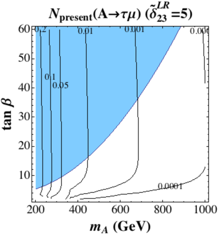
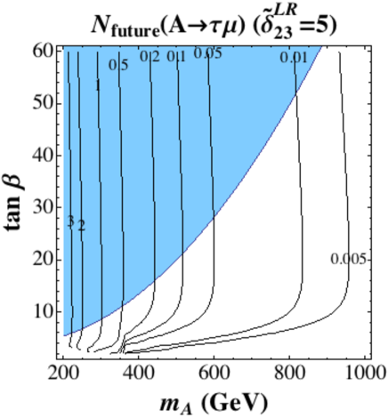
Figure 9.12: Number of expected LFV events in the ($m_{A},\tan\beta$) plane from $A\to\tau\mu$ for $\tilde{\delta}_{23}^{LR}=\tilde{\delta}_{23}^{RL}=$ 5 and $m_{\text{SUSY}}=$ 5 TeV for the scenarios defined in Section 5.2.2.2. Left panel: present phase of the LHC with $\sqrt{s}=$ 8 TeV and ${\cal L}=$ 25 fb^-1. Right panel: future phase of the LHC with $\sqrt{s}=$ 14 TeV and ${\cal L}=$ 100 fb^-1. In both panels the other MSSM parameters are set to the values reported in the text, with $M_{2}=m_{\text{SUSY}}$. The shaded blue areas are excluded by CMS searches [248] (see variations from these limits for different scenarios in [296]). The results for $H$ (not shown) are nearly equal to these ones for $A$.

Next we analyze the results for the case of $LR$ and $RL$ mixings in the ($m_{A},\tan\beta$) plane. Figures 9.11 and 9.12 summarize the results for the $h\to\tau\mu$ and $A\to\tau\mu$ channels, respectively, in the present and future LHC stages.

On the left panel of Figure 9.11, where the number of expected events from the $h\to\tau\mu$ channel in the present phase of the LHC are shown as a function of $m_{A}$ and $\tan\beta$, for $m_{\text{SUSY}}=$ 5 TeV and $\tilde{\delta}_{23}^{LR}=\tilde{\delta}_{23}^{RL}=$ 5, we see again that the maximum allowed number of events are obtained in the low $\tan\beta$ region. Tens of events are expected, up to 50 for $\tan\beta\lesssim$ 3, in all the studied $m_{A}$ interval. In any case, in all the allowed region the number of predicted events are softly dependent on $m_{A}$ and at least one event is obtained, even for large values of $m_{A}$ and $\tan\beta\lesssim$ 10. On the right panel of Figure 9.11, the predictions for the $h\to\tau\mu$ channel, in the future LHC phase with a centre-of-mass energy of $\sqrt{s}=$ 14 TeV and a total integrated luminosity of ${\cal L}=$ 100 fb^-1, show the same behaviour with respect to the two pair of parameters as on the left panel but with an increase in the number of events of around one order of magnitude. Again the maximum amount of events are for the lowest $\tan\beta$ values, being these nearly independent on $m_{A}$, and the rates decrease as we raise $\tan\beta$, showing a small variation with respect to $m_{A}$ for the allowed region by data (in white), as in the previous mentioned plot. Specifically, we obtain up to 500 events for $\tan\beta\simeq$ 2, and between 250 and 1 events for the region between $\tan\beta=$ 2 and $\tan\beta=$ 35.

The corresponding results for the $A\to\tau\mu$ channel, displayed in Figure 9.12, show a very different behaviour with $m_{A}$ and $\tan\beta$ than the previous $h$ case. The number of expected LFV events at the LHC via $A\to\tau\mu$ decays diminish as $m_{A}$ increases, due to the suppression in the production cross section of a heavy pseudoscalar Higgs boson, and stay constant with $\tan\beta$, due mainly to the compensation between the growing of the $A$ production cross section via bottom-antibottom quark annihilation and the reduction of BR$(A\to\tau\mu)$ with this parameter, as previously illustrated in Figure 9.2. In the present phase of the LHC we cannot expect any event, as shown on the left panel of Figure 9.12. The right panel of Figure 9.12, containing the predictions for the $A\to\tau\mu$ channel in the future LHC phase, shows an analogous behaviour to that of the left panel. The number of expected events increase around one order of magnitude respect the present LHC phase, and for values of $m_{A}$ below 300 GeV, one could expect between 1 and 3 events independently on the value of $\tan\beta$.

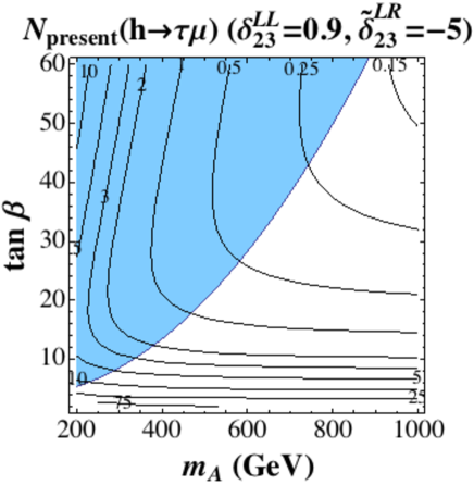
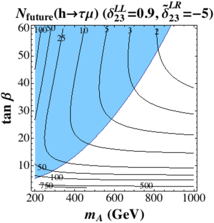
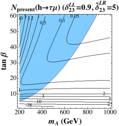
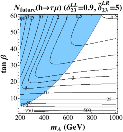
Figure 9.13: Number of expected LFV events in the ($m_{A},\tan\beta$) plane from $h\to\tau\mu$ for $m_{\text{SUSY}}=$ 5 TeV, $\delta_{23}^{LL}=$ 0.9 and $\tilde{\delta}_{23}^{LR}=\tilde{\delta}_{23}^{RL}=$ -5 (upper panels) or $\tilde{\delta}_{23}^{LR}=\tilde{\delta}_{23}^{RL}=$ +5 (lower panels) for the scenarios defined in Section 5.2.2.2. Left panels: present phase of the LHC with $\sqrt{s}=$ 8 TeV and ${\cal L}=$ 25 fb^-1. Right panels: future phase of the LHC with $\sqrt{s}=$ 14 TeV and ${\cal L}=$ 100 fb^-1. In all panels the other MSSM parameters are set to the values reported in the text, with $M_{2}=m_{\text{SUSY}}$. The shaded blue areas are excluded by CMS searches [248] (see variations from these limits for different scenarios in [296]).

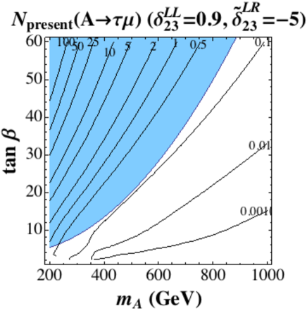
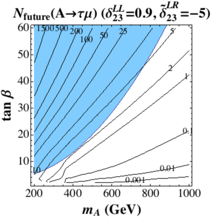
Figure 9.14: Number of expected LFV events in the ($m_{A},\tan\beta$) plane from $A\to\tau\mu$ for $\delta_{23}^{LL}=$ 0.9, $\tilde{\delta}_{23}^{LR}=\tilde{\delta}_{23}^{RL}=$ -5 and $m_{\text{SUSY}}=$ 5 TeV for the scenarios defined in Section 5.2.2.2. Left panel: present phase of the LHC with $\sqrt{s}=$ 8 TeV and ${\cal L}=$ 25 fb^-1. Right panel: future phase of the LHC with $\sqrt{s}=$ 14 TeV and ${\cal L}=$ 100 fb^-1. In both panels the other MSSM parameters are set to the values reported in the text, with $M_{2}=m_{\text{SUSY}}$. The shaded blue areas are excluded by CMS searches [248] (see variations from these limits for different scenarios in [296]). The results for $H$ (not shown) are nearly equal to these ones for $A$.

Finally, the results for the $h\to\tau\mu$ and $A\to\tau\mu$ channels in the double $LL$ and $LR$ mixings case are summarized in Figures 9.13 and 9.14, respectively.

The predictions for the contour lines of $h\to\tau\mu$ event rates (Figure 9.13) show a clear different pattern than in the previous cases of single deltas. In both LHC phases, we achieve an increase in the number of events respect to the single $LL$ and $LR$ (and/or $RL$) mixing cases. The most interesting numbers are at the lower part of these plots with $\tan\beta<10$. We find as large as 75 LFV events in the present phase of the LHC for very low values of $\tan\beta\simeq$ 2 and $m_{A}\lesssim$ 600 GeV. In the future LHC phase we predict up to 750 events, for $\tan\beta\simeq$ 2 and $m_{A}\lesssim$ 450 GeV. It should be also noted that these conclusions apply to both choices for the $LR/RL$ mixings of -5 and +5, as can be seen in Figure 9.13. The only notable differences that we find between the results of these two cases are in the slight different patterns of the contour lines, signalling a small different sensitivity to $m_{A}$ and/or $\tan\beta$. Also one can appreciate in these plots that one gets a bit lower rates for +5 than for -5, in agreement with our previous findings reported in Figure 9.5

The number of events for the $A\to\tau\mu$ channel in the double $LL$ and $LR$ mixings case are displayed in Figure 9.14. The $LL$ mixing is set here to 0.9 and the $LR=RL$ mixings are fixed to -5. As expected, the predicted event rates increase as $\tan\beta$ grows and are reduced as $m_{A}$ gets bigger, due to the suppression in the production cross section of a heavy pseudoscalar Higgs boson. However, for the present LHC phase one cannot say much about this channel, since all the $m_{A}-\tan\beta$ regions which could produce a relevant number of LFV events are excluded at present by CMS searches. We find at the most one event in the tiny low left corner of the allowed region in this $(m_{A},\tan\beta)$ plot. In contrast, the predictions in the future phase of the LHC are more promising. We predict up to about 5 LFV events for large values of $m_{A}$ and $\tan\beta$ and up to 10 in the low $\tan\beta$ region with $m_{A}\simeq$ 200 GeV. Similar conclusions are found for the case of positive $LR$=+5 mixing (not shown). The shape of the contour lines in this case are slightly modified at low $\tan\beta$ but with no relevant implications in terms of event rates.

Chapter 10 Conclusions

The recent discovery of the Higgs boson, if it is confirmed that is indeed the SM Higgs boson, would close the particle content of the SM, and would establish the Brout-Englert-Higgs mechanism as the correct way of breaking the $SU(2)_{L}\times U(1)_{Y}$ electroweak symmetry and giving mass to the elementary particles. However the SM is not the final model of particle physics since it is believed to be an effective theory of a wider and more complete theory, with new features as for example: including gravity in its framework, explaining the more fundamental dynamical origin for the value of the masses and couplings of the particles and the cause of dark matter, probably unifying the forces, and giving an answer to other unknown phenomena. The absence of any direct signal of such a wider theory in the experiments so far, has lead us in the present work to study observables where it could be possible to observe indirect effects of this new physics before it is directly discovered.

Flavour physics has been during the history of Particle Physics a unique place from where to extract clues and information about non yet discovered particles, as it happened before the discovery of the top quark or the masses of the neutrinos, and thus flavour has been our choice through this work where to look for these new physics effects. This choice has been done in combination with the new observation subject that is the Higgs boson, whose properties as mass, couplings or decay rates, still unknown or measured with low precision could reveal us surprises, departing from the SM-like behaviour that until the moment seems to exhibit the present data.

The model of new physics studied through this work has been the MSSM. Within this model we have carried out a research on the most relevant phenomenology implied by the hypothesis of NMFV from general flavour mixing in the sfermion sector both for squarks and sleptons. In order to do this, in Chapter 5 we have introduced a general parametrization of the flavour mixing elements between different sfermion generations in terms of a series of generic and dimensionless parameters $\delta^{XY}_{ij}$ ($X,Y=L,R$; $i$ and $j$ are the generations involved in the mixing), and then we have explored through this thesis the consequences of these parameters on various observables.

The first part of our research has been focused on the squark sector. Chapter 6 was devoted to the study of the flavour mixing between the second and the third generation squarks, through the following $B$ physics observables: ${\rm BR}(B\to X_{s}\gamma)$, ${\rm BR}(B_{s}\to\mu^{+}\mu^{-})$ and $\Delta M_{B_{s}}$. We have studied the phenomenology of these observables with respect to the MSSM and the $\delta^{XY}_{ij}$ parameters, and constrained these latter with the last experimental observations. It has also been compared the situation before and after the LHC. The numerical evaluation of these observables has been done with the BPHYSICS subroutine of the SuFla code, to which we have added the one-loop gluino boxes contribution in the case of the $\Delta M_{B_{s}}$, that was previously not available and it is known to be relevant in the context of NMFV scenarios. We have estimated the size of these corrections and compared them with the other relevant contributions from chargino boxes and double Higgs penguins for all values of $\tan\beta$ for the first time. We have concluded that gluino boxes dominate for moderate and low $\tan\beta\leq 20$, while at large $\tan\beta$ the double $H$-penguins dominate. For the other observables, the large $\tan\beta$ effects could also very relevant specially because of the effects of the gluino and chargino loops in the case of ${\rm BR}(B\to X_{s}\gamma)$, and of the Higgs penguin diagrams for ${\rm BR}(B_{s}\to\mu^{+}\mu^{-})$. The constraints for the studied scenarios from each of the $B$ physics observables to the $\delta^{XY}_{ij}$ before and after the LHC data can be found in tables 6.1 and 6.3 respectively. In tables 6.2 and 6.4 one can find the combined constraints of the three observables for the pre-LHC and post-LHC situations respectively. From this study, we have also concluded that ${\rm BR}(B\to X_{s}\gamma)$ and $\Delta M_{B_{s}}$ are the most restrictive observables.

The absence of SUSY in the LHC so far has moved the allowed values of the masses of the sparticles to higher energy regions. The scenarios studied for the pre-LHC situation have lighter squarks than are not allowed anymore in the post-LHC situation, and thus the corrections to the $B$ physics observables are smaller for the latter, and consequently the allowed regions for the deltas are at present larger than they were before the LHC started.

For the pre-LHC situation, the NMFV deltas in the top-sector could be sizeable $|\delta_{ct}^{XY}|$ larger than ${\cal O}(0.1)$ and still compatible with $B$ data. In particular, $\delta^{RL}_{ct}$ and $\delta^{RR}_{ct}$ were the less constrained parameters, and to a lesser extent also $\delta^{LR}_{ct}$. The parameters on the bottom-sector were, in contrast, quite constrained. The most tightly constrained were clearly $\delta^{LR}_{sb}$ and $\delta^{RL}_{sb}$, specially the first one with just some singular allowed values: either positive and of the order of $3-5\times 10^{-2}$, or negative and with a small size of the order of $-7\times 10^{-3}$; for the second the limits were around $2\times 10^{-2}$ for both positive and negative values. $\delta^{RR}_{sb}$ was the less constrained parameter in the bottom sector, with larger allowed intervals of $|\delta^{RR}_{sb}|\mathrel{\;{\hbox{\raise 1.50696pt\hbox{$<$}}\kern-3.8889pt\kern-3.8889pt\hbox{\lower 2.79857pt\hbox{$\sim$}}}\;}0.4-0.9$ depending on the scenario. For the current post-LHC situation, the less restricted deltas are $\delta^{RR}_{ct}$ and $\delta^{RR}_{sb}$ than in general could reach a size of ${\cal O}(1)$, then $\delta^{LL}_{23}$, $\delta^{LR}_{ct}$ and $\delta^{RL}_{ct}$ with bounds one order of magnitude smaller, with the first one being more restricted than the last two, and finally the most restricted deltas are $\delta^{LR}_{sb}$ and $\delta^{RL}_{sb}$ that can reach $|\delta^{XY}_{ij}|$ at most of ${\cal O}(0.01)$.

In general terms the sensitivity of ${\rm BR}(B\to X_{s}\gamma)$ follows the behaviour we just described for the different deltas. For $\Delta M_{B_{s}}$ it is possible to find more or less sensitivity to each different delta depending on the point of study in the MSSM parameter space, due mainly to the different contributions as the gluino boxes and the double Higgs penguins, with very different behaviour with $\tan\beta$, as explained before. Although we remark again than in general large sensitivity is found. In the case of ${\rm BR}(B_{s}\to\mu^{+}\mu^{-})$, the main sensitivity is to $\delta^{LL}_{23}$, and then depending on the MSSM point also to the other deltas. This behaviour with $\delta^{LL}_{23}$ depends to a great extent of the enhancement at large $\tan\beta$, but the present experimental constraints force $M_{A}$ to be large in this last case, producing a decrease on the sensitivity to the delta that can counteract the former effect.

From the numerical evaluations it could also be observed than some excluded MSSM points with MFV (i.e. for vanishing deltas) by $B$ physics observables could be recovered as allowed scenarios after setting some of the deltas to non-zero values.

After having a general picture of the restrictions of the different deltas by the $B$ physics observables, and the behaviour of these observables, we have considered in Chapter 7 the corrections to the Higgs boson mass generated from squark flavour mixing from these same deltas. In first place, we performed an analytical study on these corrections, deriving the one-loop formulas for them with FeynArts and FormCalc. The new Feynman rules included in the model file are listed in the Appendix A, and all the results for the unrenormalized self-energies and tadpoles are collected in Appendix B. In the MFV case, up to three loop corrections to the neutral Higgs bosons masses are available, but the study of the NMFV case has been restricted in the past to the study of some particular flavour mixing elements, as the one-loop calculation taking into account the $LL$-mixing between the third and second generation of scalar up-type quarks. Our one-loop study in this thesis has been done in full generality, including all generations and all flavour mixing terms for the up- and down-type of squarks. We have also checked with this generality the finiteness of the analytical results for these renormalized Higgs self-energies. These corrections presented in the Appendix B have been compared with the code included in FeynHiggs, and in the process of checking the finiteness of the formulas we have found discrepancies with the charged Higgs part of FeynHiggs, leading to an updated version of the code.

The next step has been a numerical evaluation of the Higgs bosons mass corrections from squark flavour mixing between the second and the third generation, taking into account the restrictions from the $B$ physics observables of the previous chapter. The numerical evaluation has been performed for the cases of having one or two $\delta^{XY}_{ij}$ with a non-zero value, comparing the situation previous and following to the LHC data. With respect to the one delta studies, it can be seen from our plots (see for instance figs. 7.1, 7.2 and 7.3) how the corrections to all masses are symmetric in the sign of the deltas, as a difference of what happened with the $B$ physics observables, and that can be positive or negative depending on the scenario and the value of the delta. In particular for the light Higgs boson, the corrections tend to have an “M form”, being positive and small for small deltas, and then negative and larger in size as the deltas grow. For the pre-LHC situation, we have found a very strong sensitivity to $\delta^{LR}_{sb}$ and $\delta^{RL}_{sb}$ for all the Higgs bosons, that are also the most constrained deltas from $B$ physics. For the light Higgs boson we found also an important sensitivity to $\delta^{LR}_{ct}$ and $\delta^{RL}_{ct}$, reaching values of up to tens of GeV for the low $\tan\beta$ case where the $B$ physics observables are less restrictive. For the post-LHC situation, the general behaviour of the corrections with the various deltas remains approximately the same. The values of the corrections are very large as compared with the precision of the LHC, and should be taken into account into any Higgs boson analysis in the NMFV framework. In fact, we find that the LHC is able to put constraints on some of these delta parameters like $\delta^{LR}_{ct}$ and $\delta^{RL}_{ct}$ that are allowed by other observables, as it is the case for the $B$ physics observables.

The numerical analysis has been extended for the light Higgs boson corrections to the case of having simultaneously two deltas with non-zero values, in the pre-LHC situation. The largest corrections allowed by $B$ data have been found for the $(\delta^{LL}_{23},\delta^{LR}_{ct})$ and $(\delta^{LL}_{23},\delta^{RL}_{ct})$ cases. These corrections have reached several tens of GeV in the pre-LHC situation. The largest allowed region by $B$ data and largest corrections have corresponded to scenarios with low $\tan\beta$ and heavy SUSY spectra. Also important corrections have been found in the $(\delta^{LL}_{23},\delta^{RR}_{ct})$ plane up to tens of GeV for some specific points. The corrections found to the heavy Higgs bosons in the double delta plane have been much smaller than the previous ones.

The next part of our research, has been the study of the slepton flavour mixing. In Chapter 8 we have developed a study of the phenomenology on different LFV observables and concluded with the constraints that they set on the flavour mixing parameters $\delta^{AB}_{ij}$ of the slepton sector. The LFV processes whose phenomenology have been studied in this chapter have been: radiative decays $\mu\to e\gamma$, $\tau\to e\gamma$ and $\tau\to\mu\gamma$ ($l_{j}\to l_{i}\gamma$), leptonic decays $\mu\to 3e$, $\tau\to 3e$ and $\tau\to 3\mu$ ($l_{j}\to 3l_{i}$), semileptonic tau decays $\tau\to\mu\eta$ and $\tau\to e\eta$ and conversion of $\mu$ into $e$ in heavy nuclei. The radiative decays are usually the most restrictive ones, but the leptonic and semileptonic decays are included because they give access to the Higgs sector parameters, since they can be mediated by Higgs bosons. Our numerical study has been done for scenarios that are allowed by the last data from the LHC, including a mass for the light Higgs boson around 125 - 126 GeV, and also the current value for the muon anomalous magnetic moment, $(g-2)_{\mu}$.

Our study has shown that the radiative decays are still the most restrictive observables to the slepton flavour mixing parameters. Comparing the flavour mixings between different pairs of generations, the experimental bounds for the observables related with the 12-mixings are around four orders of magnitude smaller than the others in all observables, and thus these mixings are much more constrained. The bounds for 23-mixings are similar to the ones for 13-mixings. It was also shown that all the observables behave symmetrically respect to the sign of the deltas. The constraints for the different $\delta^{AB}_{ij}$ for the studied points are collected in Tab. 8.1. The most restrictive constraints to $LL$ and $RR$ mixings have been found to happen for the large $\tan\beta$ case, while the $LR$ mixings are independent of $\tan\beta$ and have stronger constraints for the cases with lightest sleptons.

We also found that the effect of the pseudoscalar Higgs boson mediation in the semileptonic tau decays was not very important since the present exclusion limits for the mass of this Higgs boson lead us to assume a quite heavy $A$ boson, whose effects are then reduced. These observables set no constraints to the 23- and 13-mixings. With respect to the photon mediation in the leptonic decays and in the conversion of $\mu$ into $e$ in heavy nuclei, we confirmed that this photon channel dominates over the other contributions, and thus there was a correlation between the predictions for the leptonic decay rates, the $\mu-e$ conversion rates and the radiative decay rates.

After this, our study was extended to the case of having simultaneously two deltas different from zero. First we studied the case $(\delta^{AB}_{23},\delta^{CD}_{23})$ with $AB\neq CD$ and found constructive or destructive interferences on ${\rm BR}(\tau\to\mu\gamma)$ depending on the signs of the deltas. The most relevant case was $(\delta^{LR}_{23},\delta^{LL}_{23})$ where important destructive interferences were found for the case of opposite signs of the deltas, that made larger the maximum allowed value for each delta as compared with having just that delta. The shape and size of the allowed regions with extreme solutions as $(\pm 0.9,\mp 0.9)$ for the deltas came from our full mass matrix diagonalization computation, and thus they can not be described with the simplest MIA formulas that are usually used in the literature. As a second study on the two-delta plane, we studied the constraints in the (13,23) mixings coming from $\mu\to e\gamma$ and $\mu-e$ conversion as compared with the bounds coming from the observables related to each single delta, and found surprisingly better constraints from this double delta situation.

The study on the bounds on slepton flavour mixings from the radiative decays was completed with a study on the dependence of the bounds on the deltas with respect to the most relevant MSSM parameters in this LFV context: $\tan\beta$ and the mass scale of the sleptons $m_{\rm SUSY}$. The study of the bounds was done comparing it with the allowed regions by the measurements of the Higgs boson mass and the value of $(g-2)_{\mu}$. We observed how the maximal allowed values on the $\delta^{LL}_{ij}$’s and $\delta^{RR}_{ij}$’s scale with $m_{\rm SUSY}$ and $\tan\beta$ approximately growing with increasing $m_{\rm SUSY}$ as $\sim m_{\rm SUSY}^{2}$ and decreasing with increasing (large) $\tan\beta$ as $\sim 1/\tan\beta$. The maximal allowed values of the $\delta^{LR}_{ij}$’s (and similarly $\delta^{RL}_{ij}$’s) are independent on $\tan\beta$ and grow approximately as $\sim m_{\rm SUSY}$ with increasing $m_{\rm SUSY}$. It was also observed how $(g-2)_{\mu}$ requires a rather light SUSY-EW sector, i.e. light charginos, neutralinos and sleptons, and a rather large $\tan\beta$, and $M_{h}$ requires a rather heavy SUSY squark sector, creating some tension between the two observables when the slepton and the squark sector were related, as it happened in our scenarios.

The maximum values for the deltas found for our scenarios in the favoured by LHC and $(g-2)_{\mu}$ data MSSM parameter space region, lay at the following intervals: $|\delta^{LL}_{12}|_{\rm max}\sim{\cal O}(10^{-5},10^{-4})$, $|\delta^{LR}_{12}|_{\rm max}\sim{\cal O}(10^{-6},10^{-5})$, $|\delta^{RR}_{12}|_{\rm max}\sim{\cal O}(10^{-3},10^{-2})$, $|\delta^{LL}_{23}|_{\rm max}\sim{\cal O}(10^{-2},10^{-1})$, $|\delta^{LR}_{23}|_{\rm max}\sim{\cal O}(10^{-2},10^{-1})$, $|\delta^{RR}_{23}|_{\rm max}\sim{\cal O}(10^{-1},10^{0})$. Very similar general bounds as for the 23 mixing are found for the 13 mixing.

Our work was concluded with Chapter 9, where we studied the effects on LFV Higgs decays from slepton flavour mixing. This research was done focusing on the possibility of a very heavy SUSY spectra above the TeV scale and we were mainly motivated in looking for SUSY non-decoupling effects in the LFV Higgs decays being governed by the general slepton flavour mixing.

The observables chosen for this last study in this thesis were the LFV Higgs decays $\phi\to\tau\mu$, with $\phi=h,H,A$, and the LFV radiative decay $\tau\to\mu\gamma$. Similar results and conclusions can be extrapolated for the $\phi\to\tau e$ and $\tau\to e\gamma$ decays. As we saw in the previous chapter, the $\tau\to\mu\gamma$ radiative decay was the most constraining one of our studied observables to the slepton flavour mixing between the second and the third generations. The LFV Higgs couplings to leptons are proportional to the heaviest lepton mass involved, and thus we were more interested on the decays to $\tau$ than to other leptons. Besides we saw in the previous chapter that the constraints from $\mu\to e\gamma$ on the slepton flavour mixings are very tight and therefore do not lead to measurable $\phi\to\mu e$ rates. The predictions for the $\phi\to\tau e$ decay are very similar to the ones for the $\phi\to\tau\mu$ decays, and from the experimental point of view the sensitivity is also very similar, so our results are easily translated into this other channel.

The numerical evaluation of our study has been done with SPHENO and a private FORTRAN code, where we have implemented the full one-loop formulas for the LFV Higgs and radiative decays. The spectrum of the Higgs sector and the total widths of the Higgs bosons have been calculated as before with FeynHiggs at two-loop order.

We have shown that the three LFV Higgs decays $\phi\to\tau\mu$, with $\phi=h,H,A$, present a non-decoupling behaviour with $m_{\text{SUSY}}$, remaining constant at large $m_{\text{SUSY}}>2$ TeV. This is complemented with the radiative decays behaviour showing on the contrary a fast decoupling with $m_{\text{SUSY}}$. Thus we have an optimal situation for detecting indirectly the effects of SUSY even with a very heavy SUSY spectra scale. With respect to other parameters, the branching ratios grow at large $\tan\beta$ as BR($h,H,A\to\tau\mu$) $\sim(\tan\beta)^{2}$ for the $LL$ and $RR$ case, and decrease as $(\tan\beta)^{-2}$ in the $\tilde{\delta}_{23}^{LR}$ case. The most relevant $\delta_{23}^{AB}$ parameter at low $\tan\beta$ values for the lightest Higgs boson $h$ is ${\tilde{\delta}}_{23}^{LR}$, which gives rise to larger LFV Higgs decay rates than $\delta_{23}^{LL}$ and $\delta_{23}^{RR}$, whereas for the $H$ and $A$ Higgs bosons the most relevant parameter is $\delta_{23}^{LL}$. At large $\tan\beta$ values, the most relevant parameter for all the three Higgs bosons is $\delta_{23}^{LL}$. It was also shown that by taking large $M_{2}=\mu$ the branching ratios were also enhanced. With respect to $M_{A}$ it would be desirable to have a low $M_{A}$ in the case of large $\tan\beta$ to enhance the branching ratio of the heavy Higgs bosons, but the exclusion limits in the $M_{A}-\tan\beta$ plane make it impossible.

The results were shown to be symmetric respect to the sign of the $\delta_{23}^{AB}$, and equal for ${\tilde{\delta}}_{23}^{LR}$ and ${\tilde{\delta}}_{23}^{RL}$. And we also saw that considering two $\delta_{23}^{AB}$ different from zero produced interferences that could enhance or reduce branching ratios.

This chapter was concluded with a computation of the LFV event rates that will be produced by these $\phi\to\tau\mu$ decays at the LHC in the $M_{A}-\tan\beta$ plane with large $m_{\text{SUSY}}\geq 5$ TeV, considering the present phase with a centre-of-mass energy of $\sqrt{s}=$ 8 TeV and the future phase with $\sqrt{s}=$ 14 TeV. For the single mixing cases, we concluded that the $RR$ mixing will not be able to be measured at the LHC. The $LL$ case would produce up to 5 events for the heavy Higgs bosons decays in the future phase of the LHC at large $\tan\beta$, and none for the light Higgs boson. And finally $LR$ is found to be the most relevant parameter, producing up to 50 events for $m_{\text{SUSY}}\geq 5$ TeV for low $\tan\beta$ for the light Higgs boson in the present phase, and hundreds of events in the future phase. In the case of the heavy Higgs bosons we obtained a few events only in the future phase. All these results are of course allowed by the relevant radiative decay $\tau\to\mu\gamma$.

In the double-mixing case, the best situation was found for the case of $LL$ and $LR$ mixings. In this case the sensitivity with respect to $\tan\beta$ was improved, and we obtained for instance, a few events for the light Higgs boson at the present stage of the LHC even for moderate $\tan\beta\sim 15$ and large $m_{A}\geq$ 500 GeV. In the future LHC phase the reach to larger $\tan\beta$ values increased and we got some event even at very large $\tan\beta\sim 40$ and $m_{A}\geq$ 800 GeV. The largest rates found in this double-mixing situation were in any case for $h\to\tau\mu$ and were clearly localised at the low $\tan\beta$ region where we predicted for the present LHC phase up to about 75 events, and up to about 750 LFV events for the future LHC phase. In the future LHC phase, we got about 10 events at the most for the $H,A\to\tau\mu$ channels in the low $\tan\beta$ region and 5 events at the most in the high $\tan\beta$ region.

As a summary of our work, we have presented an exhaustive study of the phenomenological implications from general sfermion flavour mixing in a NMFV-MSSM context on $B$ physics observables, Higgs bosons masses corrections, LFV in leptonic observables and LFV Higgs decays. Through our study, we have set constraints on the sfermion flavour mixing parameters from the last experimental measurements. With respect to the Higgs bosons, it has been shown the important effects of the squark flavour mixing in the value of the Higgs bosons masses, and the possibility of using the value of the masses to set constraints on the squark flavour mixing. We have also shown how LFV Higgs decays are unique observables to indirectly test SUSY even in the experimentally discouraging situation of having a very heavy supersymmetry not directly reachable at the colliders.

Supersymmetry is one of the most interesting proposals for physics beyond the SM, and we hope that our work made clear the importance of flavour mixing not only in its characterization, but in the new windows it opens to the indirect detection of SUSY. Now let the experiments speak.

Chapter 11 Conclusiones

El reciente descubrimiento del bosón de Higgs, si se confirma que es el bosón de Higgs del SM, cerraría el contenido de partículas del SM, y establecería el mecanismo de Brout-Englert-Higgs como la forma correcta de romper la simetría electrodébil $SU(2)_{L}\times U(1)_{Y}$ y dar masa a las partículas elementales. Sin embargo el SM no es un modelo final de física de partículas dado que se cree que es una teoría efectiva de una teoría más amplia y completa, con nuevas características como por ejemplo: incluir gravedad en su mismo marco, explicar el origen dinámico más fundamental de los valores de las masas y los acoplamientos de las partículas y la causa de la materia oscura, probablemente unificar las fuerzas, y dar respuesta a otros fenómenos desconocidos. La ausencia hasta el momento en los experimentos de señales directas de dicha teoría más amplia, nos ha llevado a estudiar en el presente trabajo observables donde sea posible observar efectos indirectos de esta nueva física antes de que sea directamente descubierta.

La física del sabor ha sido durante la historia de la física de partículas un lugar único del que extraer pistas e información sobre partículas todavía no descubiertas, como ocurrió antes del descubrimiento del quark top o las masas de los neutrinos, y por lo tanto el sabor ha sido nuestra elección a lo largo de este trabajo donde buscar estos efectos de nueva física. Esta elección ha sido hecha en combinación con el nuevo sujeto de observación que es el bosón de Higgs, cuyas propiedades como la masa, los acoplamientos o las tasas de desintegración, todavía desconocidas o medidas con poca precisión pueden revelarnos sorpresas, alejándose del comportamiento tipo SM que hasta el momento exhiben los datos.

El modelo de nueva física estudiado a lo largo de este trabajo ha sido el MSSM. Usando este modelo hemos llevado a cabo una investigación sobre la fenomenología más relevante inducida por la hipótesis de NMFV de mezcla general de sabor en el sector sfermiónico tanto para squarks como para sleptones. Para llevar a cabo esto, en el Capítulo 5 hemos introducido una parametrización general de los elementos de mezcla de sabor entre las diferentes generaciones de sfermiones en términos de una serie de parámetros genéricos sin dimensiones $\delta^{XY}_{ij}$ ($X,Y=L,R$; $i$ y $j$ son las generaciones involucradas en la mezcla), y después hemos explorado a lo largo de la tesis las consecuencias de estos parámetros en varios observables.

La primera parte de nuestra investigación se ha centrado en el sector de los squarks. El Capítulo 6 se ha dedicado al estudio de la mezcla de sabor entre la segunda y la tercera generaciones de squarks, a través de los siguientes observables de $B$: ${\rm BR}(B\to X_{s}\gamma)$, ${\rm BR}(B_{s}\to\mu^{+}\mu^{-})$ y $\Delta M_{B_{s}}$. Hemos estudiado la fenomenología de estos observables con respecto a los parámetros del MSSM y los $\delta^{XY}_{ij}$, y restringido estos últimos con las últimas observaciones experimentales. También se ha comparado la situación anterior y posterior al LHC. La evaluación numérica de estos observables ha sido hecha con la subrutina BPHYSICS del código SuFla, a la cual hemos añadido la contribución de las cajas de gluinos a un loop en el caso de $\Delta M_{B_{s}}$, que previamente no estaban disponibles y es sabido que son relevantes en el contexto de escenarios NMFV. Hemos estimado el tamaño de estas correcciones y las hemos comparado por primera vez con las otras contribuciones relevantes de cajas de charginos y pingüinos dobles de Higgs para todos los valores de $\tan\beta$. Hemos concluido que las cajas de gluinos dominan para $\tan\beta\leq 20$ bajo y moderado, mientras que a gran $\tan\beta$ dominan los dobles pingüinos de $H$. Para los demás observables, los efectos de gran $\tan\beta$ pueden ser también muy relevantes especialmente debido a los efectos de loops de charginos y gluinos en el caso de ${\rm BR}(B\to X_{s}\gamma)$, y de los diagramas de pingüinos de Higgs para ${\rm BR}(B_{s}\to\mu^{+}\mu^{-})$. Las restricciones para los escenarios estudiados para cada uno de los observables de física de mesones $B$ a los $\delta^{XY}_{ij}$ antes y después de los datos del LHC pueden encontrarse en las tablas 6.1 y 6.3 respectivamente. En las tablas 6.2 y 6.4 se pueden encontrar las restricciones combinadas de los tres observables para las situaciones pre-LHC y post-LHC respectivamente. De este estudio también hemos concluido que ${\rm BR}(B\to X_{s}\gamma)$ y $\Delta M_{B_{s}}$ son los observables más restrictivos.

La ausencia por el momento de SUSY en el LHC ha movido los valores permitidos de las masas de las spartículas a regiones de energía más alta. Los escenarios estudiados para la situación pre-LHC tienen squarks más ligeros que no están permitidos en la situación post-LHC, y por lo tanto las correcciones a los observables de física de mesones $B$ son más pequeñas para los últimos, y consecuentemente las regiones permitidas para los deltas son actualmente mayores de lo que eran antes de que el LHC empezara a funcionar.

Para la situación pre-LHC, las deltas NMFV en el sector top podían ser grandes con $|\delta_{ct}^{XY}|$ mayores que ${\cal O}(0.1)$ y todavía compatibles con los datos de física de mesones $B$. En particular, $\delta^{RL}_{ct}$ y $\delta^{RR}_{ct}$ eran los parámetros menos restringidos, y en menor extensión también $\delta^{LR}_{ct}$. Los parámetros en el sector bottom, por el contrario, estaban muy restringidos. Los más restringidos eran claramente $\delta^{LR}_{sb}$ y $\delta^{RL}_{sb}$, especialmente el primero con sólo algunos valores singulares permitidos: positivos y del orden de $3-5\times 10^{-2}$, o bien negativos y con un tamaño del orden de $-7\times 10^{-3}$; para el segundo los límites se situaban alrededor de $2\times 10^{-2}$, tanto para valores positivos como negativos. $\delta^{RR}_{sb}$ era el parámetro menos restringido en el sector bottom, con intervalos permitidos de $|\delta^{RR}_{sb}|\mathrel{\;{\hbox{\raise 1.50696pt\hbox{$<$}}\kern-3.8889pt\kern-3.8889pt\hbox{\lower 2.79857pt\hbox{$\sim$}}}\;}0.4-0.9$, dependiendo del escenario. Para la actual situación post-LHC, los deltas menos restringidos son $\delta^{RR}_{ct}$ y $\delta^{RR}_{sb}$, que en general pueden alcanzar un tamaño de ${\cal O}(1)$, después $\delta^{LL}_{23}$, $\delta^{LR}_{ct}$ y $\delta^{RL}_{ct}$, con límites un orden de magnitud más pequeños, estando el primero más restringido que los otros dos, y finalmente los deltas más restringidos son $\delta^{LR}_{sb}$ y $\delta^{RL}_{sb}$, que pueden alcanzar $|\delta^{XY}_{ij}|$ como máximo de ${\cal O}(0.01)$.

En términos generales la sensibilidad de ${\rm BR}(B\to X_{s}\gamma)$ sigue el comportamiento que hemos descrito para los diferentes deltas. Para $\Delta M_{B_{s}}$ es posible encontrar mayor o menor sensibilidad para cada diferente delta dependiendo del punto a estudiar en el espacio de parámetros del MSSM, debido principalmente a las diferentes contribuciones como las cajas de gluinos y los pingüinos dobles de Higgs, con muy diferentes comportamientos con $\tan\beta$, como hemos explicado antes. Aunque señalamos de nuevo que en general se encuentra una gran sensibilidad. En el caso de ${\rm BR}(B_{s}\to\mu^{+}\mu^{-})$, la mayor sensibilidad es para $\delta^{LL}_{23}$, y después dependiendo del punto del espacio de parámetros del MSSM para los otros deltas. Este comportamiento con $\delta^{LL}_{23}$ depende en gran medida del aumento a gran $\tan\beta$, pero las actuales cotas experimentales fuerzan a $M_{A}$ a ser grande en este último caso, produciendo una disminución en la sensibilidad al delta que contrarresta el anterior efecto.

De las evaluaciones numéricas se puede observar también que algunos puntos del MSSM excluidos con MFV (es decir, para deltas nulos) por observables de física de mesones $B$ pueden ser recuperados como escenarios permitidos después de fijar alguno de los deltas a un valor no nulo.

Después de tener una imagen general de las restricciones de los diferentes deltas por los observables de física de mesones $B$, y del comportamiento de estos observables, hemos considerado en el Capítulo 7 las correcciones a la masa del bosón de Higgs producidas por la mezcla de sabor de los squarks a partir de estos mismos deltas. En primer lugar hemos realizado un estudio analítico de estas correcciones, derivando sus fórmulas a un loop mediante FeynArts and FormCalc. Las nuevas reglas de Feynman incluídas en el archivo del modelo están listadas en el Apéndice A, y todos los resultados para las auto-energías no renormalizadas y los tadpoles están recogidos en el Apéndice B. En el caso de MFV, están disponibles hasta correcciones a tres loops para las masas de los bosones de Higgs neutros, pero el caso de NMFV se ha limitado en el pasado al estudio de algunos elementos de mezcla de sabor en particular, como los cálculos a un loop teniendo en cuenta la mezcla $LL$ entre la tercera y la segunda generación de quarks escalares de tipo up. Nuestro estudio a un loop en esta tesis ha sido realizado con total generalidad, incluyendo todas las generaciones y todos los términos de mezcla de sabor para los squarks de tipo up y down. También hemos comprobado con esta generalidad la finitud de los resultados analíticos para estas auto-energías renormalizadas del Higgs. Estas correcciones presentadas en el Apéndice B han sido comparadas con el código incluido en FeynHiggs, y en el proceso de comprobación de la finitud de las fórmulas hemos encontrado discrepancias entre la parte de los Higgs cargados de FeynHiggs, conduciendo a una versión actualizada del código.

El siguiente paso ha sido una evaluación numérica de las correcciones a la masa de los bosones de Higgs de mezcla de sabores de squarks entre la segunda y la tercera generación, teniendo en cuenta las restricciones de los observables de física de mesones $B$ de los capítulos previos. La evaluación numérica ha sido realizada para los casos con uno o dos $\delta^{XY}_{ij}$ distintos de cero, comparando las situaciones anterior y posterior a los datos del LHC. Con respecto a los estudios con un delta, se puede ver de nuestros gráficos (por ejemplo figs. 7.1, 7.2 y 7.3) cómo las correcciones a todas las masas son simétricas en el signo de los deltas, a diferencia de lo que ocurría con los observables de la física de mesones $B$, y que pueden ser positivas o negativas dependiendo del escenario y del valor de delta. En particular para el bosón de Higgs ligero, las correcciones tienden a adoptar una “forma de M”, siendo positivas y pequeñas para deltas pequeños, y después negativas y grandes según crecen los deltas. Para la situación pre-LHC, hemos encontrado una sensibilidad muy fuerte a $\delta^{LR}_{sb}$ y $\delta^{RL}_{sb}$ para todos los bosones de Higgs, que son también los deltas más restringidos de física de mesones $B$. Para el bosón de Higgs ligero hemos encontrado una importante sensibilidad a $\delta^{LR}_{ct}$ y $\delta^{RL}_{ct}$, alcanzando valores de hasta decenas de GeV para el caso de bajo $\tan\beta$ donde los observables de física de mesones $B$ son menos restrictivos. Para la situación post-LHC, el comportamiento general de las correcciones con los diferentes deltas se mantiene aproximadamente igual. Los valores de las correcciones son muy grandes comparados con la precisión del LHC, y deben ser tenidos en cuenta en cualquier análisis del bosón de Higgs en el marco de NMFV. De hecho, encontramos que el LHC es capaz de poner límites a algunos de estos parámetros delta como $\delta^{LR}_{ct}$ y $\delta^{RL}_{ct}$ que son permitidos por otros observables, como es el caso de los observables de física de mesones $B$.

El análisis numérico ha sido extendido para las correcciones al bosón de Higgs ligero al caso de tener simultáneamente dos deltas con valores no nulos, en la situación pre-LHC. Las correcciones más grandes permitidas por los datos de física de mesones $B$ se ha obtenido para los casos de $(\delta^{LL}_{23},\delta^{LR}_{ct})$ y $(\delta^{LL}_{23},\delta^{RL}_{ct})$. Estas correcciones alcanzan varias decenas de GeV en la situación pre-LHC. Las regiones más amplias permitidas por los observables de física de mesones $B$ y las mayores correcciones corresponden a escenarios con bajo $\tan\beta$ y espectro de SUSY pesado. También se han obtenido importantes correcciones en el plano $(\delta^{LL}_{23},\delta^{RR}_{ct})$ de hasta decenas de GeV para algunos puntos específicos. Las correcciones encontradas para los bosones de Higgs pesados en el plano con dos deltas han sido mucho menores que las previas.

La siguiente parte de nuestro investigación ha tratado el estudio de la mezcla de sabor de los sleptones. En el Capítulo 8 hemos desarrollado un estudio de la fenomenología de diferentes observables LFV que hemos concluido con las restricciones que imponen en los parámetros de mezcla de sabor $\delta^{AB}_{ij}$ del sector de los sleptones. Los procesos LFV cuya fenomenología ha sido estudiada en este capítulo han sido desintegraciones radiativas $\mu\to e\gamma$, $\tau\to e\gamma$ y $\tau\to\mu\gamma$ ($l_{j}\to l_{i}\gamma$), desintegraciones leptónicas $\mu\to 3e$, $\tau\to 3e$ y $\tau\to 3\mu$, desintegraciones semileptónicas $\tau\to\mu\eta$ y $\tau\to e\eta$ y conversión de $\mu$ en $e$ en núcleos pesados. Las desintegraciones radiativas son generalmente las más restrictivas, pero se han incluido las desintegraciones leptónicas y semileptónicas porque dan acceso a los parámetros del sector de Higgs, dado que pueden estar mediadas por bosones de Higgs. Nuestro estudio numérico ha sido realizado para escenarios permitidos por los últimos datos del LHC, incluyendo una masa para el bosón de Higgs ligero alrededor de 125 - 126 GeV, y también para el valor actual del momento magnético anómalo del muón, $(g-2)_{\mu}$.

Nuestro estudio ha mostrado que las desintegraciones radiativas son todavía los observables más restrictivos a los parámetros de mezcla de sabor de los sleptones. Comparando las mezclas de sabor entre diferentes pares de generaciones, los límites experimentales para los observables relacionados con las mezclas 12 son alrededor de cuatro órdenes de magnitud más pequeños que los otros en todos los observables, y por tanto estas mezclas están mucho más restringidas. Los límites para las mezclas 23 son similares a los de las mezclas 13. También se ha mostrado que todos los observables se comportan simétricamente respecto a los signos de los deltas. Los límites para los diferentes $\delta^{AB}_{ij}$ para los puntos estudiados están recogidos en la Tabla 8.1. Los límites más restrictivos a las mezclas $LL$ y $RR$ se han encontrado para el caso de gran $\tan\beta$, mientras que las mezclas $LR$ son independientes de $\tan\beta$ y tienen mayores restricciones para los casos con sleptones ligeros.

También hemos encontrado que el efecto de la mediación por parte del bosón de Higgs pseudoescalar en las desintegraciones semileptónicas del tau no era muy importante dado que los límites actuales de exclusión para la masa de este bosón de Higgs nos llevan a asumir un bosón $A$ bastante pesado, cuyos efectos son por lo tanto reducidos. Estos observables no imponen restricciones a las mezclas 23 y 13. Con respecto a la mediación por parte del fotón en las desintegraciones leptónicas y en la conversión de $\mu$ en $e$ en núcleos pesados, confirmamos que este canal fotónico domina sobre las otras contribuciones, y por tanto hay una correlación entre las predicciones de las tasas de desintegración leptónicas, las tasas de conversión $\mu-e$ y las tasas de desintegraciones radiativas.

Después de esto, nuestro estudio se ha extendido al caso de tener simultáneamente dos deltas diferentes de cero. Primero hemos estudiado el caso $(\delta^{AB}_{23},\delta^{CD}_{23})$ con $AB\neq CD$ donde hemos encontrado interferencias constructivas o destructivas en ${\rm BR}(\tau\to\mu\gamma)$ dependiendo de los signos de los deltas. El caso más relevante ha sido $(\delta^{LR}_{23},\delta^{LL}_{23})$ donde se han encontrado importantes interferencias destructivas para el caso de deltas con signos opuestos, que hacían mayor el valor máximo permitido para cada delta en comparación con el caso de tener sólo ese delta. La forma y tamaño de las regiones permitidas con soluciones extremas para los deltas como $(\pm 0.9,\mp 0.9)$ provienen de nuestro cálculo con diagonalización de la matriz de masa completa, y por tanto no pueden ser descritas con las fórmulas más simples de MIA que se usan frecuentemente en la literatura. Como segundo estudio en el plano con dos deltas, hemos estudiado las restricciones en las mezclas (13,23) provenientes de $\mu\to e\gamma$ y de la conversión $\mu-e$ en comparación con los límites provenientes de los observables relacionados con cada delta individual, y hemos descubierto restricciones sorprendentemente mejores provenientes de esta situación de doble delta.

El estudio de los límites para la mezcla de sabor de los sleptones de las desintegraciones radiativas ha sido completado con un estudio sobre la dependencia de los límites de los deltas con respecto a los parámetros más relevantes del MSSM en el siguiente contexto de LFV: $\tan\beta$ y la escala de masa de los sleptones $m_{\rm SUSY}$. El estudio de los límites ha sido realizado comparándolo con la regiones permitidas por las medidas de la masa del bosón de Higgs y el valor de $(g-2)_{\mu}$. Observamos cómo los valores máximos permitidos para los deltas $\delta^{LL}_{ij}$ y $\delta^{RR}_{ij}$ escalan con $m_{\rm SUSY}$ y $\tan\beta$ creciendo aproximadamente con $m_{\rm SUSY}$ creciente como $\sim m_{\rm SUSY}^{2}$ y decreciendo con (gran) $\tan\beta$ decreciente como $\sim 1/\tan\beta$. Los valores máximos permitidos de los deltas $\delta^{LR}_{ij}$ (y similarmente $\delta^{RL}_{ij}$) son independientes de $\tan\beta$ y crecen aproximadamente como $\sim m_{\rm SUSY}$ con $m_{\rm SUSY}$ creciente. También se ha observado cómo $(g-2)_{\mu}$ requiere de un sector SUSY-EW, es decir charginos, neutralinos y sleptones, bastante ligero y una $\tan\beta$ bastante grande, y $M_{h}$ requiere un sector de los squarks bastante pesado, creando cierta tensión entre estos dos observables cuando los sectores de los squarks y de los sleptones están relacionados, como ocurría en nuestros escenarios.

Los valores máximos para los deltas encontrados en nuestros escenarios en la región del espacio de parámetros del MSSM favorecida por los datos del LHC y de $(g-2)_{\mu}$ se encuentran en los siguientes intervalos: $|\delta^{LL}_{12}|_{\rm max}\sim{\cal O}(10^{-5},10^{-4})$, $|\delta^{LR}_{12}|_{\rm max}\sim{\cal O}(10^{-6},10^{-5})$, $|\delta^{RR}_{12}|_{\rm max}\sim{\cal O}(10^{-3},10^{-2})$, $|\delta^{LL}_{23}|_{\rm max}\sim{\cal O}(10^{-2},10^{-1})$, $|\delta^{LR}_{23}|_{\rm max}\sim{\cal O}(10^{-2},10^{-1})$, $|\delta^{RR}_{23}|_{\rm max}\sim{\cal O}(10^{-1},10^{0})$. Límites generales muy similares a los de las mezclas 23 se han encontrado para las mezclas 13.

Nuestro trabajo ha sido concluido con el Capítulo 9, donde hemos estudiado los efectos en las desintegraciones LFV del Higgs de mezcla de sabor sleptónico. Esta investigación ha sido realizada centrándonos en la posibilidad de un espectro de SUSY muy pesado por encima de la escala del TeV y nuestra motivación principal ha sido encontrar efectos de SUSY no desacoplantes en las desintegraciones LFV del Higgs dominadas por la mezcla general de sabor sleptónico.

Los observables elegidos para este último estudio en esta tesis han sido las desintegraciones LFV del Higgs $\phi\to\tau\mu$, con $\phi=h,H,A$, y la desintegración radiativa LFV $\tau\to\mu\gamma$. Resultados y conclusiones similares pueden ser extrapolados para las desintegraciones $\phi\to\tau e$ y $\tau\to e\gamma$. Como vimos en los capítulos previos, la desintegración radiativa $\tau\to\mu\gamma$ es la más restrictiva de los observables estudiados para la mezcla de sabor de sleptones entre las generaciones segunda y tercera. Los acoplamientos LFV del Higgs a los leptones son proporcionales a las masas de los leptones más pesadas involucradas, y por tanto hemos estado más interesados en las desintegraciones a $\tau$ que a otros leptones. Además vimos en los capítulos anteriores que las restricciones de $\mu\to e\gamma$ en la mezcla de sabor leptónico están muy ajustadas y por lo tanto no llevan a tasas de $\phi\to\mu e$ medibles. Las predicciones para la desintegración $\phi\to\tau e$ son muy similares a las de la desintegración $\phi\to\tau\mu$, y desde el punto de vista experimental la sensibilidad es también muy parecida, así que nuestros resultados son fácilmente traducibles a este otro canal.

La evaluación numérica de nuestro estudio ha sido realizada con SPHENO y un código privado de FORTRAN, donde hemos implementado las fórmulas completas a un loop para las desintegraciones LFV del Higgs y las radiativas. El espectro del sector de Higgs y las anchuras totales de los bosones de Higgs han sido calculadas como antes con FeynHiggs a dos loops.

Hemos mostrado que las tres desintegraciones LFV del Higgs $\phi\to\tau\mu$, con $\phi=h,H,A$, presentan un comportamiento no desacoplante con $m_{\text{SUSY}}$, manteniéndose constantes a gran $m_{\text{SUSY}}>2$ TeV. Esto se complementa con el comportamiento de las desintegraciones radiativas que muestran por el contrario un desacoplamiento rápido con $m_{\text{SUSY}}$. De esta forma tenemos una situación óptima para detectar indirectamente los efectos de SUSY incluso con un espectro de SUSY de escala muy pesado. Con respecto a los otros parámetros, los cocientes de ramificación crecen a gran $\tan\beta$ como BR($h,H,A\to\tau\mu$) $\sim(\tan\beta)^{2}$ para los casos $LL$ y $RR$, y decrecen como $(\tan\beta)^{-2}$ en el caso $\tilde{\delta}_{23}^{LR}$. El parámetro $\delta_{23}^{AB}$ más relevante a bajo $\tan\beta$ para el bosón de Higgs ligero $h$ es ${\tilde{\delta}}_{23}^{LR}$, que da lugar a mayores tasas de desintegración LFV del Higgs que $\delta_{23}^{LL}$ y $\delta_{23}^{RR}$, mientras que para los bosones de Higgs $H$ y $A$ el parámetro más relevante es $\delta_{23}^{LL}$. Para valores grandes de $\tan\beta$, el parámetro más relevante para los tres bosones de Higgs es $\delta_{23}^{LL}$. También se mostró que tomando $M_{2}=\mu$ grande los cocientes de ramificación también aumentaban. Con respecto a $M_{A}$ sería deseable tener un caso con bajo $M_{A}$ y gran $\tan\beta$ para aumentar el cociente de ramificación de los bosones de Higgs pesados, pero los límites de exclusión en el plano $M_{A}-\tan\beta$ hacen que esto sea imposible.

Se ha mostrado cómo los resultados son simétricos respecto al signo de los $\delta_{23}^{AB}$, e iguales para ${\tilde{\delta}}_{23}^{LR}$ y ${\tilde{\delta}}_{23}^{RL}$. Y también hemos visto que considerar dos deltas $\delta_{23}^{AB}$ diferentes de cero produce interferencias que pueden aumentar o reducir los cocientes de ramificación.

Este capítulo se ha concluido con el cálculo de las tasas de eventos LFV que serán producidas por estas desintegraciones $\phi\to\tau\mu$ en el LHC en el plano $M_{A}-\tan\beta$ con gran $m_{\text{SUSY}}\geq 5$ TeV, considerando la fase actual con una energía en el centro de masas de $\sqrt{s}=$ 8 TeV y en la fase futura con $\sqrt{s}=$ 14 TeV. Para el caso de una única mezcla, hemos concluido que para la mezcla $RR$ no será posible que ésta sea medida en el LHC. El caso $LL$ produciría hasta 5 eventos para las desintegraciones de los bosones de Higgs pesados en la fase futura del LHC a gran $\tan\beta$, y ninguno para el bosón de Higgs ligero. Y finalmente se ha encontrado que $LR$ es el parámetro más relevante, produciendo hasta 50 eventos para $m_{\text{SUSY}}\geq 5$ TeV con baja $\tan\beta$ para el bosón de Higgs ligero en la fase actual, y cientos de eventos en la fase futura. En el caso de los bosones de Higgs pesados hemos obtenido unos pocos eventos sólo en la fase futura. Todos estos resultados son por supuesto permitidos por la desintegración radiativa relevante $\tau\to\mu\gamma$.

En el caso de la mezcla doble, la mejor situación se ha encontrado para el caso de las mezclas $LL$ y $LR$. En este caso la sensibilidad con respecto a $\tan\beta$ mejoró, y hemos obtenido por ejemplo, unos pocos eventos para el bosón de Higgs ligero en la fase actual del LHC incluso para $\tan\beta\sim 15$ moderada y gran $m_{A}\geq$ 500 GeV. En la futura fase del LHC ha aumentado el alcance para valores mayores de $\tan\beta$ y hemos obtenido algunos eventos para $\tan\beta\sim 40$ muy grande y $m_{A}\geq$ 800 GeV. Las mayores tasas encontradas en esta situación de mezcla doble han sido en cualquier caso para $h\to\tau\mu$ y están claramente localizadas en la región de bajo $\tan\beta$ donde hemos predicho para la fase actual del LHC hasta aproximadamente 75 eventos, y hasta 750 eventos para la fase futura del LHC. En la fase futura hemos obtenido alrededor de 10 eventos como máximo para los canales $H,A\to\tau\mu$ en la región de baja $\tan\beta$ y 5 eventos como máximo en la región de gran $\tan\beta$.

Como resumen de nuestro trabajo, hemos presentado un estudio exhaustivo de las implicaciones fenomenológicas de la mezcla general de sabor sfermiónico en un contexto de NMFV-MSSM en observables de física de mesones $B$, correcciones a las masas de los bosones de Higgs, observables LFV leptónicos y desintegraciones LFV del Higgs. A lo largo de nuestro estudio, hemos impuesto restricciones a los parámetros de mezcla de sabor sfermiónicos a partir de las últimas medidas experimentales. Con respecto a los bosones de Higgs, se han mostrado los importantes efectos de la mezcla de sabor de squarks en el valor de las masas de los bosones de Higgs, y la posibilidad de usar el valor de las masas para imponer restricciones en la mezcla de sabor de los squarks. También hemos mostrado cómo las desintegraciones LFV del Higgs son observables únicos para probar SUSY incluso en la desalentadora situación experimental de tener una supersimetría muy pesada que no fuera alcanzable directamente en los colisionadores.

Supersimetría es una de las propuestas más interesantes para la física más allá del SM, y esperamos que nuestro trabajo haya dejado claro la importancia de la mezcla de sabor no sólo en su caracterización, sino en las nuevas ventanas que abre a la detección indirecta de SUSY. Ahora dejemos a los experimentos hablar.

Appendix A Relevant Feynman rules of the NMFV scenarios

We list the new Feynman rules of the NMFV scenarios that are involved in the present computation of Chapter 7. The corresponding couplings to the Higgs boson $H$ are obtained from the ones listed here for the lightest Higgs boson $h$ by replacing

$$c_{\alpha}\rightarrow s_{\alpha}\quad;\quad s_{\alpha}\rightarrow-c_{\alpha}\quad;\quad s_{\alpha+\beta}\rightarrow-c_{\alpha+\beta}\quad;\quad c_{2\alpha}\rightarrow-c_{2\alpha}$$ (A.1)

The abbreviated notation used in the following formulas for some quantities is the following: $s_{x}=\sin x;\,c_{x}=\cos x;\,s_{\mathrm{w}}=\sin\theta_{W};\,c_{\mathrm{w}}=\cos\theta_{W}=\frac{M_{W}}{M_{Z}};\,t_{\beta}=\tan\beta$. For the definitions of the other appearing quantities in this appendix see Chapters 3 and 5.

1. Couplings of two squarks and one/two Higgs bosons

	-$\sum_{k,l=1}^{3}\frac{ie}{6M_{W}c_{\mathrm{w}}s_{\mathrm{w}}s_{\beta}}\left\{R^{\tilde{u}\,*}_{i,k}\left\{\delta_{kl}R^{\tilde{u}}_{j,l}\left(6c_{\alpha}c_{\mathrm{w}}{m_{{u}_{k}}^{2}}-M_{W}M_{Z}s_{\alpha+\beta}s_{\beta}(3-4s_{\mathrm{w}}^{2})\right)\right.\right.$
	$\left.+3c_{\mathrm{w}}R^{\tilde{u}}_{j,3+l}(A^{u}_{k,l}c_{\alpha}\,m_{{u}_{k}}+\delta_{kl}\,m_{{u}_{k}}\,\mu^{*}s_{\alpha})\right\}$
	$+R^{\tilde{u}\,*}_{i,3+k}\left\{\delta_{kl}R^{\tilde{u}}_{j,3+l}\left(6c_{\alpha}c_{\mathrm{w}}{m_{{u}_{k}}^{2}}-4M_{W}M_{Z}s_{\alpha+\beta}s_{\beta}s_{\mathrm{w}}^{2}\right)\right.$
	$\left.\left.+3c_{\mathrm{w}}R^{\tilde{u}}_{j,l}(A^{u*}_{l,k}c_{\alpha}\,m_{{u}_{l}}+\delta_{kl}\,m_{{u}_{k}}\,\mu s_{\alpha})\right\}\right\}$
	$\sum_{k,l=1}^{3}\frac{ie}{6M_{W}c_{\mathrm{w}}s_{\mathrm{w}}c_{\beta}}\left\{R^{\tilde{d}\,*}_{i,k}\left\{\delta_{kl}R^{\tilde{d}}_{j,l}\left(6s_{\alpha}c_{\mathrm{w}}{m_{{d}_{k}}^{2}}-M_{W}M_{Z}s_{\alpha+\beta}c_{\beta}(3-2s_{\mathrm{w}}^{2})\right)\right.\right.$
	$\left.+3c_{\mathrm{w}}R^{\tilde{d}}_{j,3+l}(A^{d}_{k,l}s_{\alpha}\,m_{{d}_{k}}+\delta_{kl}\,m_{{d}_{k}}\,\mu^{*}c_{\alpha})\right\}$
	$+R^{\tilde{d}\,*}_{i,3+k}\left\{\delta_{kl}R^{\tilde{d}}_{j,3+l}\left(6s_{\alpha}c_{\mathrm{w}}{m_{{d}_{k}}^{2}}-2M_{W}M_{Z}s_{\alpha+\beta}c_{\beta}s_{\mathrm{w}}^{2}\right)\right.$
	$\left.\left.+3c_{\mathrm{w}}R^{\tilde{d}}_{j,l}(A^{d*}_{l,k}s_{\alpha}\,m_{{d}_{l}}+\delta_{kl}\,m_{{d}_{k}}\,\mu c_{\alpha})\right\}\right\}$

	$\sum_{k,l=1}^{3}\frac{ie}{\sqrt{2}M_{W}s_{\mathrm{w}}t_{\beta}}\left\{R^{\tilde{u}\,*}_{i,3+k}\left\{R^{\tilde{d}}_{j,l}\left(\sum_{n=1}^{3}A^{u*}_{n,k}\,m_{{u}_{n}}{V_{\rm{CKM}}^{*\,nl}}+m_{{u}_{k}}\,\mu{V_{\rm{CKM}}^{*\,kl}}t_{\beta}\right)\right.\right.$
	$\left.+m_{{d}_{l}}m_{{u}_{k}}{V_{\rm{CKM}}^{*\,kl}}R^{\tilde{d}}_{j,3+l}(1+{t_{\beta}}^{2})\right\}$
	$+R^{\tilde{u}\,*}_{i,k}\left\{R^{\tilde{d}}_{j,3+l}t_{\beta}\left(\sum_{n=1}^{3}A^{d}_{n,l}\,m_{{d}_{n}}{V_{\rm{CKM}}^{*\,kn}}t_{\beta}+m_{{d}_{l}}\,\mu^{*}{V_{\rm{CKM}}^{*\,kl}}\right)\right.$
	$\left.\left.+{V_{\rm{CKM}}^{*\,kl}}\,R^{\tilde{d}}_{j,l}\left(m^{2}_{{u}_{k}}-t_{\beta}(M_{W}^{2}s_{2\beta}-m^{2}_{{d}_{l}}t_{\beta})\right)\right\}\right\}$
	$\left.+m_{{d}_{l}}m_{{u}_{k}}{V^{kl}_{\rm{CKM}}}R^{\tilde{u}}_{j,3+k}(1+{t_{\beta}}^{2})\right\}$
	$+R^{\tilde{d}\,*}_{i,l}\left\{R^{\tilde{u}}_{j,3+k}\left(\sum_{n=1}^{3}A^{u}_{n,k}\,m_{{u}_{n}}{V^{nl}_{\rm{CKM}}}+m_{{u}_{k}}\,\mu^{*}{V^{kl}_{\rm{CKM}}}t_{\beta}\right)\right.$
	$\left.\left.+{V^{kl}_{\rm{CKM}}}\,R^{\tilde{u}}_{j,k}\left(m^{2}_{{u}_{k}}-t_{\beta}(M_{W}^{2}s_{2\beta}-m^{2}_{{d}_{l}}t_{\beta})\right)\right\}\right\}$
	-$\sum_{k,l=1}^{3}\frac{e}{2M_{W}s_{\mathrm{w}}t_{\beta}}\left\{R^{\tilde{u}\,*}_{i,3+k}R^{\tilde{u}}_{j,l}\left(A^{u\,*}_{l,k}\,m_{{u}_{l}}+\delta_{kl}\,m_{{u}_{k}}\,\mu\,t_{\beta}\right)\right.$
	$\left.-R^{\tilde{u}\,*}_{i,k}R^{\tilde{u}}_{j,3+l}\left(A^{u}_{k,l}{m_{u}}_{k}+\delta_{kl}\,m_{{u}_{k}}\,\mu^{*}\,t_{\beta}\right)\right\}$
	-$\sum_{k,l=1}^{3}\frac{e}{2M_{W}s_{\mathrm{w}}}\left\{R^{\tilde{d}\,*}_{i,3+k}R^{\tilde{d}}_{j,l}\left(A^{d\,*}_{l,k}{m_{d}}_{l}t_{\beta}+\delta_{kl}\,m_{{d}_{k}}\mu\right)\right.$
	$\left.-R^{\tilde{d}\,*}_{i,k}R^{\tilde{d}}_{j,3+l}\left(A^{d}_{k,l}\,m_{{d}_{k}}\,t_{\beta}+\delta_{kl}\,m_{{d}_{k}}\,\mu^{*}\right)\right\}$
	-$\sum_{k=1}^{3}\frac{ie^{2}}{12M_{W}^{2}c_{\mathrm{w}}^{2}s_{\mathrm{w}}^{2}s^{2}_{\beta}}\left\{R^{\tilde{u}}_{i,k}R^{\tilde{u}\,*}_{j,k}\left(6c_{\alpha}^{2}c_{\mathrm{w}}^{2}{m_{{u}_{k}}^{2}}-c_{2\alpha}M_{W}^{2}s^{2}_{\beta}(3-4s_{\mathrm{w}}^{2})\right)\right.$
	$\left.+2R^{\tilde{u}}_{i,3+k}R^{\tilde{u}\,*}_{j,3+k}\left(3c_{\alpha}^{2}c_{\mathrm{w}}^{2}{m_{{u}_{k}}^{2}}-2c_{2\alpha}M_{W}^{2}s^{2}_{\beta}s_{\mathrm{w}}^{2}\right)\right\}$
	$-\sum_{k=1}^{3}\frac{ie^{2}}{12M_{W}^{2}c_{\mathrm{w}}^{2}s_{\mathrm{w}}^{2}c^{2}_{\beta}}\left\{R^{\tilde{d}}_{i,k}R^{\tilde{d}\,*}_{j,k}\left(6s_{\alpha}^{2}c_{\mathrm{w}}^{2}{m_{{d}_{k}}^{2}}+c_{2\alpha}M_{W}^{2}c^{2}_{\beta}(3-2s_{\mathrm{w}}^{2})\right)\right.$
	$\left.+2R^{\tilde{d}}_{i,3+k}R^{\tilde{d}\,*}_{j,3+k}\left(3s_{\alpha}^{2}c_{\mathrm{w}}^{2}{m_{{d}_{k}}^{2}}+c_{2\alpha}M_{W}^{2}c^{2}_{\beta}s_{\mathrm{w}}^{2}\right)\right\}$

	-$\sum_{k=1}^{3}\frac{ie^{2}s_{2\alpha}}{12M_{W}^{2}c_{\mathrm{w}}^{2}s_{\mathrm{w}}^{2}s^{2}_{\beta}}\left\{R^{\tilde{u}}_{i,k}R^{\tilde{u}\,*}_{j,k}\left(3c_{\mathrm{w}}^{2}{m_{{u}_{k}}^{2}}-M_{W}^{2}s^{2}_{\beta}(3-4s_{\mathrm{w}}^{2})\right)\right.$
	$\left.+R^{\tilde{u}}_{i,3+k}R^{\tilde{u}\,*}_{j,3+k}\left(3c_{\mathrm{w}}^{2}{m_{{u}_{k}}^{2}}-4M_{W}^{2}s^{2}_{\beta}s_{\mathrm{w}}^{2}\right)\right\}$
	$\sum_{k=1}^{3}\frac{ie^{2}s_{2\alpha}}{12M_{W}^{2}c_{\mathrm{w}}^{2}s_{\mathrm{w}}^{2}c^{2}_{\beta}}\left\{R^{\tilde{d}}_{i,k}R^{\tilde{d}\,*}_{j,k}\left(3c_{\mathrm{w}}^{2}{m_{{d}_{k}}^{2}}-M_{W}^{2}c^{2}_{\beta}(3-2s_{\mathrm{w}}^{2})\right)\right.$
	$\left.+R^{\tilde{d}}_{i,3+k}R^{\tilde{d}\,*}_{j,3+k}\left(3c_{\mathrm{w}}^{2}{m_{{d}_{k}}^{2}}-2M_{W}^{2}c^{2}_{\beta}s_{\mathrm{w}}^{2}\right)\right\}$
	$\left.+2R^{\tilde{u}}_{i,3+k}R^{\tilde{u}\,*}_{j,3+k}\left(3c_{\mathrm{w}}^{2}{m_{{u}_{k}}^{2}}-2c_{2\beta}M_{W}^{2}t^{2}_{\beta}s_{\mathrm{w}}^{2}\right)\right\}$
	$-\sum_{k=1}^{3}\frac{ie^{2}}{12M_{W}^{2}c_{\mathrm{w}}^{2}s_{\mathrm{w}}^{2}}\left\{R^{\tilde{d}}_{i,k}R^{\tilde{d}\,*}_{j,k}\left(6c_{\mathrm{w}}^{2}{m_{{d}_{k}}^{2}}t^{2}_{\beta}+c_{2\beta}M_{W}^{2}(3-2s_{\mathrm{w}}^{2})\right)\right.$
	$\left.+2R^{\tilde{d}}_{i,3+k}R^{\tilde{d}\,*}_{j,3+k}\left(3c_{\mathrm{w}}^{2}{m_{{d}_{k}}^{2}}t^{2}_{\beta}+c_{2\beta}M_{W}^{2}s_{\mathrm{w}}^{2}\right)\right\}$
	$-\sum_{k,l=1}^{3}\frac{ie^{2}}{12M_{W}^{2}s_{\mathrm{w}}^{2}c_{\mathrm{w}}^{2}t^{2}_{\beta}}\left\{R^{\tilde{u}\,*}_{i,k}R^{\tilde{u}}_{j,l}t^{2}_{\beta}\left(6\sum_{n=1}^{3}m^{2}_{{d}_{n}}{V_{\rm{CKM}}^{*\,kn}}{V^{ln}_{\rm{CKM}}}c_{\mathrm{w}}^{2}t^{2}_{\beta}\right.\right.$
	$\left.+c_{2\beta}\delta_{kl}M_{W}^{2}(1+2c_{\mathrm{w}}^{2})\right)$
	$\left.+2\delta_{kl}R^{\tilde{u}\,*}_{i,3+k}R^{\tilde{u}}_{j,3+l}\left(3c_{\mathrm{w}}^{2}m^{2}_{{u}_{k}}-2c_{2\beta}M_{W}^{2}s_{\mathrm{w}}^{2}t^{2}_{\beta}\right)\right\}$
	$\left.+c_{2\beta}\delta_{kl}M_{W}^{2}\,t^{2}_{\beta}(1-4c_{\mathrm{w}}^{2})\right)$
	$\left.+2\delta_{kl}R^{\tilde{d}\,*}_{i,3+k}R^{\tilde{d}}_{j,3+l}t^{2}_{\beta}\left(3c_{\mathrm{w}}^{2}t^{2}_{\beta}m^{2}_{{d}_{k}}+c_{2\beta}M_{W}^{2}s_{\mathrm{w}}^{2}\right)\right\}$

3. Couplings of two squarks and one/two gauge bosons

	$\sum_{k=1}^{3}\frac{ie}{6c_{\mathrm{w}}s_{\mathrm{w}}}\left(4R^{\tilde{u}\,*}_{i,3+k}R^{\tilde{u}}_{j,3+k}s_{\mathrm{w}}^{2}-R^{\tilde{u}\,*}_{i,k}R^{\tilde{u}}_{j,k}(3-4s_{\mathrm{w}}^{2})\right)(p+p^{{}^{\prime}})_{\mu}$
	$-\sum_{k=1}^{3}\frac{ie}{6c_{\mathrm{w}}s_{\mathrm{w}}}\left(2R^{\tilde{d}\,*}_{i,3+k}R^{\tilde{d}}_{j,3+k}s_{\mathrm{w}}^{2}-R^{\tilde{d}\,*}_{i,k}R^{\tilde{d}}_{j,k}(3-2s_{\mathrm{w}}^{2})\right)(p+p^{{}^{\prime}})_{\mu}$
	$-\sum_{k,l=1}^{3}\frac{ie}{\sqrt{2}s_{\mathrm{w}}}{V_{\rm{CKM}}^{kl}}R^{\tilde{u}}_{j,k}R^{\tilde{d\,*}}_{i,l}\,(p+p^{{}^{\prime}})_{\mu}$
	$\sum_{k=1}^{3}\frac{ie^{2}}{18c_{\mathrm{w}}^{2}s_{\mathrm{w}}^{2}}\left(R^{\tilde{u}\,*}_{i,k}R^{\tilde{u}}_{j,k}(3-4s_{\mathrm{w}}^{2})^{2}+16R^{\tilde{u}\,*}_{i,3+k}R^{\tilde{u}}_{j,3+k}s_{\mathrm{w}}^{4}\right)g_{\mu\nu}$
	$\sum_{k=1}^{3}\frac{ie^{2}}{18c_{\mathrm{w}}^{2}s_{\mathrm{w}}^{2}}\left(R^{\tilde{d}\,*}_{i,k}R^{\tilde{d}}_{j,k}(3-2s_{\mathrm{w}}^{2})^{2}+4R^{\tilde{d}\,*}_{i,3+k}R^{\tilde{d}}_{j,3+k}s_{\mathrm{w}}^{4}\right)g_{\mu\nu}$
	$\sum_{k=1}^{3}\frac{ie^{2}}{2s_{\mathrm{w}}^{2}}R^{\tilde{u}\,*}_{i,k}R^{\tilde{u}}_{j,k}\,g_{\mu\nu}$

Appendix B One-loop diagrams for the Higgs boson self-energies

In this appendix we collect the one-loop Feynman diagrams and analytical results contributing to the Higgs boson self-energies, Higgs boson tadpoles and gauge boson self-energies within our NMFV framework, that enter into the computation of the radiative corrections to the MSSM Higgs boson masses presented in Chapter 7.

The results in this chapter have been published in [71].

All the following Feynman diagrams have been calculated using FeynArts 3.5 [307] and FormCalc 6.0 [308]. The notation used here is the same as in Appendix A. Furthermore we use the functions [342]

$$\frac{i}{16\pi}A_{0}\left[m^{2}\right]\equiv\int\frac{\mu^{4-D}d^{D}k}{\left(2\pi\right)^{D}}\frac{1}{k^{2}-m^{2}}$$ (B.1)

$$\frac{i}{16\pi}B_{0}\left[p^{2},m_{1}^{2},m_{2}^{2}\right]\equiv\int\frac{\mu^{4-D}d^{D}k}{\left(2\pi\right)^{D}}\frac{1}{\left[k^{2}-m_{1}^{2}\right]\left[\left(k+p\right)^{2}-m_{2}^{2}\right]}$$ (B.2)

$$\frac{i}{16\pi}p^{2}B_{1}\left[p^{2},m_{1}^{2},m_{2}^{2}\right]\equiv\int\frac{\mu^{4-D}d^{D}k}{\left(2\pi\right)^{D}}\frac{pk}{\left[k^{2}-m_{1}^{2}\right]\left[\left(k+p\right)^{2}-m_{2}^{2}\right]}$$ (B.3)

The generic diagrams from the quark and squark sectors have been ordered according to its topologies, and the particles involved in the internal loops (quarks $q$ or squarks $\tilde{q}$), and are collected in fig B.1 of this appendix. The bare functions can then be expressed as a sum of several parts corresponding to the different contributions according to fig B.1:

$$\Sigma_{\phi\phi^{\prime}}=\Sigma_{\phi\phi^{\prime}}^{2q}+\Sigma_{\phi\phi^{\prime}}^{2\tilde{q}}+\Sigma_{\phi\phi^{\prime}}^{1\tilde{q}}\qquad\Sigma_{VV}=\Sigma_{VV}^{2q}+\Sigma_{VV}^{2\tilde{q}}+\Sigma_{VV}^{1\tilde{q}}\qquad T_{\phi}=T_{\phi}^{q}+T_{\phi}^{\tilde{q}}$$ (B.4)

where $\phi,\,\phi^{\prime}=h,\,H,\,A,\,H^{\pm}$ and $V=W,\,Z$. All the self-energies $\Sigma$ correspond to $\Sigma\left(p^{2}\right)$. The self-energies for $H$ are obtained by the replacements of Eq. A.1 of Appendix A on the results of $h$. We summarize in the following the analytical results for the various parts in Eq. B.4:

Figure B.1: Different topologies for $\Sigma_{\phi\phi^{\prime}},\,\Sigma_{VV},\,T_{\phi}$

• $h$

$$\Sigma_{hh}^{2q} = -\sum_{i=1}^{3}\frac{3\alpha c_{\alpha}^{2}m_{u_{i}}^{2}}{4\pi M_{W}^{2}s_{\beta}^{2}s_{W}^{2}}\left\{A_{0}\left[m_{u_{i}}^{2}\right]+p^{2}B_{1}\left[p^{2},m_{u_{i}}^{2},m_{u_{i}}^{2}\right]+2m_{u_{i}}^{2}B_{0}\left[p^{2},m_{u_{i}}^{2},m_{u_{i}}^{2}\right]\right\}$$ (B.5)

$$-\sum_{i=1}^{3}\frac{3\alpha s_{\alpha}^{2}m_{d_{i}}^{2}}{4\pi M_{W}^{2}c_{\beta}^{2}s_{W}^{2}}\left\{A_{0}\left[m_{d_{i}}^{2}\right]+p^{2}B_{1}\left[p^{2},m_{d_{i}}^{2},m_{d_{i}}^{2}\right]+2m_{d_{i}}^{2}B_{0}\left[p^{2},m_{d_{i}}^{2},m_{d_{i}}^{2}\right]\right\}$$

$$\Sigma_{hh}^{2\tilde{q}} = \sum_{m,n}^{6}\sum_{i,j,k,l}^{3}\frac{1}{48c_{W}^{2}M_{W}^{2}\pi s_{\beta}^{2}s_{W}^{2}}\alpha B_{0}\left[p^{2},m_{\tilde{u}_{m}}^{2},m_{\tilde{u}_{n}}^{2}\vphantom{m_{\tilde{d}_{l}}^{2}}\right]$$ (B.6)

$$\times\left\{\vphantom{\vphantom{\sum_{k=1}^{3}}}\delta_{i,j}\left(M_{W}m_{Z}s_{\alpha+\beta}s_{\beta}\left(-3+4s_{W}^{2}\right)+6c_{\alpha}c_{W}m_{u_{i}}^{2}\right)R_{n,j}^{\tilde{u}}R_{m,i}^{\tilde{u}*}\right.$$

$$+3c_{W}\left(c_{\alpha}A_{i,j}^{u}+\mu^{*}s_{\alpha}\delta_{i,j}\right)m_{u_{i}}R_{n,3+j}^{\tilde{u}}R_{m,i}^{\tilde{u}*}$$

$$+\left(3c_{\alpha}c_{W}A_{j,i}^{u*}m_{u_{j}}R_{n,j}^{\tilde{u}}+3c_{W}\mu s_{\alpha}\delta_{i,j}m_{u_{i}}R_{n,j}^{\tilde{u}}\right)R_{m,3+i}^{\tilde{u}*}$$

$$\left.+2\delta_{i,j}\left(-2M_{W}m_{Z}s_{\alpha+\beta}s_{\beta}s_{W}^{2}+3c_{\alpha}c_{W}m_{u_{i}}^{2}\right)R_{n,3+j}^{\tilde{u}}R_{m,3+i}^{\tilde{u}*}\vphantom{\sum_{k=1}^{3}}\right\}$$

$$\times\left\{\vphantom{\vphantom{\sum_{k=1}^{3}}}\delta_{k,l}\left(M_{W}m_{Z}s_{\alpha+\beta}s_{\beta}\left(-3+4s_{W}^{2}\right)+6c_{\alpha}c_{W}m_{u_{k}}^{2}\right)R_{m,l}^{\tilde{u}}R_{n,k}^{\tilde{u}*}\right.$$

$$+3c_{W}\left(c_{\alpha}A_{k,l}^{u}+\mu^{*}s_{\alpha}\delta_{k,l}\right)m_{u_{k}}R_{m,3+l}^{\tilde{u}}R_{n,k}^{\tilde{u}*}$$

$$+\left(3c_{\alpha}c_{W}A_{l,k}^{u*}m_{u_{l}}R_{m,l}^{\tilde{u}}+3c_{W}\mu s_{\alpha}\delta_{k,l}m_{u_{k}}R_{m,l}^{\tilde{u}}\right)R_{n,3+k}^{\tilde{u}*}$$

$$\left.+2\delta_{k,l}\left(-2M_{W}m_{Z}s_{\alpha+\beta}s_{\beta}s_{W}^{2}+3c_{\alpha}c_{W}m_{u_{k}}^{2}\right)R_{m,3+l}^{\tilde{u}}R_{n,3+k}^{\tilde{u}*}\vphantom{\vphantom{\sum_{k=1}^{3}}}\right\}$$

$$+\sum_{m,n}^{6}\sum_{i,j,k,l}^{3}\frac{1}{48c_{W}^{2}M_{W}^{2}\pi c_{\beta}^{2}s_{W}^{2}}\alpha B_{0}\left[p^{2},m_{\tilde{d}_{m}}^{2},m_{\tilde{d}_{n}}^{2}\right]$$

$$\times\left\{\vphantom{\vphantom{\sum_{k=1}^{3}}}\delta_{i,j}\left(M_{W}m_{Z}s_{\alpha+\beta}c_{\beta}\left(-3+2s_{W}^{2}\right)+6s_{\alpha}c_{W}m_{d_{i}}^{2}\right)R_{n,j}^{\tilde{d}}R_{m,i}^{\tilde{d}*}\right.$$

$$+3c_{W}\left(s_{\alpha}A_{i,j}^{d}+\mu^{*}c_{\alpha}\delta_{i,j}\right)m_{d_{i}}R_{n,3+j}^{\tilde{d}}R_{m,i}^{\tilde{d}*}$$

$$+\left(3s_{\alpha}c_{W}A_{j,i}^{d*}m_{d_{j}}R_{n,j}^{\tilde{d}}+3c_{W}\mu c_{\alpha}\delta_{i,j}m_{d_{i}}R_{n,j}^{\tilde{d}}\right)R_{m,3+i}^{\tilde{d}*}$$

$$\left.-2\delta_{i,j}\left(M_{W}m_{Z}s_{\alpha+\beta}c_{\beta}s_{W}^{2}-3s_{\alpha}c_{W}m_{d_{i}}^{2}\right)R_{n,3+j}^{\tilde{d}}R_{m,3+i}^{\tilde{d}*}\vphantom{\sum_{k=1}^{3}}\right\}$$

$$\times\left\{\vphantom{\sum_{k=1}^{3}}\left(\delta_{k,l}\left(M_{W}m_{Z}s_{\alpha+\beta}c_{\beta}\left(-3+2s_{W}^{2}\right)+6s_{\alpha}c_{W}m_{d_{k}}^{2}\right)R_{m,l}^{\tilde{d}}R_{n,k}^{\tilde{d}*}\right)\right.$$

$$+3c_{W}\left(s_{\alpha}A_{k,l}^{d}+\mu^{*}c_{\alpha}\delta_{k,l}\right)m_{d_{k}}R_{m,3+l}^{\tilde{d}}R_{n,k}^{\tilde{d}*}$$

$$+\left(3s_{\alpha}c_{W}A_{l,k}^{d*}m_{d_{l}}R_{m,l}^{\tilde{d}}+3c_{W}\mu c_{\alpha}\delta_{k,l}m_{d_{k}}R_{m,l}^{\tilde{d}}\right)R_{n,3+k}^{\tilde{d}*}$$

$$\left.-2\delta_{k,l}\left(M_{W}m_{Z}s_{\alpha+\beta}c_{\beta}s_{W}^{2}-3s_{\alpha}c_{W}m_{d_{k}}^{2}\right)R_{m,3+l}^{\tilde{d}}R_{n,3+k}^{\tilde{d}*}\vphantom{\sum_{k=1}^{3}}\right\}$$

$$\Sigma_{hh}^{1\tilde{q}} = \sum_{l=1}^{6}\sum_{i=1}^{3}\frac{1}{16c_{W}^{2}M_{W}^{2}\pi s_{\beta}^{2}s_{W}^{2}}\alpha A_{0}\left[m_{\tilde{u}_{l}}^{2}\vphantom{m_{\tilde{d}_{l}}^{2}}\right]\left\{\vphantom{R_{l,i}^{\tilde{d}}}R_{l,i}^{\tilde{u}}R_{l,i}^{\tilde{u}*}\left(c_{2\alpha}m_{w}^{2}s_{\beta}^{2}\left(-3+4s_{W}^{2}\right)+6c_{\alpha}^{2}c_{W}^{2}m_{u_{i}}^{2}\right)\right.$$ (B.7)

$$\left.+2R_{l,3+i}^{\tilde{u}}R_{l,3+i}^{\tilde{u}*}\left(-2c_{2\alpha}M_{W}^{2}s_{\beta}^{2}s_{W}^{2}+3c_{\alpha}^{2}c_{W}^{2}m_{u_{i}}^{2}\right)\vphantom{R_{l,i}^{\tilde{d}}}\right\}$$

$$-\sum_{l=1}^{6}\sum_{i=1}^{3}\frac{1}{16c_{W}^{2}M_{W}^{2}\pi c_{\beta}^{2}s_{W}^{2}}\alpha A_{0}\left[m_{\tilde{d}_{l}}^{2}\right]\left\{R_{l,i}^{\tilde{d}}R_{l,i}^{\tilde{d}*}\left(c_{2\alpha}m_{w}^{2}c_{\beta}^{2}\left(-3+2s_{W}^{2}\right)-6s_{\alpha}^{2}c_{W}^{2}m_{d_{i}}^{2}\right)\right.$$

$$\left.-2R_{l,3+i}^{\tilde{d}}R_{l,3+i}^{\tilde{d}*}\left(c_{2\alpha}M_{W}^{2}c_{\beta}^{2}s_{W}^{2}+3s_{\alpha}^{2}c_{W}^{2}m_{d_{i}}^{2}\right)\vphantom{R_{l,i}^{\tilde{d}}}\right\}$$

• $hH$

$$\Sigma_{hH}^{2q} = -\sum_{i=1}^{3}\frac{3\alpha c_{\alpha}s_{\alpha}m_{u_{i}}^{2}}{4\pi M_{W}^{2}s_{\beta}^{2}s_{W}^{2}}\left\{A_{0}\left[m_{u_{i}}^{2}\right]+p^{2}B_{1}\left[p^{2},m_{u_{i}}^{2},m_{u_{i}}^{2}\right]+2m_{u_{i}}^{2}B_{0}\left[p^{2},m_{u_{i}}^{2},m_{u_{i}}^{2}\right]\right\}$$ (B.8)

$$+\sum_{i=1}^{3}\frac{3\alpha c_{\alpha}s_{\alpha}m_{d_{i}}^{2}}{4\pi M_{W}^{2}c_{\beta}^{2}s_{W}^{2}}\left\{A_{0}\left[m_{d_{i}}^{2}\right]+p^{2}B_{1}\left[p^{2},m_{d_{i}}^{2},m_{d_{i}}^{2}\right]+2m_{d_{i}}^{2}B_{0}\left[p^{2},m_{d_{i}}^{2},m_{d_{i}}^{2}\right]\right\}\,\,$$

$$\Sigma_{hH}^{2\tilde{q}} = \sum_{m,n}^{6}\sum_{i,j,k,l}^{3}\frac{1}{48c_{W}^{2}M_{W}^{2}\pi s_{\beta}^{2}s_{W}^{2}}\alpha B_{0}\left[p^{2},m_{\tilde{u}_{m}}^{2},m_{\tilde{u}_{n}}^{2}\vphantom{m_{\tilde{d}_{l}}^{2}}\right]$$ (B.9)

$$\times\left\{\vphantom{\vphantom{\sum_{k=1}^{3}}}\delta_{i,j}\left(M_{W}m_{Z}s_{\alpha+\beta}s_{\beta}\left(-3+4s_{W}^{2}\right)+6c_{\alpha}c_{W}m_{u_{i}}^{2}\right)R_{n,j}^{\tilde{u}}R_{m,i}^{\tilde{u}*}\right.$$

$$+3c_{W}\left(c_{\alpha}A_{i,j}^{u}+\mu^{*}s_{\alpha}\delta_{i,j}\right)m_{u_{i}}R_{n,3+j}^{\tilde{u}}R_{m,i}^{\tilde{u}*}$$

$$+\left(3c_{\alpha}c_{W}A_{j,i}^{u*}m_{u_{j}}R_{n,j}^{\tilde{u}}+3c_{W}\mu s_{\alpha}\delta_{i,j}m_{u_{i}}R_{n,j}^{\tilde{u}}\right)R_{m,3+i}^{\tilde{u}*}$$

$$\left.+2\delta_{i,j}\left(-2M_{W}m_{Z}s_{\alpha+\beta}s_{\beta}s_{W}^{2}+3c_{\alpha}c_{W}m_{u_{i}}^{2}\right)R_{n,3+j}^{\tilde{u}}R_{m,3+i}^{\tilde{u}*}\vphantom{\vphantom{\sum_{k=1}^{3}}}\right\}$$

$$\times\left\{\vphantom{\vphantom{\sum_{k=1}^{3}}}\delta_{k,l}\left(M_{W}m_{Z}c_{\alpha+\beta}s_{\beta}\left(3-4s_{W}^{2}\right)+6s_{\alpha}c_{W}m_{u_{k}}^{2}\right)R_{m,l}^{\tilde{u}}R_{n,k}^{\tilde{u}*}\right.$$

$$+3c_{W}\left(s_{\alpha}A_{k,l}^{u}-\mu^{*}c_{\alpha}\delta_{k,l}\right)m_{u_{k}}R_{m,3+l}^{\tilde{u}}R_{n,k}^{\tilde{u}*}$$

$$+\left(3s_{\alpha}c_{W}A_{l,k}^{u*}m_{u_{l}}R_{m,l}^{\tilde{u}}-3c_{W}\mu c_{\alpha}\delta_{k,l}m_{u_{k}}R_{m,l}^{\tilde{u}}\right)R_{n,3+k}^{\tilde{u}*}$$

$$\left.+2\delta_{k,l}\left(2M_{W}m_{Z}c_{\alpha+\beta}s_{\beta}s_{W}^{2}+3s_{\alpha}c_{W}m_{u_{k}}^{2}\right)R_{m,3+l}^{\tilde{u}}R_{n,3+k}^{\tilde{u}*}\vphantom{\vphantom{\sum_{k=1}^{3}}}\right\}$$

$$-\sum_{m,n}^{6}\sum_{i,j,k,l}^{3}\frac{1}{48c_{W}^{2}M_{W}^{2}\pi c_{\beta}^{2}s_{W}^{2}}\alpha B_{0}\left[p^{2},m_{\tilde{d}_{m}}^{2},m_{\tilde{d}_{n}}^{2}\right]$$

$$\times\left\{\vphantom{\vphantom{\sum_{k=1}^{3}}}\delta_{i,j}\left(M_{W}m_{Z}s_{\alpha+\beta}c_{\beta}\left(-3+2s_{W}^{2}\right)+6s_{\alpha}c_{W}m_{d_{i}}^{2}\right)R_{n,j}^{\tilde{d}}R_{m,i}^{\tilde{d}*}\right.$$

$$+3c_{W}\left(s_{\alpha}A_{i,j}^{d}+\mu^{*}c_{\alpha}\delta_{i,j}\right)m_{d_{i}}R_{n,3+j}^{\tilde{d}}R_{m,i}^{\tilde{d}*}$$

$$+\left(3s_{\alpha}c_{W}A_{j,i}^{d*}m_{d_{j}}R_{n,j}^{\tilde{d}}+3c_{W}\mu c_{\alpha}\delta_{i,j}m_{d_{i}}R_{n,j}^{\tilde{d}}\right)R_{m,3+i}^{\tilde{d}*}$$

$$\left.-2\delta_{i,j}\left(M_{W}m_{Z}s_{\alpha+\beta}c_{\beta}s_{W}^{2}-3s_{\alpha}c_{W}m_{d_{i}}^{2}\right)R_{n,3+j}^{\tilde{d}}R_{m,3+i}^{\tilde{d}*}\vphantom{\vphantom{\sum_{k=1}^{3}}}\right\}$$

$$\times\left\{\vphantom{\vphantom{\sum_{k=1}^{3}}}\delta_{k,l}\left(M_{W}m_{Z}c_{\alpha+\beta}c_{\beta}\left(-3+2s_{W}^{2}\right)+6c_{\alpha}c_{W}m_{d_{k}}^{2}\right)R_{m,l}^{\tilde{d}}R_{n,k}^{\tilde{d}*}\right.$$

$$+3c_{W}\left(c_{\alpha}A_{k,l}^{d}-\mu^{*}s_{\alpha}\delta_{k,l}\right)m_{d_{k}}R_{m,3+l}^{\tilde{d}}R_{n,k}^{\tilde{d}*}$$

$$+\left(3c_{\alpha}c_{W}A_{l,k}^{d*}m_{d_{l}}R_{m,l}^{\tilde{d}}-3c_{W}\mu s_{\alpha}\delta_{k,l}m_{d_{k}}R_{m,l}^{\tilde{d}}\right)R_{n,3+k}^{\tilde{d}*}$$

$$\left.-2\delta_{k,l}\left(2M_{W}m_{Z}c_{\alpha+\beta}c_{\beta}s_{W}^{2}-3c_{\alpha}c_{W}m_{d_{k}}^{2}\right)R_{m,3+l}^{\tilde{d}}R_{n,3+k}^{\tilde{d}*}\vphantom{\vphantom{\sum_{k=1}^{3}}}\right\}$$

$$\Sigma_{hH}^{1\tilde{q}} = \sum_{l=1}^{6}\sum_{i=1}^{3}\frac{1}{16c_{W}^{2}M_{W}^{2}\pi s_{\beta}^{2}s_{W}^{2}}\alpha A_{0}\left[m_{\tilde{u}_{l}}^{2}\vphantom{m_{\tilde{d}_{l}}^{2}}\right]\left\{\vphantom{R_{l,i}^{\tilde{d}}}R_{l,i}^{\tilde{u}}R_{l,i}^{\tilde{u}*}\left(s_{2\alpha}m_{w}^{2}s_{\beta}^{2}\left(-3+4s_{W}^{2}\right)+3s_{2\alpha}c_{W}^{2}m_{u_{i}}^{2}\right)\right.$$ (B.10)

$$\left.+R_{l,3+i}^{\tilde{u}}R_{l,3+i}^{\tilde{u}*}\left(-4s_{2\alpha}M_{W}^{2}s_{\beta}^{2}s_{W}^{2}+3s_{2\alpha}c_{W}^{2}m_{u_{i}}^{2}\right)\vphantom{R_{l,i}^{\tilde{d}}}\right\}$$

$$-\sum_{l=1}^{6}\sum_{i=1}^{3}\frac{1}{16c_{W}^{2}M_{W}^{2}\pi c_{\beta}^{2}s_{W}^{2}}\alpha A_{0}\left[m_{\tilde{d}_{l}}^{2}\right]\left\{R_{l,i}^{\tilde{d}}R_{l,i}^{\tilde{d}*}\left(s_{2\alpha}m_{w}^{2}c_{\beta}^{2}\left(-3+4s_{W}^{2}\right)+3s_{2\alpha}c_{W}^{2}m_{d_{i}}^{2}\right)\right.$$

$$\left.+R_{l,3+i}^{\tilde{d}}R_{l,3+i}^{\tilde{d}*}\left(-2s_{2\alpha}M_{W}^{2}c_{\beta}^{2}s_{W}^{2}+3s_{2\alpha}c_{W}^{2}m_{d_{i}}^{2}\right)\vphantom{R_{l,i}^{\tilde{d}}}\right\}$$

• $A$

$$\Sigma_{AA}^{2q} = -\sum_{i=1}^{3}\frac{3\alpha m_{u_{i}}^{2}}{4\pi M_{W}^{2}t_{\beta}^{2}s_{W}^{2}}\left\{A_{0}\left[m_{u_{i}}^{2}\right]+p^{2}B_{1}\left[p^{2},m_{u_{i}}^{2},m_{u_{i}}^{2}\right]\right\}$$ (B.11)

$$-\sum_{i=1}^{3}\frac{3\alpha t_{\beta}^{2}m_{d_{i}}^{2}}{4\pi M_{W}^{2}s_{W}^{2}}\left\{A_{0}\left[m_{d_{i}}^{2}\right]+p^{2}B_{1}\left[p^{2},m_{d_{i}}^{2},m_{d_{i}}^{2}\right]\right\}$$

$$\Sigma_{AA}^{2\tilde{q}} = -\sum_{m,n}^{6}\sum_{i,j,k,l}^{3}\frac{3}{16M_{W}^{2}\pi t_{\beta}^{2}s_{W}^{2}}\alpha B_{0}\left[p^{2},m_{\tilde{u}_{m}}^{2},m_{\tilde{u}_{n}}^{2}\vphantom{m_{\tilde{d}_{l}}^{2}}\right]$$ (B.12)

$$\times\left\{\left(-A_{i,j}^{u}-\mu^{*}t_{\beta}\delta_{i,j}\right)m_{u_{i}}R_{n,3+j}^{\tilde{u}}R_{m,i}^{\tilde{u}*}+\left(A_{j,i}^{u*}m_{u_{j}}+\mu t_{\beta}\delta_{i,j}m_{u_{i}}\right)R_{n,j}^{\tilde{u}}R_{m,3+i}^{\tilde{u}*}\vphantom{R_{m,i}^{\tilde{d}*}}\right\}$$

$$\times\left\{\left(-A_{k,l}^{u}-\mu^{*}t_{\beta}\delta_{k,l}\right)m_{u_{k}}R_{m,3+l}^{\tilde{u}}R_{n,k}^{\tilde{u}*}+\left(A_{l,k}^{u*}m_{u_{l}}+\mu t_{\beta}\delta_{k,l}m_{u_{k}}\right)R_{m,l}^{\tilde{u}}R_{n,3+k}^{\tilde{u}*}\vphantom{R_{m,i}^{\tilde{d}*}}\right\}$$

$$-\sum_{m,n}^{6}\sum_{i,j,k,l}^{3}\frac{3}{16M_{W}^{2}\pi s_{W}^{2}}\alpha B_{0}\left[p^{2},m_{\tilde{d}_{m}}^{2},m_{\tilde{d}_{n}}^{2}\right]$$

$$\times\left\{\left(-t_{\beta}A_{i,j}^{d}-\mu^{*}\delta_{i,j}\right)m_{d_{i}}R_{n,3+j}^{\tilde{d}}R_{m,i}^{\tilde{d}*}+\left(t_{\beta}A_{j,i}^{d*}m_{d_{j}}+\mu\delta_{i,j}m_{d_{i}}\right)R_{n,j}^{\tilde{d}}R_{m,3+i}^{\tilde{d}*}\right\}$$

$$\times\left\{\left(-t_{\beta}A_{k,l}^{d}-\mu^{*}\delta_{k,l}\right)m_{d_{k}}R_{m,3+l}^{\tilde{d}}R_{n,k}^{\tilde{d}*}+\left(t_{\beta}A_{l,k}^{d*}m_{d_{l}}+\mu\delta_{k,l}m_{d_{k}}\right)R_{m,l}^{\tilde{d}}R_{n,3+k}^{\tilde{d}*}\right\}$$

$$\Sigma_{AA}^{1\tilde{q}} = \sum_{l=1}^{6}\sum_{i=1}^{3}\frac{1}{16c_{W}^{2}M_{W}^{2}\pi t_{\beta}^{2}s_{W}^{2}}\alpha A_{0}\left[m_{\tilde{u}_{l}}\vphantom{m_{\tilde{d}_{l}}^{2}}\right]\left\{\vphantom{R_{l,i}^{\tilde{d}}}R_{l,i}^{\tilde{u}}R_{l,i}^{\tilde{u}*}\left(c_{2\beta}m_{w}^{2}t_{\beta}^{2}\left(-3+4s_{W}^{2}\right)+6c_{W}^{2}m_{u_{i}}^{2}\right)\right.$$ (B.13)

$$\left.+2R_{l,3+i}^{\tilde{u}}R_{l,3+i}^{\tilde{u}*}\left(-2c_{2\beta}M_{W}^{2}t_{\beta}^{2}s_{W}^{2}+3c_{W}^{2}m_{u_{i}}^{2}\right)\vphantom{R_{l,i}^{\tilde{d}}}\right\}$$

$$+\sum_{l=1}^{6}\sum_{i=1}^{3}\frac{1}{16c_{W}^{2}M_{W}^{2}\pi s_{W}^{2}}\alpha A_{0}\left[m_{\tilde{d}_{l}}\vphantom{m_{\tilde{d}_{l}}^{2}}\right]\left\{R_{l,i}^{\tilde{d}}R_{l,i}^{\tilde{d}*}\left(c_{2\beta}m_{w}^{2}\left(3-2s_{W}^{2}\right)+6c_{W}^{2}t_{\beta}^{2}m_{d_{i}}^{2}\right)\right.$$

$$\left.+2R_{l,3+i}^{\tilde{d}}R_{l,3+i}^{\tilde{d}*}\left(c_{2\beta}M_{W}^{2}s_{W}^{2}+3c_{W}^{2}t_{\beta}^{2}m_{d_{i}}^{2}\right)\vphantom{R_{l,i}^{\tilde{d}}}\right\}$$

• $H^{\pm}$

$$\Sigma_{H^{-}H^{+}}^{2q}=- \sum_{i=1}^{3}\sum_{j=1}^{3}\frac{3\alpha}{4\pi M_{W}^{2}s_{W}^{2}}\left\{\vphantom{\vphantom{\sum_{k=1}^{3}}}m_{u_{i}}^{2}\left(2m_{d_{j}}^{2}+m_{u_{i}}^{2}/t_{\beta}^{2}+m_{d_{j}}^{2}t_{\beta}^{2}\right)V_{\rm CKM}^{i,j}V_{\rm CKM}^{i,j*}B_{0}\left[p^{2},m_{d_{j}}^{2},m_{u_{i}}^{2}\right]\right.$$

$$+\left(m_{u_{i}}^{2}/t_{\beta}^{2}+m_{d_{j}}^{2}t_{\beta}^{2}\right)V_{\rm CKM}^{i,j}V_{\rm CKM}^{i,j*}p^{2}B_{1}\left[p^{2},m_{u_{i}}^{2},m_{d_{j}}^{2}\right]$$

$$\left.+A_{0}\left[m_{d_{j}}^{2}\right]\left(m_{u_{i}}^{2}V_{\rm CKM}^{i,j}V_{\rm CKM}^{i,j*}/t_{\beta}^{2}+m_{d_{j}}^{2}V_{\rm CKM}^{i,j}V_{\rm CKM}^{i,j*}t_{\beta}^{2}\right)\vphantom{\vphantom{\sum_{k=1}^{3}}}\right\}$$ (B.14)

$$\Sigma_{H^{-}H^{+}}^{2\tilde{q}}= -\sum_{m,n}^{6}\sum_{i,j,k,l}^{3}\frac{3}{8M_{W}^{2}\pi t_{\beta}^{2}s_{W}^{2}}\alpha B_{0}\left[p^{2},m_{\tilde{u}_{m}}^{2},m_{\tilde{u}_{n}}^{2}\right]\left\{\vphantom{\vphantom{\sum_{k=1}^{3}}}\right.$$

$$\sum_{p,q}^{3}\left[\vphantom{\sum_{k=1}^{3}}\left(t_{\beta}^{2}A_{p,i}^{d}V_{\rm CKM}^{k,p*}m_{d_{p}}R_{n,3+i}^{\tilde{d}}R_{m,k}^{\tilde{u}*}+A_{p,k}^{u*}V_{\rm CKM}^{p,i*}m_{u_{p}}R_{n,i}^{\tilde{d}}R_{m,3+k}^{\tilde{u}*}\right)\right.$$

$$\left.\times\left(t_{\beta}^{2}A_{q,j}^{d*}V_{\rm CKM}^{l,q}m_{d_{q}}R_{m,l}^{\tilde{u}}R_{n,3+j}^{\tilde{d}*}+A_{q,l}^{u}V_{\rm CKM}^{q,j}m_{u_{q}}R_{m,3+l}^{\tilde{u}}R_{n,j}^{\tilde{d}*}\right)\vphantom{\sum_{k=1}^{3}}\right]$$

$$+\sum_{p}^{3}\left[\vphantom{\sum_{k=1}^{3}}V_{\rm CKM}^{k,i*}\left\{R_{n,i}^{\tilde{d}}\left(\left(-M_{W}^{2}s_{2\beta}t_{\beta}+m_{u_{k}}^{2}+t_{\beta}^{2}m_{d_{i}}^{2}\vphantom{R_{n,j}^{\tilde{d}*}}\right)R_{m,k}^{\tilde{u}*}+\mu t_{\beta}m_{u_{k}}R_{m,3+k}^{\tilde{u}*}\right)\right.\right.$$

$$\left.+m_{d_{i}}R_{n,3+i}^{\tilde{d}}\left(\mu^{*}t_{\beta}R_{m,k}^{\tilde{u}*}+\left(1+t_{\beta}^{2}\right)m_{u_{k}}R_{m,3+k}^{\tilde{u}*}\right)\right\}$$

$$\times\left\{A_{p,l}^{u}V_{\rm CKM}^{p,j}m_{u_{p}}R_{m,3+l}^{\tilde{u}}R_{n,j}^{\tilde{d}*}+t_{\beta}^{2}A_{p,j}^{d*}V_{\rm CKM}^{l,p}m_{d_{p}}R_{m,l}^{\tilde{u}}R_{n,3+j}^{\tilde{d}*}\right\}$$

$$+V_{\rm CKM}^{l,j}\left\{R_{m,l}^{\tilde{u}}\left(\left(-M_{W}^{2}s_{2\beta}t_{\beta}+m_{u_{l}}^{2}+t_{\beta}^{2}m_{d_{j}}^{2}\vphantom{R_{n,j}^{\tilde{d}*}}\right)R_{n,j}^{\tilde{d}*}+\mu t_{\beta}m_{d_{j}}R_{n,3+j}^{\tilde{d}*}\right)\right.$$

$$\left.+m_{u_{l}}R_{m,3+l}^{\tilde{u}}\left(\mu^{*}t_{\beta}R_{n,j}^{\tilde{d}*}+\left(1+t_{\beta}^{2}\right)m_{d_{j}}R_{n,3+j}^{\tilde{d}*}\right)\right\}$$

$$\left.\times\left\{A_{p,k}^{u*}V_{\rm CKM}^{p,i}m_{u_{p}}R_{n,i}^{\tilde{d}}R_{m,3+k}^{\tilde{u}*}+t_{\beta}^{2}A_{p,i}^{d}V_{\rm CKM}^{k,p*}m_{d_{p}}R_{n,3+i}^{\tilde{d}}R_{m,k}^{\tilde{u}*}\right\}\vphantom{\sum_{k=1}^{3}}\right]$$

$$+\left[\vphantom{\sum_{k=1}^{3}}V_{\rm CKM}^{l,j}V_{\rm CKM}^{k,i*}\left\{R_{n,i}^{\tilde{d}}\left(\left(-M_{W}^{2}s_{2\beta}t_{\beta}+m_{u_{k}}^{2}+t_{\beta}^{2}m_{d_{i}}^{2}\right)R_{m,k}^{\tilde{u}*}+\mu t_{\beta}m_{u_{k}}R_{m,3+k}^{\tilde{u}*}\right)\right.\right.$$

$$\left.+m_{d_{i}}R_{n,3+i}^{\tilde{d}}\left(\mu^{*}t_{\beta}R_{m,k}^{\tilde{u}*}+\left(1+t_{\beta}^{2}\right)m_{u_{k}}R_{m,3+k}^{\tilde{u}*}\right)\right\}$$

$$\times\left\{R_{m,l}^{\tilde{u}}\left(\left(-M_{W}^{2}s_{2\beta}t_{\beta}+m_{u_{l}}^{2}+t_{\beta}^{2}m_{d_{j}}^{2}\right)R_{n,j}^{\tilde{d}*}+\mu t_{\beta}m_{d{}_{j}}R_{n,3+j}^{\tilde{d}*}\right)\right.$$

$$\left.\left.\left.+m_{u_{l}}R_{m,3+l}^{\tilde{u}}\left(\mu^{*}t_{\beta}R_{n,j}^{\tilde{d}*}+\left(1+t_{\beta}^{2}\right)m_{d_{j}}R_{n,3+j}^{\tilde{d}*}\right)\right\}\vphantom{\sum_{k=1}^{3}}\right]\vphantom{\vphantom{\sum_{k=1}^{3}}}\right\}$$ (B.15)

$$\Sigma_{H^{-}H^{+}}^{1\tilde{q}}= \sum_{l=1}^{6}\sum_{i=1}^{3}\frac{1}{16c_{W}^{2}M_{W}^{2}\pi t_{\beta}^{2}s_{W}^{2}}\alpha A_{0}\left[m_{\tilde{u}_{l}}^{2}\vphantom{m_{\tilde{d}_{l}}^{2}}\right]\left\{2R_{l,3+i}^{\tilde{u}}R_{l,3+i}^{\tilde{u}*}\left(-2c_{2\beta}M_{W}^{2}t_{\beta}^{2}s_{W}^{2}+3c_{W}^{2}m_{u_{i}}^{2}\right)\vphantom{\vphantom{\sum_{k=1}^{3}}}\right.$$

$$\left.+t_{\beta}^{2}R_{l,i}^{\tilde{u}}\left(R_{l,i}^{\tilde{u}*}c_{2\beta}m_{w}^{2}\left(1+2c_{W}^{2}\right)+\sum_{j=1}^{3}\sum_{k=1}^{3}6R_{l,j}^{\tilde{u}*}c_{W}^{2}t_{\beta}^{2}V_{\rm CKM}^{i,k}V_{\rm CKM}^{j,k*}m_{d_{k}}^{2}\right)\right\}$$

$$+\sum_{l=1}^{6}\sum_{i=1}^{3}\frac{1}{16c_{W}^{2}M_{W}^{2}\pi t_{\beta}^{2}s_{W}^{2}}\alpha A_{0}\left[m_{\tilde{d}_{l}}^{2}\right]\left\{\vphantom{\vphantom{\sum_{k=1}^{3}}}2R_{l,3+i}^{\tilde{d}}R_{l,3+i}^{\tilde{d}*}\left(c_{2\beta}M_{W}^{2}t_{\beta}^{2}s_{W}^{2}+3c_{W}^{2}t_{\beta}^{4}m_{d_{i}}^{2}\right)\right.$$

$$\left.+R_{l,i}^{\tilde{d}}\left(R_{l,i}^{\tilde{d}*}c_{2\beta}m_{w}^{2}t_{\beta}^{2}\left(1-4c_{W}^{2}\right)+\sum_{j=1}^{3}\sum_{k=1}^{3}6R_{l,j}^{\tilde{d}*}c_{W}^{2}V_{\rm CKM}^{k,j}V_{\rm CKM}^{k,i*}m_{u_{k}}^{2}\right)\right\}$$ (B.16)

• $Z$

$$\Sigma_{ZZ}^{2q} =- \sum_{i=1}^{3}\frac{\left(9-24s_{W}^{2}+32s_{W}^{4}\right)\alpha}{36c_{W}^{2}\pi s_{W}^{2}}\left\{A_{0}\left[m_{u_{i}}^{2}\right]+p^{2}B_{1}\left[p^{2},m_{u_{i}}^{2},m_{u_{i}}^{2}\right]\right\}$$ (B.17)

$$-\sum_{i=1}^{3}\frac{\left(9+48s_{W}^{2}-64s_{W}^{4}\right)\alpha}{72c_{W}^{2}\pi s_{W}^{2}}\left\{m_{u_{i}}^{2}B_{0}\left[p^{2},m_{u_{i}}^{2},m_{u_{i}}^{2}\right]\right\}$$

$$-\sum_{i=1}^{3}\frac{\left(9-12s_{W}^{2}+8s_{W}^{4}\right)\alpha}{36c_{W}^{2}\pi s_{W}^{2}}\left\{A_{0}\left[m_{d_{i}}^{2}\right]+p^{2}B_{1}\left[p^{2},m_{d_{i}}^{2},m_{d_{i}}^{2}\right]\right\}$$

$$-\sum_{i=1}^{3}\frac{\left(9+24s_{W}^{2}-16s_{W}^{4}\right)\alpha}{72c_{W}^{2}\pi s_{W}^{2}}\left\{m_{d_{i}}^{2}B_{0}\left[p^{2},m_{d_{i}}^{2},m_{d_{i}}^{2}\right]\right\}$$

$$\Sigma_{ZZ}^{2\tilde{q}} = -\sum_{m,n}^{6}\sum_{i,j}^{3}\frac{\alpha}{72c_{W}^{2}\pi s_{W}^{2}}\left\{A_{0}\left[m_{\tilde{u}_{n}}^{2}\vphantom{m_{\tilde{d}_{l}}^{2}}\right]+2m_{\tilde{u}_{m}}^{2}B_{0}\left[p^{2},m_{\tilde{u}_{m}}^{2},m_{\tilde{u}_{n}}^{2}\vphantom{m_{\tilde{d}_{l}}^{2}}\right]\right.$$ (B.18)

$$\left.+\left(p^{2}+m_{\tilde{u}_{m}}^{2}-m_{\tilde{u}_{n}}^{2}\right)B_{1}\left[p^{2},m_{\tilde{u}_{m}}^{2},m_{\tilde{u}_{n}}^{2}\vphantom{m_{\tilde{d}_{l}}^{2}}\right]-\frac{p^{2}}{3}+m_{\tilde{u}_{m}}^{2}-m_{\tilde{u}_{n}}^{2}\right\}$$

$$\times\left\{\left(-3+4s_{W}^{2}\right)R_{n,i}^{\tilde{u}}R_{m,i}^{\tilde{u}*}+4s_{W}^{2}R_{n,3+i}^{\tilde{u}}R_{m,3+i}^{\tilde{u}*}\right\}$$

$$\,\,\,\left\{\left(-3+4s_{W}^{2}\right)R_{m,j}^{\tilde{u}}R_{n,j}^{\tilde{u}*}+4s_{W}^{2}R_{m,3+j}^{\tilde{u}}R_{n,3+j}^{\tilde{u}*}\right\}$$

$$-\sum_{m,n}^{6}\sum_{i,j}^{3}\frac{\alpha}{72c_{W}^{2}\pi s_{W}^{2}}\left\{A_{0}\left[m_{\tilde{d}_{n}}^{2}\vphantom{m_{\tilde{d}_{l}}^{2}}\right]+2m_{\tilde{d}_{m}}^{2}B_{0}\left[p^{2},m_{\tilde{d}_{m}}^{2},m_{\tilde{d}_{n}}^{2}\vphantom{m_{\tilde{d}_{l}}^{2}}\right]\right.$$

$$\left.+\left(p^{2}+m_{\tilde{d}_{m}}^{2}-m_{\tilde{d}_{n}}^{2}\right)B_{1}\left[p^{2},m_{\tilde{d}_{m}}^{2},m_{\tilde{d}_{n}}^{2}\vphantom{m_{\tilde{d}_{l}}^{2}}\right]-\frac{p^{2}}{3}+m_{\tilde{d}_{m}}^{2}-m_{\tilde{d}_{n}}^{2}\right\}$$

$$\times\left\{\left(-3+2s_{W}^{2}\right)R_{n,i}^{\tilde{d}}R_{m,i}^{\tilde{d}*}+2s_{W}^{2}R_{n,3+i}^{\tilde{d}}R_{m,3+i}^{\tilde{d}*}\right\}$$

$$\,\,\,\left\{\left(-3+2s_{W}^{2}\right)R_{m,j}^{\tilde{d}}R_{n,j}^{\tilde{d}*}+2s_{W}^{2}R_{m,3+j}^{\tilde{d}}R_{n,3+j}^{\tilde{d}*}\right\}$$

$$\Sigma_{ZZ}^{1\tilde{q}} = \sum_{l=1}^{6}\sum_{i=1}^{3}\frac{1}{24c_{W}^{2}\pi s_{W}^{2}}\alpha A_{0}\left[m_{\tilde{u}_{l}}^{2}\vphantom{m_{\tilde{d}_{l}}^{2}}\right]\left(\vphantom{R_{l,i}^{\tilde{d}}}R_{l,i}^{\tilde{u}}R_{l,i}^{\tilde{u}*}\left(-3+4s_{W}^{2}\right)^{2}+16s_{W}^{4}R_{l,3+i}^{\tilde{u}}R_{l,3+i}^{\tilde{u}*}\right)$$ (B.19)

$$+\sum_{l=1}^{6}\sum_{i=1}^{3}\frac{1}{24c_{W}^{2}\pi s_{W}^{2}}\alpha A_{0}\left[m_{\tilde{d}_{l}}^{2}\right]\left(R_{l,i}^{\tilde{d}}R_{l,i}^{\tilde{d}*}\left(3-2s_{W}^{2}\right)^{2}+4s_{W}^{4}R_{l,3+i}^{\tilde{d}}R_{l,3+i}^{\tilde{d}*}\right)$$

• $W$

$$\Sigma_{WW}^{2q} =- \sum_{i,l}^{3}\frac{\alpha}{4\pi s_{W}^{2}}V_{\rm CKM}^{l,i}V_{\rm CKM}^{l,i*}\left\{2A_{0}\left[m_{d_{i}}^{2}\right]+m_{u_{l}}^{2}B_{0}\left[p^{2},m_{d_{i}}^{2},m_{u_{l}}^{2}\right]\right.$$ (B.20)

$$\left.+\left(m_{d_{l}}^{2}-m_{u_{l}}^{2}+2p^{2}\right)B_{1}\left[p^{2},m_{u_{i}}^{2},m_{d_{l}}^{2}\right]\right\}$$

$$\Sigma_{WW}^{2\tilde{q}} = -\sum_{m,n}^{6}\sum_{i,j,k,l}^{3}\frac{3\alpha}{12\pi s_{W}^{2}}V_{\rm CKM}^{k,i}V_{\rm CKM}^{l,j*}R_{m,k}^{\tilde{u}}R_{m,l}^{\tilde{u}*}R_{n,j}^{\tilde{d}}R_{n,i}^{\tilde{d}*}\left\{A_{0}\left[m_{\tilde{d}_{n}}^{2}\vphantom{m_{\tilde{d}_{l}}^{2}}\right]\right.$$ (B.21)

$$+2m_{\tilde{u}_{m}}^{2}B_{0}\left[p^{2},m_{\tilde{u}_{m}}^{2},m_{\tilde{d}_{n}}^{2}\vphantom{m_{\tilde{d}_{l}}^{2}}\right]$$

$$\left.+\left(p^{2}+m_{\tilde{u}_{m}}^{2}-m_{\tilde{d}_{n}}^{2}\right)B_{1}\left[p^{2},m_{\tilde{u}_{m}}^{2},m_{\tilde{d}_{n}}^{2}\vphantom{m_{\tilde{d}_{l}}^{2}}\right]-\frac{p^{2}}{3}+m_{\tilde{u}_{m}}^{2}+m_{\tilde{d}_{n}}^{2}\right\}$$

$$\Sigma_{WW}^{1\tilde{q}} = \sum_{l=1}^{6}\sum_{i=1}^{3}\frac{3}{8\pi s_{W}^{2}}\alpha A_{0}\left[m_{\tilde{u}_{l}}^{2}\vphantom{m_{\tilde{d}_{l}}^{2}}\right]R_{l,i}^{\tilde{u}}R_{l,i}^{\tilde{u}*}+\sum_{l=1}^{6}\sum_{i=1}^{3}\frac{3}{8\pi s_{W}^{2}}\alpha A_{0}\left[m_{\tilde{d}_{l}}^{2}\vphantom{m_{\tilde{d}_{l}}^{2}}\right]R_{l,i}^{\tilde{d}}R_{l,i}^{\tilde{d}*}$$ (B.22)

• Tadpoles

$$T_{h}^{q} = -\sum_{i}^{3}\frac{3}{8\pi^{2}M_{W}s_{\beta}s_{W}}c_{\alpha}m_{u_{i}}^{2}eA_{0}\left[m_{u_{i}}^{2}\right]$$ (B.23)

$$T_{h}^{\tilde{q}} = \sum_{m}^{6}\sum_{i,j}^{3}\frac{1}{32\pi^{2}c_{W}M_{W}s_{\beta}s_{W}}eA_{0}\left[m_{\tilde{u}_{m}}^{2}\right]$$ (B.24)

$$\times\left[\vphantom{\sum_{k=1}^{3}}\left\{\vphantom{\sum_{k=1}^{3}}\delta_{i,j}\left(M_{W}m_{Z}s_{\alpha+\beta}s_{\beta}\left(-3+4s_{W}^{2}\right)+6c_{\alpha}c_{W}m_{u_{i}}^{2}\right)R_{m,j}^{\tilde{u}}\right.\right.$$

$$\left.+3c_{W}\left(c_{\alpha}A_{i,j}^{u}+\mu^{*}s_{\alpha}\delta_{i,j}\right)m_{u_{i}}R_{m,3+j}^{\tilde{u}}\vphantom{\sum_{k=1}^{3}}\right\}R_{m,i}^{\tilde{u}*}$$

$$+\left\{\vphantom{\sum_{k=1}^{3}}3c_{\alpha}c_{W}A_{j,i}^{u*}m_{u_{j}}R_{m,j}^{\tilde{u}}+3c_{W}\mu s_{\alpha}\delta_{i,j}m_{u_{i}}R_{m,j}^{\tilde{u}}\right.$$

$$\left.\left.+2\delta_{i,j}\left(-2M_{W}m_{Z}s_{\alpha+\beta}s_{\beta}s_{W}^{2}+3c_{\alpha}c_{W}m_{u_{i}}^{2}\right)R_{m,3+j}^{\tilde{u}}\vphantom{\sum_{k=1}^{3}}\right\}R_{m,3+i}^{\tilde{u}*}\vphantom{\sum_{k=1}^{3}}\right]$$

$$+\sum_{i}^{3}\frac{3}{8\pi^{2}M_{W}c_{\beta}s_{W}}s_{\alpha}m_{d_{i}}^{2}eA_{0}\left[m_{d_{i}}^{2}\right]-\sum_{m}^{6}\sum_{i,j}^{3}\frac{1}{32\pi^{2}c_{W}M_{W}c_{\beta}s_{W}}eA_{0}\left[m_{\tilde{d}_{m}}^{2}\right]$$

$$\times\left[\vphantom{\sum_{k=1}^{3}}\left\{\vphantom{\sum_{k=1}^{3}}\delta_{i,j}\left(M_{W}m_{Z}s_{\alpha+\beta}c_{\beta}\left(-3+2s_{W}^{2}\right)+6s_{\alpha}c_{W}m_{d_{i}}^{2}\right)R_{m,j}^{\tilde{d}}\right.\right.$$

$$\left.+3c_{W}\left(s_{\alpha}A_{i,j}^{d}+\mu^{*}c_{\alpha}\delta_{i,j}\right)m_{d_{i}}R_{m,3+j}^{\tilde{d}}\vphantom{\sum_{k=1}^{3}}\right\}R_{m,i}^{\tilde{d}*}$$

$$+\left\{\vphantom{\sum_{k=1}^{3}}3s_{\alpha}c_{W}A_{j,i}^{d*}m_{d_{j}}R_{m,j}^{\tilde{d}}+3c_{W}\mu c_{\alpha}\delta_{i,j}m_{d_{i}}R_{m,j}^{\tilde{d}}\right.$$

$$\left.\left.-2\delta_{i,j}\left(M_{W}m_{Z}s_{\alpha+\beta}c_{\beta}s_{W}^{2}-3s_{\alpha}c_{W}m_{d_{i}}^{2}\right)R_{m,3+j}^{\tilde{d}}\vphantom{\sum_{k=1}^{3}}\right\}R_{m,3+i}^{\tilde{d}*}\vphantom{\sum_{k=1}^{3}}\right]$$

The expressions for $T_{H}$ are obtained using the replacements of Eq. A.1 of Appendix A on the results of $T_{h}$.

Bibliography

- [1]
- [2]
-
[3]
Latest update in the search for the Higgs boson
http://cds.cern.ch/record/1459565?ln=es
CERN experiments observe particle consistent with long-sought Higgs boson
http://press.web.cern.ch/press-releases/2012/07/
cern-experiments-observe-particle-consistent-long-sought-higgs-boson - [4] G. Aad et al. [ATLAS Collaboration], Phys. Lett. B 716 (2012) 1 [arXiv:1207.7214 [hep-ex]].
- [5] S. Chatrchyan et al. [CMS Collaboration], Phys. Lett. B 716 (2012) 30 [arXiv:1207.7235 [hep-ex]].
- [6] S. L. Glashow, Nucl. Phys. 22 (1961) 579.
- [7] M. Gell-Mann, Phys. Lett. 8 (1964) 214.
- [8] G. Zweig, CERN-TH-412.
- [9] S. Weinberg, Phys. Rev. Lett. 19 (1967) 1264.
- [10] A. Salam, Conf. Proc. C 680519 (1968) 367.
- [11] P. W. Higgs, Phys. Lett. 12 (1964) 132.
- [12] P. W. Higgs, Phys. Rev. Lett. 13 (1964) 508.
- [13] P. W. Higgs, Phys. Rev. 145 (1966) 1156.
- [14] F. Englert and R. Brout, Phys. Rev. Lett. 13 (1964) 321.
- [15] G. S. Guralnik, C. R. Hagen and T. W. B. Kibble, Phys. Rev. Lett. 13 (1964) 585.
- [16] G. Aad et al. [ATLAS Collaboration], Phys. Lett. B 726 (2013) 88 [arXiv:1307.1427 [hep-ex]].
- [17] S. Chatrchyan et al. [CMS Collaboration], JHEP 1306 (2013) 081 [arXiv:1303.4571 [hep-ex]].
- [18] D. Buttazzo, G. Degrassi, P. P. Giardino, G. F. Giudice, F. Sala, A. Salvio and A. Strumia, arXiv:1307.3536 [hep-ph].
- [19] S. Alekhin, A. Djouadi and S. Moch, Phys. Lett. B 716 (2012) 214 [arXiv:1207.0980 [hep-ph]].
- [20] D. Hanneke, S. Fogwell and G. Gabrielse, Phys. Rev. Lett. 100 (2008) 120801 [arXiv:0801.1134 [physics.atom-ph]].
- [21] D. Hanneke, S. F. Hoogerheide and G. Gabrielse, arXiv:1009.4831 [physics.atom-ph].
- [22] Y. Fukuda et al. [Super-Kamiokande Collaboration], Phys. Rev. Lett. 81 (1998) 1562 [hep-ex/9807003].
-
[23]
A. Ivanov. Talk given at the FPCP 2013
http://indico.cern.ch/contributionDisplay.py?sessionId=15
&contribId=44&confId=239960 - [24] N. Cabibbo, Phys. Rev. Lett. 10 (1963) 531.
- [25] M. Kobayashi and T. Maskawa, Prog. Theor. Phys. 49 (1973) 652.
- [26] B. Pontecorvo, Sov. Phys. JETP 6 (1957) 429 [Zh. Eksp. Teor. Fiz. 33 (1957) 549].
- [27] B. Pontecorvo, Sov. Phys. JETP 26 (1968) 984 [Zh. Eksp. Teor. Fiz. 53 (1967) 1717].
- [28] Z. Maki, M. Nakagawa and S. Sakata, Prog. Theor. Phys. 28 (1962) 870.
- [29] G. Aad et al. [ATLAS Collaboration], JHEP 1209 (2012) 070 [arXiv:1206.5971 [hep-ex]].
- [30] The ATLAS collaboration, ATLAS-CONF-2013-079.
- [31] [ATLAS Collaboration], ATLAS-CONF-2013-010.
-
[32]
M. Oreglia. Combination of the Higgs Boson Main Properties Measurements using the ATLAS Detector. Talk given by M. Duehrssen-Debling at the EPS HEP Stockholm 2013,
https://indico.cern.ch/contributionDisplay.py?sessionId=15
&contribId=231&confId=218030 -
[33]
K. Borras. The Study of Higgs properties in the CMS experiment. Talk given by J. Bendavid at the EPS HEP Stockholm 2013,
https://indico.cern.ch/contributionDisplay.py?sessionId=15
&contribId=430&confId=218030 -
[34]
D. Charltons. Higgs Prospects with ATLAS and CMS at the HL-LHC. Talk given by N. Konstantinidis at the EPS HEP Stockholm 2013,
https://indico.cern.ch/contributionDisplay.py?sessionId=15
&contribId=686&confId=218030 -
[35]
J. Olsen. CMS future plans. Talk given at Snowmass: Seattle Energy Frontier Workshop, July 1, 2013
https://indico.fnal.gov/getFile.py/access?contribId=10
&sessionId=0&resId=0&materialId=slides&confId=6969 - [36] CMS at the High-Energy Frontier. Contribution to the Update of the European Strategy for Particle Physics CMS-NOTE-2012-006
- [37] Letter of Intent for the Phase-II Upgrade of the ATLAS Experiment CERN-LHCC-2012-022
- [38] Y. .A. Golfand and E. P. Likhtman, JETP Lett. 13 (1971) 323 [Pisma Zh. Eksp. Teor. Fiz. 13 (1971) 452].
- [39] D. V. Volkov and V. P. Akulov, Phys. Lett. B 46 (1973) 109.
- [40] J. Wess and B. Zumino, Nucl. Phys. B 70 (1974) 39.
- [41] H. E. Haber and G. L. Kane, Phys. Rept. 117 (1985) 75.
- [42] J. F. Gunion and H. E. Haber, Nucl. Phys. B 272 (1986) 1 [Erratum-ibid. B 402 (1993) 567].
- [43] J. F. Gunion and H. E. Haber, Nucl. Phys. B 278 (1986) 449.
- [44] R. Haag, J. Lopuszanski, and M. Sohnius, Nucl. Phys. B 88, 257 (1975).
- [45] J. R. Ellis, J. S. Hagelin, D. V. Nanopoulos, K. A. Olive and M. Srednicki, Nucl. Phys. B 238 (1984) 453.
- [46] H. Goldberg, Phys. Rev. Lett. 50 (1983) 1419 [Erratum-ibid. 103 (2009) 099905].
-
[47]
For updated ATLAS results on SUSY searches visit
https://twiki.cern.ch/twiki/bin/view/AtlasPublic/
SupersymmetryPublicResults
See also https://atlas.web.cern.ch/Atlas/GROUPS/PHYSICS/CONFNOTES/
ATLAS-CONF-2012-033/ - [48] For updated CMS results on SUSY searches visit https://twiki.cern.ch/twiki/bin/view/CMSPublic/PhysicsResultsSUS
- [49] G. Alexander et al. [LEP and ALEPH and DELPHI and L3 and OPAL Collaborations], Phys. Lett. B 276 (1992) 247.
- [50] LEP Electroweak Working Group http://lepewwg.web.cern.ch/LEPEWWG/
- [51] F. Abe et al. [CDF Collaboration], Phys. Rev. Lett. 74 (1995) 2626 [hep-ex/9503002].
- [52] S. Abachi et al. [D0 Collaboration], Phys. Rev. Lett. 74 (1995) 2632 [hep-ex/9503003].
- [53] [ALEPH and CDF and D0 and DELPHI and L3 and OPAL and SLD and LEP Electroweak Working Group and Tevatron Electroweak Working Group and SLD Electroweak and Heavy Flavour Groups Collaborations], arXiv:1012.2367 [hep-ex].
- [54] J. J. Aubert et al. [E598 Collaboration], Phys. Rev. Lett. 33 (1974) 1404.
- [55] J. E. Augustin et al. [SLAC-SP-017 Collaboration], Phys. Rev. Lett. 33 (1974) 1406.
- [56] S. W. Herb, D. C. Hom, L. M. Lederman, J. C. Sens, H. D. Snyder, J. K. Yoh, J. A. Appel and B. C. Brown et al., Phys. Rev. Lett. 39 (1977) 252.
- [57] E. Arganda, A. M. Curiel, M. J. Herrero and D. Temes, Phys. Rev. D 71 (2005) 035011 [hep-ph/0407302].
- [58] G. D’Ambrosio, G. F. Giudice, G. Isidori and A. Strumia, Nucl. Phys. B 645 (2002) 155 [hep-ph/0207036].
- [59] http://meg.icepp.s.u-tokyo.ac.jp/
- [60] http://belle.kek.jp/
- [61] http://www.slac.stanford.edu/BF/
- [62] http://lhcb.web.cern.ch/lhcb/
- [63] http://belle2.kek.jp/
- [64] T. Abe [Belle II Collaboration], arXiv:1011.0352 [physics.ins-det].
-
[65]
Framework TDR for the LHCb Upgrade: Technical Design Report
http://cds.cern.ch/record/1443882?ln=es - [66] Letter of Intent for Phase-I of the COMET Experiment at J-PARC http://j-parc.jp/researcher/Hadron/en/pac_1203/pdf/COMET-PhaseI-LoI.pdf
- [67] http://mu2e.fnal.gov/
- [68] R. J. Abrams et al. [Mu2e Collaboration], arXiv:1211.7019 [physics.ins-det].
- [69] R. J. Barlow, Nucl. Phys. Proc. Suppl. 218 (2011) 44.
- [70] L. J. Hall, V. A. Kostelecky and S. Raby, Nucl. Phys. B 267, 415 (1986).
- [71] M. Arana-Catania, S. Heinemeyer, M. J. Herrero and S. Penaranda, JHEP 1205 (2012) 015 [arXiv:1109.6232 [hep-ph]].
- [72] M. Arana-Catania, S. Heinemeyer, M. J. Herrero and S. Penaranda. The 2011 International Workshop on Future Linear Colliders (LCWS11), Granada, Spain. arXiv:1201.6345 [hep-ph].
- [73] M. Arana-Catania, S. Heinemeyer and M. J. Herrero, Phys. Rev. D 88 (2013) 015026 [arXiv:1304.2783 [hep-ph]].
- [74] M. Arana-Catania, E. Arganda and M. J. Herrero, JHEP 1309 (2013) 160 [arXiv:1304.3371 [hep-ph]].
- [75] M. Arana-Catania, S. Heinemeyer and M. J. Herrero, IFT-UAM/CSIC-13-117 In preparation.
- [76] S. Coleman and J. Mandula, Phys. Rev. 159 (1967) 1251;
- [77] S. P. Martin, In *Kane, G.L. (ed.): Perspectives on supersymmetry II* 1-153 [hep-ph/9709356].
- [78] P. Candelas, G. T. Horowitz, A. Strominger and E. Witten, Nucl. Phys. B 258 (1985) 46; D. J. Gross, J. A. Harvey, E. J. Martinec and R. Rohm, Phys. Rev. Lett. 54 (1985) 502; M. B. Green and J. H. Schwarz, Phys. Lett. B 149 (1984) 117.
- [79] S. Weinberg, Phys. Rev. Lett. 43 (1979) 1566.
- [80] O. Espinosa, Nucl. Phys. B 343 (1990) 310.
- [81] P. Nath and P. Fileviez Perez, Phys. Rept. 441 (2007) 191 [hep-ph/0601023].
- [82] S. N. Ahmed et al. [SNO Collaboration], Phys. Rev. Lett. 92 (2004) 102004 [hep-ex/0310030].
- [83] F. Zwirner, Phys. Lett. B 132, 103 (1983); S. Dawson, Nucl. Phys. B 261, 297 (1985); R. Barbieri and A. Masiero, Nucl. Phys. B 267, 679 (1986); S. Dimopoulos and L. Hall, Phys. Lett. B 207, 210 (1988); V. Barger, G. Giudice, and T. Han, Phys. Rev. D 40, 2987 (1989); R. Godbole, P. Roy and X. Tata, Nucl. Phys. B 401, 67 (1993) [hep-ph/9209251]; G. Bhattacharyya and D. Choudhury, Mod. Phys. Lett. A 10, 1699 (1995) [hep-ph/9503263];
- [84] For reviews, see G. Bhattacharyya, Nucl. Phys. Proc. Suppl. 52A, 83 (1997) [hep-ph/9608415]; H.K. Dreiner, “An introduction to explicit R-parity violation,” in Perspectives on Supersymmetry, ed. G.L. Kane (World Scientific, 1998), [hep-ph/9707435]; B. Allanach, A. Dedes and H.K. Dreiner, Phys. Rev. D 69, 115002 (2004) [hep-ph/0309196]; M. Chemtob, Prog. Part. Nucl. Phys. 54, 71 (2005) [hep-ph/0406029].
- [85] R. Barbier, C. Berat, M. Besancon, M. Chemtob, A. Deandrea, E. Dudas, P. Fayet and S. Lavignac et al., Phys. Rept. 420 (2005) 1 [hep-ph/0406039].
- [86] G.R. Farrar and P. Fayet, Phys. Lett. B 76, 575 (1978).
- [87] S. Wolfram, Phys. Lett. B 82 (1979) 65.
- [88] M. Hirsch and J. W. F. Valle, New J. Phys. 6 (2004) 76 [hep-ph/0405015].
- [89] L. Cheng, LüCai-Dian and G. Xiang-Dong, Commun. Theor. Phys. 59 (2013) 711.
- [90] H. K. Dreiner, K. Nickel, F. Staub and A. Vicente, Phys. Rev. D 86 (2012) 015003 [arXiv:1204.5925 [hep-ph]].
- [91] S. Chatrchyan et al. [CMS Collaboration], Phys. Rev. Lett. 110 (2013) 081803 [arXiv:1212.6639 [hep-ex]].
- [92] G. Aad et al. [ATLAS Collaboration], Phys. Lett. B 726 (2013) 120 [arXiv:1307.1432 [hep-ex]].
- [93] J. Gunion, H. Haber, G. Kane and S. Dawson, The Higgs Hunter’s Guide, Addison-Wesley, 1990.
- [94] U. Ellwanger, C. Hugonie and A. M. Teixeira, Phys. Rept. 496 (2010) 1 [arXiv:0910.1785 [hep-ph]].
- [95] B. Pendleton and G. G. Ross, Phys. Lett. B 98 (1981) 291.
- [96] G. Isidori and P. Paradisi, Phys. Lett. B 639 (2006) 499 [hep-ph/0605012].
- [97] K. S. Babu and C. F. Kolda, Phys. Lett. B 451 (1999) 77 [hep-ph/9811308].
- [98] E. Boos, A. Djouadi, M. Muhlleitner and A. Vologdin, Phys. Rev. D 66 (2002) 055004 [hep-ph/0205160].
- [99] M. S. Carena, D. Garcia, U. Nierste and C. E. M. Wagner, Phys. Lett. B 499 (2001) 141 [hep-ph/0010003].
- [100] M. S. Carena, D. Garcia, U. Nierste and C. E. M. Wagner, Nucl. Phys. B 577, 88 (2000) [arXiv:hep-ph/9912516].
- [101] S. Dawson, hep-ph/9712464.
- [102] A. Dabelstein, Nucl. Phys. B 456 (1995) 25 [arXiv:hep-ph/9503443]; Z. Phys. C 67 (1995) 495 [arXiv:hep-ph/9409375].
- [103] M. Frank, T. Hahn, S. Heinemeyer, W. Hollik, H. Rzehak and G. Weiglein, JHEP 0702 (2007) 047 [arXiv:hep-ph/0611326].
- [104] S. Heinemeyer, Int. J. Mod. Phys. A 21 (2006) 2659 [hep-ph/0407244].
-
[105]
https://twiki.cern.ch/twiki/bin/view/AtlasPublic/
CombinedSummaryPlots#SusyEWSummary - [106] G. Aad et al. [ATLAS Collaboration], JHEP 1206 (2012) 039 [arXiv:1204.2760 [hep-ex]].
- [107] G. Aad et al. [ATLAS Collaboration], JHEP 1303 (2013) 076 [arXiv:1212.3572 [hep-ex]].
- [108] S. Chatrchyan et al. [CMS Collaboration], JHEP 1207 (2012) 143 [arXiv:1205.5736 [hep-ex]].
- [109] G. Aad et al. [ATLAS Collaboration], Eur. Phys. J. C 73 (2013) 2465 [arXiv:1302.3694 [hep-ex]].
- [110] G. Aad et al. [ATLAS Collaboration], JHEP 1302 (2013) 095 [arXiv:1211.6956 [hep-ex]].
- [111] G. Aad et al. [ATLAS Collaboration], Phys. Lett. B 705 (2011) 174 [arXiv:1107.5003 [hep-ex]].
- [112] S. Chatrchyan et al. [CMS Collaboration], Phys. Lett. B 713 (2012) 68 [arXiv:1202.4083 [hep-ex]].
- [113] S. Chatrchyan et al. [CMS Collaboration], Phys. Rev. Lett. 106 (2011) 231801 [arXiv:1104.1619 [hep-ex]].
- [114] R. Aaij et al. [LHCb Collaboration], JHEP 1305 (2013) 132 [arXiv:1304.2591 [hep-ex]].
- [115] S. L. Glashow, J. Iliopoulos and L. Maiani, Phys. Rev. D 2 (1970) 1285.
- [116] L. Wolfenstein, Phys. Rev. Lett. 51 (1983) 1945.
- [117] A. J. Buras, M. E. Lautenbacher and G. Ostermaier, Phys. Rev. D 50 (1994) 3433 [hep-ph/9403384].
- [118] J. Beringer et al. [Particle Data Group Collaboration], Phys. Rev. D 86 (2012) 010001. CKM Review: http://pdg.lbl.gov/2013/reviews/rpp2012-rev-ckm-matrix.pdf
- [119] D. Pocanic, E. Frlez, V. A. Baranov, W. H. Bertl, C. .Bronnimann, M. Bychkov, J. F. Crawford and M. Daum et al., Phys. Rev. Lett. 93 (2004) 181803 [hep-ex/0312030].
- [120] F. Ambrosino et al. [KLOE Collaboration], Phys. Lett. B 632 (2006) 76 [hep-ex/0509045].
- [121] B. Aubert et al. [BaBar Collaboration], Phys. Rev. Lett. 105 (2010) 051602 [arXiv:0912.0242 [hep-ex]].
- [122] D. Besson et al. [CLEO Collaboration], Phys. Rev. D 80 (2009) 032005 [arXiv:0906.2983 [hep-ex]].
- [123] L. Widhalm et al. [Belle Collaboration], Phys. Rev. Lett. 97 (2006) 061804 [hep-ex/0604049].
- [124] A. Kayis-Topaksu et al. [CHORUS Collaboration], Phys. Lett. B 626 (2005) 24.
-
[125]
Heavy Flavor Averaging Group , CHARM10 uppdate for Charm Physics
http://www.slac.stanford.edu/xorg/hfag/charm/CHARM10/
f_ds/results_20jan11.html - [126] B. Aubert et al. [BaBar Collaboration], Phys. Rev. D 76 (2007) 052005 [arXiv:0704.0020 [hep-ex]].
-
[127]
R. Kowalewski and T. Mannel,
http://pdg.lbl.gov/2013/reviews/rpp2012-rev-vcb-vub.pdf - [128] V. M. Abazov et al. [D0 Collaboration], Phys. Rev. D 84 (2011) 112001 [arXiv:1108.3091 [hep-ex]].
- [129] T. Aaltonen et al. [CDF Collaboration], Phys. Rev. Lett. 103 (2009) 092002 [arXiv:0903.0885 [hep-ex]]. T. Aaltonen et al. [CDF Collaboration], Phys. Rev. D 82 (2010) 112005 [arXiv:1004.1181 [hep-ex]]. T. Aaltonen et al. [CDF Collaboration], Phys. Rev. D 81 (2010) 072003 [arXiv:1001.4577 [hep-ex]].
- [130] S. Chatrchyan et al. [CMS Collaboration], Phys. Rev. Lett. 107 (2011) 091802 [arXiv:1106.3052 [hep-ex]].
- [131] www.utfit.org/
- [132] http://ckmfitter.in2p3.fr/
- [133] M. Ciuchini, G. D’Agostini, E. Franco, V. Lubicz, G. Martinelli, F. Parodi, P. Roudeau and A. Stocchi, JHEP 0107 (2001) 013 [hep-ph/0012308].
- [134] J. Charles et al. [CKMfitter Group Collaboration], Eur. Phys. J. C 41 (2005) 1 [hep-ph/0406184].
- [135] http://www.utfit.org/UTfit/ResultsWinter2013PreMoriond
- [136] http://ckmfitter.in2p3.fr/www/results/plots_fpcp13/ckm_res_fpcp13.html
-
[137]
http://ckmfitter.in2p3.fr/www/results/plots_fpcp13/num/
ckmEval_results_FPCP13.pdf - [138] D. Derkach [UTfit Collaboration], arXiv:1301.3300 [hep-ph].
- [139] J. Charles, A. Hocker, H. Lacker, F. R. Le Diberder and S. T’Jampens, hep-ph/0607246.
- [140] M. Gronau and D. London, Phys. Lett. B 253 (1991) 483.
- [141] M. Gronau and D. Wyler, Phys. Lett. B 265 (1991) 172.
- [142] D. Atwood, I. Dunietz and A. Soni, Phys. Rev. Lett. 78 (1997) 3257 [hep-ph/9612433].
- [143] D. Atwood, I. Dunietz and A. Soni, Phys. Rev. D 63 (2001) 036005 [hep-ph/0008090].
- [144] K. Abe et al. [Belle Collaboration], arXiv:0803.3375 [hep-ex].
- [145] R. Aaij et al. [LHCb Collaboration], Phys. Lett. B 721 (2013) 24 [arXiv:1211.6093 [hep-ex]].
- [146] I. Adachi, H. Aihara, D. M. Asner, V. Aulchenko, T. Aushev, T. Aziz, A. M. Bakich and A. Bay et al., Phys. Rev. Lett. 108 (2012) 171802 [arXiv:1201.4643 [hep-ex]].
- [147] J. P. Lees et al. [BaBar Collaboration], Phys. Rev. D 85 (2012) 054023 [arXiv:1111.3636 [hep-ex]].
- [148] P. Minkowski, Phys. Lett. B 67 (1977) 421.
- [149] M. Gell-Mann, P. Ramond and R. Slansky, Conf. Proc. C 790927 (1979) 315 [arXiv:1306.4669 [hep-th]].
- [150] P. Van Nieuwenhuizen and D. Z. Freedman, Amsterdam, Netherlands: North-holland (1979) 341p
- [151] T. Yanagida, Conf. Proc. C 7902131 (1979) 95.
- [152] O. Sawada and A. Sugamoto, Tsukuba, Japan: Natl.Lab.High Energy Phys.(1979) 109 P.and Japan Natl Lab High Energy - KEK-79-18 (79,REC.JAN 80) 109p
- [153] Sheldon L. Glashow. Quarks and Leptons. eds. M. Lévy et al. (Plenum Press, New York, 1980), p.687.
- [154] R. N. Mohapatra and G. Senjanovic, Phys. Rev. Lett. 44 (1980) 912.
- [155] R. Barbieri, D. V. Nanopoulos, G. Morchio and F. Strocchi, Phys. Lett. B 90 (1980) 91.
- [156] R. E. Marshak and Rabindra N. Mohapatra. Selections rules for baryon number nonconservation in gauge models. Invited talk given at Orbis Scientiae, Coral Gables, Fla., Jan 14-17, 1980.
- [157] T. P. Cheng and L. -F. Li, Phys. Rev. D 22 (1980) 2860.
- [158] M. Magg and C. Wetterich, Phys. Lett. B 94 (1980) 61.
- [159] G. Lazarides, Q. Shafi and C. Wetterich, Nucl. Phys. B 181 (1981) 287.
- [160] J. Schechter and J. W. F. Valle, Phys. Rev. D 22 (1980) 2227.
- [161] R. N. Mohapatra and G. Senjanovic, Phys. Rev. D 23 (1981) 165.
- [162] E. Ma and U. Sarkar, Phys. Rev. Lett. 80 (1998) 5716 [hep-ph/9802445].
- [163] J. Beringer et al. (Particle Data Group), Phys. Rev. D86, 010001 (2012)
- [164] Y. Kuno, Y. Okada and , Rev. Mod. Phys. 73, 151 (2001) [hep-ph/9909265].
- [165] B. T. Cleveland, T. Daily, R. Davis, Jr., J. R. Distel, K. Lande, C. K. Lee, P. S. Wildenhain and J. Ullman, Astrophys. J. 496 (1998) 505.
- [166] Y. Fukuda et al. [Kamiokande Collaboration], Phys. Rev. Lett. 77 (1996) 1683.
- [167] J. N. Abdurashitov et al. [SAGE Collaboration], Phys. Rev. C 80 (2009) 015807 [arXiv:0901.2200 [nucl-ex]].
- [168] P. Anselmann et al. [GALLEX Collaboration], Phys. Lett. B 285 (1992) 376.
- [169] W. Hampel et al. [GALLEX Collaboration], Phys. Lett. B 447 (1999) 127.
- [170] M. Altmann et al. [GNO Collaboration], Phys. Lett. B 616 (2005) 174 [hep-ex/0504037].
- [171] S. Fukuda et al. [Super-Kamiokande Collaboration], Phys. Lett. B 539 (2002) 179 [hep-ex/0205075].
- [172] Q. R. Ahmad et al. [SNO Collaboration], Phys. Rev. Lett. 87 (2001) 071301 [nucl-ex/0106015].
- [173] Q. R. Ahmad et al. [SNO Collaboration], Phys. Rev. Lett. 89 (2002) 011301 [nucl-ex/0204008].
- [174] Y. Ashie et al. [Super-Kamiokande Collaboration], Phys. Rev. Lett. 93 (2004) 101801 [hep-ex/0404034].
- [175] K. Eguchi et al. [KamLAND Collaboration], Phys. Rev. Lett. 90 (2003) 021802 [hep-ex/0212021].
- [176] T. Araki et al. [KamLAND Collaboration], Phys. Rev. Lett. 94 (2005) 081801 [hep-ex/0406035].
- [177] J. Beringer et al. [Particle Data Group Collaboration], Phys. Rev. D 86 (2012) 010001. Neutrino mixing Review: http://pdg.lbl.gov/2013/reviews/rpp2012-rev-neutrino-mixing.pdf
-
[178]
G. Barenboim. Neutrinos talks given at the International Meeting on Fundamental Physics IMFP 2013
http://indico.ifca.es/indico/conferenceOtherViews.py?
view=standard&confId=535 - [179] F. J. Botella, C. S. Lim and W. J. Marciano, Phys. Rev. D 35 (1987) 896.
- [180] J. N. Bahcall, A. M. Serenelli and S. Basu, Astrophys. J. Suppl. 165 (2006) 400 [astro-ph/0511337].
- [181] J. N. Bahcall, A. M. Serenelli and S. Basu, Astrophys. J. 621 (2005) L85 [astro-ph/0412440].
- [182] C. Pena-Garay and A. Serenelli, arXiv:0811.2424 [astro-ph].
- [183] http://www.sns.ias.edu/ jnb/
- [184] B. Aharmim et al. [SNO Collaboration], Phys. Rev. C 72 (2005) 055502 [nucl-ex/0502021].
- [185] B. Aharmim et al. [SNO Collaboration], Phys. Rev. Lett. 101 (2008) 111301 [arXiv:0806.0989 [nucl-ex]].
- [186] A. Gando et al. [KamLAND Collaboration], Phys. Rev. D 83 (2011) 052002 [arXiv:1009.4771 [hep-ex]].
- [187] S. Abe et al. [KamLAND Collaboration], Phys. Rev. Lett. 100 (2008) 221803 [arXiv:0801.4589 [hep-ex]].
- [188] M. H. Ahn et al. [K2K Collaboration], Phys. Rev. D 74 (2006) 072003 [hep-ex/0606032].
- [189] P. Adamson et al. [MINOS Collaboration], Phys. Rev. Lett. 106 (2011) 181801 [arXiv:1103.0340 [hep-ex]].
- [190] Y. Abe et al. [DOUBLE-CHOOZ Collaboration], Phys. Rev. Lett. 108 (2012) 131801 [arXiv:1112.6353 [hep-ex]].
- [191] F. P. An et al. [DAYA-BAY Collaboration], Phys. Rev. Lett. 108 (2012) 171803 [arXiv:1203.1669 [hep-ex]].
- [192] J. K. Ahn et al. [RENO Collaboration], Phys. Rev. Lett. 108 (2012) 191802 [arXiv:1204.0626 [hep-ex]].
- [193] G. L. Fogli, E. Lisi, A. Marrone, D. Montanino, A. Palazzo and A. M. Rotunno, Phys. Rev. D 86 (2012) 013012 [arXiv:1205.5254 [hep-ph]].
- [194] G. L. Fogli, E. Lisi, A. Marrone and A. Palazzo, Prog. Part. Nucl. Phys. 57 (2006) 742 [hep-ph/0506083].
- [195] J. Brodzicka et al. [Belle Collaboration], PTEP 2012 (2012) 04D001 [arXiv:1212.5342 [hep-ex]].
- [196] I. Adachi et al. [Belle Collaboration], arXiv:1302.0551 [hep-ex].
- [197] I. Adachi et al. [Belle Collaboration], arXiv:1212.4015 [hep-ex].
- [198] K. Trabelsi [Belle Collaboration], arXiv:1301.2033 [hep-ex].
- [199] K. Hayasaka et al. [Belle Collaboration], Phys. Lett. B 666 (2008) 16 [arXiv:0705.0650 [hep-ex]].
- [200] K. Hayasaka, K. Inami, Y. Miyazaki, K. Arinstein, V. Aulchenko, T. Aushev, A. M. Bakich and A. Bay et al., Phys. Lett. B 687 (2010) 139 [arXiv:1001.3221 [hep-ex]].
- [201] O. Seon, Y. J. Kwon, T. Iijima, I. Adachi, H. Aihara, D. M. Asner, T. Aushev and A. M. Bakich et al., Phys. Rev. D 84 (2011) 071106 [arXiv:1107.0642 [hep-ex]].
- [202] T. Aushev, W. Bartel, A. Bondar, J. Brodzicka, T. E. Browder, P. Chang, Y. Chao and K. F. Chen et al., arXiv:1002.5012 [hep-ex].
- [203] J. P. Lees [BaBar Collaboration], Phys. Rev. D 87 (2013) 052009 [arXiv:1206.3525 [hep-ex]].
- [204] J. P. Lees et al. [BaBar Collaboration], Phys. Rev. D 87 (2013) 052015 [arXiv:1301.1029 [hep-ex]].
- [205] M. C. Banuls and J. Bernabeu, Phys. Lett. B 464 (1999) 117 [hep-ph/9908353].
- [206] J. Bernabeu, F. Martinez-Vidal and P. Villanueva-Perez, JHEP 1208 (2012) 064 [arXiv:1203.0171 [hep-ph]].
- [207] J. P. Lees et al. [BaBar Collaboration], Phys. Rev. Lett. 109 (2012) 211801 [arXiv:1207.5832 [hep-ex]].
- [208] J. P. Lees et al. [BaBar Collaboration], Phys. Rev. D 88 (2013) 031102 [arXiv:1207.0698 [hep-ex]].
- [209] J. P. Lees et al. [BaBar Collaboration], Phys. Rev. Lett. 109 (2012) 101802 [arXiv:1205.5442 [hep-ex]].
-
[210]
https://indico.cern.ch/contributionDisplay.py?confId=239960&
contribId=7 - [211] J. P. Lees et al. [BaBar Collaboration], Phys. Rev. D 86 (2012) 052012 [arXiv:1207.2520 [hep-ex]].
- [212] B. Aubert et al. [BABAR Collaboration], Phys. Rev. Lett. 104, 021802 (2010) [arXiv:0908.2381 [hep-ex]].
- [213] J. P. Lees et al. [BaBar Collaboration], Phys. Rev. D 81 (2010) 111101 [arXiv:1002.4550 [hep-ex]].
- [214] J. P. Lees et al. [BaBar Collaboration], Phys. Rev. D 85 (2012) 071103 [arXiv:1202.3650 [hep-ex]].
- [215] R. Aaij et al. [LHCb Collaboration], Phys. Rev. Lett. 110 (2013) 221601 [arXiv:1304.6173 [hep-ex]].
- [216] R. Aaij et al. [LHCb Collaboration], Phys. Rev. Lett. 108 (2012) 181806 [arXiv:1112.3515 [hep-ex]].
- [217] R. Aaij et al. [LHCb Collaboration], New J. Phys. 15 (2013) 053021 [arXiv:1304.4741 [hep-ex]].
- [218] R. Aaij et al. [LHCb Collaboration], Phys. Rev. Lett. 111 (2013) 101805 [arXiv:1307.5024 [hep-ex]].
- [219] R. Aaij et al. [LHCb Collaboration], Phys. Rev. Lett. 110 (2013) 211801 [arXiv:1303.1092 [hep-ex]].
- [220] R. Aaij et al. [LHCb Collaboration], arXiv:1307.4889 [hep-ex].
- [221] R. Aaij et al. [LHCb Collaboration], Phys. Lett. B 725 (2013) 15 [arXiv:1305.5059 [hep-ex]].
- [222] R. Aaij et al. [LHCb Collaboration], Phys. Lett. B 724 (2013) 203 [arXiv:1304.6365 [hep-ex]].
- [223] M. Chrzaszcz, arXiv:1301.2088 [hep-ex].
- [224] R. Aaij et al. [LHCb Collaboration], Phys. Lett. B 724 (2013) 36 [arXiv:1304.4518 [hep-ex]].
- [225] J. Adam et al. [MEG Collaboration], arXiv:1303.0754 [hep-ex].
- [226] A. M. Baldini, F. Cei, C. Cerri, S. Dussoni, L. Galli, M. Grassi, D. Nicolo and F. Raffaelli et al., arXiv:1301.7225 [physics.ins-det].
- [227] W. Bertl et al. [SINDRUM II Collaboration], Eur. Phys. J. C 47, 337 (2006).
-
[228]
W. Bertl. Talk given at the Flavour in the era of the LHC meeting, 3rd workshop 2006.
http://indico.cern.ch/getFile.py/access?contribId=17&sessionId=8
&resId=1&materialId=slides&confId=1308 - [229] H. Witte, B. D. Muratori, K. M. Hock, R. Appleby, H. L. Owen, L. J. Jenner, C. Ohmori and A. Alekou et al., Conf. Proc. C 1205201 (2012) 79.
- [230] http://www.psi.ch/mu3e/
- [231] A. Blondel, A. Bravar, M. Pohl, S. Bachmann, N. Berger, M. Kiehn, A. Schoning and D. Wiedner et al., arXiv:1301.6113 [physics.ins-det].
- [232] G. Isidori, Y. Nir and G. Perez, Ann. Rev. Nucl. Part. Sci. 60 (2010) 355 [arXiv:1002.0900 [hep-ph]].
- [233] S. M. Bilenky, S. T. Petcov and B. Pontecorvo, Phys. Lett. B 67 (1977) 309; W. J. Marciano and A. I. Sanda, Phys. Lett. B 67 (1977) 303.
- [234] T. P. Cheng, L. -F. Li and , Phys. Rev. Lett. 45, 1908 (1980).
- [235] A. Crivellin, L. Hofer and J. Rosiek, JHEP 1107, 017 (2011) [arXiv:1103.4272 [hep-ph]].
- [236] S. S. AbdusSalam, B. C. Allanach, H. K. Dreiner, J. Ellis, U. Ellwanger, J. Gunion, S. Heinemeyer and M. Kraemer et al., Eur. Phys. J. C 71 (2011) 1835 [arXiv:1109.3859 [hep-ph]].
- [237] W. Porod, Comput. Phys. Commun. 153 (2003) 275 [hep-ph/0301101]; W. Porod and F. Staub, Comput. Phys. Commun. 183 (2012) 2458 [arXiv:1104.1573 [hep-ph]].
- [238] S. Heinemeyer, W. Hollik and G. Weiglein, Comput. Phys. Commun. 124 (2000) 76 [arXiv:hep-ph/9812320]; T. Hahn, S. Heinemeyer, W. Hollik, H. Rzehak and G. Weiglein, Comput. Phys. Commun. 180 (2009) 1426; see www.feynhiggs.de .
- [239] S. Heinemeyer, W. Hollik and G. Weiglein, Eur. Phys. J. C 9 (1999) 343 [arXiv:hep-ph/9812472].
- [240] G. Degrassi, S. Heinemeyer, W. Hollik, P. Slavich and G. Weiglein, Eur. Phys. J. C 28 (2003) 133 [arXiv:hep-ph/0212020].
- [241] B. C. Allanach et al., Eur. Phys. J. C 25, 113 (2002) [arXiv:hep-ph/0202233].
- [242] O. Buchmueller et al., arXiv:1106.2529 [hep-ph].
- [243] A. Arbey, M. Battaglia, A. Djouadi and F. Mahmoudi, JHEP 1209, 107 (2012) [arXiv:1207.1348 [hep-ph]].
- [244] P. Bechtle, S. Heinemeyer, O. Stal, T. Stefaniak, G. Weiglein and L. Zeune, arXiv:1211.1955 [hep-ph].
- [245] G. W. Bennett et al. [Muon G-2 Collaboration], Phys. Rev. D 73, 072003 (2006) [hep-ex/0602035].
- [246] M. Davier, A. Hoecker, B. Malaescu and Z. Zhang, Eur. Phys. J. C 71, 1515 (2011) [Erratum-ibid. C 72, 1874 (2012)] [arXiv:1010.4180 [hep-ph]].
- [247] M. Benayoun, P. David, L. DelBuono and F. Jegerlehner, arXiv:1210.7184 [hep-ph].
- [248] S. Chatrchyan et al. [CMS Collaboration], CMS-PAS-HIG-12-050; S. Lai [on behalf of the ATLAS and CMS Collaboration], arXiv:1303.4064 [hep-ex].
- [249] J. A. Casas and S. Dimopoulos, Phys. Lett. B 387 (1996) 107 [hep-ph/9606237].
- [250] J. -h. Park, Phys. Rev. D 83 (2011) 055015 [arXiv:1011.4939 [hep-ph]].
- [251] H. E. Haber and Y. Nir, Nucl. Phys. B 335, 363 (1990). H. E. Haber, hep-ph/9505240.
-
[252]
S. Chatrchyan et al. [CMS Collaboration],
arXiv:1303.4571 [hep-ex];
Fabrice Hubaut, talk given at “Rencontres de Moriond EW 2013”,
https://indico.in2p3.fr/getFile.py/access?contribId=45&sessionId=6
&resId=0&materialId=slides&confId=7411;
Victoria Martin, talk given at “Rencontres de Moriond EW 2013”,
https://indico.in2p3.fr/getFile.py/access?contribId=59&sessionId=6
&resId=1&materialId=slides&confId=7411;
Bruno Mansoulie, talk given at “Rencontres de Moriond EW 2013”,
https://indico.in2p3.fr/getFile.py/access?contribId=47&sessionId=6
&resId=0&materialId=slides&confId=7411;
Guillelmo Gomez-Ceballos, talk given at “Rencontres de Moriond EW 2013”,
https://indico.in2p3.fr/getFile.py/access?contribId=16&sessionId=6
&resId=0&materialId=slides&confId=7411;
Valentina Dutta, talk given at “Rencontres de Moriond EW 2013”,
https://indico.in2p3.fr/getFile.py/access?contribId=57&sessionId=6
&resId=0&materialId=slides&confId=7411;
Mingshui Chen, talk given at “Rencontres de Moriond EW 2013”,
https://indico.in2p3.fr/getFile.py/access?contribId=15&sessionId=6
&resId=0&materialId=slides&confId=7411;
- [253] P. Bechtle, O. Brein, S. Heinemeyer, G. Weiglein and K. Williams, Comput. Phys. Commun. 181 (2010) 138 [arXiv:0811.4169 [hep-ph]]; Comput. Phys. Commun. 182 (2011) 2605 [arXiv:1102.1898 [hep-ph]].
- [254] S. Heinemeyer, W. Hollik, F. Merz and S. Peñaranda, Eur. Phys. J. C 37 (2004) 481 [arXiv:hep-ph/0403228].
- [255] J. Cao, G. Eilam, K. i. Hikasa and J. M. Yang, Phys. Rev. D 74 (2006) 031701 [arXiv:hep-ph/0604163].
- [256] G. Isidori, F. Mescia, P. Paradisi and D. Temes, Phys. Rev. D 75 (2007) 115019 [arXiv:hep-ph/0703035], and references therein.
- [257] S. Baek, T. Goto, Y. Okada and K. i. Okumura, Phys. Rev. D 64, 095001 (2001) [arXiv:hep-ph/0104146].
- [258] J. Foster, K. i. Okumura and L. Roszkowski, JHEP 0508, 094 (2005) [arXiv:hep-ph/0506146].
- [259] F. Gabbiani, E. Gabrielli, A. Masiero and L. Silvestrini, Nucl. Phys. B 477, 321 (1996) [arXiv:hep-ph/9604387].
- [260] D. Becirevic et al., Nucl. Phys. B 634, 105 (2002) [arXiv:hep-ph/0112303].
- [261] P. Gambino and M. Misiak, Nucl. Phys. B 611 (2001) 338 [arXiv:hep-ph/0104034].
- [262] S. Bertolini, F. Borzumati, A. Masiero and G. Ridolfi, Nucl. Phys. B 353, 591 (1991).
- [263] P. L. Cho, M. Misiak and D. Wyler, Phys. Rev. D 54, 3329 (1996) [arXiv:hep-ph/9601360].
- [264] G. Degrassi, P. Gambino and G. F. Giudice, JHEP 0012, 009 (2000) [arXiv:hep-ph/0009337].
- [265] T. Hurth, E. Lunghi and W. Porod, Nucl. Phys. B 704, 56 (2005) [arXiv:hep-ph/0312260].
- [266] M. Ciuchini, G. Degrassi, P. Gambino and G. F. Giudice, Nucl. Phys. B 527, 21 (1998) [arXiv:hep-ph/9710335].
- [267] L. J. Hall, R. Rattazzi and U. Sarid, Phys. Rev. D 50, 7048 (1994) [arXiv:hep-ph/9306309].
- [268] G. Isidori and A. Retico, JHEP 0111, 001 (2001) [arXiv:hep-ph/0110121].
- [269] A. J. Buras, P. H. Chankowski, J. Rosiek and L. Slawianowska, Nucl. Phys. B 659, 3 (2003) [arXiv:hep-ph/0210145].
- [270] G. Isidori and A. Retico, JHEP 0209, 063 (2002) [arXiv:hep-ph/0208159].
- [271] A. Crivellin and U. Nierste, Phys. Rev. D 81 (2010) 095007 [arXiv:0908.4404 [hep-ph]].
- [272] A. Crivellin and U. Nierste, Phys. Rev. D 79 (2009) 035018 [arXiv:0810.1613 [hep-ph]].
- [273] K. i. Okumura and L. Roszkowski, Phys. Rev. Lett. 92 (2004) 161801 [hep-ph/0208101].
- [274] K. i. Okumura and L. Roszkowski, JHEP 0310 (2003) 024 [hep-ph/0308102].
- [275] J. Foster, K. i. Okumura and L. Roszkowski, Phys. Lett. B 609, 102 (2005) [arXiv:hep-ph/0410323].
- [276] G. Degrassi, P. Gambino, P. Slavich, Comput. Phys. Commun. 179 (2008) 759-771. [arXiv:0712.3265 [hep-ph]].
- [277] G. Degrassi, P. Gambino, P. Slavich, Phys. Lett. B635 (2006) 335-342. [arXiv:hep-ph/0601135 [hep-ph]].
- [278] P. H. Chankowski and L. Slawianowska, Phys. Rev. D 63, 054012 (2001) [arXiv:hep-ph/0008046].
- [279] C. Bobeth, T. Ewerth, F. Kruger and J. Urban, Phys. Rev. D 66, 074021 (2002) [arXiv:hep-ph/0204225].
- [280] K. S. Babu and C. F. Kolda, Phys. Rev. Lett. 84, 228 (2000) [arXiv:hep-ph/9909476].
- [281] C. Bobeth, T. Ewerth, F. Kruger and J. Urban, Phys. Rev. D 64, 074014 (2001) [arXiv:hep-ph/0104284].
- [282] D. Becirevic, V. Gimenez, G. Martinelli, M. Papinutto and J. Reyes, JHEP 0204, 025 (2002) [arXiv:hep-lat/0110091]; Nucl. Phys. Proc. Suppl. 106, 385 (2002) [arXiv:hep-lat/0110117].
- [283] K. Nakamura et al. [Particle Data Group], J. Phys. G 37, 075021 (2010).
-
[284]
D. Asner et al. [Heavy Flavor Averaging Group],
http://www.slac.stanford.edu/xorg/hfag/, arXiv:1010.1589 [hep-ex]. - [285] M. Misiak, Acta Phys. Polon. B 40, 2987 (2009) [arXiv:0911.1651 [hep-ph]].
-
[286]
CMS and LHCb Collaborations,
http://cdsweb.cern.ch/record/1374913/files/BPH-11-019-pas.pdf. - [287] A. J. Buras, PoS E PS-HEP2009, 024 (2009) [arXiv:0910.1032 [hep-ph]].
- [288] A. J. Buras, M. Jamin and P. H. Weisz, Nucl. Phys. B 347, 491 (1990).
- [289] E. Golowich, J. Hewett, S. Pakvasa, A. A. Petrov and G. K. Yeghiyan, Phys. Rev. D 83, 114017 (2011) [arXiv:1102.0009 [hep-ph]].
- [290] Talk given by Enrico Lunghi at Lattice 2011 - July 11-16, 2011 http://tsailab.chem.pacific.edu/lat11/plenary/lunghi/lunghi-lattice2011.pdf
-
[291]
https://www.slac.stanford.edu/xorg/hfag/rare/2013/radll/
OUTPUT/TABLES/radll.pdf - [292] S. Chatrchyan et al. [CMS Collaboration], arXiv:1307.5025 [hep-ex].
- [293] A. J. Buras, J. Girrbach, D. Guadagnoli and G. Isidori, Eur. Phys. J. C 72 (2012) 2172 [arXiv:1208.0934 [hep-ph]].
- [294] https://www.slac.stanford.edu/xorg/hfag/osc/PDG_2013/
- [295] M. S. Carena, S. Heinemeyer, C. E. M. Wagner and G. Weiglein, Eur. Phys. J. C 26 (2003) 601 [hep-ph/0202167].
- [296] M. Carena, S. Heinemeyer, O. Stål, C. E. M. Wagner and G. Weiglein, Eur. Phys. J. C 73 (2013) 2552 [arXiv:1302.7033 [hep-ph]].
- [297] S. Heinemeyer, Int. J. Mod. Phys. A 21 2659 (2006) [arXiv:hep-ph/0407244]; A. Djouadi, Phys. Rept. 459 (2008) 1 [arXiv:hep-ph/0503173].
- [298] S. Heinemeyer, W. Hollik, H. Rzehak and G. Weiglein, Phys. Lett. B 652 (2007) 300 [arXiv:0705.0746 [hep-ph]].
- [299] S. Martin, Phys. Rev. D 75 (2007) 055005 [arXiv:hep-ph/0701051].
- [300] R. Harlander, P. Kant, L. Mihaila and M. Steinhauser, Phys. Rev. Lett. 100 (2008) 191602 [Phys. Rev. Lett. 101 (2008) 039901] [arXiv:0803.0672 [hep-ph]]; JHEP 1008 (2010) 104 [arXiv:1005.5709 [hep-ph]].
-
[301]
J. Guasch and J. Sola,
Nucl. Phys. B 562 (1999) 3,
hep-ph/9906268;
S. Bejar, F. Dilme, J. Guasch and J. Sola, hep-ph/0402188. - [302] T. Hahn, W. Hollik, J. Illana and S. Peñaranda, arXiv:hep-ph/0512315.
- [303] A. M. Curiel, M. J. Herrero and D. Temes, Phys. Rev. D 67 (2003) 075008 [hep-ph/0210335].
- [304] A. M. Curiel, M. J. Herrero, W. Hollik, F. Merz and S. Penaranda, Phys. Rev. D 69 (2004) 075009 [hep-ph/0312135].
- [305] S. Dittmaier, G. Hiller, T. Plehn and M. Spannowsky, Phys. Rev. D 77 (2008) 115001 [arXiv:0708.0940 [hep-ph]].
- [306] J. J. Cao, G. Eilam, M. Frank, K. Hikasa, G. L. Liu, I. Turan and J. M. Yang, Phys. Rev. D 75 (2007) 075021 [arXiv:hep-ph/0702264].
-
[307]
J. Küblbeck, M. Böhm and A. Denner,
Comput. Phys. Commun. 60 (1990) 165;
T. Hahn, Comput. Phys. Commun. 140 (2001) 418 [arXiv:hep-ph/0012260]. The program and the user’s guide are available via www.feynarts.de . - [308] T. Hahn and M. Pérez-Victoria, Comput. Phys. Commun. 118 (1999) 153 [arXiv:hep-ph/9807565].
- [309] [LEP Higgs working group], Phys. Lett. B 565 (2003) 61 [arXiv:hep-ex/0306033].
- [310] [LEP Higgs working group], Eur. Phys. J. C 47 (2006) 547 [arXiv:hep-ex/0602042].
- [311] F. Borzumati and A. Masiero, Phys. Rev. Lett. 57 (1986) 961.
- [312] J. A. Casas and A. Ibarra, Nucl. Phys. B 618 (2001) 171 [hep-ph/0103065].
- [313] J. Hisano, M. Nagai, P. Paradisi and Y. Shimizu, JHEP 0912 (2009) 030 [arXiv:0904.2080 [hep-ph]].
- [314] S. Antusch, E. Arganda, M. J. Herrero and A. M. Teixeira, JHEP 0611, 090 (2006) [hep-ph/0607263].
- [315] E. Arganda and M. J. Herrero, Phys. Rev. D 73 (2006) 055003 [arXiv:hep-ph/0510405].
- [316] E. Arganda, M. J. Herrero and J. Portoles, JHEP 0806, 079 (2008) [arXiv:0803.2039 [hep-ph]].
- [317] M. J. Herrero, J. Portoles and A. M. Rodriguez-Sanchez, Phys. Rev. D 80 (2009) 015023 [arXiv:0903.5151 [hep-ph]].
- [318] E. Arganda, M. J. Herrero and A. M. Teixeira, JHEP 0710, 104 (2007) [arXiv:0707.2955 [hep-ph]].
- [319] M. Raidal, A. van der Schaaf, I. Bigi, M. L. Mangano, Y. K. Semertzidis, S. Abel, S. Albino and S. Antusch et al., Eur. Phys. J. C 57, 13 (2008) [arXiv:0801.1826 [hep-ph]].
- [320] I. Masina and C. A. Savoy, Nucl. Phys. B 661, 365 (2003) [hep-ph/0211283].
- [321] P. Paradisi, JHEP 0510, 006 (2005) [hep-ph/0505046].
- [322] A. Crivellin, Phys. Rev. D 83, 056001 (2011) [arXiv:1012.4840 [hep-ph]].
- [323] M. Hirsch, Nucl. Phys. Proc. Suppl. 217 (2011) 318.
- [324] U. Bellgardt et al. [SINDRUM Collaboration], Nucl. Phys. B 299, 1 (1988)
- [325] K. Hayasaka, arXiv:1010.3746 [hep-ex].
- [326] Y. Miyazaki et al. [ Belle Collaboration ], Phys. Lett. B672 (2009) 317-322. [arXiv:0810.3519 [hep-ex]].
-
[327]
J. Marrouche,
talk given at “Rencontres de Moriond EW 2013”,
https://indico.in2p3.fr/getFile.py/access?contribId=17&sessionId=8
&resId=0&materialId=slides&confId=7411;
A. Mann, talk given at “Moriond QCD and High Energy Interactions 2013”, http://moriond.in2p3.fr/QCD/2013/MondayMorning/Mann.pdf . - [328] M. Hirsch, F. Staub and A. Vicente, Phys. Rev. D 85 (2012) 113013 [arXiv:1202.1825 [hep-ph]].
- [329] S. Mihara [MEG Collaboration], AIP Conf. Proc. 1467, 62 (2012).
- [330] A. Kurup. Talk given at the IOP Nuclear and Particle Physics Divisional Conference 2011, http://www.hep.ph.ic.ac.uk/kurup/pub/IOP-Kurup-0411.pdf .
- [331] M. T. Dova, SUSY searches at LHC, IX Latin American Symposium on High Energy Physics, SILAFAE 2012; J. Marrouche, Search for 3rd generation and gluino induced SUSY production, XLVIIIth Rencontres de Moriond EW 2013; M. Verducci, Search for EWKino production and long-lived particles at the LHC, XLVIIIth Rencontres de Moriond EW 2013; J. Maurer, Search for supersymmetry in events with same-sign dileptons, jets and missing transverse momentum with the ATLAS detector, XLVIIIth Rencontres de Moriond EW 2013; S. Folgueras, Search for new physics using events with two same-sign isolated leptons in the final state, XLVIIIth Rencontres de Moriond EW 2013; A. Favareto, Third Generation SUSY Searches at the LHC, XLVIIIth Rencontres de Moriond QCD 2013; A. Mann, SUSY Searches for Inclusive Squark and Gluino Production at the LHC, XLVIIIth Rencontres de Moriond QCD 2013; P. Everaerts, SUSY Searches for EWK Production of Gauginos and Sleptons at the LHC, XLVIIIth Rencontres de Moriond QCD 2013.
- [332] For recent works oriented to heavy SUSY searches at the LHC, see for instance: L. J. Hall, Y. Nomura and S. Shirai, JHEP 1301 (2013) 036 [arXiv:1210.2395 [hep-ph]]; J. Unwin, Phys. Rev. D 86 (2012) 095002 [arXiv:1210.4936 [hep-ph]]; E. Arganda, J. L. Diaz-Cruz and A. Szynkman, Eur. Phys. J. C 73 (2013) 2384 [arXiv:1211.0163 [hep-ph]]; N. Arkani-Hamed, A. Gupta, D. E. Kaplan, N. Weiner and T. Zorawski, arXiv:1212.6971 [hep-ph]; E. Arganda, J. L. Diaz-Cruz and A. Szynkman, Phys. Lett. B 722 (2013) 100 [arXiv:1301.0708 [hep-ph]]; D. McKeen, M. Pospelov and A. Ritz, arXiv:1303.1172 [hep-ph]; A. Djouadi and J. Quevillon, arXiv:1304.1787 [hep-ph].
- [333] H. E. Haber, M. J. Herrero, H. E. Logan, S. Penaranda, S. Rigolin and D. Temes, Phys. Rev. D 63 (2001) 055004 [hep-ph/0007006].
- [334] A. Dobado, M. J. Herrero and D. Temes, Phys. Rev. D 65 (2002) 075023 [hep-ph/0107147].
- [335] T. Appelquist and J. Carazzone, Phys. Rev. D 11 (1975) 2856.
- [336] A. Abada, D. Das and C. Weiland, JHEP 1203 (2012) 100 [arXiv:1111.5836 [hep-ph]]; A. Abada, D. Das, A. Vicente and C. Weiland, JHEP 1209 (2012) 015 [arXiv:1206.6497 [hep-ph]].
- [337] N. Liu, L. Wu, P. W. Wu and J. M. Yang, JHEP 1301 (2013) 161 [arXiv:1208.3413 [hep-ph]].
- [338] J. L. Diaz-Cruz and J. J. Toscano, Phys. Rev. D 62 (2000) 116005 [hep-ph/9910233]; J. L. Diaz-Cruz, JHEP 0305 (2003) 036 [hep-ph/0207030]; A. Brignole and A. Rossi, Phys. Lett. B 566 (2003) 217 [hep-ph/0304081]; A. Brignole and A. Rossi, Nucl. Phys. B 701 (2004) 3 [hep-ph/0404211]; S. Kanemura, K. Matsuda, T. Ota, T. Shindou, E. Takasugi, K. Tsumura and , Phys. Lett. B 599 (2004) 83 [hep-ph/0406316]; J. K. Parry, Nucl. Phys. B 760 (2007) 38 [hep-ph/0510305]; J. L. Diaz-Cruz, D. K. Ghosh and S. Moretti, Phys. Lett. B 679 (2009) 376 [arXiv:0809.5158 [hep-ph]]; P. T. Giang, L. T. Hue, D. T. Huong and H. N. Long, Nucl. Phys. B 864 (2012) 85 [arXiv:1204.2902 [hep-ph]]; A. Arhrib, Y. Cheng and O. C. W. Kong, Europhys. Lett. 101 (2013) 31003 [arXiv:1208.4669 [hep-ph]]; A. Arhrib, Y. Cheng and O. C. W. Kong, Phys. Rev. D 87 (2013) 015025 [arXiv:1210.8241 [hep-ph]].
- [339] G. Blankenburg, J. Ellis and G. Isidori, Phys. Lett. B 712 (2012) 386 [arXiv:1202.5704 [hep-ph]].
- [340] R. Harnik, J. Kopp and J. Zupan, JHEP 1303 (2013) 026 [arXiv:1209.1397 [hep-ph]]; S. Davidson and P. Verdier, Phys. Rev. D 86 (2012) 111701 [arXiv:1211.1248 [hep-ph]].
- [341] J. Hisano, T. Moroi, K. Tobe and M. Yamaguchi, Phys. Rev. D 53 (1996) 2442 [arXiv:hep-ph/9510309].
- [342] A. Denner, Fortsch. Phys. 41 (1993) 307 [arXiv:0709.1075 [hep-ph]].