Lunar polar craters – icy, rough or just sloping?

Abstract

Circular Polarisation Ratio (CPR) mosaics from Mini-SAR on Chandrayaan-1 and Mini-RF on LRO are used to study craters near to the lunar north pole. The look direction of the detectors strongly affects the appearance of the crater CPR maps. Rectifying the mosaics to account for parallax also significantly changes the CPR maps of the crater interiors. It is shown that the CPRs of crater interiors in unrectified maps are biased to larger values than crater exteriors, because of a combination of the effects of parallax and incidence angle. Using the LOLA Digital Elevation Map (DEM), the variation of CPR with angle of incidence has been studied. For fresh craters, CPR $\sim 0.7$ with only a weak dependence on angle of incidence or position interior or just exterior to the crater, consistent with dihedral scattering from blocky surface roughness. For anomalous craters, the CPR interior to the crater increases with both incidence angle and distance from the crater centre. Central crater CPRs are similar to those in the crater exteriors. CPR does not appear to correlate with temperature within craters. Furthermore, the anomalous polar craters have diameter-to-depth ratios that are lower than those of typical polar craters. These results strongly suggest that the high CPR values in anomalous polar craters are not providing evidence of significant volumes of water ice. Rather, anomalous craters are of intermediate age, and maintain sufficiently steep sides that sufficient regolith does not cover all rough surfaces.

1 Introduction

Knowing the quantity of water ice that is squirreled away in permanently shaded lunar polar cold traps will constrain models of volatile molecule delivery and retention. It is also of interest as a potential resource for future explorers. The seminal work of Watson et al. (1961) introduced the possibility of water ice accumulations in regions so cold, beneath $\sim 110$K, that ice would be stable against sublimation for billions of years. Using the Lunar Prospector Neutron Spectrometer (LPNS), Feldman et al. (1998) showed that there were concentrations of hydrogen at polar latitudes to the $70$ cm depths probed by the neutrons. Eke et al. (2009) showed, with a pixon image reconstruction algorithm that sharpened the LPNS hydrogen map, that the excess polar hydrogen was preferentially concentrated into the permanently shaded regions. However, while suggestive, the level of $\sim 1$ wt$\%$ Water Equivalent Hydrogen (WEH), inferred from the models of Lawrence et al. (2006), was still not sufficiently high to prove that the hydrogen needed to be present as water ice. Only with the LCROSS impactor (Colaprete et al., 2010) did it become clear that water ice did indeed exist, in a small region within Cabeus, at a level of a few per cent by mass within the top metre or two of regolith. The hydrogen maps produced from the LPNS by Teodoro et al. (2010) implied that there may well be significant heterogeneity between permanently shaded polar craters, so the LCROSS result should not be assumed to apply to all of these cold traps.

Infra-red spectroscopy of the sunlit lunar surface has shown not only absorption by surficial water and hydroxyl (Pieters et al., 2009; Clark, 2009), but also that these molecules are mobile across the surface depending upon the time of lunar day (Sunshine et al., 2009). This supports the idea of a lunar “water cycle” of the sort envisaged by Butler (1997) and Crider and Vondrak (2000), but major uncertainties remain in our understanding of the efficiency with which cold traps protect the volatiles that they receive (Crider and Vondrak, 2003).

The Lyman Alpha Mapping Project (LAMP) instrument on LRO has shown, using radiation resulting from distant stars or scattering of the Sun’s Ly $\alpha$ from interplanetary hydrogen atoms, that permanently shaded polar craters typically have a low far-UV albedo (Gladstone et al., 2012). These results are consistent with $1-2\%$ water frost in the upper micron of the regolith of the permanently shaded regions, with the observed heterogeneity between different craters perhaps implying a sensitivity to local temperatures. Knowing how heterogeneous the water ice abundance is would provide insight into which physical processes are most relevant for determining volatile retention.

Another widely-used remote sensing technique with the potential to provide information about both the composition and structure of near-surface material is radar (Campbell, 2002). This often involves sensing the polarisation state of the reflected radiation when circularly polarised radio waves are transmitted towards a surface. The dielectric properties of the materials present, surface roughness, including rocks and boulders, composition and size of any buried materials within the regolith and the depth of regolith above bedrock could all affect the returned signal. For $13$ cm radiation, the dielectric properties of regolith are such that the upper few metres of the surface can be probed by radar measurements. Given the complex nature of the scattering problem, it can be difficult to know what to infer from radar data without additional insights into the likely surface composition or structure. The most frequently used way of characterising the returned signal is to take the ratio of powers in the same sense (as transmitted) to the opposite sense of circular polarisation, namely the circular polarisation ratio, or CPR. A CPR of zero would be expected for specular reflection from a medium with higher refractive index, whereas higher CPR values can result from multiple scattering, which may imply the presence of a low-loss medium such as water ice making up the regolith.

Radar observations of Europa, Ganymede and Callisto showed surprisingly high CPR values of $\sim 1.5$ (Campbell et al., 1978; Ostro et al., 1992). The low densities of these satellites were indicative of them having icy compositions. The temptation to associate high CPR values with ice increased when observations of the polar regions of Mercury showed that high CPR regions were associated with permanently shaded craters, within which temperatures could be low enough for water ice to be stable against sublimation (Harmon et al., 1994). Recent results from MESSENGER’s neutron spectrometer (Lawrence et al., 2013) support this conclusion.

It is less clear what should be inferred from radar observations of the Moon about the presence of water ice in permanently shaded craters. The Clementine mission transmitted circularly polarised radio waves into the lunar polar regions, with the reflected flux measured on Earth. An increase in same-sense polarised power at zero phase angle was interpreted by Nozette et al. (1996) as possible evidence for constructive interference from waves taking reversed routes involving multiple scattering within an icy regolith. This coherent backscatter opposition effect (CBOE Hapke, 1990) is one physical process that would produce high CPR values. However, Stacy et al. (1997), Simpson and Tyler (1999) and Campbell et al. (2006) showed that high CPR could also result from surfaces that were rough on scales within an order of magnitude in size of the $13$ cm radar wavelength, which would help to explain why at least some of the high CPR regions occurred in clearly sunlit locations where water ice would not exist in significant amounts.

In parallel with the acquisition of remote sensing radar data, various models have been constructed to help to interpret the CPR measurements. Descriptions of the scattering mechanisms relevant to the problem are given by Campbell (2002, 2012). An empirical two-component model was developed by Thompson et al. (2011) with a view to decoding CPR data from the Mini-SAR and Mini-RF instruments on Chandrayaan-1 and LRO respectively. The most physically motivated modelling to date was carried out by Fa et al. (2011) who used vector radiative transfer theory to follow the polarisation state of the input electromagnetic radiation. While their model did not include multiple scattering, so had no CBOE, it did predict the impact of incidence angle, regolith thickness, buried rocks and surface roughness on the returned signal. They found that the similarity in dielectric permittivity between ice and a silicate regolith would make it difficult to identify ice mixed into such a regolith.

The wealth of recent information returned from lunar missions provides the possibility of discriminating between the different reasons for high CPR regions on the lunar surface. Spudis et al. (2010) used the north pole CPR mosaic from the Mini-SAR instrument on Chandrayaan-1 to show how fresh craters showed high CPR both inside and out, whereas a set of ‘anomalous’ polar craters had high interior CPRs without any corresponding enhancement just outside their rims. If meteorite bombardment removed roughness at a similar rate inside and outside these craters then this is suggestive that something other than roughness was responsible for the anomalously high CPRs inside these craters. That something could be water ice. Using Mini-RF data from LRO, Spudis et al. (2013) argued that the abundance of anomalous craters was much greater near to the lunar poles than at lower latitudes, with the implication that temperature might be an important variable in determining the CPR in these craters.

More recently, Fa and Cai (2013) studied examples of both polar and non-polar fresh and anomalous craters using data from the Mini-RF Synthetic Aperture Radar instrument on board LRO, finding polar and non-polar anomalous craters to have indistinguishable distributions of pixel CPR. Given that water ice is not the reason for the non-polar crater interiors having anomalously high pixel CPR values, why should it be necessary for the high pixel CPR values in anomalous polar craters? Furthermore, Fa and Cai (2013) used LROC images to see boulders within, and not outside, the non-polar anomalous crater. Despite the mismatch in scales between the $>$1-2 m-sized rocks and the $13$ cm radar wavelength, the model of Fa and Cai (2013) shows that dihedral scattering from such rocks can still significantly increase the CPR. This provides a potential reason for the anomalous crater CPR distributions and evidence for some differential weathering from the crater interior to its exterior. Unfortunately, the lack of illumination into the floors of the polar craters precluded such a detailed investigation of rockiness being carried out in these locations. In their detailed study of Shackleton crater, Thomson et al. (2012) found that “Mini-RF observations indicate a patchy, heterogeneous enhancement in CPR on the crater walls whose strength decreases with depth toward the crater floor.” While placing an upper limit of $\sim 5-10$ wt% H₂O ice in the uppermost metre of regolith, they conclude that the result “… is most consistent with a roughness effect due to less mature regolith present on the crater wall slopes.”

In this paper, the polar craters studied by Spudis et al. (2010) will be investigated using a combination of topography, radar and temperature data sets, with a view to determining what is responsible for the anomalous polar craters, and is anything special about their cold floors. Section 2 contains descriptions of the various data sets that will be employed and the set of polar craters to be studied. Results concerning the variation of CPR with incidence angle and position within the crater, as well as a simple model showing the impact of parallax in the range measurement, are contained in Section 3. What these CPR measurements imply about the presence of polar water ice are discussed in Section 4, and conclusions drawn in Section 5.

2 Data

A number of different lunar data sets, available from the Geosciences Node of NASA’s Planetary Data System (PDS), will be used. This section describes them briefly, as well as providing details of the set of north polar craters to be studied.

2.1 LOLA Topographical data

The polar stereographic Lunar Orbiter Laser Altimeter (LOLA) Digital Elevation Map (DEM) for the north pole, with a pixel size of $80$ m, is used in this study (Smith et al., 2010). These data are used for finding craters using the algorithm defined in the Appendix, which returns crater locations, diameters ($D$) and depths ($d$), and also to determine surface normals and hence radar angles of incidence for the Synthetic Aperture Radar (SAR) observations.

2.2 Synthetic Aperture Radar data

Both the S-band ($12.6$ cm wavelength) CPR and reflected power (characterised through the first element of the Stokes vector, $S_{1}$) polar stereographic mosaics for the Mini-SAR instrument on Chandrayaan-1 (Spudis et al., 2009) and Mini-RF on LRO (Nozette et al., 2010) are used here. These instruments use a hybrid polarity architecture (Raney, 2007), emitting circularly polarised radio waves and receiving two orthogonal linear polarisations coherently, enabling the Stokes vector of the returned signal to be fully reconstructed. The PDS mosaics of CPR and $S_{1}$ provide measurements with a pixel size of $75$ m for Mini-SAR and $\sim 118$ m for Mini-RF down to a latitude of $\sim 70^{\circ}$. Both of these instruments were side-facing, relative to the direction of spacecraft motion, with Mini-SAR having a nadir angle of $\sim 33^{\circ}$ and Mini-RF $\sim 48^{\circ}$. The currently available mosaics are neither controlled, to take into account the imperfect knowledge of the spacecraft trajectory, nor orthorectified to tie the images to an underlying base map such as that provided by the LOLA DEM. Orthorectification involves removing distortions in the inferred range distance, perpendicular to the direction of spacecraft motion, resulting from height variations in the topography affecting the return times of the radar pulses (Kirk et al., 2013; Campbell, 2002). The impact of this radar parallax effect is significant and will be considered in detail in this paper. These factors mean that the Mini-SAR and Mini-RF mosaics can be spatially offset from the base map set by the LOLA DEM by up to $\sim 5$ km and $\sim 2$ km respectively. The Mini-RF mosaic is a mixture of left- and right-looking measurements, with most pixels being assigned the latest right-looking observation, with $\sim 5\%$ of pixels being left-looking (R. Kirk, private communication). Consequently, the Mini-RF mosaic will not be used for the quantitative analysis towards the end of this paper. It should be noted that near to the poles, right-looking does not imply east-looking. For instance, when the detector is at the north pole, right-looking corresponds to facing south.

2.3 Diviner data

Figure 1: The distributions of pixel CPR for the 42 craters considered, measured from the unrectified Mini-SAR mosaic. Pixels interior to the crater are shown in red and those with radii satisfying $1<r/r_{\rm c}<1.5$ are shown in green. The anomalous craters (numbers 1-33) have significantly different interior and exterior pixel CPR distributions, with the interior distribution skewed to higher values than is seen from regions just outside the crater rim. The fresh craters (numbers 34-42) have very similar interior and exterior CPR distributions.

The Diviner infra-red radiometer on board LRO has measured fluxes from the lunar surface in nine different spectral bands, allowing surface temperatures to be inferred. From these data, with a model to account for the variation in solar illumination over time, maps of average and maximum temperatures can be calculated (Paige et al., 2010). Given the exponential dependence of both water molecule diffusion and sublimation rates on temperature, the map of maximum temperature is likely to be most relevant to the distribution of polar water ice and is used here. These $T_{\rm max}$ values are provided in a set of triangular pixels poleward of $75^{\circ}$ latitude, with a spatial resolution of $\sim 500$ m.

2.4 The crater set

Table 1: Radii and locations for craters used in this study. Longitudes and latitudes are given in degrees. Different locations are used for the two radar data sets on account of the available mosaics not having been tied to the LOLA base map. Uncertainties on the locations are $\sim 80$ m, $\sim 150$ m and $\sim 250$ m for LOLA, Mini-SAR and Mini-RF respectively.

Crater #	Radius	LOLA	Mini-SAR	Mini-RF
	$r_{\rm c}$/km	(lat, lon)	(lat, lon)	(lat, lon)
1	6.0	79.04, -148.4	78.89, -149.0	78.98, -148.4
2	4.3	84.05, -156.4	83.88, -157.4	84.02, -156.5
3	3.2	80.17, -124.6	80.07, -124.7	80.13, -124.7
4	3.8	80.45, -122.6	80.33, -122.9	80.41, -122.8
5	3.6	85.78, 25.2	85.68, 25.4	85.73, 24.9
6	2.9	85.75, 43.6	85.69, 44.7	85.72, 43.5
7	5.3	86.99, 28.6	87.08, 30.1	86.94, 28.2
8	2.7	88.08, 39.9	88.10, 43.9	88.05, 40.6
9	3.4	87.73, 16.9	87.66, 19.0	87.74, 15.7
10	2.9	87.97, 29.9	88.21, 29.4	87.97, 28.2
11	1.7	89.13, 59.5	89.09, 69.8	89.10, 60.9
12	3.3	88.19, 63.4	88.20, 67.4	88.15, 63.5
13	2.8	86.59, 93.2	86.47, 93.6	86.56, 92.6
14	2.5	88.75, 47.1	88.69, 52.3	88.72, 48.0
15	1.9	81.80, -110.0	81.65, -111.1	81.75, -110.0
16	2.4	82.67, -83.6	82.53, -84.6	82.62, -83.7
17	2.0	82.75, -80.8	82.62, -81.9	82.70, -80.9
18	8.7	80.26, -50.1	80.19, -50.3	80.22, -50.2
19	1.9	86.31, -89.1	86.17, -90.1	86.27, -89.4
20	4.1	87.14, -86.3	86.99, -87.4	87.17, -86.1
21	4.8	81.65, -23.9	81.58, -24.1	81.59, -23.9
22	3.8	85.14, -166.7	84.97, -167.9	85.11, -166.8
23	9.6	87.98, -52.2	87.91, -52.7	88.00, -51.7
24	5.3	83.75, -13.8	83.67, -14.4	83.71, -14.0
25	2.0	86.19, -177.5	86.01, -178.8	86.14, -177.6
26	2.8	86.81, -13.9	86.72, -14.4	86.77, -14.6
27	2.5	84.99, -2.0	84.90, -2.7	84.95, -2.2
28	2.4	87.83, 113.0	87.67, 111.1	87.81, 112.3
29	1.8	86.81, 116.1	86.80, 118.5	86.78, 115.4
30	1.8	85.93, 111.7	85.80, 111.4	85.90, 111.3
31	1.5	85.43, 105.3	85.32, 105.3	85.40, 105.0
32	5.4	81.15, 137.7	81.22, 138.3	81.12, 137.6
33	2.3	82.12, 92.3	81.99, 91.7	82.09, 92.1
34	6.5	81.45, 22.6	81.35, 22.6	81.40, 22.9
35	4.7	84.86, 35.6	84.76, 35.7	84.81, 35.5
36	2.3	87.69, 30.8	87.74, 33.9	87.68, 29.6
37	9.8	82.42, -68.7	82.32, -68.7	82.38, -68.8
38	2.7	84.48, -132.4	84.34, -133.1	84.44, -132.3
39	1.6	81.62, -161.7	81.51, -161.4	81.58, -161.7
40	6.4	84.82, -172.2	84.67, -173.0	84.79, -172.4
41	2.8	80.93, 117.1	80.82, 117.4	80.88, 117.0
42	1.2	86.16, 71.0	86.06, 71.6	86.12, 70.7

A set of polar craters was found by applying the algorithm described in the Appendix to the LOLA $80$ m north pole stereographic DEM. Briefly, this method involves finding depressions in the surface by tracking to where ‘water’, placed uniformly across the surface, runs. Isolated ‘puddles’ provide possible candidates for simple, isolated craters that do not have significant sub-cratering. A crater-shaped filter is run over the DEM in the vicinity of sufficiently isolated depressions. This filter picks out circularly symmetric concave regions with a circular convex rim. The best match of the crater-shaped filter with the DEM defines the crater centre and radius, $r_{\rm c}$, and the value of the filtered DEM provides a quantitative measure of how crater-like each candidate is.

$42$ of the craters studied by Spudis et al. (2010) were matched to crater candidates in the LOLA DEM. Locations and radii are provided in Table 1 for this set. Note that, because the Mini-SAR and Mini-RF mosaics have not been orthorectified to the LOLA base map, there are different crater centres for each of these data sets. To determine the crater centres, their radii and approximate locations are taken from the crater-finding algorithm. The radar data are then visually aligned, matching the pattern of nearby craters in the LOLA DEM to those visible in the CPR and $S_{1}$ maps. In the radar data, anomalous and fresh craters show up as regions of high CPR, with arcs of high $S_{1}$ on the far crater walls. The accuracy with which this alignment can be used to estimate the positions of the crater rims is approximately $2$ pixels, which is $150$ m for the Mini-SAR data. This is less than $10\%$ of the crater radius for almost all of the craters considered here. Having aligned the rims of the craters in this way, the pre-rectification centre locations are assumed to have the same uncertainty in position. A few of the craters studied by Spudis et al. (2010) are not included in the sample of $42$ craters, either because they could not be confidently found in the CPR maps, or because their CPR and $S_{1}$ distributions did not allow a clear centre to be inferred.

Figure 1 shows probability distributions for pixel CPR values measured from the Mini-SAR mosaic for the interiors and exteriors of all $42$ craters. Craters $1-33$ represent the “anomalous” ones with exterior CPR values being typically lower than interior ones, whereas numbers $34-42$ are fresh craters. For reference, crater $2$ is the anomalous crater shown in figure 3 of Spudis et al. (2010).

3 Results

The different CPR distributions for pixels interior and exterior to the polar anomalous craters are clearly seen in Figure 1. This section contains the results from a more detailed analysis of what gives rise to these differences.

3.1 Stacking craters

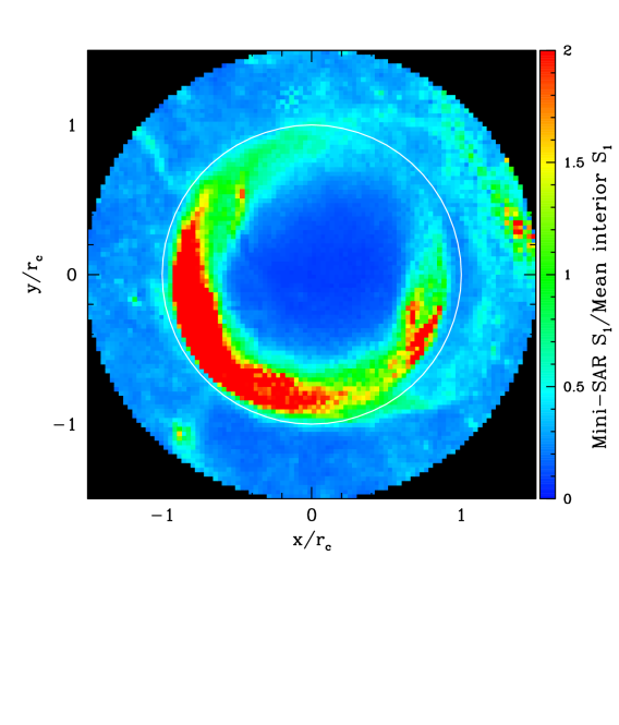
If the anomalously high interior CPR measurements in polar craters were the result of significant deposits of water ice, then one might expect to see a variation of CPR with the position within the crater, reflecting varying insolation, temperature and hence water ice stability (Vasavada et al., 1999). To enhance the signal-to-noise, all $33$ anomalous craters have been stacked together to produce the Mini-SAR CPR map shown in Figure 2. The stacking process involves dividing each pixel’s CPR by the mean crater interior CPR and the distance from the centre is expressed as a fraction of the distance to the crater’s edge. The map for each crater is rotated to have the north pole at the top, and the final stacked map is the mean of these processed crater maps. It is apparent from the figure that the highest CPR is typically on the poleward side of the crater, with a distinctive horseshoe pattern of higher CPR around the crater walls.

Stacking the same $33$ anomalous craters together using the Mini-RF mosaic gives rise to the CPR map in Figure 3. Once again a horseshoe-shaped high CPR region is seen, only in a different part of the stacked crater. Given that the lunar surface will not have changed significantly during the period between Mini-SAR and Mini-RF data collection, it can be inferred that this difference reflects a change in the viewing geometry, as anticipated by the model of Fa et al. (2011) (see their figure 13).

This conclusion is strengthened by the corresponding stacked maps of the returned power shown in Figures 4 and 5, which are determined from the $S_{1}$ mosaics. Higher returned power suggests the transmitted radiation is nearer to normal incidence on the surface. Consequently, there will be greater specular reflection and a lower returned CPR. Thus, the highly reflective parts of the stacked returned power maps correspond to the low parts in the CPR maps. When the surface is viewed at larger angles of incidence, the multiply scattered radiation becomes increasingly important and the returned CPR increases while the returned power decreases. The stacked crater maps shown in these figures all have north to the top, but the radar look direction does not always have the same bearing because the side-facing detector will change its look direction near to the pole. In addition to having different look directions for the different craters contributing to the stacked map, the incidence angle in any given pixel will vary between craters as they have a variety of diameter-to-depth ratios. Consequently, these stacked maps are for illustrative purposes only, and all subsequent radar results treat the craters individually, using a look direction inferred by determining the position of the maximum reflected power in that crater’s $S_{1}$ map.

From these figures, it is clear that the largest factor affecting the CPR maps of these polar craters is the angle of incidence of the observations. As the Mini-RF mosaic includes both left and right-looking measurements it will not be possible to infer an appropriate, reliable single crater look direction from the mosaic, so attention will now be focussed onto the Mini-SAR data.

3.2 Slopes and parallax

Given that the angle of incidence is a complicating, and for the purposes of learning about the lunar surface uninteresting, factor driving the CPR distribution within the polar craters, it would be good to remove its effect. While there have been models of how CPR varies with angle of incidence (Thompson et al., 2011; Fa et al., 2011), a more robust approach involves determining the dependence using the data themselves.

Each crater has an $S_{1}$ map with a high spot that should be nearest to normal incidence for the incoming radar. This is defined within a cone of opening angle $20^{\circ}$ from the centre of the crater, and is used to define the azimuthal look direction of the detector appropriate to this particular crater. In combination with the nadir angle of the detector, this provides a vector for the incoming radiation. Finite differencing methods applied to the LOLA DEM provide a local surface normal. The scalar product of these unit vectors yields the cosine of the angle of incidence for each pixel in each of the craters being considered. In this way, each pixel CPR can be mapped to a corresponding angle of incidence.

Figure 2: The stacked relative CPR map for the 33 anomalous craters. Each crater map is divided by the mean pixel CPR interior to the crater and rotated to have north at the top before they are stacked together. The white circle represents the edge of the craters contributing to the average.

Figure 3: The stack of the 33 anomalous crater relative CPR maps using the LRO Mini-RF unrectified mosaic.

Figure 4: The stacked relative returned power, represented by the first element of the Stokes vector, $S_{1}$, for observations of the 33 anomalous craters made by Mini-SAR. All craters are aligned so that north points to the top of the image before stacking.

Figure 5: The equivalent of Fig. 4 for the LRO Mini-RF $S_{1}$ mosaic.

Figure 6: The variation of median CPR as a function of angle of incidence between the incident radar and the surface normal for the 33 anomalous craters. The light black lines show the individual crater median pixel CPR curves, and the heavy black line is the median of these values. Error bars show an estimate of the statistical uncertainty on the inferred median based on the 16th and 84th percentiles of the distribution of CPR values from the individual craters at each angle of incidence and the assumption that this distribution is Gaussian. The heavy green line is the median over all craters for the crater exterior out to $1.5r_{\rm c}$. Positions have been rectified to account for the parallax prior to determining into which radial range they fall. The red line shows a straight line fit to the median interior CPR relation.

One final, but crucial, complication is to determine to which bit of the surface does an unrectified Mini-SAR mosaic pixel correspond. The effect of parallax in radar range measurements distorts the inferred pixel position because the mapping of return signal time to distance should account for variations in the height of the surface being mapped (Campbell, 2002). As the Mini-SAR crater positions have been individually chosen such that the crater rims appear to line up correctly (something that the stacked CPR and $S_{1}$ mosaics imply has been done reasonably well), the mean altitude of the crater rim is set as the reference height. All other points within $1.5r_{\rm c}$ of the crater centre are then shifted a distance $p$ away from the detector in the range direction using

$$\Delta h=p\tan\alpha,$$ (1)

where $\Delta h$ represents the change in height, at the shifted position, relative to the reference height, $p$ is the parallax, and $\alpha$ is the angle of incidence of the radar (see section 4.11 in Campbell, 2002). An iterative procedure is necessary because the parallax displacements depend upon the topography at to-be-determined positions in the DEM. This shift moves unrectified pixels within the crater having $\Delta h<0$ to positions that are nearer to the detector (i.e. $p<0$). As a consequence, equally spaced pixels in the distorted, unrectified map preferentially sample the near crater wall at higher angles of incidence.

Having determined which part of the LOLA DEM should be matched to each pixel in the vicinities of the craters being considered, the dependence of pixel CPR on the angle of incidence can be determined. Figure 6 shows the median dependence of the pixel values for each of the $33$ anomalous north pole craters being considered here. The median of these curves is shown with the bold black line, which can be well described by the linear fit

$$CPR(\theta)=0.27+0.68(\theta/90^{\circ})$$ (2)

where $\theta$ represents the angle of incidence in degrees. The crater interior shows a strong trend of increasing CPR with increasing angle of incidence, although the individual crater values have a non-negligible scatter about this median relation. A bold green line traces the median dependence for the $33$ crater exterior regions out to $1.5r_{\rm c}$, and clearly shows lower CPR values for intermediate angles of incidence than are typical inside these craters. While the exterior CPR does become more similar to the interior crater values at high and low angles of incidence, it is possible that this is a consequence of inaccuracies in defining the crater edges in the Mini-SAR mosaic.

This measurement of the variation of CPR with angle of incidence could contain dependencies on hidden surface properties that have not been considered, but it serves as a useful starting point for constructing a simple model with which to investigate just how important the rectification process is. A model crater was created with diameter $2r_{\rm c}=6$ km, and a diameter-to-depth ratio of $5.5$, typical of the anomalous polar craters considered here. The radial height profile, $a(x)$, with $x=r/r_{\rm c}$ being the radius in terms of the crater radius, was defined via $y(x)=a(x)/r_{\rm c}$, where

$$y(x)=\left\{\begin{array}[]{ll}y_{0}+\eta x^{2}&{\rm if}~{}x\leq x_{1},\\ y_{1}+y_{1}^{\prime}(x-x_{1})&{\rm if}~{}x_{1}\leq x\leq x_{2},\\ y_{2}+\beta[(x_{2}-1)^{2}-(x-1)^{2}]&{\rm if}~{}x_{2}\leq x\leq x_{3},\\ y_{3}+\gamma[(x-x_{4})^{2}-(x_{3}-x_{4})^{2}]&{\rm if}~{}x_{3}\leq x\leq x_{4},\\ y_{4}&{\rm if}~{}x_{4}\leq x.\end{array}\right.$$ (3)

$y_{0}$ represents the central depth divided by the crater radius, which is just twice the reciprocal of the diameter-to-depth ratio, while $y_{n}$ for $n>0$ is the value of $y$ evaluated at $x_{n}$. $y_{1}^{\prime}$ denotes d$y/$d$x$ evaluated at $x_{1}$. With the outer boundary condition set as $y_{4}=-0.04$ at $x_{4}=1.5$ and the two inner curvatures chosen to be $\eta=1$ and $\beta=2$, the requirements that the function is continuous and differentiable sets the remaining constants via

$$x_{1} = \frac{1-\sqrt{1-\frac{y_{0}}{\eta}(1+\eta/\beta)}}{1+\eta/\beta}$$ (4)

$$x_{2} = 1-\frac{\eta}{\beta}x_{1}$$ (5)

$$x_{3} = 1-\frac{y_{4}}{\beta(x_{4}-1)}$$ (6)

$$\gamma = \frac{\beta(x_{3}-1)}{x_{4}-x_{3}}.$$ (7)

This cross-section for the model crater is shown in Figure 17 and has a maximum smooth slope for the crater wall of tan${}^{-1}y_{1}^{\prime}\approx 23^{\circ}$. A regular $75$ m grid of pixels was created out to $x_{4}=1.5$ from the crater centre. Assuming that these pixels were unrectified, the corresponding rectified positions in the crater were calculated, the angles of incidence to the nominal detector with a nadir angle of $33^{\circ}$ were inferred and CPR values were assigned according to equation (2).

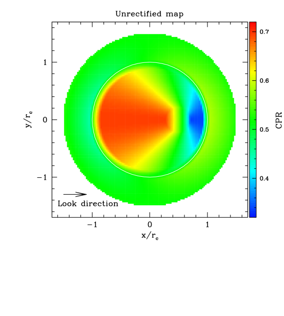
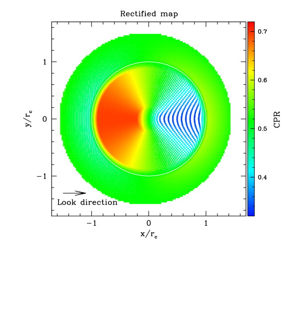
The resulting unrectified CPR mosaic is shown in Figure 7 from which it can be seen that the high CPR values associated with the near wall, viewed at large angles of incidence, occupy a significantly larger fraction of the crater interior pixels than the more nearly normal incidence parts of the far wall. Figure 8 shows the same pixels shifted to the parts of the crater that they actually sample. With the effect of parallax removed from the map, it becomes apparent just how the pixels are biased to measure the CPR of the near wall of the crater. Even with $75$ m unrectified resolution of a $6$ km diameter crater, there are significant parts of the far wall that are completely unsampled.

The impact of this uneven sampling of the crater on the probability distribution of pixel CPR values is shown in Figure 9. Dashed red and green lines show how the interior and exterior pixel CPR distributions can look significantly different, despite both being drawn from an identical relation for CPR as a function of angle of incidence. The peak of the distribution shifts from a CPR of $\sim 0.5$ to $\sim 0.7$, as a result only of the bias caused by using a mosaic uncorrected for the effect of parallax and the dependence of CPR on angle of incidence. These pixel CPR distributions are much more sharply peaked than those in Figure 1 that were measured for real craters using the Mini-SAR mosaic. One way in which the distribution would be broadened would be if there were significant statistical uncertainties on the measurements. The solid lines in Figure 9 show that including a $40\%$ scatter in the assumed CPR at any particular angle of incidence produces distributions that look not unlike those from a few of the anomalous craters.

Figure 7: An unrectified CPR mosaic of a model crater with $r_{\rm c}=3$km, a diameter-to-depth ratio of $5.5$ and a rim height of $0.04r_{\rm c}$. The model SAR is looking from the left with a look angle of $33^{\circ}$ and the mosaic has $75$m square pixels.

Figure 8: The rectified version of Fig. 7, with each coloured point showing the true position within the crater that it samples. White regions show parts of the crater into which none of the unrectified mosaic pixels are mapped when the parallax correction moves pixels beneath the crater rim toward the detector. The colour relates directly to the angle of incidence at which the surface is viewed through equation (2).

Figure 9: The distribution of pixel CPR values for the interior (red) and exterior (green) of the model crater. Dashed lines show results when no scatter is added in the model CPR value at a given angle of incidence, whereas the solid lines show the effect of including a $40$% $1\sigma$ Gaussian scatter around the median value.

Figure 10: The variation of median CPR as a function of angle of incidence between the incident radar and the surface normal for the 33 anomalous craters. Values show the median of the individual crater values that contribute to each increment of incidence angle. Error bars show an estimate of the statistical uncertainty on the inferred median based on the 16th and 84th percentiles of the distribution of CPR values from the individual craters at each angle of incidence and the assumption that this distribution is Gaussian. The different colours represent different radial ranges of pixels. Positions have been rectified to account for the parallax prior to determining into which radial range they fall.

Figure 11: The equivalent of Fig. 10 for the 9 fresh craters. Wider radial ranges are used to suppress statistical noise in the median CPR estimates.

Is it reasonable that such large observational uncertainties exist? This can be indirectly addressed by considering the variation in CPR between adjacent pixels in the Mini-SAR mosaic. The root mean square fractional difference in CPR varies only slightly across the whole polar region, and typically has a value of $25-30\%$ in the vicinity of the craters studied here. This represents an upper limit on the size of the statistical uncertainties in the mosaic CPR values, because some of these variations on small scales are presumably the result of varying surface properties. Thus, it can be safely concluded that observational uncertainties in conjunction with slopes and the bias introduced by parallax are not sufficient to explain the measurements. This implies that there must be some additional process responsible for changing the CPR in a systematic way and that the interior surfaces of these polar anomalous craters are typically different from their exteriors in more complicated ways than merely having steeper slopes.

3.3 The radial variation of CPR

Having determined that the angle of incidence is not solely responsible for the differences between anomalous crater interiors and exteriors, the challenge shifts to trying to determine what other factors are affecting the CPR. Figure 10 shows how the median pixel CPR varies with angle of incidence for different radial ranges both inside and outside the anomalous craters. The pixels are placed into the different radial bins based on their rectified positions within the crater. For all different radial ranges the shape of the median CPR variation with angle of incidence is similar. Only the amplitude changes with radius. The central region of the typical crater has CPR values that are indistinguishable from those of pixels in the crater exterior with $1.2<r/r_{\rm c}<1.5$. Out to $r/r_{\rm c}\sim 0.8$, the CPR at a given angle of incidence increases systematically with increasing radius. Inaccuracies in determining the precise crater locations may scramble any trends at radii around $r_{\rm c}$, but there is a sharper drop in the CPR outside the crater edge than is seen inside the crater. No difference is seen in the results shown in Figure 10 when the anomalous crater sample is split in half either by crater radius or latitude. The increased CPR at any given angle of incidence seems to increase with increasing local slope. At radii satisfying $0.5\mathrel{\hbox{\hbox to0.0pt{\hbox{\lower 4.0pt\hbox{$\sim$}}\hss}\hbox{$<$}}}r/r_{\rm c}\mathrel{\hbox{\hbox to0.0pt{\hbox{\lower 4.0pt\hbox{$\sim$}}\hss}\hbox{$<$}}}1$, where the CPR is largest for a given angle of incidence, the azimuthally-averaged slopes are typically $\sim 25^{\circ}$. However, the inaccuracy in the alignment of CPR and DEM maps and the relatively poor spatial resolution preclude a more detailed comparison of CPR with local slope at present.

The corresponding results for the $9$ fresh craters are shown in Figure 11. Wider bins in radius are used to prevent the results becoming too noisy given the relatively small number of fresh craters. The variation of CPR with angle of incidence is much weaker than for the anomalous craters. Also, the radial variation, while qualitatively similar to that seen for the anomalous craters, is less pronounced. This is consistent with what one might expect from a surface containing a uniform scattering of blocky ejecta behaving like corner reflectors.

Maps of the variation of CPR relative to the typical value at each incidence angle in each crater are shown in Figure 12. Although the maps are quite heterogeneous, the relatively low CPR values tend to be either in the crater centres or on the far wall as viewed by the detector. Arrows show the direction in which each crater is viewed, as determined from the high spots in the individual crater $S_{1}$ maps. Relatively high CPR values tend to be concentrated onto the crater walls. The median CPR values as a function of incidence angle are determined from rectified pixels satisfying $r/r_{\rm c}<0.8$. This is done to prevent errors arising from misalignments between the Mini-SAR mosaic and the LOLA DEM. Near to the crater rim, the slopes change rapidly, such that any misalignments between data sets would lead to pixels being assigned very wrong incidence angles, biasing the inferred CPR as a function of incidence angle. This effect may be behind the slightly non-monotonic behaviour noted in Figure 10 for the radial bins adjacent to the rim.

Figure 13 is included to help the interpretation of the relative CPR maps in Figure 12. It shows how the angle of incidence varies with position within the model crater used in Section 3.2, and is effectively just a rescaled version of Figure 8. The comparison of local CPR with that at comparable angles of incidence, given in Figure 12 within each crater, is showing along a line of constant colour in Figure 13, with the orientation set by the azimuthal look direction, where are the higher and lower values of CPR.

Figure 12: Maps of Mini-SAR CPR/median CPR at that incidence angle for each of the 42 craters. The craters are ordered as in Figure 1 and the pixels are plotted at their rectified locations, with north to the top. Median CPR as a function of incidence angle is calculated for each of the craters individually, using only the pixels with rectified radii having $r/r_{\rm c}<0.8$. Black arrows show the azimuthal look direction inferred from the $S_{1}$ mosaic for each crater.

Figure 13: The distribution of incidence angle for the model crater considered in Section 3.2. This shows which parts of a typical crater are viewed at the same angle of incidence, and represents a remapped version of Fig. 8. The detector is looking along the $+x$ direction at the model crater, as shown by the black arrow.

4 Implications for the detection of water ice

The results in the previous section showed that high CPR regions within polar anomalous craters, once angle of incidence effects are removed to the extent that is possible with the data sets being used here, tend to be found on the steep crater walls. This finding matches that of Thomson et al. (2012) from their detailed study of Shackleton crater. Figure 14 shows the stacked map of the maximum temperature, $T_{\rm max}$, relative to the mean maximum temperature within each crater, inferred from Diviner measurements for the $33$ anomalous craters. For all craters, the largest interior $T_{\rm max}$ values exceed $290$K and are found on the equator-facing walls, where direct sunlight can occasionally be seen. The stacked pole-facing slope and crater floor have the lowest maximum temperatures, typically $70$K but ranging from $30-130$K, because they only ever receive reflected sunlight. Given that surficial water ice should be stable against sublimation for temperatures beneath $\sim 100$K, one might well expect any water ice to be located in these relatively cold regions within the craters. This pattern of maximum temperatures is similar to that seen in the average temperatures, and neither of them reflect the variation of CPR, as might be expected if significant deposits of water ice were responsible for the elevated interior CPRs in the anomalous polar craters.

It is possible that water ice could be insulated by a layer of mantling regolith, in which case the CPR variations within anomalous craters might not be expected to reflect those in the temperature. Perhaps the central regions of craters are covered by too much regolith for the radar to see underlying water ice. In contrast, the steep crater sides should not be covered by deep regolith. However, in these regions, the CPR variations still do not reflect the variations in temperature determined using Diviner data.

Figure 14: The stacked Diviner-inferred pixel $T_{\rm max}$ relative to the mean within each crater for the 33 anomalous craters. North is upwards, so the relatively cold part of the average crater is pole-facing.

Figure 15: The variation of diameter-to-depth ratio ($D/d$) with crater diameter for the 33 anomalous craters (blue filled circles), 9 fresh craters (red open circles) and 154 topographically selected, isolated polar craters (black crosses). The black line represents the variation with diameter of the median of the black points, and the green line traces the relation given by Pike (1974) for fresh lunar craters.

Using the set of $154$ topographically selected polar craters described in the Appendix, one can look at the diameter-to-depth ratios of the fresh and anomalous craters relative to a set that have been found without reference to their CPR properties. The mean diameter-to-depth ratios of the fresh and anomalous craters are $D/d\sim 5.0$ and $5.9$ respectively. Increasing $D/d$ would be expected as craters age, because the depths decrease over time while the diameters change little. These measurements are therefore consistent with the picture of the anomalous craters being older than the fresh ones. However, the topographically selected craters have even larger $D/d$ values, with a mean of $\sim 7.0$. Could these differences be driven by the crater diameter-to-depth ratio varying with crater size? Figure 15 shows the different crater sets as a function of crater diameter. The solid black line represents the median $D/d$ for the topographically selected craters binned into three different diameter ranges, whereas the green line shows the relation found by Pike (1974) for a set of fresh lunar craters. It is clear that the anomalous craters typically have lower diameter-to-depth ratios than the set of polar craters selected only on topography. Under the assumption that $D/d$ is a proxy for crater age, one therefore infers that the anomalous craters, while older than the fresh ones, are still less mature than typical craters in the north polar region. This is again suggestive that the effects of micrometeorite bombardment on the steep crater walls have not yet acted to remove all of the rocks or roughness that give rise to high CPR values.

If micrometeoritic bombardment is isotropic and the blocky debris from the crater forming impacts is weathered away at similar rates inside and outside polar craters, then these results imply that processes are preferentially acting on the steep slopes to refresh the near-surface roughness to which the CPR is sensitive. This picture is consistent with the findings of Bandfield et al. (2011), who use the thermal inertia determined from Diviner measurements to infer rock abundances and regolith thicknesses. They find extra rockiness on steep crater walls relative to crater floors and crater exteriors, which is in qualitative agreement with what is inferred in this study. Similarly, Fa and Cai (2013) use LROC images to show higher rock abundance interior to craters relative to their exteriors. Furthermore, they find this extra rockiness correlates with the difference between interior and exterior CPR values, as measured by Mini-RF. Both the Diviner and LROC rock abundances refer to objects that are at least $1-2$ m in size, which is $\sim 10$ times the S-band radar wavelength. While there is no guarantee that rockiness on these relatively large scales implies roughness on scales more comparable with the radar wavelength, the modelling of Fa and Cai (2013) suggests that the larger rocks can nevertheless provide a significant CPR enhancement through dihedral reflections.

If the anomalous craters do have high CPR as a result of differential weathering of roughness, then the finding reported by Spudis et al. (2013), that the number density of anomalous craters at the poles greatly exceeds that at lower latitudes, remains to be explained. This apparent dependence on temperature is difficult to reconcile with the indifference to local temperature of the CPR distribution within anomalous polar craters. One would really like to start from the topographically-selected crater sample and study the variation of CPR with crater morphology, rather than starting from craters that have a particular CPR distribution, as was done here and in previous work. Looking only at CPR-selected craters can lead to a misleading impression of the population of craters as a whole. An orthorectified CPR mosaic, already tied to the LOLA DEM, would be necessary to avoid topographically-selected craters being ejected from the sample if their CPR was insufficiently distinct for them to be detected via their CPR, which has occurred in this study, as described in Section 2.4.

5 Conclusions

The distribution of pixel CPR values inside and outside fresh craters is largely independent of the angle of incidence with which the lunar surface is viewed. In contrast, for anomalous craters the angle of incidence has a large impact on the CPR maps that result. In these cases, counting pixels in SAR mosaics that have not been rectified for the effect of parallax has the effect of biasing the crater interior CPR pixel distribution to be dominated by observations of the near wall, viewed at larger incidence angle. Consequently, the mean interior crater CPR measured from an unrectified Mini-SAR map would exceed that for the crater exterior even when the interior and exterior surfaces have identical radar reflectivities (see Figure 9).

The typical variation of CPR with angle of incidence was measured within the anomalous craters and used to make a model to quantify how using unrectified mosaics will bias the distribution of pixel CPRs inside the crater relative to that from just outside. While this effect alone creates a sufficient change in the mean pixel CPR to explain some of the anomalous craters, the additional scatter required to recover the observed CPR distributions exceeds the statistical uncertainties on the measurements. Therefore, the CPR is also significantly affected by variations in the surface properties.

An additional variation with distance from the crater centre has also been discovered, with the crater centre having CPR values like those of the crater exterior, while larger CPR values at any given incidence angle are found on the steeper parts of the crater walls. It is argued that this variation of CPR with local slope, rather than local temperature, suggests that it results from a variation in the extent to which roughness is visible to the incident radar. Steeper walls near the angle of repose may be less able to sustain enough fine regolith to prevent the radar from seeing the rougher rocks underneath or it could just be that ongoing weathering produces more surface rocks or roughness on steeper slopes.

This argument is supported by the fact that anomalous craters, while having larger diameter-to-depth ratios than fresh ones, are typically steeper-sided than craters determined using a crater-finding algorithm applied to the LOLA DEM. Assuming that the diameter-to-depth represents a proxy for crater age, the anomalous craters are of intermediate age. If surface roughness refreshed by mass-wasting on steep slopes were responsible for the high CPR, then one would expect anomalous craters to be of intermediate age, because fresh craters have high CPR both inside and outside, whereas old craters do not retain sufficiently steep sides for mass-wasting to continue to promote sufficient surface roughness to cause high CPR. Thus, the surface roughness explanation appears to pass this test.

Future analyses of the lunar SAR data should use properly controlled and rectified CPR mosaics that are tied to the LOLA global DEM and take into account explicitly the dependence of CPR on angle of incidence. The model of Fa et al. (2011), while not including multiple scattering and the CBOE, suggests that radar data will not be able to distinguish between regolith with and without a few wt% WEH, which is the level that the LCROSS and LPNS results imply is the likely concentration. There is strong circumstantial evidence that the extractable information from the lunar SAR data will pertain to surface or near-surface roughness rather than water ice. This should provide fertile ground in conjunction with Diviner and LROC data sets to learn about surface weathering as a function of local slope and composition (Bell et al., 2012).

References

Appendix A Crater-finding algorithm

The list of craters produced by Head et al. (2010) from the LOLA topographical data consists of 5185 craters with radii of at least $10$ km distributed over the entire lunar surface. Salamunićcar et al. (2012) supplemented this with additional craters found using a predominantly automated detection algorithm that was based on the LOLA DEM. Their crater catalogue contained 60645 objects and is the most complete to radii of $4$ km. For the purpose of this study, even smaller craters in the vicinity of the lunar north pole are of interest, and the desire is to produce craters with representative diameter-to-depth ratios. Thus, an algorithm has been developed to find simple craters with radii in the range $2\leq r_{\rm c}/{\rm km}\leq 10$ using the LOLA north polar stereographic digital elevation map.

The crater-finding algorithm consists of two main stages. First, by placing ‘water’ on the surface and letting it drain downhill to create puddles, a set of potential crater centres are found. The amount of water in each puddle reflects the area from which it came and hence provides an estimate of the radius of the potential crater. Secondly, in the vicinity of each potential crater, the Laplacian of the topography is filtered to search for circularly symmetric patterns with a concave centre surrounded by a convex rim. The details of these two parts of the algorithm are described in the following subsections.

A.1 Finding crater candidates

Candidates for crater centres are found using a hydrological algorithm that is a simplified version of those described by O’Callaghan and Mark (1984) and Freeman (1991). A smoothed version of the LOLA polar stereographic $80$ m DEM is used. The smoothing suppresses small scale depressions that might otherwise prevent ‘water’ from draining further into larger depressions. It also removes candidate tiny craters that might be within other craters, which would consequently fail the isolation criterion described in the next section and be jettisoned from the sample. A single smoothing entails replacing each altitude with a value that is $1/4$ of the original value plus $1/8$ of each of the values in the $4$ adjacent pixels, plus $1/16$ times the values in the diagonally adjacent pixels. Given that craters in the radius range $2-10$ km are being considered here, 3 smoothings of the DEM are used.

An amount of ‘water’ proportional to the pixel area is placed into each pixel in the smoothed digital elevation map and this is allowed to run downhill using the following iterative method. Each pixel with none of its 8 neighbours being higher and containing water, distributes its water to neighbouring pixels that are lower than it. The water is distributed to the $N$ lower neighbouring pixels in proportion to the gradient in their direction. Thus, the fraction of water sent to the $i$th lower neighbour is given by

$$f_{i}=\frac{|\underline{\nabla}_{i}|}{\sum_{j=1}^{N}|\underline{\nabla}_{j}|},$$ (8)

where $\underline{\nabla}_{i}$ represents the gradient in the direction of the $i$th neighbour. This draining is repeated until no pixels with lower neighbours contain any water, at which point the set of ‘wet’ pixels defines the centres of crater candidates, with the amount of water providing an estimate of the potential crater radius under the assumption that it came from a circular patch of the surface.

A.2 Confirming craters

For the purpose of this study, there is no need to have a complete sample of craters, merely one that is representative of the diameter-to-depth ratios of craters as a whole. Thus, for simplicity, only isolated crater candidates are retained for further consideration. Isolation is defined as having no other crater candidate within one candidate crater radius from the candidate crater centre. This yields a set of $\sim 68000$ candidate isolated craters of all radii at ${\rm latitude}>80^{\circ}$. These candidates are then filtered to refine the centres and radii and determine a statistic related to how much they match a simple crater in their topographic profile.

The Laplacian of the DEM in the vicinity of each of these potential craters is filtered using a compensated filter of the form

$$w(r)=\left\{\begin{array}[]{ll}N_{\rm ring}/N_{\rm cen}&{\rm if~{}~{}~{}}r<0.6r_{\rm c,test},\\ -1&{\rm if~{}~{}}|r-r_{\rm c,test}|\leq 40{\rm m,}\\ 0&{\rm otherwise,}\end{array}\right.$$ (9)

where $r_{\rm c,test}$ is the crater radius being tested, $N_{\rm cen}$ is the number of $80$ m pixel centres lying within a disc of radius $0.6r_{\rm c,test}$ and $N_{\rm ring}$ is the number of pixel centres within an annulus one pixel wide having mean radius equal to $r_{\rm c,test}$. Crater radii are tested in the range $0.5-1.5$ times the value inferred from the amount of water gathered by each candidate. This filter picks out regions that have a concave disc of surface surrounded by a convex rim-like structure. The pixels within which the maximum filtered Laplacian values are found for each tested crater radius provide the most likely crater centres for those test radii.

To determine which tested radius produces the best overall match, a significance of the value of the filtered Laplacian is defined. Applying the filter to a random part of the Laplacian map inferred from the DEM would give rise to a distribution of filter values. This can be treated as a random walk with a step size of the rms Laplacian weighted by the rms step size of the filter. Using this to normalise the filtered Laplacian values around the candidate crater centre gives a significance for each candidate crater. This value is used to determine the best test radius. Each candidate with a significance, $S$, (of the filtered Laplacian relative to that expected from a random walk) of at least $S_{\rm min}=15$ is deemed to be a detected crater.

A.3 The set of polar craters

The algorithm described above yields $154$ craters with latitude greater than $80^{\circ}$. Table A1 contains a list of the centres and radii of these north polar, isolated craters, and Figure 16 shows their distribution with diameter. Figure 15 plots the dependence of the crater diameter-to-depth ratios on diameter, illustrating how these topographically selected craters typically have shallower profiles than either the fresh or anomalous craters studied by Spudis et al. (2010).

The choice of $S_{\rm min}$ feeds into the inferred diameter-to-depth ratio of the resulting crater catalogue, because deeper craters better match the filter shape than shallower ones. Thus, increasing $S_{\rm min}$ from $15$ to $20$ decreases the number of craters from $154$ to $108$, and the diameter-to-depth ratio from $7.0$ to $6.3$. However, the lower threshold of $S_{\rm min}=15$ still produces a set of azimuthally symmetric depressions with convex rims that are crater-like. Figure 17 shows the azimuthally-averaged height profiles, scaled by crater radius, of all $154$ craters with $S>15$. The diversity of depths reflects the range of diameter-to-depth values for the selected craters, and it is apparent that each of the craters possesses both a central depression and a convex rim.

Figure 16: The probability distributions of the crater diameters for the three different sets of craters: $154$ topographically selected (black), $9$ fresh (red) and $33$ anomalous (blue). Coloured arrows show the mean diameters in each sample.

Figure 17: The azimuthally averaged height profiles, scaled by crater radius, for the $154$ topographically selected craters. Each radius is rescaled by the crater radius, $r_{\rm c}$, whereas the scaled height is plotted relative to the value at $r/r_{\rm c}=1.1$. The bold red line shows the profile for the model crater used in Section 3.2, offset vertically by $0.1$ for clarity.

Table 2: Radii and locations for the $154$ topographically selected isolated craters. Longitudes and latitudes are given in degrees.

Crater #	$r_{\rm c}$/km	(lat,lon)	Crater #	$r_{\rm c}$/km	(lat,lon)	Crater #	$r_{\rm c}$/km	(lat,lon)	Crater #	$r_{\rm c}$/km	(lat,lon)
1	2.4	80.01, -21.4	2	2.7	80.01, 31.8	3	2.1	81.12, -21.4	4	2.9	81.35, 19.0
5	4.9	81.65, -23.9	6	2.6	82.26, 11.7	7	2.4	81.84, 28.2	8	2.3	81.49, -32.9
9	2.7	81.85, 29.2	10	2.1	81.83, -31.1	11	2.1	80.07, -46.6	12	2.2	81.98, -34.3
13	3.9	82.65, 26.7	14	2.0	83.29, -13.7	15	2.7	82.07, -37.1	16	2.5	83.06, 24.5
17	8.7	80.26, -50.1	18	2.0	82.49, -34.2	19	2.8	83.87, -7.4	20	5.3	83.76, -13.9
21	2.5	82.68, -37.4	22	2.4	84.12, 15.7	23	3.6	80.80, 53.7	24	2.0	84.14, -21.7
25	2.2	84.18, -20.4	26	2.3	84.64, -6.2	27	2.3	80.01, 61.6	28	2.0	81.87, -56.8
29	2.1	81.43, 59.7	30	4.3	80.16, -66.1	31	3.7	80.32, 65.9	32	3.7	85.78, 25.2
33	2.9	85.91, -27.7	34	2.1	83.64, -55.7	35	3.5	80.46, -68.7	36	2.8	81.19, -68.2
37	4.8	83.89, -57.4	38	2.3	84.88, -50.7	39	2.6	83.94, -59.3	40	2.8	85.75, 43.6
41	2.2	81.40, 69.7	42	2.1	84.57, -56.7	43	2.4	85.30, -52.3	44	2.3	81.08, 71.8
45	5.4	86.99, 28.6	46	2.3	85.79, 54.0	47	3.5	81.85, 72.8	48	3.2	87.12, -33.4
49	2.0	86.89, -45.6	50	2.0	87.52, -29.3	51	2.5	87.69, 30.8	52	2.6	83.91, 72.4
53	2.1	84.51, -70.6	54	2.7	81.47, -77.8	55	2.4	82.80, 75.5	56	2.9	87.97, 29.9
57	2.7	86.64, 58.5	58	2.3	88.08, -27.8	59	2.6	84.90, -71.5	60	2.1	88.22, -26.0
61	3.4	88.26, 25.2	62	3.4	81.50, -79.8	63	2.7	88.08, 39.9	64	3.1	87.92, 57.1
65	3.1	87.66, 63.2	66	2.4	85.59, 76.9	67	4.7	87.36, 68.0	68	2.2	86.01, 76.0
69	2.5	86.65, 73.7	70	3.2	85.75, 78.1	71	2.1	87.81, -66.8	72	2.5	88.75, 47.0
73	2.3	82.66, -83.6	74	3.2	81.56, -84.6	75	3.3	88.19, 63.4	76	2.6	85.56, 79.5
77	2.6	88.96, -45.1	78	3.9	88.05, 68.4	79	2.8	82.71, -87.1	80	2.9	81.22, 88.4
81	2.4	83.32, 88.2	82	4.1	87.13, -86.3	83	2.6	85.97, 88.1	84	2.0	89.64, -108.8
85	2.6	86.27, 94.0	86	2.0	86.89, 96.4	87	2.3	83.65, 93.7	88	2.0	88.17, 112.0
89	2.0	87.69, 107.9	90	2.4	87.83, 113.0	91	2.5	85.43, 101.1	92	3.4	87.41, 110.0
93	2.7	80.43, -99.5	94	2.0	88.41, -177.9	95	2.1	84.87, -109.0	96	2.1	81.87, -102.2
97	2.1	82.54, 105.1	98	2.4	83.09, -106.4	99	2.1	87.24, 135.7	100	2.5	83.74, -108.7
101	3.6	83.35, -108.3	102	2.5	84.00, -110.7	103	2.1	81.40, -104.7	104	2.9	84.55, -114.5
105	3.9	82.41, 107.5	106	2.0	87.66, 172.3	107	2.5	84.72, -116.9	108	2.2	81.45, 106.2
109	2.4	85.94, -129.2	110	3.1	80.51, 107.7	111	2.1	81.85, 110.8	112	2.4	86.64, 152.8
113	2.2	85.63, -134.4	114	2.4	84.62, 125.5	115	5.4	82.63, 116.0	116	2.0	85.15, 132.9
117	2.3	85.24, 136.3	118	2.4	81.54, -114.6	119	2.6	81.01, 113.5	120	2.0	84.44, -130.7
121	2.4	84.00, -127.4	122	3.2	84.49, -132.4	123	2.2	86.18, -177.6	124	2.2	85.85, -157.1
125	4.4	81.08, 115.8	126	2.0	83.37, 126.1	127	4.1	80.93, -115.6	128	2.2	81.45, 118.2
129	4.0	83.10, 129.9	130	3.2	83.73, -135.3	131	4.0	80.45, -122.7	132	4.1	82.24, -134.2
133	4.3	84.05, -156.4	134	3.3	80.17, -124.6	135	2.3	80.58, 126.4	136	2.6	84.10, -163.4
137	2.1	83.22, 147.8	138	2.9	83.99, 174.0	139	2.1	84.00, -176.2	140	2.3	82.90, 150.9
141	4.6	82.46, 145.7	142	5.3	81.15, 137.7	143	2.3	80.31, -135.4	144	2.3	80.74, 146.0
145	2.3	80.97, -161.1	146	2.1	81.29, 171.3	147	2.1	80.97, -162.7	148	4.3	80.46, -155.1
149	2.7	80.38, -156.1	150	2.6	80.71, 164.1	151	2.1	80.96, 172.6	152	2.9	80.27, 158.6
153	2.8	80.84, 173.3	154	2.1	80.18, 176.4

References

- Bandfield et al. (2011) Bandfield, J. L., Ghent, R. R., Vasavada, A. R., Paige, D. A., Lawrence, S. J., Robinson, M. S., Dec. 2011. Lunar surface rock abundance and regolith fines temperatures derived from LRO Diviner Radiometer data. Journal of Geophysical Research (Planets) 116, E003866.
- Bell et al. (2012) Bell, S. W., Thomson, B. J., Dyar, M. D., Neish, C. D., Cahill, J. T. S., Bussey, D. B. J., Nov. 2012. Dating small fresh lunar craters with Mini-RF radar observations of ejecta blankets. Journal of Geophysical Research (Planets) 117, E004007.
- Butler (1997) Butler, B. J., Aug. 1997. The migration of volatiles on the surfaces of Mercury and the Moon. J. Geophys. Res. 102, 19283–19292.
- Campbell (2002) Campbell, B. A., Mar. 2002. Radar Remote Sensing of Planetary Surfaces.
- Campbell (2012) Campbell, B. A., Jun. 2012. High circular polarization ratios in radar scattering from geologic targets. Journal of Geophysical Research (Planets) 117, 6008.
- Campbell et al. (2006) Campbell, D. B., Campbell, B. A., Carter, L. M., Margot, J.-L., Stacy, N. J. S., Oct. 2006. No evidence for thick deposits of ice at the lunar south pole. Nature 443, 835–837.
- Campbell et al. (1978) Campbell, D. B., Chandler, J. F., Ostro, S. J., Pettengill, G. H., Shapiro, I. I., May 1978. Galilean satellites - 1976 radar results. Icarus34, 254–267.
- Clark (2009) Clark, R. N., Oct. 2009. Detection of Adsorbed Water and Hydroxyl on the Moon. Science 326, 562.
- Colaprete et al. (2010) Colaprete, A., Schultz, P., Heldmann, J., Wooden, D., Shirley, M., Ennico, K., Hermalyn, B., Marshall, W., Ricco, A., Elphic, R. C., Goldstein, D., Summy, D., Bart, G. D., Asphaug, E., Korycansky, D., Landis, D., Sollitt, L., Oct. 2010. Detection of Water in the LCROSS Ejecta Plume. Science 330, 463.
- Crider and Vondrak (2000) Crider, D. H., Vondrak, R. R., Nov. 2000. The solar wind as a possible source of lunar polar hydrogen deposits. J. Geophys. Res. 105, 26773–26782.
- Crider and Vondrak (2003) Crider, D. H., Vondrak, R. R., Jun. 2003. Space weathering of ice layers in lunar cold traps. Advances in Space Research 31, 2293–2298.
- Eke et al. (2009) Eke, V. R., Teodoro, L. F. A., Elphic, R. C., Mar. 2009. The spatial distribution of polar hydrogen deposits on the Moon. Icarus200, 12–18.
- Fa and Cai (2013) Fa, W., Cai, Y., Aug. 2013. Circular polarization ratio characteristics of impact craters from Mini-RF observations and implications for ice detection at the polar regions of the Moon. Journal of Geophysical Research (Planets) 118, 1582–1608.
- Fa et al. (2011) Fa, W., Wieczorek, M. A., Heggy, E., Mar. 2011. Modeling polarimetric radar scattering from the lunar surface: Study on the effect of physical properties of the regolith layer. Journal of Geophysical Research (Planets) 116, 3005.
- Feldman et al. (1998) Feldman, W. C., Maurice, S., Binder, A. B., Barraclough, B. L., Elphic, R. C., Lawrence, D. J., Sep. 1998. Fluxes of Fast and Epithermal Neutrons from Lunar Prospector: Evidence for Water Ice at the Lunar Poles. Science 281, 1496–1500.
- Freeman (1991) Freeman, T., 1991. Calculating catchment area with divergent flow based on a regular grid. Computers and Geosciences 17, 413–422.
- Gladstone et al. (2012) Gladstone, G. R., Retherford, K. D., Egan, A. F., Kaufmann, D. E., Miles, P. F., Parker, J. W., Jan. 2012. Far-ultraviolet reflectance properties of the Moon’s permanently shadowed regions. Journal of Geophysical Research (Planets) 117, E003913.
- Hapke (1990) Hapke, B., Dec. 1990. Coherent backscatter and the radar characteristics of outer planet satellites. Icarus 88, 407–417.
- Harmon et al. (1994) Harmon, J. K., Slade, M. A., Vélez, R. A., Crespo, A., Dryer, M. J., Johnson, J. M., May 1994. Radar mapping of Mercury’s polar anomalies. Nature 369, 213–215.
- Head et al. (2010) Head, J. W., Fassett, C. I., Kadish, S. J., Smith, D. E., Zuber, M. T., Neumann, G. A., Mazarico, E., Sep. 2010. Global Distribution of Large Lunar Craters: Implications for Resurfacing and Impactor Populations. Science 329, 1504.
- Kirk et al. (2013) Kirk, R. L., Becker, T. L., Shinaman, J., Edmundson, K. L., Cook, D., Bussey, D. B. J., Mar. 2013. A Radargrammetric Control Network and Controlled Mini-RF Mosaics of the Moon’s North Pole…at Last! In: Lunar and Planetary Institute Science Conference Abstracts. Vol. 44 of Lunar and Planetary Institute Science Conference Abstracts. p. 2920.
- Lawrence et al. (2006) Lawrence, D. J., Feldman, W. C., Elphic, R. C., Hagerty, J. J., Maurice, S., McKinney, G. W., Prettyman, T. H., Aug. 2006. Improved modeling of Lunar Prospector neutron spectrometer data: Implications for hydrogen deposits at the lunar poles. Journal of Geophysical Research (Planets) 111, E08001.
- Lawrence et al. (2013) Lawrence, D. J., Feldman, W. C., Goldsten, J. O., Maurice, S., Peplowski, P. N., Anderson, B. J., Bazell, D., McNutt, R. L., Nittler, L. R., Prettyman, T. H., Rodgers, D. J., Solomon, S. C., Weider, S. Z., Jan. 2013. Evidence for Water Ice Near Mercury’s North Pole from MESSENGER Neutron Spectrometer Measurements. Science 339, 292.
- Nozette et al. (1996) Nozette, S., Lichtenberg, C. L., Spudis, P., Bonner, R., Ort, W., Malaret, E., Robinson, M., Shoemaker, E. M., Nov. 1996. The Clementine Bistatic Radar Experiment. Science 274, 1495–1498.
- Nozette et al. (2010) Nozette, S., Spudis, P., Bussey, B., Jensen, R., Raney, K., Winters, H., Lichtenberg, C. L., Marinelli, W., Crusan, J., Gates, M., Robinson, M., Jan. 2010. The Lunar Reconnaissance Orbiter Miniature Radio Frequency (Mini-RF) Technology Demonstration. Space Sci. Rev.150, 285–302.
- O’Callaghan and Mark (1984) O’Callaghan, J. F., Mark, D. M., 1984. The extraction of drainage networks from digital elevation data. Computer Vision, Graphics, and Image Processing 28, 323–344.
- Ostro et al. (1992) Ostro, S. J., Campbell, D. B., Simpson, R. A., Hudson, R. S., Chandler, J. F., Rosema, K. D., Shapiro, I. I., Standish, E. M., Winkler, R., Yeomans, D. K., Nov. 1992. Europa, Ganymede, and Callisto - New radar results from Arecibo and Goldstone. J. Geophys. Res. 97, 18227.
- Paige et al. (2010) Paige, D. A., Siegler, M. A., Zhang, J. A., Hayne, P. O., Foote, E. J., Bennett, K. A., Vasavada, A. R., Oct. 2010. Diviner Lunar Radiometer Observations of Cold Traps in the Moon’s South Polar Region. Science 330, 479.
- Pieters et al. (2009) Pieters, C. M., Goswami, J. N., Clark, R. N., Annadurai, M., Boardman, J., Buratti, B., Combe, J.-P., Oct. 2009. Character and Spatial Distribution of OH/H2O on the Surface of the Moon Seen by M3 on Chandrayaan-1. Science 326, 568.
- Pike (1974) Pike, R. J., Nov. 1974. Depth/diameter relations of fresh lunar craters - Revision from spacecraft data. Geophys. Res. Lett. 1, 291–294.
- Raney (2007) Raney, R. K., Nov. 2007. Hybrid-Polarity SAR Architecture. IEEE Transactions on Geoscience and Remote Sensing 45, 3397–3404.
- Salamunićcar et al. (2012) Salamunićcar, G., Lončarić, S., Mazarico, E., Jan. 2012. LU60645GT and MA132843GT catalogues of Lunar and Martian impact craters developed using a Crater Shape-based interpolation crater detection algorithm for topography data. P&SS60, 236–247.
- Simpson and Tyler (1999) Simpson, R. A., Tyler, G. L., Feb. 1999. Reanalysis of Clementine bistatic radar data from the lunar South Pole. J. Geophys. Res. 104, 3845–3862.
- Smith et al. (2010) Smith, D. E., Zuber, M. T., Neumann, G. A., Lemoine, F. G., Mao, D.-d., Smith, J. C., Bartels, A. E., Sep. 2010. Initial observations from the Lunar Orbiter Laser Altimeter (LOLA). Geophys. Res. Lett. 37, 18204.
- Spudis et al. (2010) Spudis, P. D., Bussey, D. B. J., Baloga, S. M., Butler, B. J., Carl, D., Carter, L. M., Chakraborty, M., Mar. 2010. Initial results for the north pole of the Moon from Mini-SAR, Chandrayaan-1 mission. Geophys. Res. Lett. 37, 6204.
- Spudis et al. (2013) Spudis, P. D., Bussey, D. B. J., Baloga, S. M., Cahill, J. T. S., Glaze, L. S., Patterson, G. W., Raney, R. K., Thompson, T. W., Thomson, B. J., Ustinov, E. A., Oct. 2013. Evidence for water ice on the moon: Results for anomalous polar craters from the LRO Mini-RF imaging radar. Journal of Geophysical Research (Planets) 118, 2016–2029.
- Spudis et al. (2009) Spudis, P. D., Bussey, D. B. J., Butler, B., Carter, L., Gillis-Davis, J., Goswami, J., Heggy, E., Kirk, R., Misra, T., Nozette, S., Robinson, M. S., Raney, R. K., Thomson, B., Ustinov, E., Mar. 2009. The Mini-SAR Imaging Radar on the Chandrayaan-1 Mission to the Moon. In: Lunar and Planetary Institute Science Conference Abstracts. Vol. 40 of Lunar and Planetary Institute Science Conference Abstracts. p. 1098.
- Stacy et al. (1997) Stacy, N. J. S., Campbell, D. B., Ford, P. G., 1997. Arecibo radar mapping of the lunar poles: A search for ice deposits. Science 276, 1527–1530.
- Sunshine et al. (2009) Sunshine, J. M., Farnham, T. L., Feaga, L. M., Groussin, O., Merlin, F., Milliken, R. E., A’Hearn, M. F., Oct. 2009. Temporal and Spatial Variability of Lunar Hydration As Observed by the Deep Impact Spacecraft. Science 326, 565.
- Teodoro et al. (2010) Teodoro, L. F. A., Eke, V. R., Elphic, R. C., Jun. 2010. Spatial distribution of lunar polar hydrogen deposits after KAGUYA (SELENE). Geophys. Res. Lett. 37, 12201.
- Thompson et al. (2011) Thompson, T. W., Ustinov, E. A., Heggy, E., Jan. 2011. Modeling radar scattering from icy lunar regoliths at 13 cm and 4 cm wavelengths. Journal of Geophysical Research (Planets) 116, 1006.
- Thomson et al. (2012) Thomson, B. J., Bussey, D. B. J., Neish, C. D., Cahill, J. T. S., Heggy, E., Kirk, R. L., Patterson, G. W., Raney, R. K., Spudis, P. D., Thompson, T. W., Ustinov, E. A., Jul. 2012. An upper limit for ice in Shackleton crater as revealed by LRO Mini-RF orbital radar. Geophys. Res. Lett. 39, 14201.
- Vasavada et al. (1999) Vasavada, A. R., Paige, D. A., Wood, S. E., Oct. 1999. Near-Surface Temperatures on Mercury and the Moon and the Stability of Polar Ice Deposits. Icarus 141, 179–193.
- Watson et al. (1961) Watson, K., Murray, B., Brown, H., May 1961. On the Possible Presence of Ice on the Moon. J. Geophys. Res. 66, 1598–1600.