Nuclear shape coexistence: A study of the even-even Hg isotopes using the interacting boson model with configuration mixing

Abstract

Background:

The Po, Pb, Hg, and Pt region is known for the presence of coexisting structures that correspond to different particle-hole configurations in the Shell Model language or equivalently to nuclear shapes with different deformation.

Purpose:

We intend to study the configuration mixing phenomenon in the Hg isotopes and to understand how different observables are influenced by it.

Method:

We study in detail a long chain of mercury isotopes, ^172-200Hg, using the interacting boson model with configuration mixing. The parameters of the Hamiltonians are fixed through a least square fit to the known energies and absolute B(E2) transition rates of states up to $3$ MeV.

Results:

We obtained the IBM-CM Hamiltonians and we calculate excitation energies, B(E2)’s, quadrupole shape invariants, wave functions, isotopic shifts, and mean field energy surfaces.

Conclusions:

We obtain a fairly good agreement with the experimental data for all the studied observables and we conclude that the Hamiltonian and the states we obtain constitute a good approximation to the Hg isotopes.

I Introduction

The exploration of the many facets of the atomic nucleus over many decades, using a large set of complementary probes, using in particular the electromagnetic (nuclear electric and magnetic transition probabilities and moments, mapping of nuclear charge radii over large series of isotopes) and strong forces, has unambiguously shown the appearance of the essential degrees of freedom. Both, few nucleon properties (near closed shells and doubly-closed shells) as well as collective properties have been discovered bomot75 , most often going hand in hand with the increasing technical possibilities that bring even nuclei far from the region of $\beta$ stability within reach (see in particular Chapter 1 of Rowe and Wood rowe10 ).

A theoretical description of the atomic nucleus, viewed as a system of A nucleons (Z protons and N neutrons) interacting through an in-medium effective nucleon force has reached important progress during the last decades epel09 ; mach11 ; caurier05 ; bender03 . However, it looks like generic characteristics of nuclear excitations stem from the interplay of, on one side, the low multipoles of that interaction that generate nuclear mean-field properties, characterized by a nuclear shell structure and, on the other side, the high multipoles, scattering the interacting nucleons out of their independent particle orbitals, evidenced by the nuclear pairing properties characterized by an energy gap that allows nuclear superfluidity dean03 to appear along long series of isotopes and isotones.

It seems that the balance between these two opposing nuclear force components, i.e., on one side the stabilizing effect of closed shells which prefers nuclei to exhibit a spherical shape, versus a redistribution of protons and/or neutrons in a more deformed shape is at the origin of the appearance of nuclear shape coexistence. By now, nuclear shape coexistence has evolved from the early interpretation of Morinaga morinaga56 , into a phenomenon that appears all through the nuclear landscape, both in light nuclei (near the N $=8,20,28,40$ neutron closed shells) as well as in heavy nuclei (see jul01 ; neyens03 ; blaum13 ; gade08 ; gorgen10 ; bauman12 ; blum13 and hey83 ; wood92 ; heyde11 for an extensive discussion of both the experimental methods and theoretical model approaches over a period of about 3 decades).

Two naturally complementary roads can be taken in order to describe the phenomenon of nuclear shape coexistence. Starting from a nuclear shell-model approach, protons and neutrons are expected to gradually fill the various shells at Z, N $=2,8,20,28,$ … giving rise to a number of double-closed shell nuclei that are the reference points determining shells in which valence nucleons have been allowed to interact through either a phenomenologically fitted effective interaction or a microscopic effective interaction, deduced from many-body theory from realistic NN forces barrett13 ; bogner10 ; cora09 . In view of the large evidence that multi-particle multi-hole excitations are observed, even at a rather low excitation energy, it is important to delineate those regions in the nuclear mass table where conditions are such that shape coexistence may show up. It turns out that it is the balance between the cost to excite such mp-nh excitations at first and the energy gain that results from the enlarged availability of protons and neutrons to interact strongly through the low nuclear multipoles such as to give rise to a “deformed-spherical” inversion or the presence of low-lying competing shape coexisting configurations. With the advent of a strongly increased computing power as well as of the construction of improved algorithms to determine the energy eigenvalues of very big energy matrices, a very large body of calculations mainly along series of isotones at N $=8,20,28,40,$ and, very recently, at N=50 has appeared in the literature. Even the well-known doubly-closed shell nuclei ¹⁶O, ⁴⁰Ca, ⁵⁶Ni, ⁴⁸Ca, … exhibit a number of mp-mh excitations. In these calculations, it is paramount to treat the change in the monopole part of the nuclear field (the changing single-particle energies) as well as the other multipoles originating from the nuclear interaction in a consistent way sorlin08 ; otsuka13 .

In the other approach, the starting point is an effective nuclear force or energy-density functional which are used to derive the optimized single-particle basis in a self-consistent way, making use of Hartree-Fock (HF), or using Hartree-Fock-Bogoliubov (HFB) theory, when also including the strong nucleon pairing forces in both cases constraining the nuclear density distribution to specific values for the quadrupole moments, octupole moments, etc bender03 ; drut10 . In order to confront the results of mean-field studies with the experimental data, one needs to restore the symmetries that are broken in the construction of a HF or HFB reference state. It is necessary therefore to construct states that correspond to a fixed proton (Z) and neutron number (N) as well as good angular momentum J (including K for deformed nuclei). These states then form the starting basis to introduce the dynamical collective correlations beyond the mean-field energy (solving the Hill-Wheeler equations). This gives rise to energy spectra and many other properties such as B(E2) values, quadrupole moments, charge radii and E0 transition rates and can serve as a very good basis to be confronted with the data. Besides the use of various effective forces in the HF (HFB) approach (Skyrme force erler11 , Gogny-force gogny80 ; gogny88 ), a relativistic mean-field approach has been formulated early on by Walecka walecka74 and improved over the years into a microscopic effective-field theory serot86 ; reinhard89 ; serot92 ; ring96 ; niksic11 . It has been shown that the Generator Coordinate Method (GCM) with the Gaussian overlap approximation (GOA) reduces the problem of solving the Hill-Wheeler equations into solving an equivalent collective Bohr Hamiltonian for the full five-dimensional collective model bender03 . This approach has been used frequently with Gogny forces within the framework of both standard constrained Hartree-Fock-Bogoliubov (CHFB) calculations dela10 as well as making use of relativistic mean-field methods niksic11 .

A particularly well-documented example of shape coexistence shows up in the Pb region. From the closed neutron shell (N=126) to the very neutron-deficient nuclei, approaching and even going beyond the N=104 mid-shell nuclei, ample experimental evidence for shape coexisting bands has accumulated for the Pb (Z=82), the Po (Z=84), the Hg (Z=80) and the Pt (Z=78) nuclei jul01 ; hey83 ; wood92 ; heyde11 . Major steps have been taken over a period of more than 3 decades since the early work, disclosing the presence of low-lying 0⁺ states in the ^192-198Pb nuclei duppen84 . The discovery of three shape coexisting configurations in the mid-shell ¹⁸⁶Pb nucleus (at N=104) andrei00 even accelerated the accumulation of new data since 2010. Very recent experimental campaigns have largely extended our knowledge beyond the excitation energies of intruding bands by providing information on nuclear lifetimes dewald03 ; grahn06 ; grahn08 ; grahn09 ; scheck10 , nuclear charge radii dewitte07 ; cocio11 ; seliv13 , 2${}_{1}^{+}$ gyromagnetic factors stuchbery96 ; bian07 , $\alpha$-decay hindrance factors wauters94 ; wauters94a ; richards96 ; uusitalo97 ; duppen00 ; delion95 ; richards97 and, very recently, Coulomb excitation using radioactive beams at REX-ISOLDE (CERN) Isol12 .

An important question is how these shape coexisting structures will evolve when one moves further away from the Z=82 and N=126 closed shells. Whereas the intruder bands are easily singled out for the Pb and Hg nuclei in which the excitation energies display the characteristic parabolic pattern with minimal excitation energy around the N=104 neutron mid-shell nucleus, this structure is not immediate in both the Pt and the Po nuclei.

Theoretical efforts have been carried out over the years, both exploring the mean-field behaviour, even going beyond including the collective dynamics, as well as making use of symmetry-dictated truncated shell-model calculations.

Early calculations started from a deformed Woods-Saxon potential, exploring the nuclear energy surfaces as a function of the quadrupole deformation variables may77 ; bengt87 ; bengt89 ; naza93 and showed a consistent picture pointing to the presence of oblate and prolate energy minima when moving away from the double-closed shell ²⁰⁸Pb nucleus. More recently, HF and HFB mean-field calculations going beyond the static part, including dynamical effects through the use of the Generator Coordinate Method (GCM) bender03 , either starting from Skyrme functionals duguet03 ; smirnova03 ; bender04 ; grahn08 ; yao13 , or using the Gogny D1S parameterization girod89 ; dela94 ; chasman01 ; egido04 ; rodri04 ; sarri08 ; rodri10 have put phenomenological calculations on a firm ground, moreover giving rise to detailed information concerning the collective bands observed in neutron-deficient nuclei around the Z=82 closed proton shell. Calculations in order to understand possible shape changes and shape transitions in the Pb region within the relativistic mean field (RMF) approach sharma92 ; patra94 ; yoshida94 ; yoshida97 ; fossion06 ; niksic02 ; niksic10 ; niksic11 have been improved with increasing sophistication.

From a microscopic shell-model point of view, the hope to treat on equal footing the large open neutron shell from N=126 down to and beyond the mid-shell N=104 region, jointly with the valence protons in the Pt, Hg, Po, and Rn nuclei, even including proton multi-particle multi-hole (mp-nh) excitations across the Z=82 shell closure, is far beyond present computational possibilities. The truncation of the model space, however, by concentrating on nucleon pair modes (mainly $0^{+}$ and $2^{+}$ coupled pairs, to be treated as bosons within the interacting boson approximation (IBM) iach87 ), has made the calculations feasible, even including pair excitations across the Z=82 shell closure duval81 ; duval82 in the Pb region in a transparent way. More in particular, the Pb nuclei have been extensively studied giving rise to bands with varying collectivity depending on the nature of the excitations treated in the model space hey87 ; hey91 ; fossion03 ; helle05 ; paka07 ; helle08 . More recently, detailed studies of the Pt nuclei have been carried out king98 ; harder97 ; García-Ramos and Heyde (2009); Garc11 as an attempt to describe the larger amount of the low-lying states and their E2 decay properties explicitly including particle-hole excitations across the Z=82 shell closure. However, in other studies cutcham05a ; cutcham05 the Pt nuclei were treated without the inclusion of such particle-hole excitations.

In the present paper, an extensive study of the even-even Hg is carried explicitly including particle-hole excitations across the Z=82 shell closure. More specifically, within the IBM configuration-mixing approach duval81 ; duval82 (IBM-CM for short), early calculations were carried out for the Hg nuclei in the mass region 182$\leq$A$\leq$192, with more extensive studies extending the mass region up to A=202 bar83 ; bar84 . The region 194$\leq$A$\leq$202, which exhibits no indication of intruder states was subsequently studied by Druce et al. druce87 . These studies made use of the proton-neutron formulation of the configuration mixing IBM. Since in the Pb, Hg, and Pt nuclei, one expects the lowest-lying excited states to be described by the fully symmetric configurations, the concept of maximal F-spin arima77 ; otsuka78 ; barrett91 can be used and allows for the possibility to no longer discriminate between proton and neutron bosons. In the present mass region, however, the intruder excitations do play a dominant role and influence to a large extent the observed structures in these isotopes (as has been shown to be the case for the Pb(helle05 ; helle08 ) and the Pt (harder97 ; king98 ; García-Ramos and Heyde (2009); Garc11 ) nuclei before). The interacting boson model has been used and applied in the Pb region, in particular concentrating on shape coexistence in the Pb region making use of a totally different approach. The parameters of the IBM Hamiltonian are determined from mapping the total energy surface, derived from self-consistent HFB calculations using the Gogny D1S and D1M energy functionals nomura08 ; nomura10 onto the corresponding IBM mean-field energy gino80 ; diep80a ; diep80b . In particular the Pt isotopes nomura11a ; nomura11b , the Hg isotopes nomura13 and the Pb isotopes nomura12a have been studied.

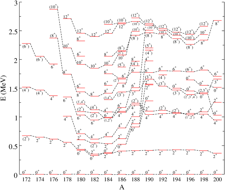
Figure 1: (Color online) Experimental energy level systematics for Hg isotopes. Only levels up to $E_{x}\sim$ 3.0 MeV are shown.

II The experimental data in the even-even Hg nuclei

The even-even Hg nuclei span a very large region of isotopes, starting with the lightest presently know ¹⁷²Hg nucleus (N=92), passing through the mid-shell point at N=104 at ¹⁸⁴Hg, all the way up to the N=126 neutron closed shell at ²⁰⁶Hg. Many experimental complementary methods have been used to disentangle the properties over such a large interval. These nuclei are extensively covered in the Nuclear Data Sheet reviews for A=172 Kibedi10 , A=174 Browne99 , A=176 Basu06 , A=178 Achter09 , A=180 Wu03 , A=182 Sing11 , A=184 Bagl10 , A=186 Bagl03 , A=188 Sing02 , A=190 Sing03 , A=192 Bagl12 , A=194 Sing06 , A=196 Xia07 , A=198 Xia02 , and A=200 Kondev07 , and span the region we concentrate on in the present paper. Moreover, we have incorporated the most recent papers (up to and including early 2013) in order to highlight the salient experimental features of the Hg nuclei,over the mass span from A=172 to mass A=200.

The yrast band structure for mass A=172 to A=176 have been studied using the highly-selective recoil decay tagging (RDT) technique sand09 ; jul01 ; muikku98 . Carpenter et al. carpent97 studied both the A=176 and A=178 Hg nuclei. Using Gammasphere at the Fragment Mass Analyzer (FMA), the yrast band structure could be considerably extended kondev99 ; kondev00 for both mass A=178 and A=180. Experiments, in the late 80’s simon86 ; drac88 showed hints of shape coexisting states. Recent developments in the experimental methods to study the nuclear structure properties of these neutron-deficient Hg nuclei, allowed to substantially increase the nuclear structure data basis: ($\beta^{+}$/EC)-decay of ¹⁸⁰Tl else11 and in-beam conversion-electron spectroscopy page11 . Besides the new information on the low-spin states below E${}_{x}\sim$ 2 MeV, lifetimes up to spin J^π = 8⁺(10⁺) have been measured from using Recoil-Decay tagged (RDT) $\gamma$-rays, using the recoil distance Doppler-shift (RDDS) method grahn09 ; scheck10 for mass A=180 and A=182. This recent information largely extends the early data (see refs. bindra95 ; wauters96 ; ma84 ). Except for mass A=184 (new results on E0 transitions from conversion electron and $\gamma$-ray studies scheck11 ), no new results have been obtained since the most recent NDS evaluations, as cited before.

For the mass A=196 and A=198 Hg isotopes, recent experiments using the HORUS cube $\gamma$-ray spectrometer and $\gamma-\gamma$ angular correlation measurements, made it possible to determine multipole mixing ratios, spins and energy spectra bern10 ; bern09 . Moreover, in the case of A=198, (p,t) two-neutron transfer reactions allowed to map out the presence of a number of 0⁺ states bern13 .

The experimental energy systematics derived from the above data set for the Hg nuclei is shown in Fig. 1 and spans the interval A=172 up to and including A=200. The systematics is limited (for the high-spin states) up to E${}_{x}\sim$ 3 MeV. For mass numbers A $\geq$ 190, above the energy of E${}_{x}\sim$ 1.5 MeV, a number of low-spin states without a unique spin-parity assignment from the NDS evaluations are not drawn (often states with negative parity and/or more spin possibilities).

In between mass A=178 progressing to the lower A=176-172 isotopes, no connecting dashed lines are drawn because the present data set does not contain unambiguous information in order to extend them (see, e.g., the behavior of the J^π=4⁺ state going from A=178 to A=176). What is clear though is that from mass A=180 and downwards, the 2${}^{+}_{1}$ excitation energy is steadily increasing (as well as the energy of the associated (4⁺) and (6⁺) states). The interval 180 $\leq$ A $\leq$ 188(190) exhibits the presence of a 0⁺, 2⁺, 4⁺, 6⁺, 8⁺, 10⁺ collective band structure with a “parabolic”-like energy dependence on N (with respect to the minimal energy of the 0${}^{+}_{2}$ state at N=102). For the heavier nuclei (A $>$ 190), the Hg structure exhibits an almost flat behavior of the excitation energy as a function of increasing mass number A (or neutron number N). The observed 0${}^{+}_{1}$, 2${}^{+}_{1}$, 4${}^{+}_{1}$, 2${}^{+}_{2}$,… sequence seems to be pointing out the appearance of a $\gamma$-soft structure.

In the present paper, we cover the whole interval 172 $\leq$ A $\leq$ 200, but in the discussion mainly concentrate on the A=180-188(190) region which forms a challenge to theoretical model approaches. The energy systematics as shown in Fig. 1 indicates three distinct structures: a less deformed one for mass A $>$ 190, a region where a more collective structure intrudes to low excitation energies in the region 180 $\leq$ A $\leq$ 188, and a region where the lowest 2⁺ state (and associated higher-spin states for the yrast part) exhibits a steadily increasing excitation energy (A $\leq$ 178).

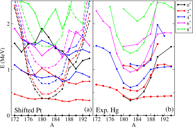
Figure 2: (Color online) Comparison between the “shifted” theoretical energy spectra for Pt (panel (a)) (see text and Figure 12 in  García-Ramos and Heyde (2009)) and the experimental Hg low-lying energy spectra (panel (b)).

III The Interacting Boson Model with configuration mixing formalism

III.1 The formalism

The IBM-CM allows the simultaneous treatment and mixing of several boson configurations which correspond to different particle–hole (p–h) shell-model excitations duval82 . On the basis of intruder spin symmetry hey92 ; hey94 ; coster96 ; oros99 , no distinction is made between particle and hole bosons. Hence, the model space which includes the regular proton 2h configurations and a number of valence neutrons outside of the N=82 closed shell (corresponding to the standard IBM treatment for the Hg even-even nuclei) as well as the proton 4h-2p configurations and the same number of valence neutrons corresponds to a $[N]\oplus[N+2]$ boson space ($N$ being the number of active protons, counting both proton holes and particles, plus the number of valence neutrons outside the N=82 closed shell, divided by $2$ as the boson number). Consequently, the Hamiltonian for two configuration mixing can be written as

$$\hat{H}=\hat{P}^{{\dagger}}_{N}\hat{H}^{N}_{\rm ecqf}\hat{P}_{N}+\hat{P}^{{\dagger}}_{N+2}\left(\hat{H}^{N+2}_{\rm ecqf}+\Delta^{N+2}\right)\hat{P}_{N+2}\ +\hat{V}_{\rm mix}^{N,N+2}~{},$$ (1)

where $\hat{P}_{N}$ and $\hat{P}_{N+2}$ are projection operators onto the $[N]$ and the $[N+2]$ boson spaces, respectively, $\hat{V}_{\rm mix}^{N,N+2}$ describes the mixing between the $[N]$ and the $[N+2]$ boson subspaces, and

$$\hat{H}^{i}_{\rm ecqf}=\varepsilon_{i}\hat{n}_{d}+\kappa^{\prime}_{i}\hat{L}\cdot\hat{L}+\kappa_{i}\hat{Q}(\chi_{i})\cdot\hat{Q}(\chi_{i}),$$ (2)

is the extended consistent-Q Hamiltonian (ECQF) warner83 with $i=N,N+2$, $\hat{n}_{d}$ the $d$ boson number operator,

$$\hat{L}_{\mu}=[d^{\dagger}\times\tilde{d}]^{(1)}_{\mu},$$ (3)

the angular momentum operator, and

$$\hat{Q}_{\mu}(\chi_{i})=[s^{\dagger}\times\tilde{d}+d^{\dagger}\times s]^{(2)}_{\mu}+\chi_{i}[d^{\dagger}\times\tilde{d}]^{(2)}_{\mu}~{},$$ (4)

the quadrupole operator. We are not considering the most general IBM Hamiltonian in each Hilbert space, [N] and [N+2], but we are restricting to a ECQF formalism warner83 ; lipas85 in each subspace. This approach has been shown to be a rather good approximation in many calculations and in particular in two recent papers describing the Pt isotopes García-Ramos and Heyde (2009); Garc11 .

The parameter $\Delta^{N+2}$ can be associated with the energy needed to excite two proton particles across the Z=82 shell gap, giving rise to 2p-2h excitations, corrected for the pairing interaction gain and including monopole effects hey85 ; hey87 . The operator $\hat{V}_{\rm mix}^{N,N+2}$ describes the mixing between the $N$ and the $N+2$ configurations and is defined as

$$\hat{V}_{\rm mix}^{N,N+2}=w_{0}^{N,N+2}(s^{\dagger}\times s^{\dagger}+s\times s)+w_{2}^{N,N+2}(d^{\dagger}\times d^{\dagger}+\tilde{d}\times\tilde{d})^{(0)}.$$ (5)

The $E2$ transition operator for two-configuration mixing is subsequently defined as

$$\hat{T}(E2)_{\mu}=\sum_{i=N,N+2}e_{i}\hat{P}_{i}^{\dagger}\hat{Q}_{\mu}(\chi_{i})\hat{P}_{i}~{},$$ (6)

where the $e_{i}$ ($i=N,N+2$) are the effective boson charges and $\hat{Q}_{\mu}(\chi_{i})$ the quadrupole operator defined in equation (4).

In section III.2 we present the methods used in order to determine the parameters appearing in the IBM-CM Hamiltonian as well as in the $\hat{T}(E2)$ operator.

The wave function, within the IBM-CM, can be described as

$$\Psi(k,JM) = \sum_{i}a^{k}_{i}(J;N)\psi((sd)^{N}_{i};JM)$$ (7)

$$+ \ \sum_{j}b^{k}_{j}(J;N+2)\psi((sd)^{N+2}_{j};JM)~{},$$

where $k$, $i$, and $j$ are rank numbers. The weight of the wave function contained within the $[N]$-boson subspace, can then be defined as the sum of the squared amplitudes $w^{k}(J,N)\equiv\sum_{i}\mid a^{k}_{i}(J;N)\mid^{2}$. Likewise, one obtains the content in the $[N+2]$-boson subspace.

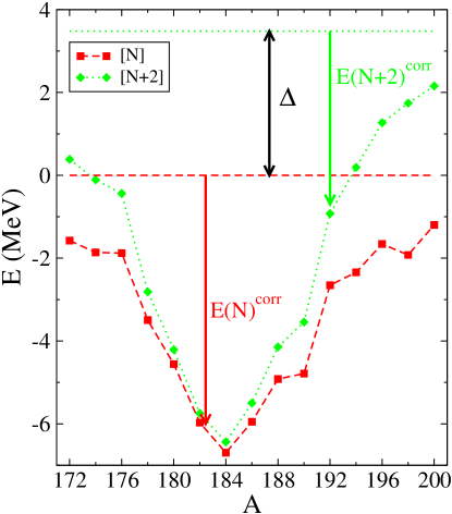
Figure 3: (Color online) Absolute energy of the lowest regular and lowest intruder states for ^172-200Hg. The arrows correspond to the correlation energies in the N and N+2 subspaces.

III.2 The fitting procedure: energy spectra and absolute B(E2) reduced transition probabilities

Here, we present the way in which the parameters of the Hamiltonian (1), (2), and (5) and the effective charges in the $\hat{T}(E2)$ transition operator (6) have been determined. We study the range ¹⁷²Hg to ²⁰⁰Hg thereby covering a major part of the neutron N=82-126 shell.

Table 1: Energy levels, characterized by $J^{\pi}_{i}$, included in the energy fit, if known, and the assigned $\sigma$ values in keV.

Error (keV)	States
$\sigma=0.1$	$2_{1}^{+}$
$\sigma=1$	$4_{1}^{+},0_{2}^{+},2_{2}^{+}$
$\sigma=10$	$2_{3}^{+},3_{1}^{+},4_{2}^{+},6_{1}^{+},8_{1}^{+}$
$\sigma=100$	$2_{4}^{+},3_{1}^{+},4_{3}^{+},6_{2}^{+}$

In the fitting procedure carried out here, we try to obtain the best possible agreement with the experimental data including both the excitation energies and the B(E2) reduced transition probabilities. Using the expression of the IBM-CM Hamiltonian, as given in equation (1), and of the E2 operator, as given in equation (6), in the most general case $13$ parameters show up. We impose a constraint of obtaining parameters that change smoothly in passing from isotope to isotope. Note also that we constrained $\varepsilon_{N+2}=0$, $\kappa^{\prime}_{N}=0$, and $\kappa^{\prime}_{N+2}=0$. We have explored in detail the validity of this assumption and we have found very little improvement in the value of $\chi^{2}$ when releasing those parameters. On the other hand, we have kept the value that describes the energy needed to create an extra particle-hole pair ($2$ extra bosons) constant, i.e., $\Delta^{N+2}=3480$ keV, and have also put the constraint of keeping the mixing strengths constant too, i.e., $w_{0}^{N,N+2}=w_{2}^{N,N+2}=20$ keV for all the Hg isotopes. We also have to determine for each isotope the effective charges of the $E2$ operator. This finally leads to $7$ parameters to be varied in each nucleus.

To fix the value of $\Delta^{N+2}=3480$ keV we have taken into account the strong similarity that shows up in Fig. 2 between, on one side (see panel (a)), the Pt spectra resulting from Refs. García-Ramos and Heyde (2009); Garc11 , but switching off the mixing term and shifting the value of $\Delta$ to $3480$ keV and, on the other side (see panel (b)), the experimental energy systematics of Hg isotopes. This value of $\Delta^{N+2}$ gives rise to degenerate $2_{1}^{+}$ and $0_{2}^{+}$ states at A=182, which is consistent with the experimental situation observed in the Hg nuclei. To fix the value of the mixing strengths we considered that the corresponding value for the Pt nuclei was fixed to $50$ keV García-Ramos and Heyde (2009), while for the Pb, to a smaller strength of $18$ keV fossion03 ; helle05 . We performed a set of exploratory calculations between the two latter values and found that the best agreement corresponds to $w_{0}^{N,N+2}=w_{2}^{N,N+2}=20$ keV, although values in the range of $20-30$ keV provided a very similar agreement.

Table 2: Hamiltonian and $\hat{T}(E2)$ parameters resulting from the present study. All quantities have the dimension of energy (given in units of keV), except $\chi_{N+2}$ which is dimensionless and $e_{N}$ and $e_{N+2}$ which are given in units $\sqrt{\mbox{W.u.}}$ The remaining parameters of the Hamiltonian, i.e., $\chi_{N}$, $\varepsilon_{N+2}$, $\kappa^{\prime}_{N}$, and $\kappa^{\prime}_{N+2}$ are equal to zero, except $\Delta^{N+2}=3480$ keV and $w_{0}^{N,N+2}=w_{2}^{N,N+2}=20$ keV.

Nucleus	$\varepsilon_{N}$	$\kappa_{N}$	$\chi_{N}$	$\kappa_{N+2}$	$\chi_{N+2}$	$e_{N}$	$e_{N+2}$
172Hg	845.0	-41.38	0.01	-20.70	-1.29	-	-
174Hg	888.6	-40.21	0.02	-19.63	1.25	-	-
176Hg	906.4	-34.99	0.02	-27.99	0.01	-	-
178Hg	1032.4	-50.27	0.15	-37.56	0.13	-	-
180Hg	1152.1	-54.39	0.36	-38.72	-0.19	1.38	2.41
182Hg	1253.4	-58.46	0.39	-39.91	-0.17	1.11	2.24
184Hg	1321.9	-58.12	0.41	-38.74	-0.11	1.14	1.94
186Hg	1097.6	-56.95	0.36	-39.57	-0.16	1.07	2.11
188Hg	839.4	-53.17	0.20	-38.61	-0.17	1.42	2.13
190Hg	703.3	-57.59	0.13	-42.57	0.01	1.42∗	2.13∗
192Hg	697.3	-42.57	0.25	-26.55	-0.60	1.42∗	2.13∗
194Hg	615.8	-44.49	0.19	-21.34	-1.32	1.42∗	2.13∗
196Hg	545.9	-39.79	0.16	-18.00	-0.85	1.81	2.72∗
198Hg	449.2	-54.08	0.31	-18.00	-0.85	1.83	-
200Hg	499.3	-45.73	1.07	-18.00	-0.85	1.97	-

The $\chi^{2}$ test is used in the fitting procedure in order to extract the optimal solution. The $\chi^{2}$ function is defined in the standard way as

$$\chi^{2}=\frac{1}{N_{data}-N_{par}}\sum_{i=1}^{N_{data}}\frac{(X_{i}(data)-X_{i}(IBM))^{2}}{\sigma_{i}^{2}},$$ (8)

where $N_{data}$ is the number of experimental data, $N_{par}$ is the number of parameters used in the IBM fit, $X_{i}(data)$ describes the experimental excitation energy of a given excited state (or an experimental B(E2) value), $X_{i}(IBM)$ denotes the corresponding calculated IBM-CM value, and $\sigma_{i}$ is an error assigned to each $X_{i}(data)$ point.

The $\chi^{2}$ function is defined as a sum over all data points including excitation energies as well as absolute B(E2) values. The minimization is carried out using $\varepsilon_{N}$, $\kappa_{N}$, $\kappa_{N+2}$, $\chi_{N}$, $\chi_{N+2}$, $e_{N}$ and $e_{N+2}$ as free parameters, having fixed $\varepsilon_{N+2}=0$, $\kappa^{\prime}_{N}=0$, $\kappa^{\prime}_{N+2}=0$, $\Delta^{N+2}=3480$ keV and $w_{0}^{N,N+2}=w_{2}^{N,N+2}=20$ keV as described before. We minimize the $\chi^{2}$ function for each isotope separately using the package MINUIT minuit which allows to minimize any multi-variable function. In some of the lighter Hg isotopes, due to the small number of experimental data, the values of some of the free parameters could not be fixed unambiguously using the above fitting procedure. Moreover, for the heavier isotopes ($A>194$), that part of the Hamiltonian corresponding to the intruder states is fixed such as to guarantee that those states appear well above the regular ones, that is, above $3$ MeV. In some cases due to the lack of experimental data the effective charges could not be determined. For $A>196$, $e_{N+2}$ cannot be determined because the B(E2) values are insensitive to this parameter. However, for completeness we have taken the effective charges of ^190-194Hg equal to the ones of ¹⁸⁸Hg while $e_{N+2}$ in ¹⁹⁶Hg was obtained by imposing the constraint to have the same ratio $e_{N+2}/e_{N}$ as for ¹⁸⁸Hg.

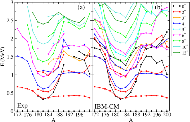
Figure 4: (Color online) Experimental excitation energies (up to $E_{x}\approx 3.0$ MeV) (panel (a)) and the theoretical results (panel (b)), obtained from the IBM-CM.

As input values, we have used the excitation energies of the levels presented in table 1. In this table we also give the corresponding $\sigma$ values. We stress that the $\sigma$ values do not correspond to experimental error bars, but they are related with the expected accuracy of the IBM-CM calculation to reproduce a particular experimental data point. Thus, they act as a guide so that a given calculated level converges towards the corresponding experimental level. The $\sigma$ ($0.1$ keV) value for the $2_{1}^{+}$ state guarantees the exact reproduction of this experimental most important excitation energy, i.e., the whole energy spectrum is normalized to this experimental energy. The states $4_{1}^{+},0_{2}^{+}$ and $2_{2}^{+}$ are considered as the most important ones to be reproduced ($\sigma=1$ keV). The group of states $2_{3}^{+}$, $3_{1}^{+}$, $4_{2}^{+}$, $6_{1}^{+}$, and $8_{1}^{+}$ ($\sigma=10$ keV) and $2_{4}^{+}$, $3_{1}^{+}$, $4_{3}^{+}$, and $6_{2}^{+}$ ($\sigma=100$ keV) should also be well reproduced by the calculation to guarantee a correct moment of inertia for the yrast band and the structure of the pseudo-$\gamma$ and $0_{2}^{+}$ bands. Besides, in specific nuclei, A $=186,190,$ and 196, additional states have been taken into account, but in all cases those states have an excitation energy below $2-2.5$ MeV and $J<10$. Note also that if two, or more, angular momenta are assigned to a given level (see the references  Kibedi10 ; Browne99 ; Basu06 ; Achter09 ; Wu03 ; Sing11 ; Bagl10 ; Bagl03 ; Sing02 ; Sing03 ; Bagl12 ; Sing06 ; Xia07 ; Xia02 ; Kondev07 and/or the extra references given in Section  II), those levels are not included in the fitting procedure.

In the case of the $E2$ transitions rates, we have used the available experimental data involving the states presented in table 1, restricted to those $E2$ transitions for which absolute B(E2) values are known. Additionally we have taken a value of $\sigma$ that corresponds to $10\%$ of the B(E2) values or to the experimental error bar if larger, except for the transition $2_{1}^{+}\rightarrow 0_{1}^{+}$ where a smaller value of $\sigma$ ($0.1$ W.u.) was taken, therefore normalizing to the experimental $B(E2;2^{+}_{1}\rightarrow 0^{+}_{1})$ value. The experimental data we have used result from the data appearing in references  Kibedi10 ; Browne99 ; Basu06 ; Achter09 ; Wu03 ; Sing11 ; Bagl10 ; Bagl03 ; Sing02 ; Sing03 ; Bagl12 ; Sing06 ; Xia07 ; Xia02 ; Kondev07 , complemented with the specific references already presented in Section II. In the present fit, we have not included relative B(E2) values, which may well slightly modify the effective charges obtained at present.

This has resulted in the values of the parameters for the IBM-CM Hamiltonian, as given in table 2. In the case of ^172-178Hg and ^190-196Hg, the value of the effective charges, or part of them, cannot be determined because not a single absolute B(E2) value is known or $\chi^{2}$ is insensitive to their values. However, for completeness we have taken the value of the effective charges in ^190-194Hg. to be the same as in ¹⁸⁸Hg (or as having the same ratio for ¹⁹⁶Hg).

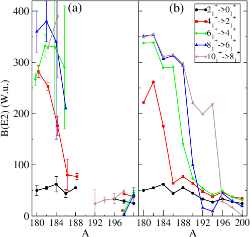
Figure 5: (Color online) Comparison of the absolute B(E2) reduced transition probabilities along the yrast band, given in W.u. The panel (a) corresponds to known experimental data and the panel (b) to the theoretical IBM-CM results.

III.3 Correlation energy in the configuration mixing approach

Intruder configurations should appear, by construction, at an excitation energy that is much higher than the regular configurations. This is so because of the large energy needed to create the 2p-2h excitation across the Z=82 closed shell. In the case of the Hg nuclei, $\Delta^{N+2}=3480$ keV, but according to reference hey87 the single-particle energy cost has to be corrected because of the strong pairing energy gain when forming two extra $0^{+}$ coupled (particle and hole) pairs, the quadrupole energy gain when opening up the proton shell, as well as by the monopole correction caused by a change in the single-particle energy gap at Z=82 as a function of the neutron number. In some cases, specifically around the mid-shell point at N=104, the energy gain through these correlations can become so large that the intruder configurations intrude to be located below the energy of the regular configurations. In this case one speaks about “islands of inversion” heyde11 .

A different way to understand the relative position of regular and intruder configurations is to consider the energy of the lowest lying regular and intruder state. The regular configuration, which corresponds to a spherical or slightly deformed shape, can be considered as the “reference” state and to have zero energy. This configuration will be lowered, as a function of neutron number, because of the correlation energy due to the quadrupole interaction (in our case using the IBM). On the other hand, the intruder configuration corresponds to a more strongly deformed shape. Its energy will then be equal to $\Delta^{N+2}$ corrected by the correlation energy, this time within the (N+2) configuration. This situation is illustrated in Fig. 3 where it is clearly appreciated how the energies of both configurations can come very close in energy, depending on the balance between the off-set $\Delta^{N+2}$ and the difference in the correlation energy $E(N+2)^{corr}-E(N)^{corr}$.

One observes that around mid shell, both configurations are fairly close in energy although the energy of the regular configuration is below the intruder configuration in all cases. However, near the beginning and the end of the shell, this energy difference becomes much larger. Note that the value of $\Delta^{N+2}$ constrains the parabolic shape of the intruder energy systematics at both sides of the shell. Near the doubly-closed shells, the $0^{+}$ ground state is approximately spherical and the corresponding correlation energy will be small. Therefore, the largest possible excitation energy for the lowest intruder configuration should appear at an energy below $\Delta^{N+2}$, simply because the correlation energy for the intruder configuration (having two more nucleon pairs) is larger than the correlation energy for the regular states. Consequently, the parabolic behavior which shows up around mid shell will be eroded for the lightest and the heaviest isotopes, resulting in a rather flat energy systematics and therefore intruder configurations result at an energy lower than expected.

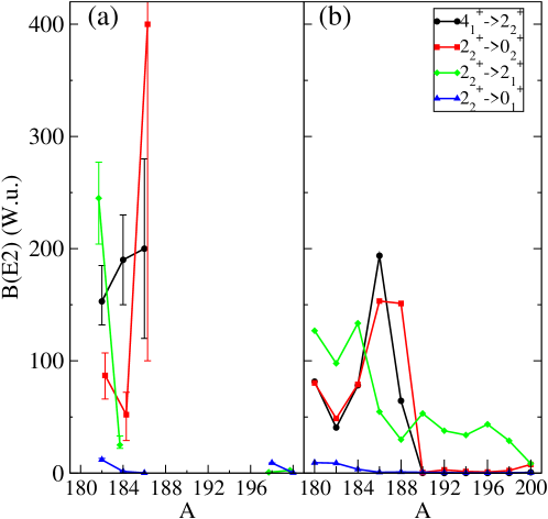
Figure 6: (Color online) Comparison of the few non-yrast absolute B(E2) reduced transition probabilities, given in W.u. The panel (a) corresponds to the few known experimental data, the panel (b) to the theoretical IBM-CM results.

III.4 Detailed comparison between the experimental data and the IBM-CM results: energy spectra and electric quadrupole properties

In the present subsection, we compare the experimental energy spectra with the energy spectra as obtained from the IBM-CM, for the limited data set (with excitation energy $E_{x}$ less than $\approx$ 3.0 MeV), so as to be able to carry out a detailed comparison of the experimental data (panel (a) of Fig. 4) and the calculations (panel (b) of Fig. 4). In comparing both panels of Fig. 4 one can observe a rather good overall agreement. Note that the energy of the $2_{1}^{+}$ level matches perfectly the experimental one because we used precisely this level to constrain the calculation. For the other levels we reproduce correctly the observed almost parabolic behavior of the energy levels with a lowest excitation energy of the second $0^{+}_{2}$ state at N=102 (A=182) (near neutron mid-shell), while a rather flat behavior of the excitation energies as a function of increasing neutron number for the heavier Hg nuclei (A $\geq$ 190) shows up, consistent with the data. For the nuclei with mass number below A=180 (172 $\leq$ A $\leq$ 180), we perfectly match the steady increase of the energy levels with decreasing mass number A. We point out that for the nuclei near mid-shell, the experimental energy systematics is reproduced up to angular momentum $J=12$, although states with $J=10$ and $J=12$ have not been included in the fitting procedure. In general, the agreement with the data is better for the states with even $J$ values, while the calculated theoretical energy levels with odd $J$ values appear systematically above the experimental excitation energies.

We carry out a more detailed comparison for both the energies and E2 properties in the region where shape coexistence shows up most clearly (180 $\leq$ A $\leq$ 188) in the later part of this section.

A more stringent test than a good reproduction of the energy systematics comes from calculating those observables that probe the corresponding wave functions and a comparison with the data. Recent experimental efforts have given rise to absolute B(E2) values along the yrast band, deduced from lifetime measurements grahn09 ; scheck10 , as well as through Coulomb excitation at ISOLDE-CERN Isol12 ; lipska13 , the latter also giving first results for the quadrupole moments of the $2^{+}_{1}$ and $2^{+}_{2}$ states.

The systematics for a number of important E2 transitions and the electric quadrupole moments are presented in figures 5, 6, and 7, respectively.

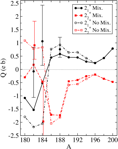
Figure 7: (Color online) IBM-CM values of the quadrupole moments of the states $2_{1}^{+}$ and $2_{2}^{+}$ for ^180-200Hg. Quadrupole moments given in units $e\,b$. The dash-dotted lines indicate the quadrupole moments when the mixing Hamiltonian is switched off, corresponding to the unperturbed states.

Because these figures highlight only the specific set of important B(E2) values, we detail the comparison between the present theoretical study and the existing data (which is most documented in the 180 $\leq$ A $\leq$ 190 region of shape coexistence) in tables 3, 4, and 5 in which we compare the experimental absolute B(E2) values as well as the relative B(E2) values, respectively, with the corresponding IBM-CM theoretical results.

In Fig. 5 (panel (a)) one observes a rather constant value for the $B(E2;2^{+}_{1}\rightarrow 0^{+}_{1})$ at approximately $\approx$ 50 W.u., and very large B(E2) values for the higher spin values, with a particular interesting behavior for the $B(E2;4^{+}_{1}\rightarrow 2^{+}_{1})$ which is dropping from A=182 towards a more stable value (see also the calculated variation in Fig. 5 (panel (b))) starting at A=186 and onwards. This very clearly shows an important change in the structure of the $2^{+}_{1}$ and $2^{+}_{2}$ states passing through the region A=180 to A=188. We come back later to this most important observation, that highlights a particular mixing pattern between those $2^{+}$ states. Concerning the high-spin $10^{+}_{1}$ to $8^{+}_{1}$ E2 transition in the region A=190 to A=194, a pronounced collective character still exits. This is indeed what is expected in the IBM. In the case of ^196-198Hg the agreement is improved due to the reduction in the number of available bosons.

In Fig. 6 (panel (a)), we show the few non-yrast absolute B(E2) values known (see also table 5). Here, one observes larger $B(E2;4^{+}_{1}\rightarrow 2^{+}_{2})$ values as compared to the corresponding yrast B(E2) value (starting at A=186) which is again a clear hint of the changing mixing between the unperturbed configurations making up the lowest two $2^{+}$ states. The comparison with the theoretical values (see Fig. 6 panel (b)), where a maximal $B(E2;4^{+}_{1}\rightarrow 2^{+}_{2})$ value is obtained for A=184 looks interesting, the more because the $B(E2;2^{+}_{2}\rightarrow 0^{+}_{2})$ exhibits a similar behavior, pointing out a very specific change in the composition of the $2^{+}$ states (see also Section  III.5 for a more extensive discussion).

The above observations are most interesting because one observes a smooth behavior in the excitation energy of the $2^{+}_{1,2}$ states when moving from A=180 towards A=188, still there must be a major change in the wave functions of these states. The particular mixing between the $2^{+}_{1,2}$ regular and intruder configuration is dramatically present in the calculated spectroscopic quadrupole moments as shown in Fig. 7. Up to mass A=184, the nucleus in which our calculations result in a close to equal mixing between the regular and intruder configurations (see Fig. 12), the intruder configuration dominates in the $2^{+}_{1}$ state, giving rise to the negative sign, and opposite to the $2^{+}_{2}$ state. For masses above A=184, the calculations result in a $2^{+}_{1}$ state with increasing weight for the regular configuration, and the opposite for the $2^{+}_{2}$ state, up to A=188. From mass A=190 onwards, both $2^{+}_{1,2}$ are described by wave functions within the regular configuration space only. We complement this figure by also including the quadrupole moments for the unperturbed lowest intruder and regular state (obtained from switching off the mixing Hamiltonian).

We present in figures 8 and 9 the experimental and theoretical energy spectra, respectively (up to $E_{x}=2-3$ MeV), concentrating on the region where the “coexistence” of two structures, with their specific energy scale, becomes obvious: one less and one more deformed configuration. In Fig. 8, we combine the energies and the experimental B(E2) values. We give the absolute B(E2) values when known and the relative ones, mainly at the low spin part of the energy spectra.

A first point is the fact that the proximity of the $2^{+}_{1}$ and $2^{+}_{2}$ states within an energy of $\approx$ 180 keV from A=180 up to A=184 indicates rather strong mixing between the two configurations. An indicator for the mixing shows up from the relative B(E2) values de-exciting the $2^{+}_{2}$ state. Using a normalization to 100 for the $B(E2;2^{+}_{2}\rightarrow 0^{+}_{2})$, the value of $B(E2;2^{+}_{2}\rightarrow 0^{+}_{1})$ decreases from $38(3)$ W.u. (A=180), $13(5)$ W.u. (A=182), $2.9(1.2)$ W.u. (A=184) down to $0.01$ W.u. (A=186), moving quickly down for heavier masses. The observation of a strong E0 component in the decay of the $2^{+}_{2}$ state into the $2^{+}_{1}$ state  page11 ; scheck11 is a quantitative indicator of important mixing in the wave functions  joshi94 ; wood99 . This important information, extended with the large absolute B(E2) values originating from the yrast $10^{+}$,…,$6^{+}$ states, allows us to separate the levels into two families. This separation is substantiated by the much smaller and fairly constant $B(E2;2^{+}_{1}\rightarrow 0^{+}_{1})$ value $\approx$ 50 W.u.

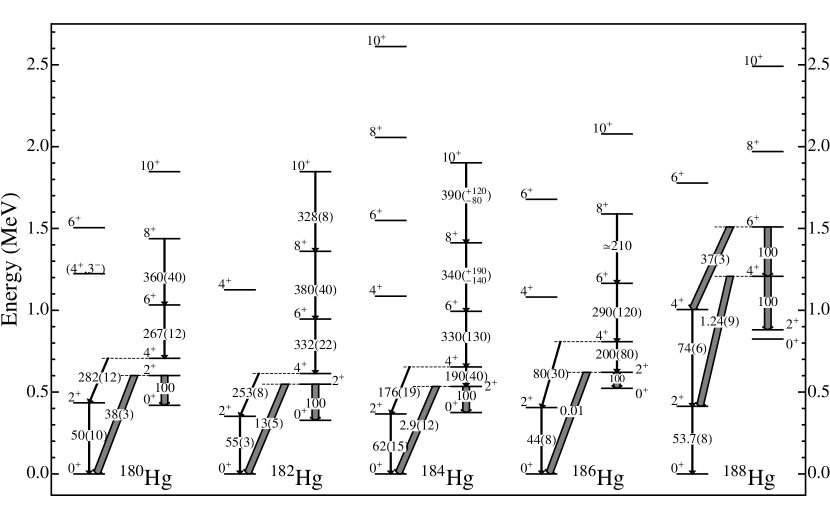
Figure 8: Experimental excitation energies, absolute B(E2) transition rates and relative B(E2) values for selected states in ^180-188Hg. Thin lines correspond to absolute B(E2) values while the thicker ones to relative B(E2) values.

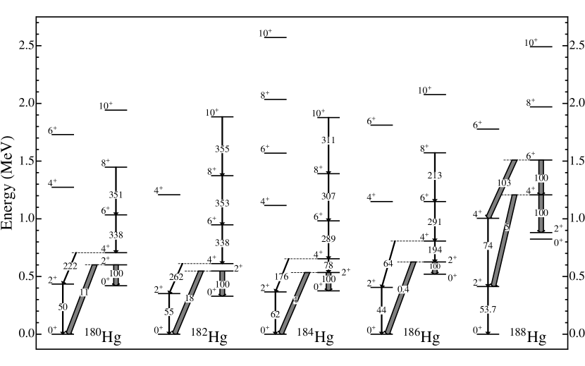
Figure 9: Theoretical excitation energies, absolute B(E2) transition rates and relative B(E2) values for selected states in ^180-188Hg. Thin lines correspond to absolute B(E2) values while the thicker ones to relative B(E2) values.

We also notice that the E2 decay from the $4^{+}_{1}$ into the $2^{+}_{1,2}$ levels is such that from mass A=184 onwards, the $B(E2;4^{+}_{1}\rightarrow 2^{+}_{2})$ value (which is still almost equal to the $B(E2;4^{+}_{1}\rightarrow 2^{+}_{1})$ value) starts to dominate quickly when moving towards mass A=188, with relative B(E2) values changing from 200(80) over 80(30) for A=186, up to $100$ over $1.24(9)$ for A=188. This indicates that the intruder structure is quickly moving up in energy relative to the regular structure. Combining all the available data: excitation energies, absolute and relative B(E2) values, it shows that only in A=186 the coupling between, on one side the $0^{+}_{1},2^{+}_{1},4^{+}_{2}$ states, and, on the other side the $0^{+}_{2},2^{+}_{2},4^{+}_{1}$ states, as expressed by the weights $w^{k}(J,N)$ (see expression (7)), comes out to be less than $20\%$ (see Fig. 12) consistent with rather weakly coupled bands.

In A=188, perturbations are arising for the $4^{+}$ and $6^{+}$ levels, as indicated by the relative B(E2) values originating from the decay of the $6^{+}_{1}$ state, having a clear preference for the $4^{+}_{2}$ level. Here it looks like the $4^{+}_{1}$ state has become a member of the less collective band.

In view of the above analyses of the experimental available data, the present separation into two families can be made. However, the relative changes in energy differences at the lower end of the intruder band as well as the relative B(E2) values, connecting the two bands, unambiguously show important mixing between the $2^{+}$ members of the two families.

In Fig. 9, we compare with the corresponding theoretical energy spectra and B(E2) values, denoting the absolute values and relative B(E2) values, in order to allow an easy comparison with the data shown in Fig. 8. The overall structure, both on energy spectra as well as on the absolute B(E2) values, agrees rather well with the corresponding experimental figure. Because at the lower end of the intruder band, the deexcitation largely favors decay into the $2^{+}_{1}$ state rather than into the $2^{+}_{2}$ state and thus makes it very difficult to obtain absolute B(E2) values, we show the relative B(E2) values, normalized at 100 for the $B(E2;2^{+}_{2}\rightarrow 0^{+}_{2})$ value. One observes a steady increase of the ratio from A=188 down to A=180, consistent with the experimental data, with a clear dominance of the inband E2 decay. This is consistent with the fact that the wavefunction of the ground state $0^{+}_{1}$ state is mainly of regular character, the $0^{+}_{2}$ mainly of intruder character, whereas the nature of the $2^{+}_{2}$ exhibits a global increase of its regular character going from A=188 down to A=182 (see Fig. 12).

Moving into the heavier Hg isotopes (beyond A=190), showing the experimental and theoretical spectra of ¹⁹²Hg (Fig. 10) as an example, the occurrence of shape coexistence seems to be dissolved.

Figure 10: Detailed comparison between the experimental energy spectrum and the calculated IBM-CM spectrum for ¹⁹²Hg.

Inspecting the systematics of the Hg nuclei, from A=188 and onwards up to A$\approx 200$, the appearance of a set of close-lying high-spin states, i.e., the $12^{+},10^{+}$ and $8^{+}$ state is striking (see Fig. 1). From measurements of the magnetic moment of the $12^{+}_{1},10^{+}_{1}$ states in the nuclei A=188 to A=196  Stone05 , the deduced g-factor varies between $-0.19(11)\mu_{N}$ and $-0.24(4)\mu_{N}$, which corresponds very well with the g-factor characterizing the neutron $\nu 1i_{13/2}$ single-particle orbital, pointing towards a clear-cut one broken-pair character of $(1i_{13/2})^{2};J^{\pi}$ structure. The slight rise in excitation energy approaching the neutron N=126 shell closure is consistent with the picture of a state becoming less collective and more shell-model like in its character.

Figure 11: Experimental values of $B(E2;12^{+}_{1}\rightarrow 10^{+}_{1})$. Data are taken from the corresponding NDS references Sing03 ; Bagl12 ; Sing06 ; Xia07 ; Xia02 .

A naïve shell-model point-of-view indeed shows the filling of the $\nu 1i_{13/2}$ orbital in between ¹⁸⁰Hg and ¹⁹⁴Hg. Because of pairing correlations, one can expect an effect on the E2 transition probability connecting the $12^{+}_{1}$ state with the $10^{+}_{1}$ state. Experimental data are available on this transition, giving rise to B(E2) values and partly for the $10^{+}_{1}$ state decaying to the $8^{+}_{1}$ state (see A=190 Sing03 , A=192 Bagl12 , A=194 Sing06 , A=196 Xia07 , A=198 Xia02 ). For the $B(E2;12^{+}_{1}\rightarrow 10^{+}_{1})$ reduced transition probability, one notices a decreasing value from the largest known value of 43(12) W.u. (in A=198) coming down to 9(1) W.u. (in A=190). This variation, as shown in Fig. 11, looks quite linear with A and might reflect the effect of the occupation of the $1i_{13/2}$ neutron orbital, which, for a pure seniority non-changing $v=2\rightarrow v=2$ E2 transition would change with the factor $[u^{2}(1i_{13/2})-v^{2}(1i_{13/2})]$.

Table 3: Comparison of the experimental absolute B(E2) values (given in units of W.u.) with the IBM-CM Hamiltonian results. Data are taken from the Nuclear Data Sheets Kibedi10 ; Browne99 ; Basu06 ; Achter09 ; Wu03 ; Sing11 ; Bagl10 ; Bagl03 ; Sing02 ; Sing03 ; Bagl12 ; Sing06 ; Xia07 ; Xia02 ; Kondev07 , complemented with references presented in section II.

Isotope	Transition	Experiment	IBM-CM
180Hg	$2_{1}^{+}\rightarrow 0_{1}^{+}$	50(10)	50
	$4_{1}^{+}\rightarrow 2_{1}^{+}$	282(12)	223
	$6_{1}^{+}\rightarrow 4_{1}^{+}$	267(12)	338
	$8_{1}^{+}\rightarrow 6_{1}^{+}$	360(40)	351
182Hg	$2_{1}^{+}\rightarrow 0_{1}^{+}$	55(3)	55
	$4_{1}^{+}\rightarrow 2_{1}^{+}$	253(8)	262
	$6_{1}^{+}\rightarrow 4_{1}^{+}$	332(22)	338
	$8_{1}^{+}\rightarrow 6_{1}^{+}$	380(40)	354
	$10_{1}^{+}\rightarrow 8_{1}^{+}$	328(8)*	355
	$2_{2}^{+}\rightarrow 0_{1}^{+}$	11.8(12)*	9
	$2_{2}^{+}\rightarrow 0_{2}^{+}$	87$(^{+20}_{-23})$*	49
	$2_{2}^{+}\rightarrow 2_{1}^{+}$	245$(^{+32}_{-41})$*	98
	$4_{1}^{+}\rightarrow 2_{2}^{+}$	153$(^{+32}_{-21})$*	41
184Hg	$2_{1}^{+}\rightarrow 0_{1}^{+}$	62(15)	62
	$4_{1}^{+}\rightarrow 2_{1}^{+}$	176(19)	176
	$6_{1}^{+}\rightarrow 4_{1}^{+}$	330(130)	289
	$8_{1}^{+}\rightarrow 6_{1}^{+}$	340$(^{+190}_{-140})$	306
	$10_{1}^{+}\rightarrow 8_{1}^{+}$	390$(^{+120}_{-80})$*	311
	$2_{2}^{+}\rightarrow 0_{1}^{+}$	1.4(3)*	3.4
	$2_{2}^{+}\rightarrow 0_{2}^{+}$	52(20)*	79
	$2_{2}^{+}\rightarrow 2_{1}^{+}$	25(8)*	133
	$4_{1}^{+}\rightarrow 2_{2}^{+}$	190(40) and 500(80)*	78
186Hg	$2_{1}^{+}\rightarrow 0_{1}^{+}$	44(8)	44
	$4_{1}^{+}\rightarrow 2_{1}^{+}$	80(30)	64
	$6_{1}^{+}\rightarrow 4_{1}^{+}$	290(120)	291
	$8_{1}^{+}\rightarrow 6_{1}^{+}$	$\approx 210$	313
	$2_{2}^{+}\rightarrow 0_{1}^{+}$	$(0.0,+0.2)$*	0.6
	$2_{2}^{+}\rightarrow 0_{2}^{+}$	400(300) and $>140$*	153
	$4_{1}^{+}\rightarrow 2_{2}^{+}$	200(80) and 490$(^{+240}_{-100})$*	194

Table 4: See caption of Table 3.

Isotope	Transition	Experiment	IBM-CM
188Hg	$2_{1}^{+}\rightarrow 0_{1}^{+}$	53.7(8)	54
	$4_{1}^{+}\rightarrow 2_{1}^{+}$	74(6)	74
190Hg	$(12_{1}^{+})\rightarrow(10_{1}^{+})$	9(1)*	216**
192Hg	$(10_{1}^{+})\rightarrow 8_{1}^{+}$	24$(^{+27}_{-24})$*	199**
	$(12_{1}^{+})\rightarrow 10_{1}^{+}$	19(4)*	186**
194Hg	$(10_{1}^{+})\rightarrow 8_{1}^{+}$	31(6)*	218**
	$(12_{1}^{+})\rightarrow(10_{1}^{+})$	24(2)*	193**
196Hg	$2_{1}^{+}\rightarrow 0_{1}^{+}$	33.3(12)	33.3
	$(10_{1}^{+})\rightarrow(8_{1}^{+})$	34(10)	33
	$(12_{1}^{+})\rightarrow(10_{1}^{+})$	37.8(15)*	35**
198Hg	$2_{1}^{+}\rightarrow 0_{1}^{+}$	28.8(4)	27.9
	$4_{1}^{+}\rightarrow 2_{1}^{+}$	43(2) and 10.8(5) *	37
	$6_{1}^{+}\rightarrow 4_{1}^{+}$	9.0(8)	37
	$8_{1}^{+}\rightarrow 6_{1}^{+}$	2.6(15)	30
	$10_{1}^{+}\rightarrow 8_{1}^{+}$	$\approx 49$*	17
	$12_{1}^{+}\rightarrow 10_{1}^{+}$	43.0(14)*	17**
	$2_{2}^{+}\rightarrow 2_{1}^{+}$	0.63(8)	29
	$2_{2}^{+}\rightarrow 0_{1}^{+}$	0.0217(5)*	0.32
200Hg	$2_{1}^{+}\rightarrow 0_{1}^{+}$	24.57(22)	24.5
	$4_{1}^{+}\rightarrow 2_{1}^{+}$	37.8(6)	34
	$6_{1}^{+}\rightarrow 4_{1}^{+}$	46(4)	31
	$8_{1}^{+}\rightarrow 6_{1}^{+}$	41(14)	19
	$2_{2}^{+}\rightarrow 2_{1}^{+}$	2.4(6)	8.4
	$2_{2}^{+}\rightarrow 0_{1}^{+}$	0.23(6)	0.36

High-spin states have been incorporated in an extension of the IBM which allows for one and two broken pairs thereby combining both the collective and specific few-nucleon effects  Iac91 . This extension results in a wave functions of the form $\mid N\rangle\oplus\mid N-1,2qp\rangle\oplus\mid N-2,4qp\rangle$ incorporating both collective as well as the important 2qp configurations when applied to the Hg nuclei. Calculations, covering the A=190-194 Hg nuclei were carried out by Vretenar et al. Vret93 , concentrating on the energy spectra and, more in particular, on the E2 transitions between the $12^{+}_{1}$ and $10^{+}_{1}$ as well as between the $10^{+}_{1}$ and $8^{+}_{1}$ state. It becomes clear though that the too low theoretical values point to an underestimation of the collective component definitely contributing to the E2 transition. As a reference, calculating $B(E2;12^{+}_{1}\rightarrow 10^{+}_{1})$ for a pure $(1i_{13/2})^{2}$ configuration, a value of 22 $e^{2}\cdot fm^{4}$ (2.7 W.u.) results (using an effective neutron charge of 1 e). Similar high-spin structures accentuating the even higher-spin backbending using the IBM have been performed for the whole region A=184-200 Hsieh92 .

III.5 The evolution of the character of the yrast band: simple configurations versus configuration-mixing

Even though the presence of the shape coexisting structures looks compelling, we analyze in the present section in quite some detail, how the wave functions describing the coupling amongst the two sets of underlying configurations is changing going through the long series of the Hg isotopes.

We start our analysis with the structure of the configuration-mixed wave functions along the yrast levels, expressed as a function of the $[N]$ and $[N+2]$ basis states, as given in eq. (7).

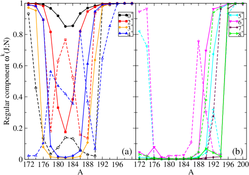
Figure 12: (Color online) Regular content of the two lowest-lying states for each $J$ value (full lines with closed symbols correspond with the first state while dashed lines with open symbols correspond with the second state) resulting from the IBM-CM calculation, as presented in figure 4.

In Fig. 12, we present the weight of the wave functions contained within the $[N]$-boson subspace, defined as the sum of the squared amplitudes $w^{k}(J,N)\equiv\sum_{i}\mid a^{k}_{i}(J;N)\mid^{2}$, for both the yrast states, $(k=1)$, and the $(k=2)$ states (the latter are indicated with a dashed line) for spins $J^{\pi}=0^{+},2^{+},3^{+},4^{+}$ in panel (a) and $J=5^{+},6^{+},7^{+},8^{+}$ in panel (b). The results exhibit an interesting behaviour, both as a function of angular momentum $J$ and as a function of the changing mass number. First, one notices the complementary behaviour of the $0_{2}^{+}$ state as compared to the $0_{1}^{+}$ state. This has important consequences for the study of the hindrance factor for $\alpha$ decay from the Pb ground state into the 0${}^{+}_{1,2}$ states in the Hg nuclei, as will be discussed in Section IV. The $2_{1}^{+}$ and $2_{2}^{+}$ states also present the same complementary behaviour, interchanging their character near mid shell, however with the second $2^{+}$ state becoming of regular character by A=190 and onwards. The $4^{+}_{1}$ state shows a very smooth behavior, almost fully symmetric around A=182, whereas the second $4^{+}$ state shows some more complicated character, which is a consequence of the crossing of a number of rather close-lying $4^{+}$ states when going from nucleus to nucleus (see Fig. 13). The $3_{1}^{+}$ state results to be mainly regular for the lighter and heavier isotopes while mainly intruder at mid shell. The $3_{2}^{+}$ state is not depicted because a rather erratic behaviour shows up which is due to the multiple crossing with other $3^{+}$ states. The higher-spin $5^{+}$, $6^{+}$, $7^{+}$, and $8^{+}$ states are almost pure intruder states along the whole chain except for the lightest and heaviest isotopes. Note that due to the construction of the Hamiltonian for the heavier isotopes, we have imposed by hand that the intruder states should be above $\sim 3$ MeV, forcing the wave function of all these states to have a mainly regular structure.

Table 5: Comparison of the experimental relative B(E2) values with the IBM-CM Hamiltonian results. From left to right we give: isotope, transition, $\gamma$-ray energy, intensity of the transition, multipolarity, experimental relative B(E2) value and the IBM-CM calculations. Data are taken from else11 for ¹⁸⁰Hg , from rapi13 for ^182,184Hg, gutt81 for ^186,188Hg, and korte91 for ¹⁹⁰Hg. We use the expressions $\mbox{B(E2)}=100\times\left(\frac{\mbox{I}_{\gamma}}{\mbox{I}_{\gamma}^{ref}}\right)\times\left(\frac{\mbox{E}_{\gamma}^{ref}}{\mbox{E}_{\gamma}}\right)^{5}$ and $\Delta(\mbox{B(E2)})=\mbox{B(E2)}\times\sqrt{\ \left(\frac{\Delta(\mbox{I}_{\gamma})}{\mbox{I}_{\gamma}}\right)^{2}+\left(\frac{\Delta(\mbox{I}_{\gamma}^{ref})}{\mbox{I}_{\gamma}^{ref}}\right)^{2}}$ in order to extract the relative B(E2) values and their corresponding relative errors.

	Transition	Eγ(keV)	Iγ	Mult.	Exp.	IBM-CM
180Hg	$2_{2}^{+}\rightarrow 0_{2}^{+}$	181.8	0.16(1)	E2	100	100
	$2_{2}^{+}\rightarrow 0_{1}^{+}$	601.6	24.3(12)	E2	38(3)	11
	$4_{1}^{+}\rightarrow 2_{2}^{+}$	104.7	1.4(4)	E2	100	100
	$4_{1}^{+}\rightarrow 2_{1}^{+}$	272.0	54.2(27)	E2	33(9)	272
182Hg	$2_{2}^{+}\rightarrow 0_{2}^{+}$	213.0	1.4(5)	E2	730(260)	554
	$2_{2}^{+}\rightarrow 0_{1}^{+}$	547.8	21.5(8)	E2	100	100
	$4_{2}^{+}\rightarrow 2_{2}^{+}$	576.6	15.0(2)	E2	650(65)	850
	$4_{2}^{+}\rightarrow 2_{1}^{+}$	772.6	10(1)	E2	100	100
184Hg	$2_{2}^{+}\rightarrow 0_{2}^{+}$	159.4	1.7(7)	E2	3500(1400)	2350
	$2_{2}^{+}\rightarrow 0_{1}^{+}$	534.7	20.7(7)	E2	100	100
	$4_{1}^{+}\rightarrow 2_{2}^{+}$	118.8	0.5(3)	E2	250(150)	45
	$4_{1}^{+}\rightarrow 2_{1}^{+}$	287.0	16.7(3)	E2	100	100
	$4_{2}^{+}\rightarrow 2_{2}^{+}$	552.0	9.5(7)	E2	500(50)	346
	$4_{2}^{+}\rightarrow 2_{1}^{+}$	719.6	7.1(4)	E2	100	100
186Hg	$2_{2}^{+}\rightarrow 0_{2}^{+}$	97		E2	$>10^{5}\pm 3\cdot 10^{4}$	24000
	$2_{2}^{+}\rightarrow 0_{1}^{+}$	621		E2	100	100
	$4_{1}^{+}\rightarrow 2_{2}^{+}$	187		E2	210(90)	303
	$4_{1}^{+}\rightarrow 2_{1}^{+}$	402		E2	100	100
	$4_{2}^{+}\rightarrow 2_{2}^{+}$	460		E2	110(20)	130
	$4_{2}^{+}\rightarrow 2_{1}^{+}$	675		E2	100	100
	$6_{2}^{+}\rightarrow 4_{2}^{+}$	597		E2	2900(300)	9500
	$6_{2}^{+}\rightarrow 4_{1}^{+}$	870		E2	100	100
188Hg	$4_{2}^{+}\rightarrow 2_{2}^{+}$	327		E2	8070(580)	2170
	$4_{2}^{+}\rightarrow 2_{1}^{+}$	795		E2	100	100
	$6_{1}^{+}\rightarrow 4_{2}^{+}$	301		E2	270 (20)	97
	$6_{1}^{+}\rightarrow 4_{1}^{+}$	504		E2	100	100
	$6_{2}^{+}\rightarrow 4_{2}^{+}$	569		E2	130(10)	240
	$6_{2}^{+}\rightarrow 4_{1}^{+}$	772		E2	100	100
190Hg	$2_{4}^{+}\rightarrow 0_{2}^{+}$	292	0.03(2)	E2	$6\cdot 10^{4}\pm 4\cdot 10^{4}$	8470∗
	$2_{4}^{+}\rightarrow 0_{1}^{+}$	1571	0.21(12)	E2	100	100
	$4_{2}^{+}\rightarrow 2_{4}^{+}$	404	0.28(8)	E2	19000(6000)	570∗
	$4_{2}^{+}\rightarrow 2_{1}^{+}$	1559	1.22(9)	E2	100	100
	$6_{2}^{+}\rightarrow 4_{2}^{+}$	535	0.75(6)	E2	30700 (3500)	7615∗
	$6_{2}^{+}\rightarrow 4_{1}^{+}$	1468	0.38(3)	E2	100	100

Finally, to explain the sudden changes in the structure of the wave functions, we have to take into account that in most cases several states with identical angular momentum remain approximately at the same excitation energy, but have a different character. So, it can happen that close-lying states interchange character when passing from one isotope to the next one, resulting in an abrupt change in the wave function content. This is depicted in Fig. 13 where we show the energy spectra corresponding to the Hamiltonian given in Table 2, separating the different angular momenta, as a matter of clarity, and distinguishing the character of the states, using i.e., full lines for the regular states ($w^{k}>0.5$) and dashed lines for the intruder ones ($w^{k}<0.5$) (see panels (a) to (e) for $J^{\pi}=0^{+},...,8^{+}$, respectively). Note that the missing points correspond to regular states with an excitation energy which is larger than $\sim 3$ MeV and do not appear within the scale of the figure. We can use this figure to understand the observed behaviour as depicted in Fig. 12. As an illustration we consider the case of the $J^{\pi}=0^{+}$ states: the first excited $0^{+}$ state corresponds to mainly a regular state for A $\sim$ 172, then moves to become an intruder state up to A=190 and finally returns to become the regular ground state up to A=200. The second excited $J^{\pi}=0^{+}$ state is an intruder state at the low-mass region with A $\sim$ 172, then moves to become the first regular state up to A=176, proceeds to be characterized as the second intruder state up to A=188, as first regular state at A=190, as first intruder state (A=192-194) next, to end up as the second regular state (A=196-200).

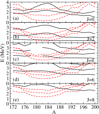
Figure 13: (Color online) Energy systematics for a set of selected states, separated by angular momentum. The full lines denote states with $w^{k}(J,N)>0.5$ (mainly regular) and dashed lines for states with $w^{k}(J,N)<0.5$ (mainly intruder).

In order to understand more clearly the way the energy spectra have been affected by the mixing term, we recalculate the energy spectra using the Hamiltonian presented in table 2, but now switching off the mixing term. The spectra are presented in Fig. 14 where we show the lowest two regular and the lowest intruder state for different angular momenta. One observes a rather flat behavior of the energy for the regular states, but with an up sloping tendence moving to the lighter isotopes. The energy of the intruder states is smoothly decreasing up to neutron mid-shell (minimum occurs at N=102), where it starts increasing again. This effect results mainly from the smooth change of the Hamiltonian parameters when passing from isotope to isotope.

Figure 14: (Color online) Energy spectra for the IBM-CM Hamiltonian presented in table 2, switching off the mixing term. The two lowest-lying regular states and the lowest-lying intruder state for each of the angular momenta are shown (full lines with closed symbols for the regular states while dashed lines with open symbols are used for the intruder states).

A simultaneous analysis of figures 12 and 14, combined with the rules of a simple two-level mixing model, allows us to explain the sudden increase of the regular content for all $J^{\pi}$ values at A=188. Inspecting Fig. 14, one observes the close approach of pairs of regular and intruder states with a given angular momentum, especially in the region around A=188. The mixing term, coupling the regular ($N$) and intruder ($N+2$) configurations, can now result in the interchange of character between the states and therefore in the sudden increase of the regular content of the wave function. For states with $J>4$, the effect is even more dramatic because the unperturbed energy of the intruder configuration always lies below the unperturbed energy of the regular one and as a consequence, the interchange in character with the regular configuration at the point of closest approach is enhanced. Eventually, moving towards A=194, the unperturbed energy of the intruder configurations is moving up and crosses the regular configurations. Therefore, as shown in Fig. 12, from A=194 onwards, the two lowest-lying states for each $J^{\pi}$ value have become regular (N-component, mainly) states.

A most interesting decomposition of the wavefunction is obtained by first calculating the wavefunctions within the N subspace as

$$\Psi(l,JM)^{reg}_{N}=\sum_{i}c^{l}_{i}(J;N)\psi((sd)^{N}_{i};JM)~{},$$ (9)

and likewise for the intruder (or N+2 subspace) as

$$\Psi(m,JM)^{int}_{N+2}=\sum_{j}c^{m}_{j}(J;N+2)\psi((sd)^{N+2}_{j};JM)~{},$$ (10)

defining an “intermediate” basis helle05 ; helle08 . These wave functions correspond to the energy levels shown in Fig.14. This generates a set of bands within the 0p-0h and 2p-2h subspaces, corresponding to the unperturbed bands that are extracted in schematic two-level phenomenological model calculations (as discussed in references  drac88 ; duppen90 ; drac94 ; allat98 ; page03 ; drac04 ; lipska13 ), and indeed correspond to the unperturbed energy levels depicted in Fig. 14.

The overlaps ${}_{N}\langle l,JM\mid k,JM\rangle$ and ${}_{N+2}\langle m,JM\mid k,JM\rangle$ can then be expressed as,

$${}_{N}\langle l,JM\mid k,JM\rangle=\sum_{i}a^{k}_{i}(J;N)c^{l}_{i}(J;N),$$ (11)

and

$${}_{N+2}\langle m,JM\mid k,JM\rangle=\sum_{j}b^{k}_{j}(J;N+2)c^{m}_{j}(J;N+2),$$ (12)

(see expressions (9) and (10)). In Fig. 15 we show these overlaps, but squared, where we restrict ourselves to the first and second state ($k=1,2$) with angular momentum J^π=0⁺,2⁺,3⁺,4⁺,5⁺,6⁺,7⁺,8⁺, and give the overlaps with the lowest three bands within the regular $(N)$ and intruder $(N+2)$ spaces ($l=1,2,3$ and $m=1,2,3$). Since these figures are given as a function of mass number, one obtains a graphical insight into the changing wave function content. In particular, in the upper panel (a), corresponding to the first state of each angular momentum, an inverted parabola separating the regular and the intruder states as a function of increasing angular momentum is clearly observed. In the lower panel (b), the parabolic shape is also present but in this case it does not separate so clearly into regular and intruder configurations. The central region mainly corresponds to the second lowest intruder state while the outer region corresponds to the second regular and the first intruder state.

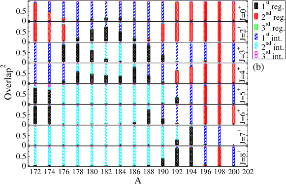
Figure 15: (Color online) Overlap of the wave functions of Eq. (7), with the wave functions describing the unperturbed basis Eq. (9) and Eq. (10). panel (a): overlaps for first $0^{+},2^{+},3^{+},4^{+};5^{+},6^{+},7^{+},8^{+}$ state, panel (b): overlaps for the corresponding second state (see also text).

IV Study of other observables: isotopic shifts and alpha-decay hindrance factors

IV.1 $\alpha$-decay hindrance factors

In the Pb-region, most interesting results were obtained when the content of the nuclear wave functions was tested through $\alpha$-decay measurements. It was shown by Andreyev et al. andrei00 that $\alpha$-decay has been instrumental as a sensitive probe to prove the presence of a triplet of $0^{+}$ states in ¹⁸⁶Pb, each corresponding to a different shape.

Wauters et al. wauters94 ; wauters94a carried out experiments on the $\alpha$-decay from the Po, Pb and Hg nuclei to the Pb, Hg and Pt nuclei, respectively, concentrating in particular on the N=104 mid-shell region. $\alpha$ decay is a highly sensitive fingerprint, precisely because an $\alpha$ particle is emitted in the decay, a process which requires the extraction of two protons and two neutrons from the initial nucleus. The comparison of s-wave l=0 $\alpha$-decay branches from a given parent nucleus (the Pb $0^{+}$ ground state in the present situation) to $0^{+}$ states in the daughter nucleus (the Hg $0^{+}$ ground state and excited $0^{+}$ states) is important in this respect.

Figure 16: A schematic view of the $\alpha$-decay proceeding from the 0⁺ Pb ground state into the 0${}^{+}_{1,2}$ states of the Hg nuclei.

The reduced $\alpha$-decay widths themselves are very difficult to calculate on an absolute scale delion13 , but hindrance factors clearly reflect possible changes amongst the wave functions describing various $0^{+}$ states in a given daughter nucleus duppen00 well (see Garc11 for the precise definition and applications to the Hg to Pt $\alpha$ decay hindrance factor calculations as compared with the data).

These experiments indicated that, in the neutron mid-shell region, the $0^{+}$ ground-state in the Pb and Hg nuclei is essentially consistent with a closed Z=82 core and a two-proton hole configuration in the Z=82 core wauters94 ; wauters94a (see Fig. 16). However, $\alpha$-decay feeding into the first-excited $0^{+}_{2}$ state exhibits a hindrance factor. The specific values of the hindrance factors are the adopted values as given in Nuclear Data Sheets, starting from the original data wauters94 ; wauters94a . This is qualitatively in line with the results presented in Fig. 12, where the $0^{+}_{1}$ ground state mainly consists of the regular $[N]$ configuration, dropping to a value of $\approx 85\%$ of the $[N]$ component at A=$182,184$. The results of the present calculation indicate an almost symmetric structure with respect to the mid-shell N=104 neutron number. The important point here, as also stressed by Van Duppen and Huyse duppen00 , is the consistent picture that results when treating the Po, Pb, Hg, and Pt nuclei jointly. It turns out that the structure of the wavefunctions for the 0${}^{+}_{1}$ and 0${}^{+}_{2}$ states are consistent with the wavefunctions extracted from both $\alpha$-decay hindrance factors and E0 transitions between the ground and first excited 0⁺ states delion95 ; richards97 ; wood99 ; joshi94 .

IV.2 Isotopic shifts

Experimental information about ground-state charge radii is also available for both the even-even and odd-mass Hg nuclei. Combined with similar data for the adjacent Po, Pb, and Pt nuclei, as well as for the odd-mass Bi, Tl and Au nuclei, the systematic variation of the charge radii supplies invaluable information on the ground-state wave function otten89 ; kluge03 . We illustrate the relative changes defined as $\Delta{\langle r^{2}\rangle}_{A}\equiv\langle r^{2}\rangle_{A+2}$ -$\langle r^{2}\rangle_{A}$ in Fig. 17 (left side) and the overall behaviour of ${\langle r^{2}\rangle}_{A}$ relative to the radius at mass A=198 in Fig. 17 (right side). The experimental data are taken from Ulm et al. ulm86 .

To calculate the isotope shifts, we have used the standard IBM-CM expression for the nuclear radius

$$r^{2}=r_{c}^{2}+\hat{P}^{{\dagger}}_{N}(\gamma_{N}\hat{N}+\beta_{N}\hat{n}_{d})\hat{P}_{N}+\hat{P}^{{\dagger}}_{N+2}(\gamma_{N+2}\hat{N}+\beta_{N+2}\hat{n}_{d})\hat{P}_{N+2}.$$ (13)

The four parameters appearing in this expression are adjusted to the experimental data. Note that only the experimental values past mid shell (A=184) are used. The resulting values are $\gamma_{N}=-0.099$ fm², $\beta_{N}=0.004$ fm², $\gamma_{N+2}=-0.059$ fm², and $\beta_{N+2}=0.013$ fm² and are only valid for the second half of the shell.

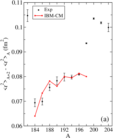
Figure 17: (Color online) Panel (a): Isotopic shift for the Hg nuclei. Panel (b): Charge mean-square radii for the Hg nuclei. The data are taken from ulm86 .

The panel (a) of Fig. 17 shows a relatively small variation of the isotopic shift over the whole chain of the Hg isotopes (184 $\leq$ A $\leq$ 204). However, two different regions are clearly marked: one region from A=184 to A=196 in which a steady increase of the isotopic shift is observed ending in a smooth stabilization at A = 196, followed by the region from A=198 to A=204 where a sudden increase in the isotopic shift occurs, suggesting the transition into a new regime. The mean-square charge radius exhibits (see panel (b) of Fig. 17) a smooth decrease from A=204 down to A=184, but exhibits systematic deviations from the linear trend, which is marked with the dotted straight line. These data suggest that no major change in the ground-state structure appears along the whole chain of the Hg isotopes, contrary to what is observed in the odd-mass isotopes otten89 ; kluge03 (and cf. Fig. 21 in Ref. heyde11 ).

The IBM-CM exhibits quantitative agreement up to A=196. For A=198, a too small theoretical value is obtained as compared with the data, where one observes a change to a significantly larger value of the isotopic shift which tends to flatten at A= 204. It is a remarkable fact that the overall variation of the isotopic shifts along the whole isotopic Hg chain is very small $\approx 0.05$ fm², and this range is fairly well reproduced by the IBM-CM calculations. This is in contrast with the Pt isotopes in which the overall variation amounts to $\approx 0.2$ fm²  Garc11 . Therefore, the good reproduction of this range confirms the calculated interplay between the $[N]$ and $[N+2]$ contributions in the $0^{+}$ ground state wave function along the whole chain of Hg isotopes.

V The connection of the IBM-CM and the mean field studies

V.1 Mean-field studies: phenomenological potentials and self-consistent methods

The Hg nuclei have been studied using mean-field methods emphasizing the intrinsic structure of atomic nuclei bender03 . A more phenomenological approach, within the same spirit, has been used to study the Hg nuclei (and nuclei in the Pb region taken more generally) starting from a deformed Woods-Saxon (DWS) potential as an approximation to a deformed mean-field. We stress the fact (see discussion further on) that the intrinsic property such as an oblate and prolate shape, or, more generally, a shape defined over the $\beta,\gamma$ domain, is not an observable and its use to confront them with data only serves as a qualitative guide. A clean separation of shapes, which has been shown through extensive experimental studies in the Pb nuclei, leads to good evidence for the coexistence of spherical, oblate and prolate shapes. However, moving away from the Pb nuclei, into the Hg, Pt and Po, Rn nuclei, much stronger mixing is expected and, as such, a discussion starting from the intrinsic frame, at lowest order, can only be a starting point.

Concentrating on the Hg nuclei, the total energy has been calculated starting from a deformed Woods-Saxon potential (DWS) bengt87 ; naza93 . The results give rise to spherical shapes up to A=176, followed by a region where a slightly oblate shape ($\beta\sim$ -0.13 to -0.10) and a prolate shape ($\beta\sim$ 0.20 to 0.25) for 178 $\leq$ A $\leq$ 188, coexist, changing into oblate shapes only from mass A=190 onwards, ending in a spherical shape at A=200. These studies are restricted to axial systems. In a number of papers, the obvious point is made to associate the calculated prolate-oblate energy difference $\Delta E_{po}=E_{prolate}-E_{oblate}$ with the experimental energy difference $\Delta E_{x}=E_{x}(0^{+}_{2})-E_{x}(0^{+}_{1}$). In those cases when strong mixing is involved, however, it can become unsafe to use this approach in order to decide on a given character of “observed” states as corresponding to prolate and/or oblate states.

The early mean-field calculations of Girod and Reinhard girod82 , using axial quadrupole deformation presented very much the same outcome with respect to shape coexistence in the interval 180 $\leq$ A $\leq$ 188. Covering the full $\beta,\gamma$ plane, Delaroche et al. dela94 showed the appearance of shape coexistence in the 184 $\leq$ A $\leq$ 188 isotones, with clear indications for triaxal bands in A=188.

Relativistic-mean-field calculations, with specific application to the Hg nuclei, using the NL1 effective interaction patra94 ; yoshida94 resulted in both serious overbinding for these nuclei and moreover indicated that the lowest energy in the 178$\leq$A$\leq$188 mass region was associated with a prolate shape, contrary to the non-relativistic calculations girod82 ; dela94 . Using a different treatment of the pairing energy, this time the lowest energy obtained corresponded with an oblate shape yoshida97 . The problem here is that on the scale of total binding energies, differences with the data as large as $\sim$10 MeV resulted, with a value for $\Delta E_{po}$ of $\sim$0.5 MeV only, which makes this result very sensitive to the precise prescription used. Niksic et al. niksic02 made a thorough study aiming to construct an effective interaction, called NL-SC. The constraint was to reproduce as well as possible the experimental gap in the proton single-particle spectrum, as this quantity is of major importance in deriving correctly the energy cost to create np-mh excitations across the Z=82 closed shell. With this force, called NL-SC, both the total binding energy and charge radii for the Hg nuclei were reproduced rather well. Moreover, as was the case with the DWS calculations, the oblate minimum becomes the lowest in the 178$\leq$A$\leq$188 region.

It is interesting to point out that most recent mean-field total energy calculations, either starting from the Gogny D1M force nomura12a or from the Skyrme SLy6 force yao13 result in the prolate energy minimum being the lowest (even after projecting on angular momentum J in the latter case) from ¹⁸⁰Hg up to ¹⁸⁶Hg (with the oblate and prolate minima becoming very close at mass A=186 in the former). In the latter calculation, Yao et al. yao13 have moved beyond the mean-field, using the constraint of axial symmetry, and calculated the observables so as to confront the theoretical approach with the genuine data set (which they did for the Pb and Po nuclei, as well). In both calculations, the oblate minimum remains the only one, once having reached A=190 and beyond. What becomes clear is that collective dynamical correlations determine the final outcome of the nuclear properties, definitely in the case of the Hg nuclei where the oblate and prolate minima in the region 178$\leq$A$\leq$188 are quite close, resulting in a shallow energy surface yao13 along the triaxial quadrupole deformation, indicating the need for GCM calculations covering the full $\beta,\gamma$ plane.

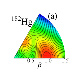
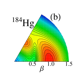
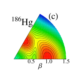
Figure 18: (Color online) Matrix coherent-state calculation for ^182-186Hg, corresponding with the present IBM-CM Hamiltonian (table 2). The energy spacing between adjacent contour lines equals $100$ keV and the deepest energy minimum is set to zero, corresponding to the red color.

V.2 Mean-field approximation to the IBM: the energy surfaces

A geometric interpretation of the IBM can be constructed using the intrinsic state formalism, as proposed in the 1980’s by Bohr and Mottelson Bohr80 , Ginocchio et al. gino80 and by Dieperink et al. diep80a ; diep80b , based on the concept of coset spaces gil74 . This provides a simple way to connect with the intrinsic geometric mean-field properties of the model and therefore to obtain a simple picture of the shape of the nuclei.

To define the intrinsic state, one assumes that the dynamical behavior of the system can be described using independent bosons (“dressed bosons”) moving in an average field Duke84 . The ground state of the system is a condensate $|N;\beta,\gamma\rangle$ of bosons, occupying the lowest–energy phonon state, $\Gamma^{\dagger}_{c}$,

$$|N;\beta,\gamma\rangle={1\over\sqrt{N!}}(\Gamma^{\dagger}_{c})^{N}|0\rangle,$$ (14)

where

$$\Gamma^{\dagger}_{c}={1\over\sqrt{1+\beta^{2}}}\left(s^{\dagger}+\beta\cos\gamma\,d^{\dagger}_{0}+{1\over\sqrt{2}}\beta\sin\gamma\,(d^{\dagger}_{2}+d^{\dagger}_{-2})\right),$$ (15)

and $\beta$ and $\gamma$ are variational parameters related with the shape variables in the geometrical collective model bomot75 . The expectation value of the Hamiltonian in the intrinsic state (14) provides the energy surface of the system, $E(N,\beta,\gamma)=\langle N;\beta,\gamma|\hat{H}|N;\beta,\gamma\rangle$ and the values of $\beta$ and $\gamma$, which minimize the expectation value of the energy, represent the shape of the nucleus. The energy surface obtained in this way is equivalent, up to a scale factor, to the one derived from mean field theory  bender03 . The IBM value of $\gamma$ is directly comparable with the mean field value nomura08 ; nomura10 ; nomura11a ; nomura11b ; nomura13 ; nomura12a , while $\beta$ should be rescaled gino80 .

To analyze the nuclear geometry in the case of IBM-CM, the intrinsic state formalism should be extended. This extension was recently proposed by Frank et al., introducing a matrix coherent-state method Frank02 ; Frank04 ; Frank06 ; Mora08 that allows to describe shape coexistence in a geometric way.

The way to proceed is to define a model space with the states $|N;\beta,\gamma\rangle$, $|\ N+2;\beta,\gamma\rangle$ and to diagonalize the Hamiltonian (1). So, one needs to construct the $2\times 2$ matrix:

$$H_{CM}=\left(\begin{array}[]{cc}E_{N}(N,\beta,\gamma)&\Omega(\beta)\\ \Omega(\beta)&E_{N+2}(N+2,\beta,\gamma)+\Delta^{N+2}\end{array}\right),$$ (16)

in which $E(N,\beta,\gamma)=\langle N;\beta,\gamma|\hat{H}|N;\beta,\gamma\rangle$, $E(N+2,\beta,\gamma)=\langle N+2;\beta,\gamma|\hat{H}|N+2;\beta,\gamma\rangle$, and $\Omega(\beta)=\langle N;\beta,\gamma|\hat{H}|N+2;\beta,\gamma\rangle$. The terms $E_{N}(N,\beta,\gamma)$ and $E_{N+2}(N+2,\beta,\gamma)$ only contain the $N$ and the $N+2$ contributions of the Hamiltonian (1), respectively, while $\Omega(\beta)$ corresponds to the matrix element of the mixing term $\hat{V}_{\rm mix}^{N,N+2}$. Note that $\Omega(\beta)$ only depends on $\beta$, while $E_{N}(N,\beta,\gamma)$ and $E_{N+2}(N+2,\beta,\gamma)$ depend on $\beta$ and $\gamma$. The explicit expressions of these matrix elements (see ref. Mora08 ) are:

$$E_{i}(N_{i},\beta,\gamma) = (\varepsilon_{i}+6\kappa^{\prime}_{i})\frac{N_{i}\beta^{2}}{1+\beta^{2}}+\kappa_{i}\left(\frac{N_{i}}{1+\beta^{2}}(5+(1+\chi_{i}^{2})\beta^{2})+\frac{N_{i}(N_{i}-1)}{(1+\beta^{2})^{2}}\right.$$ (17)

$$\times \left.\big{(}\frac{2}{7}\chi_{i}^{2}\beta^{4}-4\sqrt{\frac{2}{7}}\chi_{i}\beta^{3}\cos{3\gamma}+4\beta^{2}\big{)}\right),$$

$$\Omega(\beta) = \frac{\sqrt{(N_{i}+2)(N_{i}+1)}}{1+\beta^{2}}\left(w_{0}^{N,N+2}+w_{2}^{N,N+2}\frac{\beta^{2}}{\sqrt{5}}\right).$$ (18)

To obtain the energy surface one has to diagonalize (16) and to consider the lowest eigenvalue. The meaning of the higher eigenvalue is not yet fully understood and will not be used along this paper.

Since its introduction, the intrinsic state formalism for IBM-CM Hamiltonians has been used in very few cases Frank06 ; Mora08 ; nomura12a ; gar13_unpu , however it can provide complementary information to the results from the IBM-CM in the laboratory frame, in particular about the energy surface and the shape of the nucleus. This is very useful in order to compare the energy surface, here starting from a lab frame formulation (the IBM), with the total energy calculated using self-consistent HFB mean field methods.

Figure 19: Axial-symmetric energy curves for ^182-186Hg using the matrix coherent-state calculation.

We have calculated the energy surfaces of the whole chain of Hg isotopes, ^172-200Hg, however a full analysis will be presented elsewhere gar13_unpu . In this section, we focus on the particular cases of ¹⁸²Hg, ¹⁸⁴Hg, and ¹⁸⁶Hg which are at the mid shell and have been analyzed in detail in yao13 through a beyond mean-field HFB calculation. In Fig. 18 (panels (a), (b), and (c)) we present the energy surface of ^182-186Hg in the $\beta-\gamma$ plane, while in Fig. 19 we depict the axial-symmetric energy curves for the three isotopes. Moreover, as a complementary view, we depict in Fig. 20 the three-dimensional energy plot of ¹⁸⁴Hg. These figures show that the region around the minima is rather shallow in both the $\beta$ and $\gamma$ directions. Inspecting the energy curves along the axial line only, the three nuclei correspond to prolate shapes although in ¹⁸⁶Hg the minima are almost degenerate. However, in these three cases there are prolate and oblate minima connected by a path characterized by a much lower barrier (see Fig. 20). In Ref. yao13 , using the Skyrme Sly6 force, the HFB energy surface in the $\beta-\gamma$ plane for ¹⁸⁴Hg is shown. That figure is equivalent, up to a scale factor in $\beta$, to the IBM-CM results. Moreover the axial energy curves are also very similar to the IBM-CM results. In both approaches the three nuclei are prolate, up to the mean-field level, but due to the flat behavior of the energy surface there is not a clear-cut preference for a dominant oblate nor prolate shape characterizing these nuclei. Indeed, as can be observed in Fig. 19 (panels (a), (b), and (c)), the prolate and the oblate minima - which are real minima and not saddle points - are almost degenerate in energy and although there is a large barrier at the spherical shape, a rather flat path connects both minima going through the triaxial region. Therefore, in order to make the step towards the observable properties, there is the need to include the quadrupole collective dynamics, either restricting to axial symmetry or extending into the full triaxial $\beta-\gamma$ plane, and go beyond mean field.

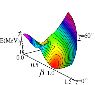
Figure 20: (Color online) Three dimension energy plot for ¹⁸⁴Hg using the matrix coherent-state calculation.

V.3 The quadrupole invariants

The IBM can provide us with both the energy spectrum, the corresponding wave functions as well as all derived observables (B(E2)’s, quadrupole moments, radii,…), working within the lab frame, as well as the corresponding mean-field energy surface, defining a nuclear shape over the $\beta,\gamma$ intrinsic frame. Even though the shape of the nucleus is not an experimental observable, it is still possible to extract from the data direct information about various moments characterizing the nuclear shape corresponding with a given eigenstate. Using Coulomb excitation, it is possible to extract the most important diagonal and non-diagonal quadrupole and octupole matrix elements, including their relative signs and, in a model independent way, extract information about nuclear deformation as shown by Kumar, Cline and co-workers kumar72 ; Cline86 ; Wu96 ; clement07 ; sreb11 .

The essential point is the introduction of an “equivalent ellipsoid” view of a given nucleus  kumar72 corresponding to a uniformly charged ellipsoid with the same charge, $\langle r^{2}\rangle$, and E2 moments as the nucleus characterized by a specific eigenstate kumar72 ; wood12 .

From the theoretical point of view the nuclear shape can be calculated using the quadrupole shape invariants. They correspond to:

$$q_{2,i} = \sqrt{5}\langle 0_{i}^{+}|[\hat{Q}\times\hat{Q}]^{(0)}|0_{i}^{+}\rangle,$$ (19)

$$q_{3,i} = -\sqrt{\frac{35}{2}}\langle 0_{i}^{+}[\hat{Q}\times\hat{Q}\times\hat{Q}]^{(0)}|0_{i}^{+}\rangle.$$ (20)

Note that these observables can be calculated for any $0_{i}^{+}$ state but to simplify the notation we do not write explicitly the index $i$. For the triaxial rigid rotor model wood09 they are directly connected with the deformation parameters,

$$q_{2} = q^{2},$$ (21)

$$q_{3} = q^{3}\cos{3~{}\delta},$$ (22)

where $q$ denotes the nuclear intrinsic quadrupole moment and $\delta$ the triaxial degree of freedom,

$$q = \sqrt{q^{2}},$$ (23)

$$\delta = \frac{60}{\pi}\arccos{\frac{q_{3}}{q_{2}^{3/2}}}.$$ (24)

The value of $\delta$ is equivalent, up to first-order approximation, to the value of $\gamma$ appearing in section V.2 (see Ref. Srebrny06 for further details).

Table 6: Quadrupole shape invariants for the ^180-200 Hg isotopes. Experimental values are taken from lipska13 .

Isotope	State	$q^{2}$ (e2b2)		$\cos 3~{}\delta$		$\delta$ (deg)
		Theo.	Exp.	Theo.	Exp.	Theo.	Exp.
$180$	$0_{1}^{+}$	$1.83$	-	$-0.01$	-	$30.3$	-
	$0_{2}^{+}$	$6.54$	-	$0.63$	-	$17.0$	-
$182$	$0_{1}^{+}$	$2.00$	$2.02(_{-15}^{+16})$	$0.23$	$-1.33(_{-87}^{+109})$	$25.5$	$(35,60)$
	$0_{2}^{+}$	$6.19$	$9.7(_{-51}^{+74})$	$0.65$	$0.58(_{-61}^{+98})$	$16.6$	$18(_{-18}^{+13})$
$184$	$0_{1}^{+}$	$2.08$	$1.66(12)$	$-0.08$	$-1.04(_{-46}^{+42})$	$31.5$	$(43,60)$
	$0_{2}^{+}$	$5.40$	$13.9(_{-69}^{+97})$	$0.54$	$-0.34(_{-36}^{+34})$	$19.2$	$37(_{-7}^{+8})$
$186$	$0_{1}^{+}$	$1.45$	$1.56(_{-25}^{+23})$	$-0.13$	-	$32.6$	-
	$0_{2}^{+}$	$6.07$	-	$0.60$	-	$17.7$	-
$188$	$0_{1}^{+}$	$1.77$		$-0.20$		$33.9$
	$0_{2}^{+}$	$5.62$	-	$0.59$	-	$18.0$	-
$190$	$0_{1}^{+}$	$1.48^{*}$	-	$-0.19^{*}$	-	$33.7^{*}$	-
	$0_{2}^{+}$	$4.78^{*}$	-	$-0.03^{*}$	-	$30.7^{*}$	-
$192$	$0_{1}^{+}$	$1.11^{*}$	-	$-0.24^{*}$	-	$34.6^{*}$	-
	$0_{2}^{+}$	$0.87^{*}$	-	$-0.38^{*}$	-	$37.5^{*}$	-
$194$	$0_{1}^{+}$	$0.91^{*}$	-	$-0.16^{*}$	-	$33.1^{*}$	-
	$0_{2}^{+}$	$0.67^{*}$	-	$-0.19^{*}$	-	$33.7^{*}$	-
$196$	$0_{1}^{+}$	$1.14^{*}$	-	$-0.13^{*}$	-	$32.5^{*}$	-
	$0_{2}^{+}$	$0.74$	-	$-0.39$	-	$37.7$	-
$198$	$0_{1}^{+}$	$0.97$	-	$-0.29$	-	$35.5$	-
	$0_{2}^{+}$	$0.57$	-	$-0.57$	-	$41.7$	-
$200$	$0_{1}^{+}$	$0.87$	-	$-0.79$	-	$47.3$	-
	$0_{2}^{+}$	$0.64$	-	$-0.87$	-	$50.3$	-

To calculate analytically the quadrupole shape invariants characterizing the nucleus in its ground-state and low-lying excited states, it is necessary to resort to a closure relation, $\textbf{1}=\sum_{J,i,M}|J_{i}M\rangle\langle J_{i}M|$,

$$q_{2,i} = \sum_{r}\langle 0_{i}^{+}||\hat{Q}||2_{r}^{+}\rangle\langle 2_{r}^{+}||\hat{Q}||0_{i}^{+}\rangle,$$ (25)

$$q_{3,i} = -\sqrt{\frac{7}{10}}\sum_{r,s}\langle 0_{i}^{+}||\hat{Q}||2_{r}^{+}\rangle\langle 2_{r}^{+}||\hat{Q}||2_{s}^{+}\rangle\langle 2_{s}^{+}||\hat{Q}||0_{i}^{+}\rangle.$$ (26)

Calculations of quadrupole shape invariants were carried out before within the framework of the IBM by Jolos et al. Jolo97 and later by Werner and coworkers in Ref. Werner00 .

A comparison with the experimental values can be carried out whenever a large enough set of reduced E2 matrix elements can be extracted from, e.g., Coulomb excitation experiments (see Cline86 ; Wu96 for a discussion on the determination of the relative signs of these reduced E2 matrix elements). Such a comparison constitutes a very stringent test for the theoretical model and, at the same time, provides a clear picture of the nuclear shape. In table 6 we provide the theoretical values for the quadrupole shape invariants for all the nuclei where it has been possible to fix the effective charges and we also compare with the available experimental data.

In table 6, we compare our results with recent Coulomb excitation experiments of ^182-188Hg at REX-ISOLDE and Miniball, allowing to extract a useful set of reduced E2 matrix elements  lipska13 . It turns out that our IBM-CM calculations indeed give rise to values of $q^{2}$ that differ by a factor of $\approx$ 3 between the $0^{+}_{1}$ and $0^{+}_{2}$ states. The calculated values are particularly stable, independent of the mass number A=182-188 whereas the experimental data seem to indicate an increasing deformation value with increasing A. Evaluating the invariant $q^{3}\cos(3\delta)$ requires a lot more matrix elements imposing restrictions in the summation over the possible intermediate states. This will be particularly important for the $0^{+}_{2}$ state as one can expect still important matrix elements connecting to higher-lying $2^{+}_{i}$ states (even up to $i=4$). Here, our calculated values do not show a particular correlation with the experimentally extracted values for $\langle\cos(3\delta)\rangle$.

We have investigated the convergence in the summation over the intermediate basis and found that in the four nuclei studied, i.e., ^182-188Hg, the summation is particularly sensitive to the number of $2^{+}_{i}$ states included. To exemplify this effect, we focus on the nucleus ¹⁸⁴Hg. According to Eqs. (25)-(26), used to calculate the value of $q_{2,i}$ and $q_{3,i}$, it is not known how many matrix elements will have to be included to reach a convergent result. One could expect the matrix elements to rapidly fall (becoming vanishingly small) with increasing excitation energy of the $2^{+}_{i}$ states involved. Therefore, one could expect that the sum can safely be truncated, retaining only very few terms. We show the effect of the number of states on the deformation parameters in table 7 concerning the variation of $q^{2}$ and of $\cos{3\delta}$ for the $0_{1}^{+}$ and $0_{2}^{+}$ states, as a function of the number of $2^{+}_{i}$ states in the sum. One notices that in order to obtain a stable value for $\cos{3\delta}$, one needs to include more $2^{+}$ states than is the case for $q^{2}$. One also notices that convergence sets in faster for the $0^{+}_{1}$ state as compared to the $0^{+}_{2}$, at least in the case of $q^{2}$. Particularly striking is the change in sign of $\cos{3\delta}$ for the $0_{1}^{+}$ state, when increasing the number of intermediate $2^{+}$ states from one to two (in the calculation) and, considering up to five intermediate $2^{+}$ states, and oscillation sets in.

Table 7: Calculated value of $q^{2}$ and $\cos{3\delta}$ for the $0_{1}^{+}$ and $0_{2}^{+}$ states in ¹⁸⁴Hg, as a function of the number of $2^{+}$ states included, up to five. The exact value is also given.

$q^{2}$ (e2b2)
$i$	1	2	3	4	5	Exact
$0_{1}^{+}$	1.93	2.03	2.03	2.04	2.06	2.08
$0_{2}^{+}$	2.25	4.71	5.33	5.36	5.39	5.40
$\cos{3\delta}$
$i$	1	2	3	4	5	Exact
$0_{1}^{+}$	0.41	-0.13	-0.15	-0.15	-0.08	-0.08
$0_{2}^{+}$	0.38	1.03	0.51	0.52	0.54	0.54

VI Conclusions

Shape coexistence is a phenomenon that has become a major characteristic of atomic nuclei, all through the nuclear mass table: ranging from the light doubly-closed shell nuclei such as ¹⁶O,⁴⁰Ca, up to heavy nuclei with a large neutron excess such as the Sn (Z=50) and Pb (Z=82) isotopes. In almost all cases, it was the presence of unexpectedly low-excitation energy for $0^{+}$ states, quite often acting as the band-head of an intrinsic structure corresponding with a much larger collectivity as compared to the regular low-lying states. In a number of cases, this even gave rise to highly-correlated states that “inverted” with the less-correlated spherical states such as the so-called islands of inversion.

It has become clear that the presence of low-lying $0^{+}$ states delineates regions where different structures sometime coexist, but depending on the proximity and their mutual coupling, give rise to important mixing thereby sometimes masking the presence of two (or more) structures.

In many cases, it has often been the case that the experimental energy difference between the $0^{+}_{1}$ ground state and a low-lying intruding $0^{+}_{2}$ state was taken as a measure of the energy difference between energy minima associated with oblate and prolate energy surfaces in a mean-field context. It can be concluded though, in part based on the experimental observation of energy spectra and E2 properties for low-lying states $0^{+},2^{+},4^{+}$, that such a relation is not well founded. A first point is the fact that the total energy corresponding with a given nuclear quadrupole shape, at the mean field level, is not an observable. It is only after including all correlations from (i) restoring the symmetries broken in the intrinsic frame going back to a lab frame (making states of good angular momentum J), and, (ii) originating from mixing the mean-fields at various deformations (beyond mean-field calculations) that a comparison between observables such as excitation energies, B(E2) values, …, with theoretical studies becomes possible. This last step can seriously modify the outcome at a purely mean-field level rodri00

In the present study, we have started from a formulation which aims at reducing the huge shell-model spaces occurring in the Pb region when treating proton multi-particle multi-hole excitations across the Z=82 closed shell, jointly with the open neutron shell N=82-126, using the interacting boson model symmetry-dictated approximation (IBM). This approach keeps the essential high and low multipoles of the nuclear effective interaction, i.e., the pairing and quadrupole correlations within a boson model space.

We have analyzed in detail the even-even Hg nuclei in the region 172 $\leq$ A $\leq$ 200, in particular concentrating on the shape coexisting phenomena observed in the 180 $\leq$ A $\leq$ 188,190 region. The IBM, including the configuration mixing between configurations consisting of a closed proton shell at Z=82 and proton 2p-2h excitations across Z=82 (IBM-CM) has been used to describe both energy spectra as well as E2 properties: both absolute and relative B(E2) ratios.

The results show that, in particular at the level of the $2^{+},4^{+}$ states (in the interval 180 $\leq$ A $\leq$ 188), the IBM-CM is able to correctly describe the changing mixing pattern between these two types of configurations. This is particularly the case in order to describe the $2^{+}_{1}$ to $2^{+}_{2}$ energy spacing and its variation as a function of mass number A. For the higher-spin part (J=$8^{+},10^{+}$,…), the difference in character as intruder states versus a regular one is evidenced when comparing energy spectra at a given neutron number, e.g., N=106 for various isotones (Yb up to Hg), as illustrated in figure 5 of  Garc11 . We have carried out a detailed study of the configuration mixing and the resulting wave function content as a function of mass number A. We also point out that studies of $\alpha$-decay hindrance factors and the mean-square charge radii $\langle r^{2}\rangle$ for the ground state, indicate a maximal admixture of 20% in the interval 180 $\leq$ A $\leq$ 200.

Using the coherent-state formalism, we have extracted the mean-field energy corresponding with the IBM-CM approach (the latter formulated in the lab system) which should correspond to the intrinsic energy obtained with a geometric nuclear shape defined over the full quadrupole deformation ($\beta-\gamma$ plane). This allows us to compare with self-consistent mean-field calculations. Our conclusions at this point were surprising. Very much in line with recent mean-field calculations for the Hg nuclei nomura13 ; yao13 where the prolate energy minimum is the deepest one for 176 $\leq$ A $\leq$ 186, as compared to the oblate energy minimum (with the prolate energy minimum disappearing above A=188), the IBM-CM results also in the prolate energy minimum becoming the lowest one for 180 $\leq$ A $<$ 186, being degenerate with the oblate one in A=186 and moving quickly away for A $>188$. These results and the observed correspondences point towards an equivalence at the level of a mean-field description. However, it appears that the dynamics involved in the IBM-CM are able to result in a set of observables that are overall consistent with the large set of experimental data obtained in the Hg nuclei.

We also stress the fact that starting from the experimental data, even though direct information on deformation properties is not present in excitation energies, B(E2) values, branching ratios, E2 matrix elements, it is possible to construct so-called quadrupole invariants by making appropriate sums over the reduced E2 matrix elements. These quadrupole invariants $q_{2}$ and $q_{3}$ need a large enough set of E2 matrix elements that have recently been extracted for the A=$182,184,186$ (partly for A=188) at the Miniball set up at REX-ISOLDE. Our IBM-CM results indicate a large difference in the value of $q_{2}$ for the ground state $0^{+}_{1}$ state ( $\approx 2.0-1.6$ e²b²) as compared to the value derived for the $0^{+}_{2}$ state ($\approx$6 $e^{2}b^{2}$), with the experimental data showing even larger values of $q_{3}$ for the $0^{+}_{2}$ state. In contrast to the experimental data concerning the $q_{3}$ invariant, which is a measure of the non-axial structure of the nuclear shape for a given nuclear eigenstate, and is indicative for having an oblate shape in the ground state for A $=182,184$ and A=188, our IBM-CM results are not so conclusive.

It may be appropriate to overlook the results that have been obtained in the study of shape coexistence within the context of a symmetry-dictated truncation of the shell model, i.e., the IBM-CM passing from the Z=82 closed shell Pb nuclei, over the Hg nuclei into the Pt nuclei. Whereas in the first two series of isotopes, shape coexistence shows up clearly at the level of energy spectra, substantiated by the large experimental efforts to disentangle finer details in the wave functions via measurements of charge radii, lifetime measurements, in-beam spectroscopy, etc, the Pt nuclei are exhibiting, at first sight, a single collective structure. It looks like the coupling between different families (0p-0h and 2p-2h excitations across Z=82, or, spherical, oblate and prolate shapes in a mean-field approach) in the Pb nuclei is rather moderate and only shows up at the lower end of the two bands. The same mixing phenomenon appears to ’disturb’ the presence of two pure sets of configurations in the Hg nuclei, this time particularly at the level of the $2^{+}$ states with rather moderate mixing at the level of the $0^{+}$ states. The behavior in the excitation energy of the two close-lying $2^{+}$ states, however, is changing albeit in a rather smooth way, somehow concealing the configuration mixing. This latter feature becomes dominant in the Pt nuclei where the mixing occurs at the level of the $0^{+}$ state and results in a rather low-lying excited $0^{+}$ state with a particular mass dependence of its excitation energy.

VII Acknowledgment

We are very grateful to Katarzyna Wrzosek-Lipska, Elisa Rapisarda and Liam Gaffney for generous sharing of their most recent results on Coulomb excitation (A=182-188), $\beta$-decay results for A=182 and A=184 and new lifetime data for A=184 and A=186. We thank M. Huyse, P.Van Duppen for continuous interest in this research topic and J.L. Wood for stimulating discussions in various stages of this work and his diligence to quote from his unpublished notes. Financial support from the “FWO-Vlaanderen” (KH and JEGR) and the InterUniversity Attraction Poles Programme - Belgian State - Federal Office for Scientific, Technical and Cultural Affairs (IAP Grant No. P7/12, is acknowledged. This work has also been partially supported by the Spanish Ministerio de Economía y Competitividad and the European regional development fund (FEDER) under Project No. FIS2011-28738-C02-02, by Junta de Andalucía under Project No. FQM318, and P07-FQM-02962, and by Spanish Consolider-Ingenio 2010 (CPANCSD2007-00042).

References

- (1) A. Bohr, B.R. Mottelson, Nuclear structure Vol. II, W.A. Benjamin Inc. Advanced Book Program Reading Massachusetts (1975).
- (2) D.J. Rowe, and J. L. Wood, Fundamentals of Nuclear Models: Foundational Models, World. Scient. Publ. (2010).
- (3) E. Epelbaum, H.-W. Hammer, and U. Meissner, Rev. Mod. Phys. 81, 1773 (2009).
- (4) R. Machleidt, and R. R. Entem, Phys. Repts. 503 1 (2011).
- (5) E. Caurier and G. Martínez-Pinedo and F. Nowacki and A. Poves and A. P. Zuker, Rev. Mod. Phys. 77, 427 2005.
- (6) M. Bender, P.-H. Heenen, and P.-G. Reinhard, Rev. Mod. Phys. 75, 121 (2003).
- (7) D. J. Dean, and M. Hjorth-Jensen, Rev. Mod. Phys. 75, 607 (2003).
- (8) H. Morinaga, Phys. Rev. 101 254 (1956).
- (9) R. Julin, K. Helariutta, and M. Muikku, J. Phys. G 27, R109 (2001).
- (10) G. Neyens, Rep. Progr. Phys. 66, 633 (2003).
- (11) K. Blaum, J. Dilling, and W. Nörtershäuser, Nobel Symposium 152: Physics with Radioactive Beams, eds. C. Fahlander, and B. Jonson, Phys. Scr. T 152 014017 (2013).
- (12) A. Gade, and Th. Glasmachter, Progr. Part. Nucl. Phys. 60, 161 (2008).
- (13) A. Görgen, J. Phys. 37, 103101 (2010).
- (14) T. Baumann, A. Spyrou, and M. Thoennessen, Rep. Progr. Phys. 75, 036301 (2012).
- (15) Y. Blumenfeld, T. Nilsson, and P. Van Duppen, Nobel Symposium 152: Physics with Radioactive Beams, eds. C. Fahlander, and B. Jonson, Phys. Scr. T 152 014023 (2013).
- (16) K. Heyde, P. Van Isacker, M. Waroquier, J.L. Wood, and R.A. Meyer, Phys. Rep. 102, 291 (1983).
- (17) J.L. Wood, K. Heyde, W. Nazarewicz, M. Huyse, and P. Van Duppen, Phys. Rep. 215, 101 (1992).
- (18) K. Heyde and J.L. Wood, Revs. Mod. Phys. 83, 1467 (2011).
- (19) B. R. Barrett, P. Navratil, and J. P. Vary, Progr. Part. Nucl. Phys. 69 131 (2013).
- (20) S. K. Bogner, R. J. Furnstahl, and A. Schwenk, Progr. Part. Nucl. Phys. 65 94 (2010).
- (21) L. Coraggio, A. Covello, A. Gargano, N. Itaco, and T. T. S. Kuo, Progr. Part. Nucl. Phys. 62 135 (2009).
- (22) O. Sorlin, and M.-G. Porquet, Progr. Part. Nucl. Phys. 61, 602 (2008).
- (23) T. Otsuka, Nobel Symposium 152: Physics with Radioactive Beams, eds. C. Fahlander, and B. Jonson, Phys. Scr. T 152 014007 (2013).
- (24) J.E. Drut, R. J. Furnstahl, and L. Platter, Progr. Part. Nucl. Phys. 64 120 (2010).
- (25) J. Erler, P. Klüpfel, and P.-G. Reinhard, J. Phys. 38, 033101 (2011).
- (26) J. Dechargé and D. Gogny, Phys. Rev. C21, 1568 (1980).
- (27) M. Girod, P. Dessagne, M. Bernas, M. Langevin, F. Pougheon, and P. Roussel, Phys. Rev. C37, 2600 (1988).
- (28) J. D. Walecka, Ann. Phys. (N. Y.) 83 491 (1974).
- (29) B. D. Serot, Rep. Prog. Phys. 55, 1855 (1992).
- (30) P.-G. Reinhard, Rep. Progr. Phys. 52 439 (1989).
- (31) B. D. Serot, and J. D. Walecka, Advances in Nuclear Physics (Plenum Press, New York), vol.16 1 (1986).
- (32) P. Ring, Progr. Part. Nucl. Phys. 37 193 (1996).
- (33) T. Nikšić, D. Vretenar, and P. Ring, Progr. Part. Nucl. Phys. 66, 519 (2011).
- (34) J. P. Delaroche, M. Girod, J. Libert, H. Goutte, S. Hilaire, S. Péru, N. Pillet, and G. F. Bertsch, Phys. Rev. C 81, 014303 (2010).
- (35) P. Van Duppen, E. Coenen, K. Deneffe, M. Huyse, K. Heyde, and P. Van Isacker, Phys. Rev. Lett. 52, 1974 (1984).
- (36) A.N. Andreyev et al., Nature 405, 430 (2000).
- (37) A. Dewald et al., Phys. Rev. C 68 034314 (2003).
- (38) T. Grahn et al., Phys. Rev. Lett. 97, 062501 (2006).
- (39) T. Grahn et al., Nucl. Phys.A 801, 83 (2008).
- (40) T. Grahn et al., Phys. Rev. C80, 014324 (2009).
- (41) M. Scheck et al., Phys. Rev. C81, 014310 (2010).
- (42) H. De Witte et al., Phys. Rev. Lett. 98, 112502 (2007).
- (43) T.E. Cocolios et al., Phys. Rev. Lett. 106, 052503 (2011).
- (44) M. D. Seliverstov et al., Phys. Lett. B 719, 362 (2013).
- (45) A.E. Stuchbery, S.S. Anderssen, A.P. Byrne, P.M. Davidson, G.D. Dracoulis, and G.J. Lane, Phys. Rev. Lett. 76, 2246 (1996).
- (46) Bao-An Bian, Yao-Min Di, Gui-Lu Long, Yang Sun, Jing-ye Zhang, and J.A. Sheikh, Phys. Rev. C 75, 014312 (2007).
- (47) J. Wauters et al., Phys. Rev. Lett. 72, 1329 (1994).
- (48) J. Wauters, N. Bijnens, H. Folger, M. Huyse, Han Yull Hwang, R. Kirchner, J. von Schwarzenberg, and P. Van Duppen, Phys. Rev. C 50, 2768 (1994).
- (49) J. D. Richards, C. R. Bingham, Y. A. Akovali, J. A. Becker, E. A. Henry, P. Joshi, J. Kormicki, P. F. Mantica, K. S. Toth, J Wauters and E. F. Zganjar, Phys. Rev. C 54, 2041 (1996).
- (50) Uusitalo et al., Z. Phys. A 358, 375 (1997).
- (51) P. Van Duppen and M. Huyse, Hyperf. Interact. 129, 149 (2000).
- (52) D. S. Delion, A. Florescu, M. Huyse, J. Wauters, P. Van Duppen, ISOLDE Collaboration, A. Insola, and R.J. Liotta, Phys. Rev. Lett. 74, 3939 (1995).
- (53) J. D. Richards, T. Berggren, C. R. Bingham, W. Nazarewicz, and J. Wauters, Phys. Rev. C 56,1389 (1997).
- (54) Proposal: Coulomb excitation of 182-184Hg: shape coexistence in the neutron-deficient lead region, INTC-I-110 (2012).
- (55) F.R. May, V.V. Pashkevich, and S. Frauendorf, Phys. Lett. B 68, 113 (1977).
- (56) R. Bengtsson, T. Bengtsson, J. Dudek, G. Leander, W. Nazarewicz, and Jing-Ye Zhang, Phys. Lett. B 183, 1 (1987).
- (57) R. Bengtsson and W. Nazarewicz, Z. Phys. A 334, 269 (1989).
- (58) W. Nazarewicz, Phys. Lett. B 305, 195 (1993).
- (59) T. Duguet, M. Bender, P. Bonche, and P.-H. Heenen, Phys. Lett. B 559, 201 (2003).
- (60) N.A. Smirnova, P.-H. Heenen, and G. Neyens, Phys. Lett. B 569, 151 (2003).
- (61) M. Bender, P. Bonche, T. Duguet, and P.-H. Heenen, Phys. Rev. C 69, 064303 (2004).
- (62) J.M. Yao, M. Bender, and P.-H. Heenen, Phys. Rev. C 87, 034322 (2013).
- (63) M. Girod, J.P. Delaroche, D. Gogny, and J.F. Berger, Phys. Rev. Lett. 62, 2452 (1989).
- (64) J. P. Delaroche et al., Phys. Rev. C 50, 2332 (1994).
- (65) R.R. Chasman, J.L. Egido, and L.M. Robledo, Phys. Lett. B 513, 325 (2001).
- (66) J.L. Egido, L.M. Robledo, and R.R. Rodríguez-Guzmán, Phys. Rev. Lett. 93, 082502 (2004).
- (67) R.R. Rodríguez-Guzmán, J.L Egido, and L.M. Robledo, Phys. Rev. C 69, 054319 (2004).
- (68) P. Sarriguren, R. Rodríguez-Guzmán, and L.M. Robledo, Phys. Rev. C 77, 064322 (2008).
- (69) R. Rodríguez-Guzmán, P. Sarriguren, L.M. Robledo, and J.E. García-Ramos, Phys. Rev. C 81, 024310 (2010).
- (70) M. M. Sharma, and P. Ring, Phys. Rev. 46, 1715 (1992).
- (71) S. K. Patra, S. Yoshida, N. Takigawa, and C. R. Praharaj, Phys. Rev. C 50, 1924 (1994).
- (72) S. Yoshida, S. K. Patra, N. Takigawa, and C. R. Praharaj, Phys. Rev. C 50, 1398 (1994).
- (73) S. Yoshida, and N. Takigawa, Phys. Rev. C 55, 1255 (1997).
- (74) R. Fossion, D. Bonatsos, and G.A. Lalazissis, Phys. Rev. C 73, 044310 (2006).
- (75) T. Nikšić, D. Vretenar, P. Ring, andd G. A. Lalazissis. Phys. Rev. 65, 054320 (2002).
- (76) T. Nikšić, P. Ring, D. Vretenar, Y. Tian, and Z.Y. Ma, Phys. Rev. C 81, 054318 (2010).
- (77) F. Iachello and A. Arima, The Interacting Boson Model, Cambridge University Press (1987).
- (78) P.D. Duval and B.R. Barrett, Phys. Lett. B 100, 223 (1981).
- (79) P.D. Duval and B.R. Barrett, Nucl. Phys. A 376, 213 (1982).
- (80) K. Heyde, J. Jolie, J. Moreau, J. Ryckebusch, M. Waroquier, P. Van Duppen, M. Huyse, and J.L. Wood, Nucl. Phys. A 466, 189 (1987).
- (81) K. Heyde, J. Schietse, and C. De Coster, Phys. Rev. C 44, 2216 (1991).
- (82) J. Pakarinen et al., Phys. Rev. C 75, 014302 (2007).
- (83) R. Fossion, K. Heyde, G. Thiamova, and P. Van Isacker, Phys. Rev. C 67, 024306 (2003).
- (84) V. Hellemans, R. Fossion, S. De Baerdemacker, and K. Heyde, Phys. Rev. C 71, 034308 (2005).
- (85) V. Hellemans, S. De Baerdemacker, and K. Heyde, Phys. Rev. C 77, 064324 (2008).
- (86) M.K. Harder, K.T. Tang, and P. Van Isacker, Phys. Lett. B 405, 25 (1997).
- (87) S.L. King et al., Phys. Lett. B 433, 82 (1998).
- García-Ramos and Heyde (2009) J.E. García-Ramos and K. Heyde, Nucl. Phys. A 825, 39 (2009).
- (89) J. E. García-Ramos, V. Hellemans, and K. Heyde, Phys. Rev. C 84, 014331 (2011).
- (90) E.A. McCutchan and N.V. Zamfir, Phys. Rev. C 71, 054306 (2005) and private communication.
- (91) E. A. McCutchan, R.F. Casten, and N.V. Zamfir, Phys. Rev. C 71, 061301(R) (2005).
- (92) A. Barfield, B.R. Barrett, K. A. Sage and P. D. Duval, Z. Phys. A 311, 205 (1983).
- (93) A. Barfield, and B.R. Barrett, Phys. Lett. B 149, 277 (1984).
- (94) C. H. Druce, S. Pittel, B.R. Barrett, and P. D. Duval, Ann. Phys. 176, 114 (1987).
- (95) A. Arima, T. Otsuka,F. Iachello, and I. Talmi, Phys. Lett B 66, 205 (1977).
- (96) T. Otsuka, A. Arima, F. Iachello, and I. Talmi, Phys. Lett B 76, 139 (1978).
- (97) B.R. Barrett, G.D. Dracoulis, and R.A. Bark, Phys. Rev. C 43, R926 (1991).
- (98) K. Nomura, N. Shimizu, and T. Otsuka, Phys. Rev. Lett. 101, 142501 (2008).
- (99) K. Nomura, N. Shimizu, and T. Otsuka, Phys. Rev. C 81, 044307 (2010).
- (100) J.N. Ginocchio and M.W. Kirson, Nucl. Phys. A 350, 31, (1980).
- (101) A.E.L. Dieperink and O. Scholten, Nucl. Phys. A 346, 125, (1980).
- (102) A.E.L. Dieperink, O. Scholten, and F. Iachello, Phys. Rev. Lett. 44, 1747, (1980).
- (103) K. Nomura, T. Otsuka, R. Rodríguez-Guzmán, L. M. Robledo, and P. Sarriguren, Phys. Rev. C 83, 014309 (2011).
- (104) K. Nomura, T. Nikšić, T. Otsuka, N. Shimizu, and D. Vretenar, Phys. Rev. C 84, 014302 (2011).
- (105) K. Nomura, R. Rodríguez-Guzmán, and L. M. Robledo, Phys. Rev. C 87, 064313 (2013).
- (106) K. Nomura, R. Rodríguez-Guzmán, L. M. Robledo, and N. Shimizu, Phys. Rev. C 86, 034322 (2012).
- (107) T. Kibedi, and C. M. Baglin, ENSDEF (2010).
- (108) E. Browne, and J. Junde, Nucl. Data Sheets 87, 15 (1999).
- (109) M.S. Basunia, Nucl. Data Sheets 107, 791 (2006).
- (110) E. Achterberg, and O. A. Capurro, Nucl. Data Sheets 110, 1473 (2009).
- (111) S.-C. Wu and H. Hiu, Nucl. Data Sheets 100, 483 (2003).
- (112) B. Singh, and J. C. Roediger, Nucl. Data Sheets 111, 2081 (2011).
- (113) C.M. Baglin, Nucl. Data Sheets 111, 275 (2010).
- (114) C.M. Baglin, Nucl. Data Sheets 99, 1 (2003).
- (115) B. Singh, Nucl. Data Sheets 95, 387 (2002).
- (116) B. Singh, Nucl. Data Sheets 99, 275 (2003).
- (117) C.M. Baglin, Nucl. Data Sheets 113, 1871 (2012).
- (118) B. Singh, Nucl. Data Sheets 107, 1531 (2006).
- (119) H. Xiaolong, Nucl. Data Sheets 108, 1093 (2007).
- (120) H. Xiaolong, Nucl. Data Sheets 95, 59 (1995).
- (121) F. G. Kondev, and S. Lalkovski, Nucl. Data Sheets 108, 1471 (2007).
- (122) M. Sandzelius et al., Phys. Rev. C79, 064315 (2009).
- (123) M. Muikku et al., Phys. Rev. C 58, R3033 (1998).
- (124) M.P. Carpenter et al., Phys. Rev. Lett. 78, 3650 (1997).
- (125) F.G. Kondev et al., Phys. Rev. C 61, 011303 (1999).
- (126) F.G. Kondev et al., Phys. Rev. C 62, 044305 (2000).
- (127) R. S. Simon, K.-H. Schmidt, F. P. Hessberger, S. Hlavac, M. Honusek, G. Münzenberg, H.G. Clerc, U. Gollerthan, and W. Schwab, Z. Phys. A 325, 197 (1986).
- (128) G. D. Dracoulis, A. E. Stuchbery, A. O. Machiavelli, C. W. Beausang, J. Burde, M. A. Deleplanque, R. M. Diamond, and F. S. Stephens, Phys. Lett. B 208, 365 (1988).
- (129) J. Elseviers et al., Phys. Rev. C 84, 034307 (2011).
- (130) R. D. Page et al., Phys. Rev. C 84, 034308 (2011).
- (131) K. S Bindra et al., Phys. Rev. C 51, 401 (1995).
- (132) J. Wauters, N. Bijnens, M. Huyse, and P. Van Duppen, Phys. Rev. C 53, 3163 (1996).
- (133) W. C. Ma, A. V. Ramaya, J. H. Hamilton, S. J. Robinson, M. E. Barclay, K. Zhao, J. D. Cole, E. F. Zganjar, and E. H. Spejewski, Phys. Lett. B 139, 276 (1984).
- (134) M. Scheck et al., Phys. Rev. C83, 037303 (2011).
- (135) C. Bernards, S. Heinze, J. Jolie, M. Albers, C. Fransen, and D. Radeck, Phys. Rev. C 81, 024312 (2010).
- (136) C. Bernards et al., Phys. Rev. C 79, 054307 (2009).
- (137) C. Bernards et al., Phys. Rev. C 87, 024318 (2013).
- (138) K. Heyde, C. De Coster, J. Jolie, and J.L. Wood, Phys. Rev. C46, 541 (1992).
- (139) K. Heyde, P. Van Isacker, J.L. Wood, Phys. Rev. C 49, 559 (1994).
- (140) C. De Coster, K. Heyde, B. Decroix, P. Van Isacker, J. Jolie, H. Lehmann, and J.L. Wood, Nucl. Phys. A 600, 251 (1996).
- (141) A.M. Oros, K. Heyde, C. De Coster, B. Decroix, R. Wyss, B.R. Barrett and P. Navratil, Nucl. Phys. A 465, 107 (1999).
- (142) D.D. Warner and R.F. Casten, Phys. Rev. C 28, 1798 (1983).
- (143) P.O. Lipas, P. Toivonen, and D.D. Warner, Phys. Lett. B155, 295 (1985).
- (144) K. Heyde, P. Van Isacker, R.F. Casten and J.L. Wood, Phys. Lett. B 155, 303 (1985).
- (145) F. James, Minuit: Function Minimization and Error Analysis Reference Manual, Version 94.1, CERN, 1994.
- (146) K. Wrzosek-Lipska, priv. comm. and to be publ. (2013).
- (147) J.L. Wood, E. F. Zganjar, C. De Coster, and K. Heyde, Nucl. Phys. 651, 323 (1999).
- (148) P. Joshi et al., Int. J. Mod. Phys. E 3, 757 (1997).
- (149) E. Rapisarda, priv. comm. and to be publ.(2013).
- (150) M. Guttormsen, Phys. Lett. B 105, 99 (1981).
- (151) M. O. Kortelahti, E.F. Zganjar, J.L. Wood, C.R. Bingham, H. K. Carter, K.S. Toth, J.H. Hamilton, J. Kormicki, L. Chatuverdi, and W.B. Newbolt, Phys. Rev. C 43, 484 (1991).
- (152) N.J. Stone, Atomic Data and Nuclear Data Tables 90, 75 (2005).
- (153) F. Iachello, and D. Vretenar, Phys. Rev. C 43, R945 (1991).
- (154) D. Vretenar, G. Bonsignori, and M. Savoia, Phys. Rev. C 47, 2019 (1993).
- (155) S. T. Hsieh, H. C. Chiang, and M. M. King Yen, Phys. Rev. C 46, 1682 (1992).
- (156) P. Van Duppen, M. Huyse, and J. L. Wood, J. Phys. G 16, 441 (1990).
- (157) G.D. Dracoulis, Phys. Rev. C 49, 3324 (1994).
- (158) R. G. Allat et al., Phys. Lett. B 437, 29 (1998).
- (159) R.D. Page et al., Proc. Of the 3rd International Conference on Exotic Nuclei and Atomic Masses ENAM, Hämeenlinna, Finland, july 2001, eds. J. Äystö, P. Dendooven, A. Jokinen, and M. Leino, Springer-Verlag, Berlin Heidelberg, p. 309 (2003).
- (160) G. D. Dracoulis, G. J. Lane, A. P. Byrne, T. Kibedi, A.M. Baxter, A.O. Macchiavelli,P. Fallon, and R.M. Clark Phys. Rev. C 69, 054318 (2004).
- (161) D. S. Delion and R. J. Liotta, Phys. Rev. C 87, 041302(R) (2013).
- (162) E. Otten, Nuclear Radii and Moments of Unstable Isotopes, Treatise on Heavy-Ion Science, vol. 8, Nuclei Far from Stability, ed. D.A. Bromley Plenum Press, New York and London, 517 (1989).
- (163) H.-J. Kluge, and W. Nötershäuser, Spectrochim. Acta, Part B: At. Spectrosc. 58, 1031 (2003).
- (164) G. Ulm, et al., Z. Phys. A 325 247 (1986).
- (165) M. Girod and P. G. Reinhard, Phys. Lett. B 117, 1 (1982).
- (166) A. Bohr and B. R. Mottelson, Phys. Scr. 22, 468 (1980).
- (167) R. Gilmore, Lie Groups, Lie Algebras and Some of Their Applications, Wiley (1974).
- (168) J. Dukelsky, G.G. Dussel, R.P.J. Perazzo, S.L. Reich, and H.M. Sofia, Nucl. Phys. A 425, 93, (1984).
- (169) A. Frank, O. Castaños, P. Van Isacker, and E. Padilla, in Mapping the Triangle, edited by A. Aprahamian, J.A. Cizewski, S. Pittel, and N.V. Zamfir, AIP Conf. Proc. No 638 (AIP, Melville, NY, 2002), p. 23.
- (170) A. Frank, P. Van Isacker, and C.E. Vargas, Phys. Rev. C 69, 034323 (2004).
- (171) A. Frank, P. Van Isacker, and F. Iachello, Phys. Rev. C73, 061302(R) (2006).
- (172) I.O. Morales, A. Frank, C.E. Vargas, and P. Van Isacker, Phys. Rev. C78, 024303 (2008).
- (173) J.E. García-Ramos, K. Heyde, and R.R. Rodríguez-Guzmán, in preparation.
- (174) K. Kumar, Phys. Rev. Lett. 28, 249 (1972).
- (175) D. Cline, Ann. Rev. Nucl. Part. Sci. 36, 683 (1986).
- (176) C.Y. Wu, D. Cline, T. Czosnyka, A. Backlin, C. Baktash, R.M. Diamond, G.D. Dracoulis, L. Hasselgren, H. Kluge, B. Kotlinski, J.R. Leigh, J.O. Newton, W.R. Philips, S.H. Sie, J. Srebrny, and F.S. Stephens, Nucl. Phys. A 607, 178 (1996).
- (177) E. Clément, et al., Phys. Rev. C 75, 054313 (2007).
- (178) J. Srebrny, and D. Cline, Int. J. Mod. Phys. E 20, 422 (2011).
- (179) J. L. Wood, Lecture notes “Nuclear Collectivity”, Univ. York (2007).
- (180) J. L. Wood, A.-M. Oros-Peusquens, R. Zaballa, J. M. Allmond, and W. D. Kulp, Phys. Rev. C 70, 024308 (2004).
- (181) J. Srebrny et al., Nucl. Phys. A766, 25 (2006).
- (182) R.V. Jolos, P. von Brentano, N. Pietralla, and I. Schneider, Nucl. Phys. A 618, 126 (1997).
- (183) V. Werner, N. Pietralla, P. von Brentano, R.F. Casten, and R.V. Jolos, Phys. Rev. C 61, 021301R (2000).
- (184) R.R. Rodríguez-Guzmán, J.L. Egido, and L.M. Robledo, Phys. Lett. B 474, 15 (2000).