FFTPL: An Analytic Placement Algorithm Using
Fast Fourier Transform for Density Equalization

Abstract

We propose a flat nonlinear placement algorithm FFTPL using fast Fourier transform for density equalization. The placement instance is modeled as an electrostatic system with the analogy of density cost to the potential energy. A well-defined Poisson’s equation is proposed for gradient and cost computation. Our placer outperforms state-of-the-art placers with better solution quality and efficiency.

I Introduction

Placement remains an important role in the VLSI physical design automation [7] with impacts to congestion analysis [16], clock tree synthesis [10] and routing [11]. Placement quality is usually evaluated by the total half-perimeter wirelength (HPWL), which correlates with timing, power, cost and routability. Traditional placement methods can be generally divided into four categories. Stochastic approaches [15] are usually based on simulated annealing. Despite good solution quality, the runtime is quite long. Min-cut approaches [3] comprises recursive problem partitioning and local optimum solution. However, improper partitioning would cause unrecoverable quality loss. Quadratic approaches [9, 19, 20] approximate the net length using quadratic functions which enables gradient-based minimization. By solving the system, cells are dragged away from over-filled regions with quadratic wirelength overhead. Nonetheless, the modeling accuracy remains a long-term issue. Nonlinear approaches [4, 5, 8] refer to the algorithms using nonlinear optimization framework. Wirelength and density are modeled by smooth mathematical functions where gradient can be analytically calculated. Due to the high computation complexity, nonlinear approaches usually employ multi-level cell clustering with quality overhead introduced.

In this work, we develop a flat nonlinear placement algorithm which produces better and faster solution. The placement instance is modeled as an electrostatic system which induce one density constraint. The electric potential and field are coupled with density by a well-defined Poisson’s equation, which is numerically solved using fast Fourier transform (FFT). Our algorithm is validated through experiments on the ISPD 2005 benchmark suite.

The remainder of the paper is organized as follows. In Section II, we review the previous works and discuss their existing problems. In Section III, we propose a new formulation of the density constraint with numerical solutions. In Section IV and V, we discuss and validate our placement algorithm. We conclude the work in Section VI.

II Essential Concepts and Related Works

Placement instance is formulated as a hyper-graph $G=(V,E,R)$ with nodes $V$ nets $E$ and region $R$. Let $V_{m}$ and $V_{f}$ denote movable nodes (cells) and fixed nodes (macros) with $|V_{m}|=m$. A placer determines all the cell locations $\vec{v}=\left(\vec{x},\vec{y}\right)$, where $\vec{x}=(x_{1},x_{2},\ldots,x_{m})$ and $\vec{y}=(y_{1},y_{2},\ldots,y_{m})$ are the horizontal and veritical cell coordinates. $\vec{v}$ is named as a placement solution. We have the placement region $R$ uniformly decomposed into $n\times n$ rectangular grids (bins) denoted as $B$. The HPWL of each net $e$ is denoted as $W_{e}(\vec{v})$ while the total HPWL $W(\vec{v})$ is the sum of HPWL of all the nets.

$$W(\vec{v})=\sum_{e\in E}W_{e}(\vec{v})=\sum_{e\in E}\left(\max_{i,j\in e}|x_{i}-x_{j}|+\max_{i,j\in e}|y_{i}-y_{j}|\right).$$ (1)

Analytic global placement targets minimum total HPWL subject to the constraint that the ratio of cell area to the site area of every bin $b$ (denoted as bin density $\rho_{b}$) does not exceed the target density $\rho_{t}$

$$\min_{\vec{v}}W\left(\vec{v}\right)\text{ s.t. }\rho_{b}(\vec{v})\leq\rho_{t}\text{, }\forall b\in B.$$ (2)

As neither the wirelength function $W(\vec{v})$ nor the density function $\rho_{b}(\vec{v})$ is differentiable, smoothing techniques are developed to improve the optimization quality.

Wirelength modeling functions can be divided into two categories. Log-Sum-Exp (LSE) wirelength model is proposed in [13] and widely used in recent academic placers [4, 5, 8]. Weighted-Average (WA) function is recently proposed in [6] with smaller modeling error compared to that of LSE, the equation for the horizontal wirelength is

$$\widetilde{W}_{e}(\vec{x})= \left(\frac{\sum_{i\in e}x_{i}\exp\left(\frac{x_{i}}{\gamma}\right)}{\sum_{i\in e}\exp\left(\frac{x_{i}}{\gamma}\right)}-\frac{\sum_{i\in e}x_{i}\exp\left(\frac{-x_{i}}{\gamma}\right)}{\sum_{i\in e}\exp\left(\frac{-x_{i}}{\gamma}\right)}\right).$$ (3)

[6] shows that the function is strictly convex and converges to HPWL as the smoothing parameter $\gamma$ approaches zero.

Density modeling techniques generally form two categories. Local smoothing functions [13] replaces the piece-wise linear original density function with a “bell-shaped” quadratic function [5, 8]. As only local information is involved, more iterations may be consumed before the solution converges. Global smoothing techniques use elliptic PDE and have many applications in modern nonlinear placers [4]. Global information incorporation enables large-scale cell motion. Helmholtz equation is proposed in [4] as below

$$\Delta\psi(x,y)-\epsilon\psi(x,y)=\rho(x,y)\text{, }(x,y)\in R,$$ (4)

where $\psi(x,y)$ is the smoothed density distribution. A unique solution can be produced when the linear factor $\epsilon>0$. However, the smoothing effect becomes sensitive.

Nonlinear global placement formulates the problem as an unconstrained nonlinear optimization. In [5, 8] the density constraints are relaxed using quadratic penalty method

$$\min_{\vec{v}}\text{ }\widetilde{W}(\vec{v})+\lambda\sum_{b\in B}\left(\widetilde{\rho}_{b}(\vec{v})-\rho_{t}\right)^{2}.$$ (5)

The approach in [4] assigns all the grid density $\widetilde{\rho}_{b}$ with penalty factor $\lambda_{b}$. However, this consumes longer runtime.

III Electrostatic System Modeling

We model the placement instance as an independent electrostatic system for density function transformation. Each node $i$ is converted to a positively charged particle with the electric quantity $q_{i}$ equals the node area $A_{i}$. Let $\psi_{i}$ and $E_{i}$ denote the electric potential and field at cell $i$, We have the potential energy and electric force for each cell as $N_{i}=q_{i}\psi_{i}$ and $F_{i}=q_{i}E_{i}$, respectively. An example is shown in Figure 1.

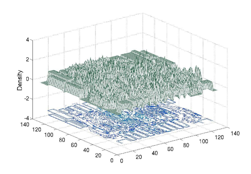
(a)

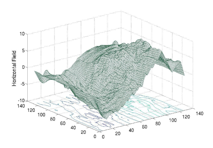
(b)

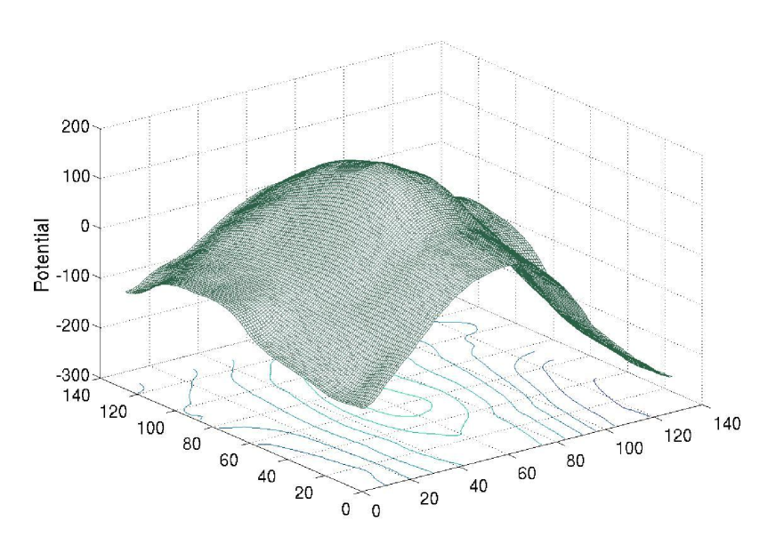
(c)

Figure 1: The distribution of electric (a) density (b) field (c) potential without filler insertion. Snapshots are extracted at iteration 50 of ADAPTEC1.

III-A Electrostatic Equilibrium

We use electric force for cell movement direction and density equalization. Direct-current (DC) component is removed from the density function such that under-filled regions become negatively charged. Cells locating at positive regions are attracted for neutralization. In the end, the system reaches the electrostatic equilibrium state with zero bin density and potential energy.

III-B Potential Energy Computation

Similar to [2, 4], we add disconnected ”fillers” to induce density force for connected cells clotting thus interconnect shortenning. Placement region could be irregular polygon (bounding box $R$). We name each non-placeable rectangular region within $R$ as a “dark node”. Cells are pushed away by the density force when approaching the chip boundary. Also, the area of fixed and dark nodes must be scaled down by the target density to globally balance the density force. Let $V_{fc}$ and $V_{d}$ denote the sets of fillers and dark nodes and $V^{\prime}=V_{m}\cup V_{f}\cup V_{fc}\cup V_{d}$, the potential energy is computed as

$$N(\vec{v})=\sum_{i\in V^{\prime}}N_{i}=\sum_{i\in V^{\prime}}q_{i}\psi_{i}.$$ (6)

III-C Density Constraint Formulation

By applying the penalty factor $\lambda$, we formulate an unconstrained optimization problem

$$\min_{\vec{v}}f(\vec{v})=\widetilde{W}(\vec{v})+\lambda N(\vec{v}).$$ (7)

Compared to the quadratic penalty method [5, 8] or the multiple constraints [4], our method has lower complexity and better quality. The gradient vector is $\nabla f=\nabla W+\vec{q}\cdot\vec{E}$ where $\vec{q}$ and $\vec{E}$ are the electric quantity and field vectors of all the cells. As the electric force always points to the steepest descent of system energy, we could dynamically balance the wirelength and density forces using penalty factors.

III-D Well-Defined Poisson’s Equation

By Gauss’ law, the potential and field are coupled with density by Poisson’s equation.

$$\begin{cases}\nabla\cdot\nabla\psi(x,y)=-\rho(x,y)\text{,}\\ \mathbf{\hat{n}}\cdot\nabla\psi(x,y)=\mathbf{0}\text{, }(x,y)\in\partial R,\\ \iint\limits_{R}\psi(x,y)=0\text{.}\\ \end{cases}$$ (8)

$\hat{n}$ is the outer unit normal and $\partial R$ is the boundary of $R$. $\nabla\cdot\nabla\equiv\frac{\partial^{2}}{\partial x^{2}}+\frac{\partial^{2}}{\partial y^{2}}$ is a differential operator. As electric force decreases to zero at boundary to prevent cells from moving outside, we select Neumann boundary condition. The potential integral is set to zero thus Poisson’s equation has unique solution.

III-E Fast Numerical Solution

We use fast Fourier transform to solve the Poisson’s equation [17]. Discrete sine transform (DST) is used to represent the electric field, which well satisfies the Neumann boundary condition. Therefore, potential and density functions are represented by discrete cosine transform (DCT). We first mirror the function domain from $[0,n-1]\times[0,n-1]$ to $[-n,n-1]\times[-n,n-1]$, then periodically extend it to infinity. The density function can thus be expressed as

$$\rho(x,y)=\sum_{u}\sum_{v}a_{u,v}\cos(w_{u}x)\cos(w_{v}y)\text{,}\\$$ (9)

where $w_{u}=\pi\frac{u}{n}$ and $w_{v}=\pi\frac{v}{n}$ are frequency components and $a_{u,v}$ are coefficients.

$$a_{u,v}=\frac{1}{2n}\sum_{x}\sum_{y}\rho(x,y)\cos(w_{u}x)\cos(w_{v}y)\text{.}\\$$ (10)

The solution to the potential function can be expressed as

$$\psi(x,y)= \sum_{u}\sum_{v}\frac{a_{u,v}}{w_{u}^{2}+w_{v}^{2}}\cos(w_{u}x)\cos(w_{v}y).$$ (11)

Therefore, we have the electric field distribution $E(x,y)=(E_{x},E_{y})$ shown as below

$$\begin{cases}E_{x}(x,y)=\sum_{u}\sum_{v}\frac{a_{u,v}w_{u}}{w_{u}^{2}+w_{v}^{2}}\sin(w_{u}x)\cos(w_{v}y),\\ E_{y}(x,y)=\sum_{u}\sum_{v}\frac{a_{u,v}w_{v}}{w_{u}^{2}+w_{v}^{2}}\cos(w_{u}x)\sin(w_{v}y).\\ \end{cases}$$ (12)

The above equations can be efficiently solved using many FFT algorithms [1]. Suppose we have $m$ cells in the netlist. In each iteration, we reset the grid density using $O(n^{2})$ time followed by density update using $O(m)$ time due to netlist traversal. The FFT computation consumes $O(n^{2}\log n^{2})$ time. In Section IV-A we define $n=O(\sqrt{m})$ thus the total complexity is essentially $O(m\log m)$.

IV Global Placement Algorithm

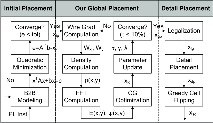
Figure 2: The entire flow of initial, global and detail placement.

The flow of the entire placement optimization is shown in Figure 2. The initial placement solution $\vec{x}_{ip}$ is based on quadratic wirelength minimization using bound-2-bound (B2B) net model [18]. The global placement problem is solved using nonlinear Conjugate Gradient (CG) method. After global placement completes, all the filler cells are removed from the solution $\vec{x}_{gp}$, which is then legalized and discretely optimized using FastDP [14]. with greedy flipping [3].

IV-A Self-Adaptive Parameter Adjustment

Grid dimension $n$ is statically determined before the global placement based on the number of cells $m=|A_{m}|$. As required to be power of 2 in [1], we set $n=\lceil\log_{2}\sqrt{m}\rceil$ with upper-bound of $1024$. Step length correlates with the search interval of which the length is dynamically updated. The initial value is determined as $\alpha^{max}_{0}=0.044w_{b}$, where $w_{b}$ is the grid width. The search interval is iteratively updated as $\alpha^{max}_{k}=\max(\alpha^{max}_{0},2\alpha_{k})$ and $\alpha^{min}_{k}=0.01\alpha^{max}_{k}$. Penalty factor is initially set as [5, 8]. Unlike those methods with constant scaling, we iteratively update $\lambda_{k}=\mu_{k}\lambda_{k-1}$ to balance the wirelength and density forces. The scaling factor is determined by $\mu_{k}=1.1^{-\frac{\Delta w_{k}}{\Delta w_{ref}}+1.0}$ based on HPWL variation $\Delta w_{k}=W(\vec{v}_{k})-W(\vec{v}_{k-1})$. In practice, we set the reference variation $\Delta w_{ref}=3.5\times 10^{5}$ and bound $\mu_{k}$ by $[0.75,1.1]$. Density overflow is used to terminate the global placement process Similar to Eq. (11) in [5], we use the density overflow $\tau$ as the stopping criterion The global placer terminates when $\tau\leq 10\%$. As illustrated in Figure 3(a), system energy is consistent with the density overflow.

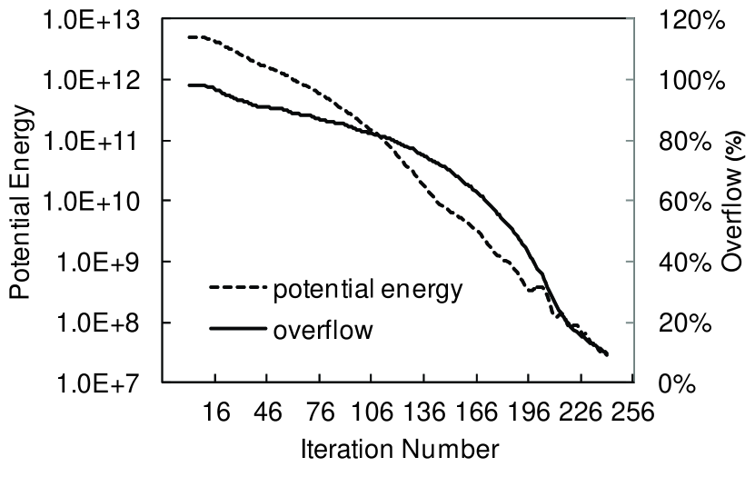
(a)

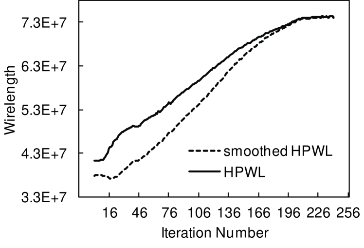
(b)

Figure 3: The illustration of (a) total overflow ratio $\tau$ and potential energy $N$ (b) total HPWL $W$ and smoothed wirelength $\widetilde{W}$.

Wirelength coefficient is used together with WA model [6] to smooth the HPWL as Figure 3(b) shows. The smoothing parameter $\gamma$ is larger at early time to encourage global movement and smaller at later iterations to enable movement of only HPWL-insensitive cells. We set the smoothing parameter as $\gamma=8.0w_{b}\times 10^{20/9\times\left(\tau-0.1\right)-1.0}$.

IV-B Global Placement

The detail flow of our global placement method FFTPL is shown in Algorithm 1. We solve the Poisson’s equation at line 5 by FFT library call [1]. The global placement solution $x_{gp}$ is output to the legalizer and detail placer at line 13.

Algorithm 1 FFTPL

0:  initial placement solution $\vec{x}_{0}=\vec{x}_{ip}$

0:  global placement solution $\vec{x}_{gp}$

1:  initialize $\lambda_{0}$, $\alpha^{max}_{0}$.

2:  for $k=1\to 1000$ do

3:     $f_{k-1}=f(\vec{x}_{k-1})=\widetilde{W}(\vec{x}_{k-1})+\lambda_{k-1}N(\vec{x}_{k-1})$

4:     compute density function $\rho_{k-1}$

5:     $(\psi_{k-1},\vec{E}_{k-1})=$FFTsolver$(\rho_{k-1})$

6:     compute gradient $\nabla f_{k-1}=\nabla\widetilde{W}_{k-1}+\lambda_{k-1}\nabla N_{k-1}$

7:     $\vec{x}_{k}=$CGsolver$\left(\vec{x}_{k-1},f_{k-1},\nabla f_{k-1},\alpha^{max}_{k-1},0.01\alpha^{max}_{k-1}\right)$

8:     update $\alpha_{k}^{max}$, $\lambda_{k}$, $\tau_{k}$, $\gamma_{k}$

9:     if $\tau_{k}\leq 10\%$ then

10:        $\vec{x}_{gp}=\vec{x}_{k}$, break

11:     end if

12:  end for

13:  return $\vec{x}_{gp}$

V Experiments and Results

TABLE I: HPWL ($\times 10^{6}$) and runtime (minutes) of all the placers on the ISPD 2005 benchmark suite [12] using official script for performance evaluation. Experiments are conducted under our 2.67GHz linux machine in single-thread mode. Average results are normalized to that of FFTPL (our work).

Categories		Min-Cut		Quadratic		Nonlinear
Placers		Capo10.5 [3]		FastPlace3.0 [20]		APlace2 [8]		NTUPlace3 [5]		mPL6 [4]		FFTPL
Circuits [12]	#Cells	HPWL	CPU	HPWL	CPU	HPWL	CPU	HPWL	CPU	HPWL	CPU	HPWL	CPU
ADAPTEC1	211K	87.80	48.33	78.34	2.92	78.35	48.88	80.29	7.17	77.93	23.27	76.46	9.17
ADAPTEC2	255K	102.66	61.63	93.47	4.13	95.70	68.07	90.18	8.22	92.04	24.75	85.57	12.67
ADAPTEC3	452K	234.27	133.43	213.48	9.53	218.52	186.67	233.77	18.53	214.16	73.97	202.16	45.40
ADAPTEC4	496K	204.33	141.85	196.88	8.75	209.28	209.60	215.02	23.53	193.89	71.03	185.83	34.33
BIGBLUE1	278K	106.58	77.90	96.23	4.57	100.02	64.05	98.65	14.30	96.80	30.05	91.64	23.63
BIGBLUE2	558K	161.68	150.15	154.89	8.00	153.75	136.43	158.27	35.10	152.34	79.00	145.54	30.83
BIGBLUE3	1097K	403.36	373.87	369.19	21.05	411.59	289.78	346.33	38.77	344.10	104.63	359.00	116.67
BIGBLUE4	2177K	871.29	730.42	834.04	40.13	945.77	779.22	829.09	106.08	829.44	238.82	805.90	165.00
Average		1.14$\times$	4.13$\times$	1.05$\times$	0.25$\times$	1.10$\times$	4.41$\times$	1.07$\times$	0.66$\times$	1.04$\times$	1.80$\times$	1.00$\times$	1.00$\times$

We implement our algorithm using C programming language and execute the program in a Linux operating system with Intel i7 920 2.67GHz CPU and 12GB memory. In our experiments, we use the benchmark suite from [12]. The target placement density $\rho_{t}$ is set to be $1.0$ for all the benchmarks. There is no parameter tuning towards specific benchmarks.

We include five cutting-edge placers for performance comparison with their source code or binary obtained. All the results are shown in Table I. On average, our placer improves the total wirelength by $13.58\%$, $5.14\%$, $10.24\%$, $7.20\%$ and $3.62\%$ over Capo10.5 [3], FastPlace3.0 [20], APlace2 [8], NTUPlace3 [5] and mPL6 [4], respectively. Compared to the published results in RQL [19] and SimPL [9], our placer produces better solutions in six and seven out of the totally eight benchmarks, respectively.

VI Conclusion

In this paper, we propose a flat nonlinear global placement algorithm with improved quality and efficiency. The placement instance is modeled as an electrostatic system, where electric potential and field are computed using Poisson’s equation. In future, we will extend our algorithm to parallel platform and other design objectives (timing, congestion, etc.).

VII Acknowledgement

The authors would like to acknowledge the support of NSF CCF-1017864.

References

- [1] General Purpose FFT Package, http://www.kurims.kyoto-u.ac.jp/~ooura/fft.html.
- [2] S. N. Adya, I. L. Markov, and P. G. Villarrubia. On Whitespace and Stability in Mixed-Size Placement. In ICCAD, pages 311–318, 2003.
- [3] A. E. Caldwell, A. B. Kahng, and I. L. Markov. Can Recursive Bisection Alone Produce Routable Placements? In DAC, pages 477–482, 2000.
- [4] T. F. Chan, J. Cong, J. R. Shinnerl, K. Sze, and M. Xie. mPL6: Enhanced Multilevel Mixed-Size Placement. In ISPD, pages 212–214, 2006.
- [5] T.-C. Chen, Z.-W. Jiang, T.-C. Hsu, H.-C. Chen, and Y.-W. Chang. NTUPlace3: An Analytical Placer for Large-Scale Mixed-Size Designs with Preplaced Blocks and Density Constraint. IEEE TCAD, 27(7):1228–1240, 2008.
- [6] M.-K. Hsu, Y.-W. Chang, and V. Balabanov. TSV-Aware Analytical Placement for 3D IC Designs. In DAC, pages 664–669, 2011.
- [7] A. B. Kahng, J. Lienig, I. L. Markov, and J. Hu. VLSI Physical Design: From Graph Partitioning to Timing Closure. Springer, 2010.
- [8] A. B. Kahng, S. Reda, and Q. Wang. Architecture and Details of a High Quality, Large-Scale Analytical Placer. In ICCAD, pages 890–897, 2005.
- [9] M.-C. Kim, D.-J. Lee, and I. L. Markov. SimPL: An Effective Placement Algorithm. In ICCAD, pages 649–656, 2010.
- [10] J. Lu, W.-K. Chow, C.-W. Sham, and E. F. Y. Young. A Dual-MST Approach for Clock Network Synthesis. In ASPDAC, pages 467–473, 2010.
- [11] J. Lu and C.-W. Sham. LMgr: A Low-Memory Global Router with Dynamic Topology Update and Bending-Aware Optimum Path Search. In ISQED, pages 231–238, 2013.
- [12] G.-J. Nam, C. J. Alpert, P. Villarrubia, B. Winter, and M. Yildiz. The ISPD2005 Placement Contest and Benchmark Suite. In ISPD, pages 216–220, 2005.
- [13] W. C. Naylor, R. Donelly, and L. Sha. Non-Linear Optimization System and Method for Wire Length and Delay Optimization for an Automatic Electric Circuit Placer. In US Patent 6301693, 2001.
- [14] M. Pan, N. Viswanathan, and C. Chu. An Efficient and Effective Detailed Placement Algorithm. In ICCAD, pages 48–55, 2005.
- [15] C. Sechen and A. Sangiovanni-Vincentelli. TimberWolf3.2: A New Standard Cell Placement and Global Routing Package. In DAC, pages 432–439, 1986.
- [16] C.-W. Sham, E. F. Y. Young, and J. Lu. Congestion Prediction in Early Stages of Physical Design. ACM TODAES, 12:1–12, 2009.
- [17] G. Skollermo. A Fourier Method for the Numerical Solution of Poisson’s Equation. Mathematics of Computation, 29(131):697–711, 1975.
- [18] P. Spindler, U. Schlichtmann, and F. M. Johannes. Kraftwerk2 - A Fast Force-Directed Quadratic Placement Approach Using an Accurate Net Model. IEEE TCAD, 27(8):1398–1411, 2008.
- [19] N. Viswanathan, G.-J. Nam, C. J. Alpert, P. Villarrubia, H. Ren, and C. Chu. RQL: Global Placement via Relaxed Quadratic Spreading and Linearization. In DAC, pages 453–458, 2007.
- [20] N. Viswanathan, M. Pan, and C. Chu. FastPlace3.0: A Fast Multilevel Quadratic Placement Algorithm with Placement Congestion Control. In ASPDAC, pages 135–140, 2007.