Measure synchronization in quantum many-body systems

Abstract

The concept of measure synchronization between two coupled quantum many-body systems is presented. In general terms we consider two quantum many-body systems whose dynamics gets coupled through the contact particle-particle interaction. This coupling is shown to produce measure synchronization, a generalization of synchrony to a large class of systems which takes place in absence of dissipation. We find that in quantum measure synchronization, the many-body quantum properties for the two subsystems, e.g., condensed fractions and particle fluctuations, behave in a coordinated way. To illustrate the concept we consider a simple case of two species of bosons occupying two distinct quantum states. Measure synchronization can be readily explored with state-of-the-art techniques in ultracold atomic gases and, if properly controlled, be employed to build targeted quantum correlations in a sympathetic way.

I Introduction

Since its discovery by Huygens when observing coupled pendula in the 17th century Pen , synchronization has been described in physics, chemistry, biology and even social behavior Review ; Review2 ; Review4 , becoming a paradigm for research of collective dynamics. It has been thoroughly studied in classical nonlinear dynamical systems Review3 , and extended to chaotic ones Chaos . Only recently synchronization has been studied in quantum systems, e.g., two coupled quantum harmonic oscillators Syn6 , a qubit coupled to a quantum dissipative driven oscillator Syn3 , two dissipative spins Syn4 , and two coupled cavities Syn5 . Last year, connections between quantum entanglement and synchronization have been discussed in continuous variable systems  Zam2 ; Syn7 .

A decade ago, Hampton and Zanette introduced a new concept termed measure synchronization (MS) for coupled Hamiltonian systems MS99 . They found that two coupled Hamiltonian systems experience a synchronization transition from a state in which the two subsystems visit different phase space regions to a state in which “their orbits cover the same region of the phase space with identical invariant measures” MS99 . The control parameter is the coupling strength between the two subsystems.

The key difference between MS and conventional synchronization is that MS takes place in absence of dissipation. In standard synchronization dissipation plays a key role, as it is responsible for the collapse of any trajectory of the system in phase space. For coupled Hamiltonian systems, phase space volume must be conserved following Liouville’s theorem, thus preventing the collapse of any trajectory in phase space. In the case of MS, two coupled Hamiltonian systems become synchronized when they cover the same phase space domain, without requiring that the synchronized systems have the same evolution trajectories.

In this article we introduce measure synchronization, a concept up to now only considered in a classical framework, into the quantum many-body regime. First exploratory studies of measure synchronization in quantum systems have been done in different contexts, i.e., MS has been discussed in coupled Hamiltonian systems associated with nonlinear Schrödinger equations MS05 ; also, MS transitions have been revealed on meanfield theories describing condensed bosonic quantum many-body systems MS03 ; Qiu10 ; MS12 ; Qiu13 . However, it is worth stressing that in the above cases the dynamical variables describing these quantum systems are classical, i.e. quantum fluctuations are neglected, a reasonable approximation in bosonic systems which are fully condensed Leggett01 . This made the correspondence between the classical MS concept introduced in Ref. MS99 and the MS studies of these quantum systems straightforward. So conceptually, measure synchronization discussed in these contexts remained classical. Here, we tackle the problem in a fully many-body quantum mechanical way. A major conceptual difference is that, in the general case we need to identify quantum many-body observables which allow us to characterize MS-like behaviors provided the very definition of the area covered by each subsystem in phase space is absent.

We consider two quantum many-body systems (QMBS) which are coupled through a local interaction term. Our main finding is that we characterize a crossover behavior from non-MS to MS in the evolution of the quantum many-body properties of the subsystems. This implies that two QMBS, which if non coupled would develop different quantum correlations, will, if sufficiently coupled, have similar condensed fractions, particle fluctuations, etc. This is an effect which will affect the behavior of future QMBS and quantum simulators, and which, if properly controlled, can be employed to share or to induce quantum correlations between different degrees of freedom in the system. MS is a dynamical feature which we will show to appear in the evolution of QMBS. It describes how, under certain premises, the dynamics of two weakly coupled quantum subsystems becomes coherent after a short transient time. MS describes how two subsets of a QMBS will evolve in a collective way, exchanging energy during the full evolution, exploring similar average values of relevant observables and developing similar quantum correlations.

It is worth emphasizing that our ability to understand and utterly control quantum correlations in QMBS is the key to producing powerful technological applications. A notable recent example is the case of pseudo-spin squeezed states WI94 , which can be produced in bosonic Josephson junctions esteve08 . In this case, producing fragmented ultracold gases is shown to notably raise the precision achievable in quantum metrology experiments gross10 ; riedel10 . These applications will become a reality in the near future thanks to the miniaturization of ultracold atomic systems nshii13 . As shown here, MS can be used to transfer, or sympathetically produce, fragmentation in one subsytem of the QMBS which can, for instance, improve interferometric signals.

The article is organized in the following way. In Sec. II we describe the many-body Hamiltonian. In Sec. III we present our results, concerning the onset of MS and how it shows in the many-body properties of the system. In Sec. IV we sketch an experimental implementation with ultracold atomic gases. A summary and conclusions are provided in Sec. V.

II Many-body hamiltonian

To illustrate the many-body quantum MS we consider the simplest implementation we can think of. These are two different kinds of bosons, $A$ and $B$, populating solely two quantum states, $L$ and $R$. We will consider a linear coupling between the two quantum states and contact interaction for $AA$, $AB$, and $BB$ bosons. The many-body Hamiltonian considered for $N_{A}$ and $N_{B}$ atoms in two modes is,

$$\hat{H} = \hat{H}_{A}+\hat{H}_{B}+\hat{H}_{AB},$$ (1)

where

$$\hat{H}_{A} = \frac{U_{A}}{2}\left[(\hat{a}_{L}^{{\dagger}}\hat{a}_{L})^{2}+(\hat{a}_{R}^{{\dagger}}\hat{a}_{R})^{2}\right]-J_{A}(\hat{a}_{L}^{{\dagger}}\hat{a}_{R}+\hat{a}_{R}^{{\dagger}}\hat{a}_{L})$$

$$\hat{H}_{B} = \frac{U_{B}}{2}\left[(\hat{b}_{L}^{{\dagger}}\hat{b}_{L})^{2}+(\hat{b}_{R}^{{\dagger}}\hat{b}_{R})^{2}\right]-J_{B}(\hat{b}_{L}^{{\dagger}}\hat{b}_{R}+\hat{b}_{R}^{{\dagger}}\hat{b}_{L})$$

$$\hat{H}_{AB} = U_{AB}(\hat{a}_{L}^{{\dagger}}\hat{a}_{L}\hat{b}_{L}^{{\dagger}}\hat{b}_{L}+\hat{a}_{R}^{{\dagger}}\hat{a}_{R}\hat{b}_{R}^{{\dagger}}\hat{b}_{R})\,.$$ (2)

$\hat{a}_{L(R)}^{{\dagger}}$ $(\hat{a}_{L(R)})$ and $\hat{b}_{L(R)}^{{\dagger}}$ $(\hat{b}_{L(R)})$ are creation (annihilation) operators for the single-particle modes $L$ or $R$ of the two species. The terms proportional to $J_{A(B)}$ are the linear coupling terms, which in absence of any interaction would induce periodic Rabi oscillations of the populations between the states $L$ and $R$. $U_{A}$, $U_{B}$, and $U_{AB}$ measure the $AA$, $BB$, and $AB$ contact interactions. The $U_{AB}$ term is the only one coupling the dynamics of the $A$ and $B$ subsystems, and will be responsible for the MS between both of them.

The Hamiltonian can be numerically diagonalized in the $N_{D}=(N_{A}+1)(N_{B}+1)$ dimensional space spanned by the many-body Fock basis tensor product of the $A$ and $B$ Fock states, e.g., for the $A$, $|N_{A,L}\rangle\equiv 1/\sqrt{N_{A,L}!N_{A,R}!}\ (\hat{a}^{\dagger}_{L})^{N_{A,L}}(\hat{a}^{\dagger}_{R})^{N_{A,R}}|{\rm vac}\rangle$, with $N_{A,L}=0,\dots,N_{A}$ and $N_{A,R}=N_{A}-N_{A,L}$. The most general $N$-particle state can be written as

$$|\Psi\rangle=\sum_{N_{A,L}=0}^{N_{A}}\sum_{N_{B,L}=0}^{N_{B}}c_{N_{A,L},N_{B,L}}\ |N_{A,L},N_{B,L}\rangle\,.$$ (3)

The time evolution of any given initial state is governed by the time dependent Schrödinger equation, $i\,\hbar\,\partial_{t}|\Psi(t)\rangle=\hat{H}|\Psi(t)\rangle$. Once we have computed the many-body state, we can obtain average particle numbers on modes $L$ and $R$, $\langle N_{A,\alpha}\rangle=\langle\Psi|\hat{a}^{\dagger}_{\alpha}\hat{a}_{\alpha}|\Psi\rangle$, $\langle N_{B,\alpha}\rangle=\langle\Psi|\hat{b}^{\dagger}_{\alpha}\hat{b}_{\alpha}|\Psi\rangle$, with $\alpha=L,R$. The imbalance of population for each species is defined as $Z_{A(B)}=(N_{A(B),L}-N_{A(B),R})/N_{A(B)}$.

To characterize the degree of condensation of each subsystem, $A$ and $B$, at any given time we will make use of the one-body density matrix, $\rho$ ours10 . For a state $|\Psi\rangle$ it is defined as, e.g., for species $A$, $\rho^{A}_{ij}=\langle\Psi|\hat{\rho}^{A}_{ij}|\Psi\rangle$, with $\hat{\rho}^{A}_{ij}=a^{\dagger}_{i}a_{j}$, and $i,j=L,R$. The traces of $\rho^{A}$ and $\rho^{B}$ are normalized to the number of atoms in each subsystem, $N_{A}$ and $N_{B}$. The two normalized eigenvalues (divided by the total number of atoms $N_{A}$) are $n_{a_{1}(a_{2})}$, with $n_{a_{1}}\geq n_{a_{2}}\geq 0$. We always have $n_{a_{1}}+n_{a_{2}}=1$. The larger eigenvalue is also called the condensed fraction. Similar definitions are used for species $B$.

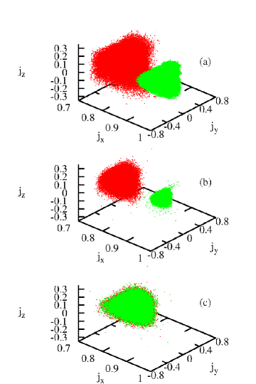
Figure 1: (Color online) Measure synchronization. Quantum many-body measure synchronization characterized by the domain covered during the evolution of each subsystem on the 3D space defined by the average value of the pseudo-angular momentum, $j_{x}\equiv(2/N)\langle\hat{J}_{x}\rangle$, $j_{y}\equiv(2/N)\langle\hat{J}_{y}\rangle$, and $j_{z}\equiv(2/N)\langle\hat{J}_{z}\rangle$ for species $A$ (red) and $B$ (green). (a) $U_{AB}=0$ (non-MS), (b) $U_{AB}=0.008\ U$ (non-MS), and (c) $U_{AB}=0.5\ U$ (MS). In panel (c) the two clouds overlap. $Z_{A}(0)=0.2$, $Z_{B}(0)=0.4$, and $N_{A}=N_{B}=30$. In all panels the points correspond to periodic moments within one time evolution, we show them as dots, instead of a continuous line, to avoid one of the species hiding the other one.

A way to characterize the transition from non-MS to MS dynamics in classical systems is by looking at the time average of the energies of subsystems $A$ and $B$ Qiu13 ; MS03 . In MS dynamics, both subsystems cover, with equal density, the same phase space domain, which reflects on equal long-time averages of the energies of the subsystems defined as

$$\bar{E}_{A(B)}={1\over T}\int_{0}^{T}\ E_{A(B)}(t)\ dt\ ,$$ (4)

where the expectation values of the energy for each subsystem $A$ (and $B$) at time $t$ are $E_{A}(t)=\langle\Psi(t)|\hat{H}_{A}|\Psi(t)\rangle$, and $E_{B}(t)=\langle\Psi(t)|\hat{H}_{B}|\Psi(t)\rangle$, with $|\Psi(t)\rangle$ the evolved quantum state.

III Results

We set both intraspecies interactions to be the same, i.e. , $U\equiv U_{A}=U_{B}$, with $NU/J=7.2$, and also choose equal linear couplings, $J\equiv J_{A}=J_{B}$. We take as a unit of time the Rabi time, $t_{\rm Rabi}=\pi/J$, and as a unit of energy, $\hbar/t_{\rm Rabi}$. Our initial states will in all cases be coherent states for both the $A$ and $B$ species, in which all atoms populate the single particle state $(1/\sqrt{2})(\cos\theta/2\ \hat{a}^{\dagger}_{L}+\sin\theta/2\ a^{\dagger}_{R})$ [with initial population imbalance, $Z(0)=\cos\theta$]. These states will evolve under the action of the many-body Hamiltonian. We will look for a transition from non-MS to MS in the collective dynamics of the many-body state as we vary the interspecies interaction strength $U_{AB}$.

The transition from non-MS to MS dynamics is shown in Fig. 1. We plot the average value of the pseudo-angular momentum operators which can readily be constructed from the creation and annihilation operators of each species Leggett01 , $\hat{J}_{x}=(1/2)(\hat{a}^{\dagger}_{L}\hat{a}_{R}+\hat{a}_{L}\hat{a}^{\dagger}_{R})$, $\hat{J}_{y}=1/(2i)(\hat{a}^{\dagger}_{L}\hat{a}_{R}-\hat{a}_{L}\hat{a}^{\dagger}_{R})$, $\hat{J}_{z}=(1/2)(\hat{a}^{\dagger}_{L}\hat{a}_{L}-\hat{a}^{\dagger}_{R}\hat{a}_{R})$. In our conditions, fixed $N_{A}$ and $N_{B}$, these operators build the symmetric representation of $SU(2)$ of dimension $N_{A}+1$ and $N_{B}+1$. As shown in the three-dimensional (3D) figure, in the non-MS cases, $U_{AB}=0$ and $U_{AB}=0.008\ U$, the domains of ($\langle J_{x}\rangle$, $\langle J_{y}\rangle$, $\langle J_{z}\rangle$) explored by each subsystem are disjointed. In the MS case, however, both domains completely overlap. This feature can be regarded as the many-body counterpart of the classical definition of MS, in which the phase space domain covered by both subsystems is the same.

In classical systems MS implies that both subsystems have similar long-time averages of their energies. Importantly, the non-MS to MS transition in classical systems is discontinuous, which allows one to define a critical point to characterize the dynamical phase transition MS99 . This is seen in Fig. 2, where we depict the average energy $\langle E_{A}\rangle$ and $\langle E_{B}\rangle$ as a function of the interspecies interaction $U_{AB}$, with $\bar{E}_{A}=\bar{E}_{B}$ characterizing MS. The classical results Qiu13 , depicted in green and blue, feature the known discontinuity. In the many-body case the situation is different; the dynamical phase transition is replaced by a crossover behavior, therefore no critical point can be unambiguously defined. There is no criticality which involves logarithmic singularity in the quantum measure synchronization as compared with classical theory of measure synchronization MS03 ; Qiu13 . Also note that in the many-body case, MS appears at higher values of $U_{AB}$ as compared to the classical transition. The inset in Fig. 2 shows the behavior of $E_{A}(t)$ and $E_{B}(t)$ for the two different regions. In the MS case, the two subsystems exchange energy in such a way that their energies oscillate around the same average value maintaining an almost constant sum. In the non-MS dynamics, the energies of the subsystems are never fully exchanged, and $A$ has always more average energy than $B$. For different initial conditions, particle numbers, and parameters $NU/J$ we obtain a similar picture (see Appendix A), the main difference being the size of the MS and non-MS regions.

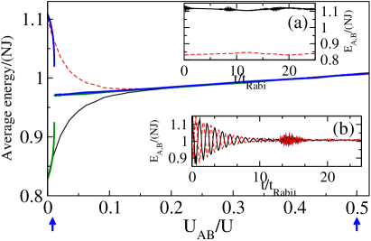
Figure 2: (Color online) From non-MS to MS. Long-time averaged energies, Eq. (4), for the two species $\bar{E}_{A}$ (solid) and $\bar{E}_{B}$ (dashed) as a function of $U_{AB}$. MS dynamics corresponds to equal averages, $\bar{E}_{A}=\bar{E}_{B}$. $Z_{A}(0)=0.2$, $Z_{B}(0)=0.4$, and $N_{A}=N_{B}=30$. In the insets we depict $E_{A}(t)$ and $E_{B}(t)$ for two specific values of $U_{AB}/U=0.008$ (a) and $U_{AB}/U=0.5$ (b). The two values are marked with arrows in the main figure. $T=1000\ t_{\rm Rabi}$. The green and blue lines correspond to the classical prediction of Ref. Qiu13 .

Now we concentrate on the evolution of the many-body properties of both subsystems. In Fig. 3 we consider the same initial state and two values of $U_{AB}$, $0.008\ U$ and $0.5\ U$, giving rise to non-MS and MS, respectively. Figure 3, panels (a) and (b) show the population imbalance between the two quantum states ($L$ and $R$) for each subsystem. The quantum many-body evolution becomes apparent, with characteristic collapse and revival dynamics ima97 . This collapse and revival dynamics has been addressed for single component junctions Milburn97 ; JAME06 and it can be understood in finite systems due to the finite number of frequencies entering in any dynamical evolution in the system.

We note that before reaching MS, the dynamics of the two subsystems is different both in the amplitude of the oscillation and on the times for collapses and revivals. After reaching MS, the times for collapses and revivals are the same. This striking feature provides a way to characterize quantum measure synchronization in the rhythms of the coupled Hamiltonian systems. Furthermore, we note that the oscillating amplitude for the two subsystems will be the same once MS is achieved, which is a feature that also shows in classical measure synchronization states MS12 .

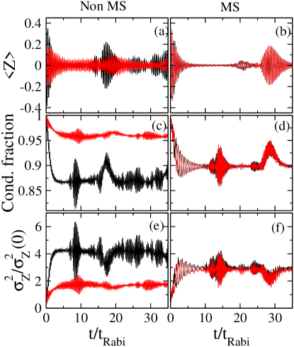
Figure 3: (Color online) Measure synchronization on the many-body properties. We compare the properties of both subsystems $A$ (black) and $B$ (red) as a function of time, for a non-MS dynamics, $U_{AB}=0.008\ U$ (left panels) and for MS dynamics, $U_{AB}=0.5\ U$ (right panels). The population imbalances [(a), (b)], condensed fractions [(c), (d)], and dispersion of the population imbalance $\sigma^{2}_{Z}=\langle Z^{2}\rangle-\langle Z\rangle^{2}$ [(e), (f)]. All magnitudes show a signature of the difference between the non-MS and MS dynamics. $Z_{A}(0)=0.2$, $Z_{B}(0)=0.4$, and $N_{A}=N_{B}=30$.

A crucial feature of quantum many-body bosonic systems is the appearance of correlations stronger than those present in Bose-Einstein condensed clouds. An initially condensed system loses condensation during the evolution, and becomes fragmented baym [see panels (c) and (d). This fragmentation also takes place if there is no coupling between the subsystems ours10 . Interestingly, in the MS dynamics, the condensed fraction of both subsystems gets clearly correlated after a very short transient time, having the same envelope of the oscillation amplitudes, which is a key feature of MS. This feature is found with all particle numbers studied $N_{A}=N_{B}\leq 80$ (see Appendix A). This similar behavior is also exhibited in the dispersions of particle differences [Fig. 3, panels (e) and (f)]. This is of special significance, as this is directly related to the emergence of cat-like many-body states or pseudo-spin squeezed states in the evolution ours10 . The latter provide a direct application of this physics to improve our precision measurements esteve08 .

IV Proposal for an experimental implementation

The aforementioned MS can be studied with state-of-the-art experimental techniques in ultracold atomic physics. The almost perfect decoupling of ultracold atoms from their environment enables the investigation of the quantum measure synchronization in conservative systems. We describe a feasible system which can simulate with good precision the many-body Hamiltonian in Eq. (1) using trapped ultracold atomic gases bloch-rmp ; lewenstein-book . We consider a two-species ultracold atomic cloud trapped in a symmetric double-well potential. In the weakly interacting regime, assuming the atom-atom interactions are correctly described by a contact interaction, and following similar steps as in Ref. Milburn97 , one obtains Eq. (1). The classical predictions of Eq. (1) have been studied in Refs. Ashhab02 ; diaz09 ; satija09 ; mazzarella10 ; naddeo10 ; mmm11 and some many-body features in Ref. weiss . The linear couplings $J$ are proportional to the energy splitting between the quasidegenerate ground state of the double-well potential. The atom-atom interaction terms, are given by $U_{\sigma}=(4\pi\hbar^{2}a_{\sigma}/m_{\sigma})\int{\left|{\varphi_{\sigma}}\right|}^{4}d{\bf r}$, $U_{AB}=2\pi\hbar^{2}a_{AB}(\frac{1}{{m_{A}}}+\frac{1}{{m_{B}}})\int{\left|{\varphi_{A}}\right|}^{2}\left|{\varphi_{B}}\right|^{2}d{\bf r}$, where $\sigma$ refers to atoms $A$ or $B$. $\varphi$ are localized single particle states; the localized single particle states have been normalized as $\int d{\bf r}|\varphi({\bf r})|^{2}=1$. $a_{\sigma}$ is $s$-wave scattering length between atoms $\sigma$, with mass $m_{\sigma}$. $a_{AB}$ is the interspecies $s$-wave scattering length. The scattering lengths are varied routinely in ultracold atom experiments by means of Feshbach resonances Fesh or confinement induced resonances conf . A possible specific experimental implementation could be an external double-well potential as in Ref. Albiez05 or the double-well inside the quantum chip used in Ref. berrada13 . It has been shown that two mode BECs can be prepared in coherent states experimentally Zibold10 ; luc11 . It would be possible to characterize quantum MS by investigating the times of collapses and revivals for the two species. There are also other experimental options for consideration, i.e., microcavity exciton-polaritons system car13 , or coupled micropillars system gal13 . Even though ultracold atomic samples are well isolated from the environment, there is one source of decoherence which could affect the onset of MS to non-MS transitions. This is the presence of losses in the system. These have been studied in detail for single component Josephson junctions, finding a constraint on the maximum attainable correlation which can be produced in the junction li08 . A study of the effect of losses on the MS to non-MS transition falls beyond the scope of the present article.

V Summary and conclusions

We introduced the concept of measure synchronization in quantum many-body systems. To exemplify the phenomenon we have considered a two-species bosonic Josephson junction made of a small number of atoms which can be experimentally studied in a number of different setups. Importantly, the measure synchronization occurs at the many-body quantum level, showing how properties such as the condensed fraction or the fluctuations in particle number of the two species behave coordinately above a certain coupling strength between the two systems. The findings reported apply to a variety of quantum many-body systems. An important application which can be envisaged is to profit from the MS described here to build targeted quantum correlations of certain degrees of freedom in the system in a sympathetic way. That is, when one can experimentally control and prepare the quantum correlations in one part of the system (e.g. one of the species), this method can be used to build similar quantum correlations in other parts of the system which cannot be experimentally controlled (e.g. the other species). In this MS regime, different parts of the system will develop similar quantum correlations and other quantum properties after a short transient time.

Appendix A Classical and full quantum descriptions

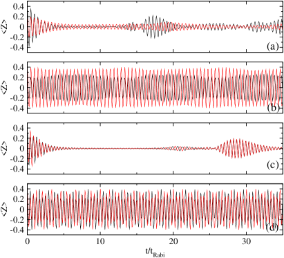
Figure 4: (Color online) Evolution of the population imbalance of both species. Comparison between the full quantum results shown in Fig. 3 and the classical predictions of Ref. Qiu13 . (a) and (b) are for the full quantum and classical prediction for a non-MS case ($U_{AB}=0.008U$), respectively. (c) and (d) are the full quantum and classical prediction for the MS case ($U_{AB}=0.5U$), respectively.

In this Appendix we analyze, by considering increasingly larger particle numbers, the relation between the classical and full quantum descriptions. The main interest of the present article is to extend the concept of measure synchronization to systems which do not accept a full classical description. Thus, we have emphasized the effects on the magnitudes which have no direct classical analog, such as the condensed fractions and the fluctuations of the particle numbers, shown in Figs. 3(c) and  3(d) and Figs.  3(e) and  3(f), respectively. Interestingly, particle number fluctuations can be measured experimentally and provide a good way of pinning down correlated states in these systems esteve08 ; Zibold10 .

To take the classical limit in a meaningful way we will perform exact numerical simulations for $N_{A}=N_{B}\leq 80$, keeping both $J$ and $NU/J=7.2$ constant, and compare to the corresponding classical predictions. As occurred in the case of a usual bosonic Josephson junction, the most remarkable difference between the classical and quantal results is the presence of quantum collapses and revivals in the latter Milburn97 . This can be seen already on the evolution of the average values of the particle number imbalances of species A and B. In Fig. 4 we depict the comparison between the average particle imbalance of each species reported in Fig. 3 (obtained for $N=30$) and the corresponding classical prediction Qiu13 . Also, this is one of the signatures that shows that MS can be characterized by the rhythms observed in the dynamical evolution of the two coupled subsystems. In contrast, classical measure synchronization is characterized by a spatial localization in the phase space associated to the conjugate variables describing the imbalance and the phase difference of each subsystem with no need of synchronization in the time evolution of the variables of each subsystem Qiu10 .

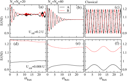
Figure 5: (Color online) Evolution of the energy of each subsystem. The upper and lower rows correspond to a MS and a non-MS situation, respectively. The value of $U_{AB}=0.008$ U for non-MS, and $U_{AB}=0.2$ U for the MS case. Exact many-body results for $N_{A}=N_{B}=20$ and $N_{A}=N_{B}=80$ are given panels [(a), (d)] and [(b), (e)], respectively. Panels [(c), (f)] contain the classical predictions Qiu13 . $Z_{A}(0)=0.2$ and $Z_{B}(0)=0.4$.

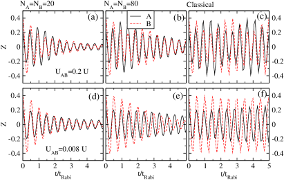
Figure 6: (Color online) Evolution of the population imbalance for both species. The upper and lower rows correspond to a MS and a non-MS situation, respectively. The value of $U_{AB}=0.008$ U for non-MS, and $U_{AB}=0.2$ U for the MS case. Exact many-body results for $N_{A}=N_{B}=20$ and $N_{A}=N_{B}=80$ are given panels [(a), (d)] and [(b), (e)], respectively. Panels [(c), (f)] contain the classical predictions Qiu13 . $Z_{A}(0)=0.2$ and $Z_{B}(0)=0.4$.

As expected, increasing the number of particles, the classical predictions better describe the initial behavior of the quantum ones. In Fig. 5 we present the average values of the energy of each subsystem as a function of time comparing the classical results to quantum ones at $N_{A}=N_{B}=20$ and 80. In the MS case $(U_{AB}=0.2U)$, panels (a)–(c), the classical result shows quasiperiodic oscillations for both $E_{A}(t)$ and $E_{B}(t)$. As expected for the MS case, both subsystems have the same mean energy, when averaged over long times. This feature is also present in the quantum calculation, as shown in Fig. 2 for $N_{A}=N_{B}=30$, already for $N_{A}=N_{B}=20$, Fig. 5 (a). In this case the oscillation is clearly damped for times around $5t_{\rm Rabi}$, departing from the classical results fairly early. As the total number of particles is increased to $N_{A}=N_{B}=80$, the time of the first collapse increases $\simeq 10t_{\rm Rabi}$. In Fig. 6 we depict the evolution of the average population imbalance in both situations, which clearly shows how the classical result improves the description of the initial time evolution as $N$ is increased.

In the non-MS situation the classical result departs earlier from the quantal predictions [see Fig. 5(d)–5(f)]. In this case, the classical case clearly shows different long-time-averaged values of the energies for each subsystem, a feature of non-MS. In the quantum results this is also observed, albeit in this case even for $N_{A}=N_{B}=80$ the classical and quantum results differ quantitatively already for times of the order of $3t_{\rm Rabi}$. Note the collapses and revivals inherent to the quantum description make it difficult to talk about long time averages of the signals.

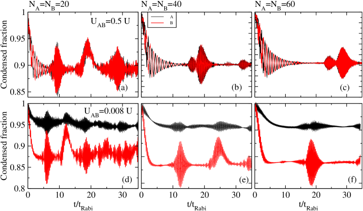
Figure 7: (Color online) The upper and lower rows correspond to a MS and a non-MS situation, respectively. The value of $U_{AB}=0.008U$ is for non-MS, and $U_{AB}=0.5U$ is for the MS case. Exact many-body results for $N_{A}=N_{B}=20$, 40 and 60, are given in panels [(a),(d)], [(b),(e)] and [(c),(f)], respectively. $Z_{A}(0)=0.2$ and $Z_{B}(0)=0.4$.

As discussed above, we find a synchronization of the fragmentation of the subsystems in the MS case as opposed to the non-MS situations. In the classical description this is of course absent, as the subsystems are fully condensed during the evolution. In the quantum case even for small number of particles $N_{A}=N_{B}=20$ we find this clear feature [see Fig. 7(a) and Fig. 7(d)]. In the MS case both subsystems clearly fragment in a synchronized way [Figs. 7(a) - 7(c)] as opposed to the non-MS case [Figs. 7(d)–7(f)]. Note also that MS produces more overall fragmentation in the system, as it is the less fragmented component A, the one that follows the more fragmented one B. The time scale in which the system fragments is found to be mostly independent of the number of particles, for the particle numbers considered. At $t\simeq 10t_{\rm Rabi}$ the maximum degree of correlation is already built in the system. Also the amount of fragmentation is found to be almost independent of the particle number considered, although as expected it decreases slowly with particle number.

References

- (1) C. Huygens, Horologium Oscillatorium (Apub F. Muquet, Parisiis, 1673).
- (2) Y. Kuramoto, Chemical Oscillations, Waves and Turbulence (Springer, Berlin) (1984).
- (3) Z. Néda, E. Ravasz, Y. Brechet, T. Vicsek, and A.-L. Barabási, Nature (London), 403, 850 (2000).
- (4) A. Arenas, A. Díaz-Guilera, J Kurths, Y. Moreno, and C. Zhou, Phys. Rep. 469 (3), 93 (2008).
- (5) A. Pikovsky, H. Rosenblum and J. Kurths, Synchronization. A Universal Concept in Nonlinear Sciences (Cambridge University Press, Cambridge, England, 2001).
- (6) L. M. Pecora and T. L. Carroll, Phys. Rev. Lett. 64, 821 (1990).
- (7) G. L. Giorgi, F. Galve, G. Manzano, P. Colet, and R. Zambrini, Phys. Rev. A 85, 052101 (2012).
- (8) O. V. Zhirov and D. L. Shepelyansky, Phys. Rev. B 80, 014519 (2009).
- (9) P. P. Orth, D. Roosen, W. Hofstetter, and K. LeHur, Phys. Rev. B 82, 144423 (2010).
- (10) T. E. Lee and M. C. Cross, Phys. Rev. A 88, 013834 (2013).
- (11) G. Manzano, F. Galve, G. L. Giorgi, E. Hernández-García, and R. Zambrini, Sci. Rep. 3, 1439 (2013).
- (12) A. Mari, A. Farace, N. Didier, V. Giovannetti, and R. Fazio, Phys. Rev. Lett. 111, 103605 (2013).
- (13) A. Hampton and D. H. Zanette, Phys. Rev. Lett. 83, 2179 (1999).
- (14) U. E. Vincent, A. N. Njan, and O. Akinlade, Mod. Phys. Lett. B 19, 737 (2005).
- (15) X. Wang, M. Zhan, C-H. Lai and H. Gang, Phys. Rev. E. 67, 066215 (2003).
- (16) H. B. Qiu, J. Tian and L-B Fu, Phys. Rev. A 81, 043613 (2010).
- (17) J. R. Zhang, H. Jiang, Y. Yang, W. S. Duan and J. M. Chen, Phys. Scr. 86, 065602 (2012).
- (18) J. Tian, H. B. Qiu, G. F. Wang, Y. Chen and L-B Fu, Phys. Rev. E 88, 032906 (2013).
- (19) A. J. Leggett, Rev. Mod. Phys. 73, 307 (2001).
- (20) D. J. Wineland, J. J. Bollinger, W. M. Itano, and D. J. Heinzen, Phys. Rev. A 50, 67 (1994).
- (21) J. Esteve, C. Gross, A. Weller, S. Giovanazzi, and M. K. Oberthaler, Nature (London) 455, 1216, (2008).
- (22) C. Gross, T. Zibold, E. Nicklas, J. Estève, and M. K. Oberhtaler, Nature (London) 464, 1165 (2010).
- (23) M. F. Riedel, P. Böhi, Y. Li, T. W. Hänsch, A. Sinatra, and P. Treutlein, Nature (London) 464, 1170 (2010).
- (24) C. C. Nshii, M. Vangeleyn, J. P. Cotter, P. F. Griffin, E. A. Hinds, C. N. Ironside, P. See, A. G. Sinclari, E. Riss, and A. S. Arnold, Nat. Nanotechnol. 8, 321 (2013).
- (25) B. Julia-Diaz, D. Dagnino, M. Lewenstein, J. Martorell, A. Polls, Phys. Rev. A 81, 023615 (2010).
- (26) A. Imamogglu, M. Lewenstein and L. You, Phys. Rev. Lett. 78, 2511 (1997).
- (27) G.J. Milburn, J. Corney, E. M. Wright, and D. F. Walls, Phys. Rev. A 55, 4318 (1997).
- (28) M. Jääskeläinen, and P. Meystre, Phys. Rev. A 71, 043603 (2005).
- (29) E. J. Mueller, T-L. Ho, M. Ueda, and G. Baym, Phys. Rev. A 74, 033612 (2006).
- (30) I. Bloch,, J. Dalibard, and W. Zwerger, Rev. Mod. Phys. 80, 885 (2008).
- (31) M. Lewenstein, A. Sanpera, V. Ahufinger, Ultracold Atoms in Optical Lattices: Simulating Quantum Many-Body Systems (Oxford University Press, 2013).
- (32) S. Ashhab and C. Lobo, Phys. Rev. A 66, 013609 (2002).
- (33) B. Juliá-Díaz, M. Guilleumas, M. Lewenstein, A. Polls, A. Sanpera, Phys. Rev. A 80, 023616 (2009).
- (34) I. I. Satija, R. Balakrishnan, P. Naudus, J. Heward, M. Edwards, C. W. Clark, Phys. Rev. A 79, 033616 (2009).
- (35) G. Mazzarella, M. Moratti, L. Salasnich, F. Toigo, J. Phys. B: At., Mol. Opt. Phys. 43, 065303 (2010).
- (36) A Naddeo, R Citro, J. Phys. B: At. Mol. Opt. Phys 43, 135302 (2010).
- (37) M. Mele-Messeguer, B. Julia-Diaz, M. Guilleumas, A. Polls, A. Sanpera, New J. Phys. 13, 033012 (2011).
- (38) N Teichmann, C Weiss, EPL 78, 10009 (2007).
- (39) S. B. Papp and C. E. Wieman, Phys. Rev. Lett. 97, 180404 (2006); S. B. Papp, J. M. Pino, and C. E. Wieman, Phys. Rev. Lett. 101, 040402 (2008); G. Thalhammer, G. Barontini, L. De Sarlo, J. Catani, F. Minardi, and M. Inguscio, Phys. Rev. Lett. 100, 210402 (2008); D. J. McCarron, H. W. Cho, D. L. Jenkin, M. P. Köppinger, and S. L. Cornish, Phys. Rev. A 84, 011603(R) (2011).
- (40) M. Olshanii, Phys. Rev. Lett. 81, 938 (1998).
- (41) M. Albiez, R. Gati, J. Fölling, S. Hunsmann , M. Cristiani and M. K. Oberthaler, Phys. Rev. Lett. 95, 010402 (2005).
- (42) T. Berrada, S. van Frank, R. Bücker, T. Schumm, J.-F. Schaff, J Schmiedmayer, Nat. Commun. 4, 2077 (2013).
- (43) T. Zibold, E. Nicklas, C. Gross, and M. K. Oberthaler, Phys. Rev. Lett. 105, 204101 (2010).
- (44) B. Lücke, M. Scherer, J. Kruse, L. Pezze, F. Deuretzbacher, P. Hyllus, O. Topic, J. Peise, W. Ertmer, J. Arlt, L. Santos, A. Smerzi, and C. Klempt, Science 334, 773 (2011).
- (45) I. Carusotto and C. Ciuti, Rev. Mod. Phys. 85 299 (2013).
- (46) M. Abbarchi, A. Amo, V. G. Sala, D. D. Solnyshkov, H. Flayac, L. Ferrier, I. Sagnes, E. Galopin, A. Lemaitre, G. Malpuech, and J. Bloch, Nat. Phys. 9, 275 (2013).
- (47) Y. Li, Y. Castin, A. Sinatra, Phys. Rev. Lett. 100, 210401 (2008).