Sampling-based Learning Control for Quantum Systems with Hamiltonian Uncertainties

Abstract

Robust control design for quantum systems has been recognized as a key task in the development of practical quantum technology. In this paper, we present a systematic numerical methodology of sampling-based learning control (SLC) for control design of quantum systems with Hamiltonian uncertainties. The SLC method includes two steps of “training” and “testing and evaluation”. In the training step, an augmented system is constructed by sampling uncertainties according to possible distributions of uncertainty parameters. A gradient flow based learning and optimization algorithm is adopted to find the control for the augmented system. In the process of testing and evaluation, a number of samples obtained through sampling the uncertainties are tested to evaluate the control performance. Numerical results demonstrate the success of the SLC approach. The SLC method has potential applications for robust control design of quantum systems.

I Introduction

Controlling quantum phenomena lies at the heart of quantum technology and quantum control theory is drawing wide interests from scientists and engineers [1]-[4]. In recent years, robust control of quantum systems has been recognized as a key requirement for practical quantum technology since the existence of uncertainties is unavoidable in the modeling and control process for real quantum systems [5]-[7]. Several methods have been proposed for robust control design of quantum systems. For example, James et al. [8] have formulated and solved an $H^{\infty}$ controller synthesis problem for a class of quantum linear stochastic systems in the Heisenberg picture. Dong and Petersen [9]-[11] have proposed a sliding mode control approach to deal with Hamiltonian uncertainties in two-level quantum systems. Chen et al. [12] have proposed a fuzzy estimator based approach for robust control design in quantum systems.

In this paper, we present a systematic numerical methodology for control design of quantum systems with Hamiltonian uncertainties. The proposed method includes two steps: “training” and “testing and evaluation”, and we call it sampling-based learning control (SLC). In the training step, we sample the uncertainties according to possible distributions of uncertainty parameters and construct an augmented system using these samples. Then we develop a gradient flow based learning and optimization algorithm to find the control with desired performance for the augmented system. In the process of testing and evaluation, we test a number of samples of the uncertainties to evaluate the control performance. Numerical results show that the SLC method is useful for control design of quantum systems with Hamiltonian uncertainties.

This paper is organized as follows. Section II formulates the control problem. Section III presents the approach of sampling-based learning control and introduces a gradient flow based learning and optimization algorithm. A result on control design in three-level quantum systems is presented in Section IV. Concluding remarks are presented in Section V.

II Model and problem formulation

We focus on finite-dimensional closed quantum systems. For a finite-dimensional closed quantum system, the evolution of its state $|\psi(t)\rangle$ can be described by the following Schrödinger equation (setting $\hbar=1$):

$$\left\{\begin{array}[]{l}\frac{d}{dt}|{\psi}(t)\rangle=-iH(t)|\psi(t)\rangle\\ t\in[0,T],\ |\psi(0)\rangle=|\psi_{0}\rangle.\\ \end{array}\right.$$ (1)

The dynamics of the system are governed by a time-dependent Hamiltonian of the form

$$H(t)=H_{0}+H_{c}(t)=H_{0}+\sum_{m=1}^{M}u_{m}(t)H_{m},$$ (2)

where $H_{0}$ is the free Hamiltonian of the system, $H_{c}(t)=\sum_{m=1}^{M}u_{m}(t)H_{m}$ is the time-dependent control Hamiltonian that represents the interaction of the system with the external fields $u_{m}(t)$, and the $H_{m}$ are Hermitian operators through which the controls couple to the system.

The solution of (1) is given by $\displaystyle|\psi(t)\rangle=U(t)|\psi_{0}\rangle$, where the propagator $U(t)$ satisfies

$$\left\{\begin{array}[]{c}\frac{d}{dt}U(t)=-iH(t)U(t),\\ t\in[0,T],\ U(0)=\textrm{Id}.\\ \end{array}\right.$$ (3)

For an ideal model, there exist no uncertainties in (2). However, for a practical quantum system, the existence of uncertainties is unavoidable. In this paper, we consider that the system Hamiltonian has the following form

$$H_{\omega,\theta}(t)=g(\omega(t))H_{0}+\sum_{m=1}^{M}f(\theta(t))u_{m}(t)H_{m}.$$ (4)

The functions $g(\omega(t))$ and $f(\theta(t))$ characterize possible Hamiltonian uncertainties. We assume that the parameters $\omega(t)$ and $\theta(t)$ are time-dependent, $\omega(t)\in[-\Omega,\Omega]$ and $\theta(t)\in[-\Theta,\Theta]$. The constants $\Omega\in[0,1]$ and $\Theta\in[0,1]$ represent the bounds of the uncertainty parameters. Now the objective is to design the controls $\{u_{m}(t),m=1,2,\ldots,M\}$ to steer the quantum system with Hamiltonian uncertainties from an initial state $|\psi_{0}\rangle$ to a target state $|\psi_{\text{target}}\rangle$ with high fidelity. The control performance is described by a performance function $J(u)$ for each control strategy $u=\{u_{m}(t),m=1,2,\ldots,M\}$. The control problem can then be formulated as a maximization problem as follows:

$$\begin{split}\displaystyle\max_{u}\ \ \ &J(u):=|\langle\psi(T)|\psi_{\text{target}}\rangle|^{2}\\ \text{s.t.}\ \ \ &\frac{d}{dt}|\psi(t)\rangle=-iH_{\omega,\theta}(t)|\psi(t)\rangle,\ |\psi(0)\rangle=|\psi_{0}\rangle\\ &H_{\omega,\theta}(t)=g(\omega(t))H_{0}+\sum_{m=1}^{M}f(\theta(t))u_{m}(t)H_{m},\\ &\textrm{ with }\omega(t)\in[-\Omega,\Omega],\ \ \theta(t)\in[-\Theta,\Theta],~{}t\in[0,T].\end{split}$$ (5)

Note that $J(u)$ depends implicitly on the control $u$ through the Schrödinger equation.

III Sampling-based learning control of quantum systems

Gradient-based methods [4], [13], [14] have been successfully applied to search for optimal solutions to a variety of quantum control problems, including theoretical and laboratory applications. In this paper, a gradient-based learning method is employed to optimize the controls for quantum systems with uncertainties. However, it is impossible to directly calculate the derivative of $J(u)$ since there exist Hamiltonian uncertainties. Hence we present a systematic numerical methodology for control design using some samples obtained through sampling the uncertainties. These samples are artificial quantum systems whose Hamiltonians are determined according to the distribution of the uncertainty parameters. Then the designed control law is applied to additional samples to test and evaluate the control performance. A similar idea has been used to design robust control pulses for electron shuttling [15] and to design a control law for inhomogeneous quantum ensembles [16]. In this paper, a systematic sampling-based learning control method is presented to design control laws for quantum systems with Hamiltonian uncertainties. This method includes two steps of “training” and “testing and evaluation”.

III-A Sampling-based learning control

III-A1 Training step

In the training step, we obtain $N$ samples through sampling uncertainties according to the distribution (e.g., uniform distribution) of the uncertainty parameters and then construct an augmented system as follows

$$\frac{d}{dt}\left(\begin{array}[]{c}|{\psi}_{\omega_{1},\theta_{1}}(t)\rangle\\ |{\psi}_{\omega_{2},\theta_{2}}(t)\rangle\\ \vdots\\ |{\psi}_{\omega_{N},\theta_{N}}(t)\rangle\\ \end{array}\right)=-i\left(\begin{array}[]{c}H_{\omega_{1},\theta_{1}}(t)|\psi_{\omega_{1},\theta_{1}}(t)\rangle\\ H_{\omega_{2},\theta_{2}}(t)|\psi_{\omega_{2},\theta_{2}}(t)\rangle\\ \vdots\\ H_{\omega_{N},\theta_{N}}(t)|\psi_{\omega_{N},\theta_{N}}(t)\rangle\\ \end{array}\right),$$ (6)

where $H_{\omega_{n},\theta_{n}}=g(\omega_{n})H_{0}+\sum_{m}f(\theta_{n})u_{m}(t)H_{m}$ with $n=1,2,\dots,N$. The performance function for the augmented system is defined by

$$J_{N}(u):=\frac{1}{N}\sum_{n=1}^{N}J_{\omega_{n},\theta_{n}}(u)=\frac{1}{N}\sum_{n=1}^{N}|\langle\psi_{\omega_{n},\theta_{n}}(T)|\psi_{\text{target}}\rangle|^{2}.$$ (7)

The task in the training step is to find a control strategy $u^{*}$ that maximizes the performance function defined in Eq. (7).

Assume that the performance function is $J_{N}(u^{0})$ with an initial control strategy $u^{0}=\{u^{0}_{m}(t)\}$. We can apply the gradient flow method to approximate an optimal control strategy $u^{*}=\{u^{*}_{m}(t)\}$. The detailed gradient flow algorithm will be presented in Subsection III-B.

As for the issue of choosing $N$ samples, we generally choose them according to possible distributions of the uncertain parameters $\omega(t)\in[-\Omega,\Omega]$ and $\theta(t)\in[-\Theta,\Theta]$. It is clear that the basic motivation of the proposed sampling-based approach is to design the control law using only a few samples instead of unknown uncertainties. Therefore, it is necessary to choose the set of samples that are representative for these uncertainties.

For example, if the distributions of both $\omega(t)$ and $\theta(t)$ are uniform, we may choose some equally spaced samples in the $\omega-\theta$ space. For example, the intervals $[-\Omega,\Omega]$ and $[-\Theta,\Theta]$ are divided into $N_{\Omega}+1$ and $N_{\Theta}+1$ subintervals, respectively, where $N_{\Omega}$ and $N_{\Theta}$ are usually positive odd numbers. Then the number of samples $N=N_{\Omega}N_{\Theta}$, where $\omega_{n}$ and $\theta_{n}$ can be chosen from the combination of $(\omega_{n_{\Omega}},\theta_{n_{\Theta}})$ as follows

$$\left\{\begin{array}[]{c}\omega_{n}\in\{\omega_{n_{\Omega}}=1-\Omega+\frac{(2n_{\Omega}-1)\Omega}{N_{\Omega}},\ n_{\Omega}=1,2,\ldots,N_{\Omega}\},\\ \theta_{n}\in\{\theta_{n_{\Theta}}=1-\Theta+\frac{(2n_{\Theta}-1)\Theta}{N_{\Theta}},\ \ n_{\Theta}=1,2,\ldots,N_{\Theta}\}.\\ \end{array}\right.$$ (8)

In practical applications, the numbers of $N_{\Omega}$ and $N_{\Theta}$ can be chosen by experience or tried through numerical computation. As long as the augmented system can model the quantum system with uncertainties and is effective to find the optimal control strategy, we prefer smaller numbers of $N_{\Omega}$ and $N_{\Theta}$ to speed up the training process and simplify the augmented system.

III-A2 Evaluation step

In the step of testing and evaluation, we apply the optimized control $u^{*}$ obtained in the training step to a large number of samples through randomly sampling the uncertainties and evaluate for each sample the control performance in terms of the fidelity $F(|\psi(T)\rangle,|\psi_{\text{target}}\rangle)$ between the final state $|\psi(T)\rangle$ and the target state $|\psi_{\text{target}}\rangle$ defined as follows [17]

$$F(|\psi(T)\rangle,|\psi_{\text{target}}\rangle)=|\langle\psi(T)|\psi_{\text{target}}\rangle|.$$ (9)

If the average fidelity for all the tested samples are satisfactory, we accept the designed control law and end the control design process. Otherwise, we should go back to the training step and generate another optimized control strategy (e.g., restarting the training step with a new initial control strategy or a new set of samples).

III-B Gradient flow based learning and optimization algorithm

To get an optimal control strategy $u^{*}=\{u^{*}_{m}(t),(t\in[0,T]),m=1,2,\ldots,M\}$ for the augmented system (6), a good choice is to follow the direction of the gradient of $J_{N}(u)$ as an ascent direction. For ease of notation, we present the method for $M=1$. We introduce a time-like variable $s$ to characterize different control strategies $u^{(s)}(t)$. Then a gradient flow in the control space can be defined as

$$\frac{du^{(s)}}{ds}=\nabla J_{N}(u^{(s)}),$$ (10)

where $\nabla J_{N}(u)$ denotes the gradient of $J_{N}$ with respect to the control $u$. It is easy to show that if $u^{(s)}$ is the solution of (10) starting from an arbitrary initial condition $u^{(0)}$, then the value of $J_{N}$ is increasing along $u^{(s)}$, i.e., $\frac{d}{ds}J_{N}(u^{(s)})\geq 0$. In other words, starting from an initial guess $u^{0}$, we solve the following initial value problem

$$\left\{\begin{split}&\frac{du^{(s)}}{ds}=\nabla J_{N}(u^{(s)})\\ &u^{(0)}=u^{0}\\ \end{split}\right.$$ (11)

in order to find a control strategy which maximizes $J_{N}$. This initial value problem can be solved numerically by using a forward Euler method over the $s$-domain, i.e.,

$$u(s+\triangle s,t)=u(s,t)+\triangle s\nabla J_{N}(u^{(s)}).$$ (12)

As for practical applications, we present its iterative approximation version to find the optimal controls $u^{*}(t)$ in an iterative learning way, where we use $k$ as an index of iterations instead of the variable $s$ and denote the controls at iteration step $k$ as $u^{k}(t)$. Equation (12) can be rewritten as

$$u^{k+1}(t)=u^{k}(t)+\eta^{k}\nabla J_{N}(u^{k}),$$ (13)

where $\eta^{k}$ is the updating step (learning rate in computer science) for the $kth$ iteration. By (7), we also obtain that

$$\nabla J_{N}(u)=\frac{1}{N}\sum_{n=1}^{N}\nabla J_{\omega_{n},\theta_{n}}(u).$$ (14)

Recall that $J_{\omega,\theta}(u)=|\langle\psi_{\omega,\theta}(T)|\psi_{\textrm{target}}\rangle|^{2}$ and $|\psi_{\omega,\theta}(\cdot)\rangle$ satisfies

$$\frac{d}{dt}|\psi_{\omega,\theta}\rangle=-iH_{\omega,\theta}(t)|\psi_{\omega,\theta}\rangle,\quad|\psi_{\omega,\theta}(0)\rangle=|\psi_{0}\rangle.$$ (15)

For ease of notation, we consider the case where only one control is involved, i.e., $H_{\omega,\theta}(t)=g(\omega)H_{0}+u(t)f(\theta)H_{1}$. We now derive an expression for the gradient of $J_{\omega,\theta}(u)$ with respect to the control $u$ by using a first order perturbation. Let $\delta\psi(t)$ be the modification of $|\psi(t)\rangle$ induced by a perturbation of the control from $u(t)$ to $u(t)+\delta u(t)$. By keeping only the first order terms, we obtain the equation satisfied by $\delta\psi$:

$$\frac{d}{dt}\delta\psi=-i\left(g(\omega)H_{0}+u(t)f(\theta)H_{1}\right)\delta\psi$$

$$\ \ \ -i\delta u(t)f(\theta)H_{1}|\psi_{\omega,\theta}(t)\rangle,\ \ \ \ \ \ \$$

$$\delta\psi(0)=0.\ \ \ \ \ \ \ \ \ \ \ \ \ \ \ \ \ \ \ \ \ \ \ \ \ \ \ \ \ \ \ \$$

Let $U_{\omega,\theta}(t)$ be the propagator corresponding to (15). Then, $U_{\omega,\theta}(t)$ satisfies

$$\frac{d}{dt}U_{\omega,\theta}(t)=-iH_{\omega,\theta}(t)U_{\omega,\theta}(t),\quad U(0)=\textrm{Id}.$$

Therefore,

$$\delta\psi(T)=-iU_{\omega,\theta}(T)\int_{0}^{T}\delta u(t)U_{\omega,\theta}^{\dagger}(t)f(\theta)H_{1}|\psi_{\omega,\theta}(t)\rangle dt$$

$$\ =-iU_{\omega,\theta}(T)\int_{0}^{T}U_{\omega,\theta}^{\dagger}(t)f(\theta)H_{1}U_{\omega,\theta}(t)\delta u(t)dt~{}|\psi_{0}\rangle.$$ (16)

Using (16), we compute $J_{\omega,\theta}(u+\delta u)$ as follows

$$J_{\omega,\theta}(u+\delta u)-J_{\omega,\theta}(u)\ \ \ \ \ \ \ \ \ \ \ \ \ \ \ \ \ \ \ \ \ \ \ \ \ \ \ \ \ \$$

$$\approx 2\Re\left(\langle\psi_{\omega,\theta}(T)|\psi_{\textrm{target}}\rangle\langle\psi_{\textrm{target}}|\delta\psi(T)\right)\ \ \ \ \ \ \ \ \ \ \ \ \ \ \ \ \ \ \$$

$$= 2\Re\left(-i\langle\psi_{\omega,\theta}(T)|\psi_{\textrm{target}}\rangle\langle\psi_{\textrm{target}}|\int_{0}^{T}V(t)\delta u(t)dt~{}|\psi_{0}\rangle\right)$$

$$= \int_{0}^{T}2\Im\left(\langle\psi_{\omega,\theta}(T)|\psi_{\textrm{target}}\rangle\langle\psi_{\textrm{target}}|V(t)|\psi_{0}\rangle\right)\delta u(t)dt,\ \ \$$ (17)

where $\Re(\cdot)$ and $\Im(\cdot)$ denote, respectively, the real and imaginary parts of a complex number, and $V(t)=U_{\omega,\theta}(T)U_{\omega,\theta}^{\dagger}(t)f(\theta)H_{1}U_{\omega,\theta}(t)$.

Recall also that the definition of the gradient implies that

$$J_{\omega,\theta}(u+\delta u)-J_{\omega,\theta}(u)\ \ \ \ \ \ \ \ \ \ \ \$$

$$= \langle\nabla J_{\omega,\theta}(u),\delta u\rangle_{L^{2}([0,T])}+o(\|\delta u\|)$$

$$= \int_{0}^{T}\nabla J_{\omega,\theta}(u)\delta u(t)dt+o(\|\delta u\|).$$ (18)

Therefore, by identifying (17) with (18), we obtain

$$\nabla J_{\omega,\theta}(u)=2\Im\left(\langle\psi_{\omega,\theta}(T)|\psi_{\textrm{target}}\rangle\langle\psi_{\textrm{target}}|V(t)|\psi_{0}\rangle\right).$$ (19)

The gradient flow method can be generalized to the case with $M>1$ as shown in Algorithm 1.

Algorithm 1 Gradient flow based iterative learning

1:Set the index of iterations $k=0$

2:Choose a set of arbitrary controls $u^{k=0}=\{u_{m}^{0}(t),\ m=1,2,\ldots,M\},t\in[0,T]$

3:repeat (for each iterative process)

4:     repeat (for each training samples $n=1,2,\ldots,N$)

5:         Compute the propagator $U_{n}^{k}(t)$ with the control strategy $u^{k}(t)$

6:     until  $n=N$

7:     repeat (for each control $u_{m}(m=1,2,\ldots,M)$ of the control vector $u$)

8:         $\delta_{m}^{k}(t)=2\Im\left(\langle\psi_{\omega_{n},\theta_{n}}(T)|\rho_{\textrm{target}}V_{\omega_{n},\theta_{n}}(t)|\psi_{0}\rangle\right)$ where $V_{\omega_{n},\theta_{n}}(t)=U_{\omega_{n},\theta_{n}}(T)U_{\omega_{n},\theta_{n}}^{\dagger}(t)f(\theta_{n})H_{m}U_{\omega_{n},\theta_{n}}(t)$ and $\rho_{\textrm{target}}=|\psi_{\textrm{target}}\rangle\langle\psi_{\textrm{target}}|$

9:         $u_{m}^{k+1}(t)=u_{m}^{k}(t)+\eta^{k}\delta_{m}^{k}(t)$

10:     until  $m=M$

11:     $k=k+1$

12:until  the learning process ends

13:The optimal control strategy $u^{*}=\{u_{m}^{*}\}=\{u_{m}^{k}\},\ m=1,2,\ldots,M$

Remark 1

The numerical solution of the control design using Algorithm 1 is always difficult with a time varying continuous control strategy $u(t)$. In a practical implementation, we usually divide the time interval $[0,T]$ equally into a number of time slices $\triangle t$ and assume that the controls are constant within each time slice. Instead of $t\in[0,T]$ the time index will be $t_{q}=qT/Q$, where $Q=T/\triangle t$ and $q=1,2,\ldots,Q$.

IV SLC for three-level quantum systems with uncertainties

In this section, we demonstrate the application of the proposed SLC method to a $V$-type three-level quantum systems with Hamiltonian uncertainties.

IV-A Control of a $V$-type quantum system

We consider a $V$-type quantum system and demonstrate the SLC design process. Assume that the initial state is $|\psi(t)\rangle=c_{1}(t)|1\rangle+c_{2}(t)|2\rangle+c_{3}(t)|3\rangle$. Let $C(t)=(c_{1}(t),c_{2}(t),c_{3}(t))$ where the $c_{i}(t)$’s are complex numbers. We have

$$i\dot{C}(t)=(g(\omega(t))H_{0}+f(\theta(t))H_{u}(t))C(t).$$ (20)

We take $H_{0}=\textrm{diag}(1.5,1,0)$ and choose $H_{1}$, $H_{2}$, $H_{3}$ and $H_{4}$ as follows [18]:

$$H_{1}=\left(\begin{array}[]{ccc}0&1&0\\ 1&0&0\\ 0&0&0\\ \end{array}\right),\ H_{2}=\left(\begin{array}[]{ccc}0&-i&0\\ i&0&0\\ 0&0&0\\ \end{array}\right),$$

$$\ H_{3}=\left(\begin{array}[]{ccc}0&0&1\\ 0&0&0\\ 1&0&0\\ \end{array}\right),\ \ \ H_{4}=\left(\begin{array}[]{ccc}0&0&-i\\ 0&0&0\\ i&0&0\\ \end{array}\right).$$ (21)

After we sample the uncertainties, every sample can be described as follows:

$$\left(\begin{array}[]{c}\dot{c_{1}}(t)\\ \dot{c_{2}}(t)\\ \dot{c_{3}}(t)\\ \end{array}\right)=\left(\begin{array}[]{ccc}-1.5g(\omega)i&F_{1}(\theta)&F_{2}(\theta)\\ F^{*}_{1}(\theta)&-g(\omega)i&0\\ F^{*}_{2}(\theta)&0&0\\ \end{array}\right)\left(\begin{array}[]{c}c_{1}(t)\\ c_{2}(t)\\ c_{3}(t)\\ \end{array}\right)$$ (22)

where $F_{1}(\theta)=f(\theta)[u_{2}(t)-iu_{1}(t)]$, $F_{2}(\theta)=f(\theta)[u_{4}(t)-iu_{3}(t)]$, $\omega\in[-\Omega,\Omega]$ and $\theta\in[-\Theta,\Theta]$. $\Omega\in[0,1]$ and $\Theta\in[0,1]$ are given constants.

To construct an augmented system for the training step of the SLC design, we choose $N$ training samples (denoted as $n=1,2,\ldots,N$) through sampling the uncertainties as follows:

$$\left(\begin{array}[]{c}\dot{c}_{1,n}(t)\\ \dot{c}_{2,n}(t)\\ \dot{c}_{3,n}(t)\\ \end{array}\right)=B_{n}(t)\left(\begin{array}[]{c}c_{1,n}(t)\\ c_{2,n}(t)\\ c_{3,n}(t)\\ \end{array}\right),$$ (23)

$$B_{n}(t)=\left(\begin{array}[]{ccc}-1.5g(\omega_{n})i&F_{1}(\theta_{n})&F_{2}(\theta_{n})\\ F^{*}_{1}(\theta_{n})&-g(\omega_{n})i&0\\ F^{*}_{2}(\theta_{n})&0&0\\ \end{array}\right),$$

where $F_{1}(\theta_{n})=f(\theta_{n})[u_{2}(t)-iu_{1}(t)]$, $F_{2}(\theta_{n})=f(\theta_{n})[u_{4}(t)-iu_{3}(t)]$. We assume that $\omega_{n}\in[-\Omega,\Omega]$ and $\theta_{n}\in[-\Theta,\Theta]$ have uniform distributions. Now the objective is to find a robust control strategy $u(t)=\{u_{m}(t),m=1,2,3,4\}$ to drive the quantum system from $|\psi_{0}\rangle=\frac{1}{\sqrt{3}}(|1\rangle+|2\rangle+|3\rangle)$ (i.e., $C_{0}=(\frac{1}{\sqrt{3}},\frac{1}{\sqrt{3}},\frac{1}{\sqrt{3}})$) to $|\psi_{\text{target}}\rangle=|3\rangle$ (i.e., $C_{\text{target}}=(0,0,1)$).

If write (23) as $\dot{C}_{n}(t)=B_{n}(t)C_{n}(t)$ ($n=1,2,\ldots,N$), we can construct the following augmented equation

$$\left(\begin{array}[]{c}\dot{C}_{1}(t)\\ \dot{C}_{2}(t)\\ \vdots\\ \dot{C}_{N}(t)\\ \end{array}\right)=\left(\begin{array}[]{cccc}B_{1}(t)&0&\cdots&0\\ 0&B_{2}(t)&\cdots&0\\ \vdots&\vdots&\ddots&\vdots\\ 0&0&\cdots&B_{N}(t)\\ \end{array}\right)\left(\begin{array}[]{c}C_{1}(t)\\ C_{2}(t)\\ \vdots\\ C_{N}(t)\\ \end{array}\right).$$ (24)

For this augmented equation, we use the training step to learn an optimal control strategy $u(t)$ to maximize the following performance function

$$J(u)=\frac{1}{N}\sum_{n=1}^{N}|\langle C_{n}(T)|C_{\text{target}}\rangle|^{2}.$$ (25)

Now we employ Algorithm 1 to find the optimal control strategy $u^{*}(t)=\{u^{*}_{m}(t),m=1,2,3,4\}$ for this augmented system. Then we apply the optimal control strategy to other samples to evaluate its performance.

IV-B Numerical example

For the numerical experiments on a $V$-type quantum system [19], we use the parameter settings listed as follows: the initial state $C_{0}=(\frac{1}{\sqrt{3}},\frac{1}{\sqrt{3}},\frac{1}{\sqrt{3}})$, and the target state $C_{\text{target}}=(0,0,1)$; The end time is $T=5$ and the total time interval $[0,T]$ is equally discretized into $Q=200$ time slices with each time slice $\Delta t=(t_{q}-t_{q-1})|_{q=1,2,\ldots,Q}=T/Q=0.025$; The learning rate is $\eta^{k}=0.2$; The control strategy is initialized with $u^{k=0}(t)=\{u^{0}_{m}(t)=\sin t,m=1,2,3,4\}$.

First, we assume that there exist only uncertainty $g(\omega(t))$ (i.e., $f(\theta(t))\equiv 1$), $g(\omega(t))=1-\omega\cos t$, $\Omega=0.28$ and $\omega$ has a uniform distribution in the interval $[-0.28,0.28]$. To construct an augmented system for the training step, we have the training samples for this $V$-type quantum system as follows

$$\left\{\begin{split}&g(\omega_{n})=1-0.28+\frac{0.28(2n-1)}{7},\\ &f(\theta_{n})=1,\\ \end{split}\right.$$ (26)

where $n=1,2,\ldots,7$. The training performance for this augmented system is shown in Fig. 1. It is clear that the learning process converges to a quite satisfying stage with only about $300$ iterations. The optimal control strategy is demonstrated in Fig. 2, which is compared with the initial one. To test the optimal control strategy obtained from the training step using the augmented system, we randomly choose $200$ samples through sampling the uncertainty $g(\omega(t))$ and demonstrate the control performance in Fig. 3. The average fidelity is 0.9989.

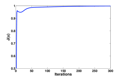
Figure 1: Training performance to find the optimal control strategy by maximizing $J(u)$ for the $V$-type quantum system with only uncertainty $g(\omega(t))$ where $\omega(t)\in[-0.28,0.28]$.

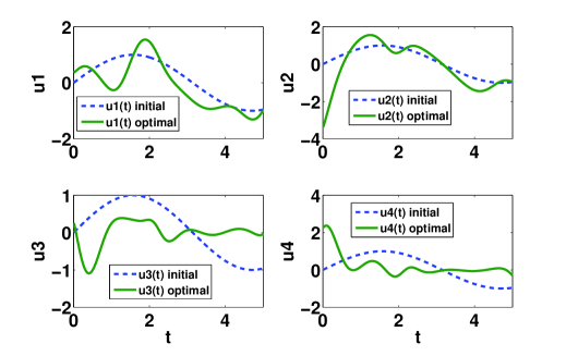
Figure 2: The learned optimal control strategy with maximized J(u) for the $V$-type quantum system with only uncertainty $g(\omega(t))$ where $\omega(t)\in[-0.28,0.28]$.

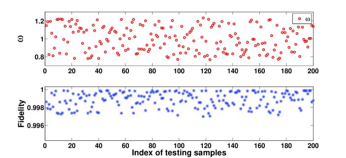
Figure 3: The testing performance (with respect to fidelity) of the learned optimal control strategy for the $V$-type quantum system with only uncertainty $g(\omega(t))$ where $\omega(t)\in[-0.28,0.28]$. For the 200 testing samples, the mean fidelity is 0.9989.

Now we consider the more general case that there exist uncertainties $g(\omega(t))$ and $f(\theta(t))$. Assume $\Omega=\Theta=0.28$, $g(\omega(t))=1-\omega\cos t$, $f(\theta(t))=1-\theta\cos t$ and both $\omega$ and $\theta$ have uniform distributions in the interval $[-0.28,0.28]$. To construct an augmented system for the training step, we have the training samples as follows

$$\left\{\begin{split}&g(\omega_{n})=1-0.28+\frac{0.28(2\text{fix}(n/7)-1)}{7},\\ &f(\theta_{n})=1-0.28+\frac{0.28(2\text{mod}(n,7)-1)}{7},\\ \end{split}\right.$$ (27)

where $n=1,2,\ldots,49$, $\text{fix}(x)=\max\{z\in\mathbb{Z}|z\leq x\}$, $\text{mod}(n,7)=n-7z(z\in\mathbb{Z}\ \text{and}\ \frac{n}{7}-1<z\leq\frac{n}{7})$ and $\mathbb{Z}$ is the set of integers. The training performance for this augmented system is shown in Fig. 4. The optimal control strategy is presented in Fig. 5. To test the optimal control strategy obtained from the training step using the augmented system, we randomly choose $200$ samples through sampling the uncertainties $g(\omega(t))$ and $f(\theta(t))$ whose control performance is presented in Fig. 6. The average fidelity is 0.9901. These numerical results show that the proposed SLC method using an augmented system for training is effective for control design of quantum systems with Hamiltonian uncertainties.

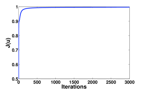
Figure 4: Training performance to find the optimal control strategy by maximizing $J(u)$ for the $V$-type quantum system with uncertainties $g(\omega(t))$ and $f(\theta(t))$ where $\omega(t)\in[-0.28,0.28]$ and $\theta(t)\in[-0.28,0.28]$.

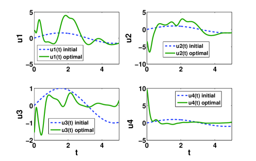
Figure 5: The learned optimal control strategy with maximized J(u) for the $V$-type quantum system with uncertainties $g(\omega(t))$ and $f(\theta(t))$ where $\omega(t)\in[-0.28,0.28]$ and $\theta(t)\in[-0.28,0.28]$.

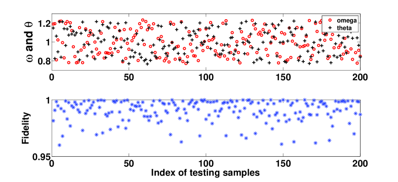
Figure 6: The testing performance (with respect to fidelity) of the learned optimal control strategy for the $V$-type quantum system with uncertainties $g(\omega(t))$ and $f(\theta(t))$ where $\omega(t)\in[-0.28,0.28]$ and $\theta(t)\in[-0.28,0.28]$. For the 200 testing samples, the mean fidelity is 0.9901.

V Conclusion

In this paper, we presented a systematic numerical methodology for control design of quantum systems with Hamiltonian uncertainties. The proposed sampling-based learning control method includes two steps of “training” and “testing and evaluation”. In the training step, the control is learned using a gradient flow based learning and optimization algorithm for an augmented system constructed from samples. In the process of testing and evaluation, the control obtained in the first step is evaluated for additional samples. The results show the effectiveness of the SLC method for control design of quantum systems with Hamiltonian uncertainties.

References

- [1] D. Dong, I.R. Petersen, “Quantum control theory and applications: A survey,” IET Control Theory & Applications, Vol.4, 2651-2671, 2010.
- [2] C. Altafini and F. Ticozzi, “Modeling and control of quantum systems: an introduction,” IEEE Transactions on Automatic Control, Vol. 57, No. 8, pp. 1898-1917, 2012.
- [3] H.M. Wiseman and G.J. Milburn, Quantum Measurement and Control, Cambridge, England: Cambridge University Press, 2010.
- [4] C. Brif, R. Chakrabarti and H. Rabitz, “Control of quantum phenomena: past, present and future,” New Journal of Physics, Vol. 12, p.075008, 2010.
- [5] M.A. Pravia, N. Boulant, J. Emerson, E.M. Fortunato, T.F. Havel, D.G. Cory and A. Farid, “Robust control of quantum information,” Journal of Chemical Physics, vol. 119, pp.9993-10001, 2003.
- [6] B. Qi, “A two-step strategy for stabilizing control of quantum systems with uncertainties,” Automatica, vol. 49, pp.834-839, 2013.
- [7] M.R. James, “Risk-sensitive optimal control of quantum systems”, Physical Review A, Vol. 69, p. 032108, 2004.
- [8] M.R. James, H.I. Nurdin and I.R. Petersen, “ control of linear quantum stochastic systems”, IEEE Transactions on Automatic Control, Vol. 53, pp. 1787-1803, 2008.
- [9] D. Dong and I.R. Petersen, “Sliding mode control of quantum systems”, New Journal of Physics, Vol. 11, p. 105033, 2009.
- [10] D. Dong and I.R. Petersen, “Sliding mode control of two-level quantum systems”, Automatica, Vol. 48, pp.725-735, 2012.
- [11] D. Dong and I.R. Petersen, “Notes on sliding mode control of two-level quantum systems”, Automatica, Vol. 48, pp.3089-3097, 2012.
- [12] C. Chen, D. Dong, J. Lam, J. Chu and T.J. Tarn, “Control design of uncertain quantum systems with fuzzy estimators,” IEEE Transactions on Fuzzy Systems, Vol. 20, No. 5, pp.820-831, 2012.
- [13] R. Long, G. Riviello and H. Rabitz, “The gradient flow for control of closed quantum systems”, IEEE Transactions on Automatic Control, in press, 2013.
- [14] J. Roslund and H. Rabitz, “Gradient algorithm applied to laboratory quantum control”, Physical Reveiw A, Vol. 79, p. 053417, 2009.
- [15] J. Zhang, L. Greenman, X. Deng, K.B. Whaley, “Robust control pulses design for electron shuttling in solid state devices,” arXiv:1210.7972, quant-ph, 2012.
- [16] C. Chen, D. Dong, R. Long, I.R. Petersen and H. Rabitz, “Sampling-based learning control of inhomogeneous quantum ensembles”, arXiv: 1308.1454 [quant-ph] 7 August 2013.
- [17] M.A. Nielsen and I.L. Chuang, Quantum Computation and Quantum Information, Cambridge, England: Cambridge University Press, 2000.
- [18] S.C. Hou, M.A. Khan, X.X. Yi, D. Dong and I.R. Petersen, “Optimal Lyapunov-based quantum control for quantum systems,” Physical Review A, Vol. 86, p. 022321, 2012.
- [19] J.Q. You and F. Nori, “Atomic physics and quantum optics using superconducting circuits,” Nature, Vol. 474, pp. 589-597, 2011.