Rotational microrheology of Maxwell fluids using micron-sized wires

Abstract

We demonstrate a simple method for rotational microrheology in complex fluids, using micrometric wires. The three-dimensional rotational Brownian motion of the wires suspended in Maxwell fluids is measured from their projection on the focal plane of a microscope. We analyze the mean-squared angular displacement of the wires of length between $1$ and $40\ \mu$m. The viscoelastic properties of the suspending fluids are extracted from this analysis and found to be in good agreement with macrorheology data. Viscosities of simple and complex fluids between $10^{-2}$ and $30$ Pa.s could be measured. As for the elastic modulus, values up to $\sim 5$ Pa could be determined. This simple technique, allowing for a broad range of probed length scales, opens new perspectives in microrheology of heterogeneous materials such as gels, glasses and cells.

I introduction

Microrheology consists in using microscopic probe particles embedded within a fluid to measure the relation between stress and deformationBreeveld and Pine (2003); Waigh (2005); Squires and Mason (2010a); Cicuta and Donald (2007). In passive microrheology, the linear viscoelastic properties of the fluid are derived from the thermal motion of the probes. In contrast, active microrheology involves forcing probes externally, and can be extended to the nonlinear regime of deformationZiemann et al. (1994); Cappallo et al. (2007); Dhar et al. (2010).

Microrheology experiments can be performed on small volumes, typically one microliter, which is essential when a limited amount of material is available, e.g. in biological samples. The technique was recently pushed to the limit, with less than one nanolitre available to investigate the beetle secretion Abou et al. (2010). Microrheology has opened up new fields of investigation in soft materials and complex fluids, including cellsHoffman et al. (2006); Weihs et al. (2006); MacKintosh and Schmidt (2010). By overcoming the limitations of traditional bulk rheology, it gives access to heterogeneities and an extended range of probed frequency and moduliWaigh (2005). Lastly, the technique has been used in out-of-equilibrium glasses, by combining passive and active methods to investigate deviations to fluctuation-dissipation relationsAbou and Gallet (2004); Jabbari-Farouji et al. (2007).

Most microrheology experiments are based on the investigation of the translational thermal motion of isotropic probes, typically spherical latex or silica colloids. In the case of anisotropic probes, the rotational motion becomes accessible as well. Despite recent developments in the synthesis of nano- and micrometric anisotropic particles Xia et al. (2003); Tang and Kotov (2005); Srivastava and Kotov (2009); Frka-Petesic et al. (2011), rotational microrheology has rarely been investigated. This comes mainly from the difficulty of recording the rotational thermal motion in three-dimension (3D) which requires advanced optical techniquesHan et al. (2006); Chang et al. (2010); Xiao et al. (2011). For instance, rotational Brownian motion was studied using light streak tracking of thin microdisks Cheng and Mason (2003), depolarized dynamic light scattering and epifluorescence microscopy of optically anisotropic spherical colloidal probes Andablo-Reyes et al. (2005); Anthony et al. (2006). It was also investigated with scanning confocal microscopy of colloidal rods with 3D resolution Mukhija and Solomon (2007), or reconstruction of the wire position from its hologram observed on the focal plane of a microscope Cheong and Grier (2010). Recently, we have proposed a method to measure the out-of-plane rotational motion of rigid wires, simply using 2D video microscopy Colin et al. (2012).

Anisotropic probes such as rigid wires present advantages over spherical probes. The translational Brownian motion of spherical probes up to $5\,\mu$m can typically be detected with standard video microscopy techniques. By comparison, we have previously shown that the translational and rotational diffusion of rigid wires up to $100\,\mu$m could be measuredColin et al. (2012). With rigid wires, the viscoelastic properties of materials such as actin networks Amblard et al. (1996); Lu and Solomon (2002) or cellsTseng et al. (2002); Hoffman et al. (2006), can be probed in a wide range of length scales, typically $1-100$ microns, giving a complete picture of the material. This is of importance in complex fluids which typically exhibit hierarchical structures on separate length scales.

In this paper, we demonstrate the ability of a recent technique for measuring the rotational thermal motion to probe the viscoelastic properties of complex fluids. The model complex fluids we used are wormlike micelle solutions, which are well characterized Maxwell fluidsLerouge and Berret (2010) and have been already investigated with other microrheology techniquesWilhelm et al. (2003); Buchanan et al. (2005); Willenbacher et al. (2007). Wires between $1$ and $40\,\mu$m in length are immersed in the Maxwell fluids with elastic moduli between $1-80$ Pa, and viscosities between $0.1-35$ Pa.s. The 3D rotational Brownian motion of the wires is extracted from their 2D projection on the focal plane of a microscope, following the procedure developed in Colin et al. (2012). The viscoelastic parameters of the Maxwell fluids, elastic modulus and static viscosity, are then deduced, and found in good agreement with the rheological measurements. The resolution of the method is shown to depend on the wire length.

II Rotational thermal motion of rigid wires: theory

The rotational Brownian motion of a rigid micrometric wire in a viscous fluid can be modeled by a Langevin equation describing the fluctuations of the wire orientation unit vector ${\bm{\hat{u}_{r}}}$. In the absence of an external torque, and neglecting inertia, the rotational equation of motion reads Doi and Edwards (1986):

$$\bm{0}=-{\zeta}_{R}\bm{\omega}+\bm{\Gamma_{r}}$$ (1)

in which ${\zeta}_{R}\bm{\omega}$ and ${\bm{\Gamma_{r}}}$ are respectively the viscous drag and the random Langevin torque. The projection of Eq. (1) along the vector $\bm{\hat{u}_{\theta}}$, leads to :

$${\zeta_{R}}^{\bot}\sin\theta\ \dot{\varphi}=\Gamma_{1}(t)$$ (2)

where $\Gamma_{1}(t)$ is the component of the random torque on vector $\bm{\hat{u}_{\theta}}$ and ${\zeta_{R}}^{\bot}$ the friction coefficient perpendicular to the wire axis. The spherical coordinates $\varphi(t)$ and $\theta(t)$ describe the wire orientationColin et al. (2012), and $\dot{\varphi}=d\varphi/dt$. The variable $\psi(t)$, defined as $\dot{\psi}=d\psi/dt=\sin\theta\ \dot{\varphi}$, obeys a one-dimensional Langevin equation (2) from which the mean-squared angular displacement (MSAD) is deduced :

$$\langle\Delta\psi^{2}(t)\rangle=2\frac{k_{B}\mathrm{T}}{{\zeta_{R}}^{\bot}}t=2D_{R}t$$ (3)

with $D_{R}$ the wire rotational diffusion coefficient and $k_{B}T$ the thermal energy.

For a cylindrical wire, length $L$ and diameter $d$, the perpendicular friction coefficient ${\zeta_{R}}^{\bot}$ can be expressed as :

$${\zeta_{R}}^{\bot}=\frac{\pi\eta L^{3}}{3\,g\left(L/d\right)}$$ (4)

where $g\left(L/d\right)$ is a dimensionless function of the aspect ratio $p=L/d$ and $\eta$ is the fluid viscosity. According to Tirado et al. (1984), we assume here that $g(p)=\ln(p)-0.662+0.917\,p-0.050\,p^{2}$, valid for $2<p<20$. The rotational diffusion coefficient $D_{R}$, deduced from Eqs. (3) and (4), writes:

$$D_{R}=\frac{3k_{B}\mathrm{T}}{\pi\eta L^{3}}g(L/d)$$ (5)

In a viscoelastic fluid, Eq. (2) is extended in a generalized Langevin equation :

$$\int_{-\infty}^{\infty}dt^{\prime}\zeta_{R}^{\bot}(t-t^{\prime})\dot{\psi}(t^{\prime})=\Gamma_{1}(t)$$ (6)

where $\zeta_{R}^{\bot}(t)$ is a delayed friction kernel which takes into account the fluid viscoelastic properties. The fluid is considered to be a linear viscoelastic material, where the coupling between translation and rotation is a negligible second order effectSquires and Mason (2010b). Considering that the surrounding stationary medium is in thermal equilibrium at temperature $T$, a Generalized Rotational Einstein Relation can be derived by analogy with the translational case Abou et al. (2008):

$$s^{2}\langle\hat{\Delta\psi^{2}}(s)\rangle=2k_{B}T/\hat{\zeta}_{R}^{\bot}(s)$$ (7)

In Eq. (7), $\langle\hat{\Delta\psi^{2}}(s)\rangle=\int_{0}^{\infty}\langle\Delta\psi^{2}(t)\rangle\mathrm{e}^{-st}\,\mathrm{d}t$ and $\hat{\zeta_{R}}^{\bot}(s)$ are the Laplace transform of the MSAD and the friction coefficient respectively. Assuming that Eq. (4) remains valid in the viscoelastic material, and can be extended to all frequencies $s$, the bulk frequency dependent viscosity $\hat{\eta}(s)$ is related to the friction coefficient according to :

$$\hat{\zeta_{R}}^{\bot}(s)=\frac{\pi\hat{\eta}(s)L^{3}}{3\,g\left(L/d\right)}$$ (8)

From Eqs. 7 and 8, the relation between the complex modulus $\hat{G}(s)=s\hat{\eta}(s)$ and the MSAD is :

$$s\langle\hat{\Delta\psi^{2}}(s)\rangle=\frac{6k_{B}T\,g\left(L/d\right)}{\pi L^{3}\hat{G}(s)}$$ (9)

In a Maxwell fluid, the complex modulus writes $\hat{G}(s)=\eta_{0}/(\tau_{R}+1/s)$, where $\eta_{0}=G_{0}\tau_{R}$ is the static viscosity, $\tau_{R}$ the relaxation time and $G_{0}$ the plateau modulus. This yields the expression of the MSAD in a Maxwell fluid :

$$\langle\Delta\psi^{2}(t)\rangle=\frac{6k_{B}T\,g\left(L/d\right)}{\pi L^{3}\eta_{0}}(t+\tau_{R})$$ (10)

The viscoelastic properties of the sample depend on the observation time scale. For $t\ll\tau_{R}$, the fluid behaves as an elastic solid and the MSAD approaches a constant limiting plateau value van Zanten and Rufener (2000):

$$\langle\Delta\psi^{2}(t\to 0)\rangle=\frac{6k_{B}T\,g\left(L/d\right)}{\pi L^{3}G_{0}}$$ (11)

For $t\gg\tau_{R}$, the fluid behaves as a viscous liquid and the mean-squared angular displacement increases linearly with time, with a slope proportional to $g(L/d)/L^{3}\eta_{0}$.

III Materials and Methods

III.1 Magnetic wires synthesis and characterization

The wires were formed by electrostatic complexation between oppositely charged nanoparticles and copolymers Fresnais et al. (2008); Yan et al. (2011). The particles were $8.3$ nm iron oxide nanocrystals ($\gamma-\mathrm{Fe}_{2}\mathrm{O}_{3}$, maghemite) synthesized by polycondensation of metallic salts in alkaline aqueous media Massart et al. (1995). To improve the colloidal stability, the cationic particles were coated with $M_{W}=2100\ \mathrm{g.mol}^{-1}$ poly(sodium acrylate) (Aldrich) using the precipitation-redispersion process Berret et al. (2007). This process resulted in the adsorption of a resilient $3$ nm polymer layer surrounding the particles. The copolymer used for the wire synthesis was poly(trimethylammoniumethylacrylate)-b-poly(acrylamide) with molecular weights $11000\ \mathrm{g.mol}^{-1}$ for the charged block and $30000\ \mathrm{g.mol}^{-1}$ for the neutral block Berret (2007). The applied protocol consisted first in the screening of the electrostatic interactions by bringing the polymer and particle dispersions to high salt concentration. In a second stage, the salt was progressively removed by dialysis. To stimulate their unidirectional growth, the particles and the polymers were co-assembled in the presence of a magnetic field of $0.1$ Tesla. The shelf life of the co-assembled structures is of the order of years. The wires are polydisperse. Their length distribution is described by a log-normal function with median length $L_{0}=27$ $\mu$m and polydispersity $s_{NW}=0.65$ . For this sample, the wires length varies between $1$ and $40$ $\mu$m. The average diameter $d$ of the wires is estimated at $400$ nm with scanning electron microscopyColin et al. (2012). Electrophoretic mobility and $\zeta-$potential measurements made with a Zeta sizer Nano ZS Malvern Instrument showed that the wires are electrically neutral Yan et al. (2011).

III.2 Maxwell fluids

Wormlike micellar solutions have received considerable attention during the past three decades because of their remarkable rheological properties Lerouge and Berret (2010). The surfactant solutions investigated here are binary mixtures made of cetylpyridinium chloride (CP⁺; Cl^-) and sodium salicylate (Na⁺; Sal^-) (abbreviated as CPCl/NaSal) dispersed in a $0.5$ M NaCl brine Berret et al. (1994); Walker et al. (1996). Since the pioneering work of Rehage and Hoffman, CPCl/NaSal is known to self-assemble spontaneously into micrometer long wormlike micellesRehage and Hoffmann (1988). Three CPCl/NaSal samples at concentration $c=1$ wt. $\%$, $c=2$ wt. $\%$ and $c=6$ wt. $\%$ were investigated in this work. These wormlike micelles build a semi-dilute entangled network that imparts to the solution a Maxwell viscoelastic behavior. In the semi-dilute regime, the mesh size of the network decreases as $c^{-0.65}$, in good agreement with theoretical expectationsCates (1987). It was found to be $35$ nm at $c=1$ wt. $\%$, and $15$ nm at $c=5$ wt. $\%$, i.e. much smaller than the wires smallest dimensionBerret et al. (1993).

III.3 Linear macrorheology

The complex viscoelastic modulus $G^{*}(\omega)=G^{\prime}(\omega)+iG^{\prime\prime}(\omega)$ of the wormlike micellar solutions was measured with a controlled shear rate rheometer (Physica MCR 500, cone and plate geometry). The measurements were carried out for angular frequencies in the range $\omega=0.1-100$ $\mathrm{rad.s}^{-1}$ in the linear regime (temperatures in the range $\mathrm{T}=20-25\,^{\circ}$C). A deformation of $10\%$ was applied to the samples at $c=2$ wt. $\%$ and $c=6$ wt. $\%$, while a $20\%$ deformation was applied to the sample at $c=1$ wt. $\%$. The viscoelastic response of CPCl/NaSal wormlike micelles was the one of a Maxwell fluid with a unique relaxation time $\tau_{R}$. The viscoelastic parameters $G_{0}$, $\tau_{R}$ and $\eta_{0}=\mathrm{lim}_{\omega\rightarrow 0⁡}|G^{*}(\omega)|/\omega$ were derived from the measurements.

III.4 Rotational particle tracking microrheology

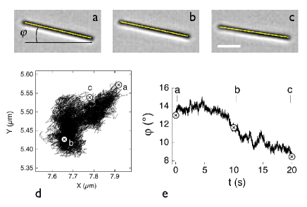
Figure 1: (a,b,c) Images of a $9.2\,\mu$m long wire immersed in a CPCl/NaSal wormlike micellar solution at $c=1$ wt. $\%$, at time intervals $0,10$ and $20$ s. (d) Brownian motion of the wire center-of-mass in the objective focal plane $(x,y)$. (e) The time dependence of the angle $\varphi(t)$, defined with respect to the horizontal axis, is extracted from the 2D images. The white scale bar is $5\,\mu$m long.

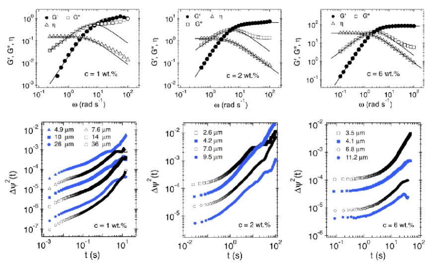
Figure 2: Macrorheology (top) and microrheology (bottom) experiments in the CPCl/NaSal micellar solutions at $c=1$ wt.$\%$ ($T=20\,^{\circ}$C), $c=2$ wt.$\%$ ($T=25\,^{\circ}$C) and $c=6$ wt.$\%$ ($T=25\,^{\circ}$C). Top: elastic modulus $G^{\prime}(\omega)$, loss modulus $G^{\prime\prime}(\omega)$, and magnitude of the complex viscosity $|\eta^{*}(\omega)|$. The solid lines correspond to the Maxwell model. Bottom: mean-squared angular displacement of wires immersed in the micellar solutions, as a function of the lag time. At short times, the MSADs exhibit a smooth increase (in the $c=1$ wt. $\%$) or a plateau (in the $c=2$ wt. $\%$ and $c=6$ wt. $\%$). This is followed by an increase at longer times in all cases. These two regimes are identified as Regime I and Regime II, respectively. The transition from Regime I to Regime II occurs at a lag time which is solution dependent. For the $c=1$ wt. $\%$, this lag time corresponds to the relaxation time $\tau_{R}$, whereas for the $c=2$ wt. $\%$ and $c=6$ wt. $\%$, it is the time where the MSAD reaches the resolution limit (see section IV).

The 2D projection of the wires thermal fluctuations on the focal plane of a microscope objective was recorded with a fast camera (EoSens Mikrotron). The camera is coupled to an inverted microscope (Leica DM IRB) with a $100\,\times$ oil immersion objective (NA$=1.3$). The objective temperature is controlled within $0.1\,^{\circ}$C using a Bioptechs heating ring coupled to a home-made cooling device. The sample temperature is controlled through the immersion oil in contact. The camera was typically recording $100$ images per second during $100$ s. The tracking of the wires was made at least $60\,\mu$m from the observation chamber walls, to minimize the interactions between walls and wires. To reduce the effect of hydrodynamic coupling, the wires concentration was chosen around $c=0.01$ wt. $\%$. Sedimentation of the wires was negligible on the recording time scales.

Fig. 1-a,b,c display a $9.2\,\mu$m long wire immersed in a CPCl/NaSal wormlike micellar solution at $c=1$ wt. $\%$, at time intervals $0,10$ and $20$ s. The wire orientation is determined by the angle $\varphi(t)$ defined with respect to the horizontal axis, and shown in Fig. 1-e. The Brownian motion of the wire center-of-mass is shown in Fig. 1-d. The 3D Brownian motion of the wire is extracted from its 2D projection on the $(x,y)-$plane, according the procedure described in Colin et al. (2012). The angle $\varphi(t)$ and the apparent length $L_{app}(t)$ are measured from the 2D images, using a homemade tracking algorithm implemented as an ImageJ plugin. The quantity $\Delta\psi(t)=\psi(t)-\psi(0)=\int_{0}^{t}dt^{\prime}\sin\theta(t^{\prime})\ \dot{\varphi}(t^{\prime})$, and subsequently the MSAD, $\langle\Delta\psi^{2}(t)\rangle$, reflecting the out-of-plane Brownian motion of the wires, are then computed from $\varphi(t)$ and $L_{app}(t)$. In Colin et al. (2012), the variable $\psi(t)$ was shown to correctly describe the 3D Brownian motion of the wires in a viscous liquid.

IV Results and discussion

IV.1 Macrorheology of wormlike micelles

Macrorheology experiments were performed on CPCl/NaSal solutions at concentration $c=1$ wt. $\%$, $c=2$ wt. $\%$ and $c=6$ wt. $\%$. At these concentrations, the micellar solutions are known to exhibit a Maxwell viscoelastic behaviorRehage and Hoffmann (1988); Berret et al. (1994), in agreement with the predictions of the Cates modelCates (1987). Fig. 2 (top) shows the elastic and loss moduli, $G^{\prime}(\omega)$ and $G^{\prime\prime}(\omega)$, and the magnitude of the complex viscosity, $|\eta^{*}(\omega)|$, for the different concentrations. The data were adjusted with the expressions corresponding to Maxwell fluids (solid lines), $G^{\prime}(\omega)/G_{0}=\omega^{2}\tau_{R}^{2}/(1+\omega^{2}\tau_{R}^{2})$, $G^{\prime\prime}(\omega)/G_{0}=\omega\tau_{R}/(1+\omega^{2}\tau_{R}^{2})$, and $|\eta^{*}(\omega)|=\eta_{0}/\sqrt{1+\omega^{2}\tau_{R}^{2}}$, with $\eta_{0}=G_{0}\tau_{R}$ the static viscosity.

The viscoelastic parameters, $G_{0}$, $\tau_{R}$ and $\eta_{0}$, obtained from the adjustments are shown in Table 1. They are in good agreement with macrorheology results published two decades agoBerret et al. (1994); Lerouge and Berret (2010). As seen in Fig. 2 (top), the linear viscoelastic responses of the $c=2$ wt. $\%$ and $c=6$ wt. $\%$ wormlike micelles are found to be purely that of Maxwell fluids Berret et al. (1994); Walker et al. (1996); Lerouge and Berret (2010), in the investigated frequency range. By comparison, in the $c=1$ wt. $\%$, slight deviations between the data and the Maxwell model are observed at high frequency, arising from additional relaxation mechanisms, such as the Rouse and breathing motions of the micellar chains Graneck and Cates (1992).

Table 1: Viscoelastic Maxwell parameters, $G_{0}$, $\tau_{R}$ and $\eta_{0}$, of the CPCl/NaSal micellar solutions (concentration $c$ in wt.), determined from macrorheology experiments.

Sample	$G_{0}$ (Pa)	$\tau_{R}$ (s)	$\eta_{0}$ (Pa.s)
$c=1\%$, $T=20\,^{\circ}$C	1.2 $\pm$ 0.2	0.12 $\pm$ 0.02	0.14 $\pm$ 0.05
$c=2\%$, $T=25\,^{\circ}$C	8.0 $\pm$ 0.3	0.21 $\pm$ 0.01	1.68 $\pm$ 0.05
$c=6\%$, $T=25\,^{\circ}$C	83 $\pm$ 1	0.42 $\pm$ 0.02	35 $\pm$ 1

IV.2 Rotational thermal motion of the wires

Microrheology experiments were carried out in the same micellar solutions. Fig. 2 (bottom) shows the MSADs of wires immersed in the micellar solutions, as a function of the lag time. At short times, the MSADs exhibit a slight increase (in the $c=1$ wt. $\%$) or a plateau (in the $c=2$ wt. $\%$ and $c=6$ wt. $\%$). This is followed by an increase at longer times in all cases. In the following, these two regimes will be identified as Regime I and Regime II, respectively. Before further analyzing the data, the angular resolution of the wire-based microrheology technique will be discussed.

IV.3 Angular resolution

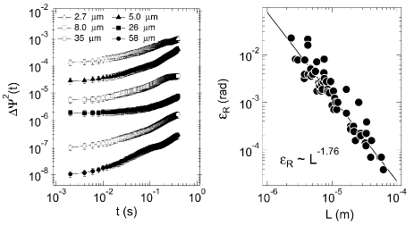
Figure 3: Angular resolution of the wire-based microrheology technique. Left: MSAD measured in a viscous liquid of high viscosity ($92$ vol.$\%$ glycerol/water solution, $\eta=0.45$ Pa.s, $T=25\,^{\circ}$C) for wires between $2$ and $58\,\mu$m, in the same experimental conditions as in the viscoelastic fluids. Due to the angular resolution limit, the MSAD exhibits a plateau at short displayed lag times. Right: angular resolution $\varepsilon_{R}$ as a function of the wire length.

The angular resolution was determined from the wires fluctuations in a viscous liquid of high viscosity $\eta$ ($92$ vol. $\%$ glycerol/water solution, $\eta=0.45$ Pa.s, $T=25\,^{\circ}$C). According to Eq. 3, the MSAD is expected to increase linearly with time. Fig. 3 (left) shows the MSAD for wires between $2$ and $58\,\mu$m. At short lag time, the MSAD exhibits a plateau due to the angular resolution limit, meaning that the minimum MSAD measurable with our setup is reached. Choosing a highly viscous fluid ensures that this limit will be reached within an accessible time.

Following the procedure developed for spherical probes Savin and Doyle (2005), the expression of the MSAD is extended asColin et al. (2012) :

$$\langle\Delta\psi^{2}(t,L)\rangle=\frac{6k_{B}T\,g\left(L/d\right)}{\pi L^{3}\eta}(t-\sigma/3)+2\,\varepsilon_{R}^{2}(L)\,,$$ (12)

which now includes the static error, $2\varepsilon_{R}^{2}(L)$, and the dynamic error accounting for the finite camera exposure time $\sigma$. The extrapolation $\langle\Delta\psi^{2}(t\to 0,L)\rangle=2\varepsilon_{R}^{2}(L)-2/3D_{R}(L)\,\sigma$ provides the minimum detectable mean-squared angular displacement. Since here $D_{R}\sigma/3\ll\varepsilon_{R}^{2}(L)$ on the entire range of $L$, this minimum reduces to $2\varepsilon_{R}^{2}(L)$.

Fig. 3 (right) shows $\varepsilon_{R}(L)$ as a function of the wire length $L$. It decreases with increasing length, as $2\times 10^{-12}L^{-1.76}$, with $\varepsilon_{R}$ in radian and $L$ in meter. This expression gives an idea of the angular resolution, $\sqrt{2}\varepsilon_{R}$, of our technique. It decreases from $1.3\,^{\circ}$ for $2\,\mu$m wires to $0.02\,^{\circ}$ for $20\,\mu$m wires. This yields a maximum measurable elastic modulus which depends on the wire length, as expressed in Eq. 11 when the MSAD reaches the resolution limit, $2\varepsilon_{R}^{2}(L)$. To give an order of magnitude, it corresponds to $2$ Pa for $2\,\mu$m wires and $12$ Pa for $20\,\mu$m wires. Longer wires will be more appropriate to study materials of high elastic moduli.

Knowing our technique limitation in $G_{0}$, and based on the macrorheology results described in section IV.1, only the elastic modulus $G_{0}$ of the $c=1$ wt. $\%$ CPCl/NaSal micellar solution can be determined with the wire-based microrheology technique. For the $c=2$ wt. $\%$ and $c=6$ wt. $\%$, the elastic modulus $G_{0}$ are beyond the resolution limit, Regime I reflects the angular resolution limit, and only Regime II will be analyzed.

IV.4 Microrheology of wormlike micelles

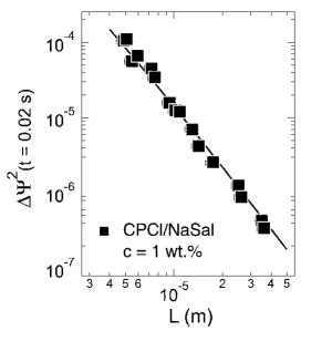
Figure 4: Microrheology in the $c=1$ wt $\%$ CPCl/NaSal micellar solution ($T=20\,^{\circ}$C). The mean-squared angular displacement in Regime I, $\langle\Delta\psi^{2}(t=0.02\,\rm{s})\rangle$, is plotted as a function of the wire length $L$. At leading order, it decreases as $L^{-3}$. The elastic plateau modulus $G_{0}=1.5\pm 0.5$ Pa is obtained by adjusting the data with Eq. 11, derived from the Maxwell model (solid line). It is in good agreement with the one measured with macrorheology, as shown in Table 1.

We now turn to the analysis of the MSAD measured in the micellar solutions (Fig. 2 (bottom)).

In Regime I of the $c=1$ wt $\%$ CpCl/NaSal solution, the MSADs extrapolated at $t\to 0$ were estimated as a function of the wire length. Fig. 4 shows a strong decrease of the data with increasing $L$. Using Eq. 11 to adjust the data in the form $\langle\Delta\psi^{2}(t\to 0)\rangle\sim g(L/d)L^{-3}/G_{0}$ (solid line), the elastic plateau modulus $G_{0}$ is deduced. Assuming an average diameter $d=400$ nm, least-square calculations provide $G_{0}=1.5\pm 0.5$ Pa compatible with macrorheology. Note that in the $c=1$ wt. $\%$ solution, the rather smooth plateau is the consequence of the extra Rouse and breathing modes previously mentioned Graneck and Cates (1992). In the $c=2$ wt $\%$ and $c=6$ wt $\%$ solutions, Regime I reflects the angular resolution limit, as shown in section IV.3.

At longer times (Regime II), an increase of the MSADs versus time is observed at all concentrations of the micellar solutions. The MSADs were adjusted using a power law of the form $\langle\Delta\psi^{2}(t)\rangle\sim t^{\alpha}$, $\alpha$ being an adjustable parameter. The distribution of the exponents $\alpha$ for the CPCl/NaSal solutions is shown in Figure 5 and compared to those found for a Newtonian fluid ($50$ vol. $\%$ glycerol/water mixture) where $\alpha$-values close to $1$ are expected. In both cases, the exponent distribution is peaked around $1$, with a similar polydispersity. These results evidence the existence of a diffusive regime in the rotational fluctuations of wires immersed in the micellar solutions.

Based on the exponent analysis, the MSAD in Regime II is adjusted according to $\langle\Delta\psi^{2}(t)\rangle=2D_{R}t$ extracted from Eq. 10. The rotational diffusion coefficient $D_{R}$ in the micellar solutions is shown in Fig. 6, as a function of the wire length. The results obtained in a water/glycerol mixture ($50$ vol. $\%$, $T=20\,^{\circ}$C) are also displayed. In all four fluids, the rotational diffusion coefficient $D_{R}$ is found to decrease with increasing length $L$. Using Eq. 5 to adjust the data in the form $D_{R}=3k_{B}Tg(L/d)L^{-3}/\pi\eta_{0}$ (solid lines), the static viscosity $\eta_{0}$ is extracted (Table 2). They are found to be in good agreement with the macroscopic rheology data, validating our wire-based microrheology technique.

In Fig. 2, the transition between Regime I and Regime II occurs at a lag time which is solution dependent. For the $c=1$ wt. $\%$, this lag time corresponds to the relaxation time $\tau_{R}$ (see Table 1), whereas for the $c=2$ wt. $\%$ and $c=6$ wt. $\%$, it is the time where the MSAD reaches the resolution limit.

Table 2: Static viscosities of the CPCl/NaSal solutions, and a glycerol/water mixture (($50$ vol.$\%$, $T=20\,^{\circ}$C) obtained from macrorheology (tabulated value for the glycerol/water mixture) and wire-based microrheology. The data obtained with both techniques are found to be in good agreement. The values are given in format mean $\pm$ standard deviation.

samples		$\eta_{0}$ (Pa.s)
		rheometer	wires
glycerol/water ($50$ vol.$\%$)		$0.0084$	$0.0090\pm 0.0003$
CPCl/NaSal	$c=1\,\%\ \mathrm{T}=20\,^{\circ}$C	$0.14\pm 0.05$	$0.20\pm 0.08$
	$c=2\,\%\ \mathrm{T}=25\,^{\circ}$C	$1.68\pm 0.05$	$1.7\pm 0.5$
	$c=6\,\%\ \mathrm{T}=25\,^{\circ}$C	$35\pm 1$	$26\pm 6$

Fig. 6 illustrates that $D_{R}(L)$ can be measured over at least $3$ decades yielding the same range in accessible viscosities. In our investigation, complex fluids with viscosities up to $\sim 30$ Pa.s could be measured. The dispersion of the data for $D_{R}(L)$, observed with respect to the fitting curves, is the consequence of the wire diameter distribution , as already seen in Newtonian fluids in Colin et al. (2012).

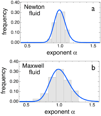
Figure 5: Exponent distribution: the MSADs were adjusted using a power law of the form $\langle\Delta\psi^{2}(t)\rangle\sim t^{\alpha}$, $\alpha$ being an adjustable parameter. The distribution of exponents $\alpha$ is shown in a) for a Newtonian fluid (water/glycerol mixture) in b) for the micellar solutions. In both cases, the exponent distribution is peaked around $1$, with a similar polydispersity. These results evidence the existence of a diffusive regime in the rotational fluctuations of wires immersed in the micellar solutions (Regime II).

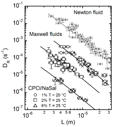
Figure 6: Rotational diffusion coefficient versus length, for wires dispersed in a water/glycerol mixture ($50$ vol.$\%$, $T=20\,^{\circ}$C) (labeled “Newton fluid”) and in the CPCl/NaSal micellar solutions (labeled “Maxwell fluids”). The data for $D_{R}$ in the micellar solutions were adjusted according to Eq. (5) (solid lines), with the static viscosity $\eta_{0}$ as a parameter ($d=400$ nm). The obtained values for $\eta_{0}$ are in good agreement with the macrorheology data, as shown in Table 2.

V Conclusion

In this paper, we demonstrate the ability of a wire-based rotational microrheology technique to probe the viscoelastic properties of complex fluids. Wires of $400$ nm in diameter and $1-40\,\mu$m in length were synthesized by electrostatic complexation. Passive microrheology was performed in CPCl/NaSal wormlike micellar solutions with Maxwellian behavior. The out-of-plane rotational Brownian motion of the wires was extracted from the 2D video microscopy images, following a method developed in Colin et al. (2012). The mean-squared angular displacement of wires between $1-40\,\mu$m was measured in the Maxwell fluids. Two regimes were identified. At short time, the MSAD exhibits a plateau or pseudo-plateau, which is followed by an increase at longer times. The first regime was shown to reveal the elastic plateau modulus in the Maxwell fluids with low elasticity such as the $c=1$ wt.$\%$ CPCl/NaSal micellar solution. In the $c=2$ wt.$\%$ and $c=6$ wt.$\%$ Maxwell fluids with higher elastic plateau modulus, it reflects the angular resolution limit. In the second regime, the MSAD was found to increase linearly, and was associated with a diffusive behavior. The values of the static viscosities could be deduced. All the values deduced from microrheology experiments, $G_{0}$ and $\eta_{0}$, were found to be in good agreement with macrorheology measurements. Elastic components up to $\sim 5$ Pa could be measured, higher elasticities falling beyond the resolution limit of the technique. Viscosities in the range $10^{-2}$ to $30$ Pa.s were also measured. All the rheological properties were found to be independent of the wire length.

Finally, we show here that micron-sized wires are efficient to probe the viscoelastic properties of complex fluids, and allow for the determination of both elastic and viscous components. With rigid wires, the viscoelastic properties of materials can be probed in a wide length scale range, typically $1-100\,\mu$mColin et al. (2012), giving a complete picture of the material. This is of importance in complex fluids which exhibit hierarchical structures on separate length scales, and could exhibit lengthscale-dependent rheology. This method broadens the array of tools available to microrheologists studying complex fluids. The range of measurable viscoelastic properties is similar to the one available with translational particle-tracking microrheology Waigh (2005). The main advantage of this technique is to increase by two orders of magnitude the range of accessible length scales, with a small number of probes involved compared to two-point microrheologyCrocker et al. (2000).

References

- Breeveld and Pine (2003) V. Breeveld and D. J. Pine, Journal of Materials Science 38, 4461 (2003).
- Waigh (2005) T. A. Waigh, Rep. Prog. Phys. 68, 685 (2005).
- Squires and Mason (2010a) T. M. Squires and T. G. Mason, Annual Review of Fluid Mechanics 42, 413 (2010a).
- Cicuta and Donald (2007) P. Cicuta and A. M. Donald, Soft Matter 3, 1449 (2007).
- Ziemann et al. (1994) F. Ziemann, J. O. Rädler, and E. Sackmann, Biophysical Journal pp. 2210–2216 (1994).
- Cappallo et al. (2007) N. Cappallo, C. Lapointe, D. H. Reich, and R. L. Leheny, Phys. Rev. E 76, 031505 (2007).
- Dhar et al. (2010) P. Dhar, Y. Y. Cao, T. M. Fischer, and J. A. Zasadzinski, Phys. Rev. Lett. 104, 104 (2010).
- Abou et al. (2010) B. Abou, C. Gay, B. Laurent, O. Cardoso, D. Voigt, H. Peisker, and S. Gorb, J. R. Soc. Interface 7, 1745 (2010).
- Hoffman et al. (2006) B. D. Hoffman, G. Massiera, K. M. V. Citters, and J. C. Crocker, Proceedings of the National Academy of Sciences 103, 10259 (2006).
- Weihs et al. (2006) D. Weihs, T. G. Mason, and M. A. Teitell, Biophysical Journal 91, 4296 (2006).
- MacKintosh and Schmidt (2010) F. C. MacKintosh and C. F. Schmidt, Current Opinion in Cell Biology 22, 29 (2010).
- Abou and Gallet (2004) B. Abou and F. Gallet, Phys. Rev. Lett. 93, 160603 (2004).
- Jabbari-Farouji et al. (2007) S. Jabbari-Farouji, D. Mizuno, M. Atakhorrami, F. C. MacKintosh, C. F. Schmidt, E. Eiser, G. H. Wegdam, and D. Bonn, Phys. Rev. Lett. 98, 108302 (2007).
- Xia et al. (2003) Y. Xia, P. Yang, Y. Sun, Y. Wu, B. Mayers, B. Gates, Y. Yin, F. Kim, and H. Yan, Advanced Materials 15, 353–389 (2003).
- Tang and Kotov (2005) Z. Tang and N. A. Kotov, Advanced Materials 17, 951–962 (2005).
- Srivastava and Kotov (2009) S. Srivastava and N. A. Kotov, Soft Matter 5, 1146 (2009).
- Frka-Petesic et al. (2011) B. Frka-Petesic, K. Erglis, J.-F. Berret, V. Cebers, A.; Dupuis, J. Fresnais, O. Sandre, and R. Perzynski, Journal of Magnetism and Magnetic Materials 323, 1309 (2011).
- Han et al. (2006) Y. Han, A. M. Alsayed, M. Nobili, J. Zhang, T. C. Lubensky, and A. G. Yodh, Science 314, 626 (2006).
- Chang et al. (2010) W.-S. Chang, J. W. Ha, L. S. Slaughter, and S. Link, Proc. Natl. Acad. Sci.. 107, 2781–2786 (2010).
- Xiao et al. (2011) L. Xiao, Y. Qiao, Y. He, and E. Yeung, Journal of the American Chemical Society 133, 10638 (2011).
- Cheng and Mason (2003) Z. Cheng and T. G. Mason, Phys. Rev. Lett. 90, 018304 (2003).
- Andablo-Reyes et al. (2005) E. Andablo-Reyes, P. Díaz-Leyva, and J. L. Arauz-Lara, Phys. Rev. Lett. 94, 106001 (2005).
- Anthony et al. (2006) S. M. Anthony, L. Hong, M. Kim, and S. Granick, Langmuir 22, 9812 (2006).
- Mukhija and Solomon (2007) D. Mukhija and M. J. Solomon, Journ. of Chem. Phys. 314, 98 (2007).
- Cheong and Grier (2010) F. C. Cheong and D. G. Grier, Opt. Express 18, 6555 (2010).
- Colin et al. (2012) R. Colin, M. Yan, L. Chevry, J.-F. Berret, and B. Abou, EPL (Europhysics Letters) 97, 30008 (2012).
- Amblard et al. (1996) F. Amblard, A. C. Maggs, B. Yurke, A. N. Pargellis, and S. Leibler, Phys. Rev. Lett. 77, 4470 (1996).
- Lu and Solomon (2002) Q. Lu and M. J. Solomon, Phys. Rev. E 66, 061504 (2002).
- Tseng et al. (2002) Y. Tseng, T. P. Kole, and D. Wirtz, Biophysical Journal 83, 3162 (2002).
- Lerouge and Berret (2010) S. Lerouge and J.-F. Berret, in Polymer characterization: rheology, laser interferometry, electrooptics, Advances in polymer science, edited by K. Dusek and J.-F. Joanny (2010), vol. 230, pp. 1–71.
- Wilhelm et al. (2003) C. Wilhelm, J. Browaeys, A. Ponton, and J.-C. Bacri, Phys. Rev. E 67, 011504 (2003).
- Buchanan et al. (2005) M. Buchanan, M. Atakhorrami, J. F. Palierne, and C. F. Schmidt, Macromolecules 38, 8840 (2005).
- Willenbacher et al. (2007) N. Willenbacher, C. Oelschlaeger, M. Schopferer, P. Fischer, F. Cardinaux, and F. Scheffold, Phys. Rev. Lett. 99, 068302 (2007).
- Doi and Edwards (1986) M. Doi and S. F. Edwards, Theory of polymer dynamics (Oxford University Press, 1986).
- Tirado et al. (1984) M. Tirado, C. L. Martinez, and J. García de la Torre, Journ. of Chem. Phys. 81, 2047 (1984).
- Squires and Mason (2010b) T. M. Squires and T. G. Mason, Rheologica Acta 49, 1165 (2010b).
- Abou et al. (2008) B. Abou, F. Gallet, P. Monceau, and N. Pottier, Physica A 387, 3410 (2008).
- van Zanten and Rufener (2000) J. H. van Zanten and K. P. Rufener, Physical Review E 62, 5389 (2000).
- Fresnais et al. (2008) J. Fresnais, J.-F. Berret, B. Frka-Petesic, O. Sandre, and R. Perzynski, Advanced Materials 20, 3877–3881 (2008).
- Yan et al. (2011) M. Yan, J. Fresnais, S. Sekar, J.-P. Chapel, and J.-F. Berret, ACS Applied Materials & Interfaces 3, 1049 (2011).
- Massart et al. (1995) R. Massart, E. Dubois, V. Cabuil, and E. Hasmonay, Journal of Magnetism and Magnetic Materials 149, 1 (1995).
- Berret et al. (2007) J.-F. Berret, O. Sandre, and A. Mauger, Langmuir 23, 2993 (2007).
- Berret (2007) J.-F. Berret, Macromolecules 40, 4260 (2007).
- Berret et al. (1994) J.-F. Berret, D. C. Roux, and G. Porte, Journal de Physique (II) France 4, 1261 (1994).
- Walker et al. (1996) L. M. Walker, P. Moldenaers, and J.-F. Berret, Langmuir 12, 6309 (1996).
- Rehage and Hoffmann (1988) H. Rehage and H. Hoffmann, The Journal of Physical Chemistry 92, 4712 (1988).
- Cates (1987) M. E. Cates, Macromolecules 20, 2289 (1987).
- Berret et al. (1993) J.-F. Berret, J. Apell, and G. Porte, Langmuir 9, 2851 (1993).
- Graneck and Cates (1992) R. Graneck and M. E. Cates, J. Chem. Phys. 96, 4758 (1992).
- Savin and Doyle (2005) T. Savin and P. Doyle, Biophysical Journal 88, 623 (2005).
- Crocker et al. (2000) J. C. Crocker, M. Valentine, E. R. Weeks, T. Gisler, P. D. Kaplan, A. G. Yodh, and D. A. Weitz, Phys. Rev. Lett. 85, 888 (2000).