Multiple-choice Vector Bin Packing:
Arc-flow Formulation with Graph Compression

Abstract

The vector bin packing problem (VBP) is a generalization of bin packing with multiple constraints. In this problem we are required to pack items, represented by $p$-dimensional vectors, into as few bins as possible. The multiple-choice vector bin packing (MVBP) is a variant of the VBP in which bins have several types and items have several incarnations. We present an exact method, based on an arc-flow formulation with graph compression, for solving MVBP by simply representing all the patterns in a very compact graph. As a proof of concept we report computational results on a variable-sized bin packing data set.  
Keywords: Multiple-choice Vector Bin Packing, Arc-flow Formulation, Integer Programming.

1 Introduction

The vector bin packing problem (VBP), also called general assignment problem by some authors, is a generalization of bin packing with multiple constraints. In this problem, we are required to pack $n$ items of $m$ different types, represented by $p$-dimensional vectors, into as few bins as possible. The multiple-choice vector bin packing problem (MVBP) is a variant of VBP in which bins have several types (i.e., sizes and costs) and items have several incarnations (i.e., will take one of several possible sizes); this occurs typically in situations where one of several incompatible decisions has to be taken (see, e.g., Patt-Shamir and Rawitz, 2012).

Brandão and Pedroso, (2013) present a general arc-flow formulation with graph compression for vector packing. This formulation is equivalent to the model of Gilmore and Gomory, (1963), thus providing a very strong linear relaxation. It has proven to be very effective on a large variety of problems through reductions to vector packing. In this paper, we apply the general arc-flow formulation to the multiple-choice vector packing problem.

The remainder of this paper is organized as follows. Section 2 presents the arc-flow formulation for MVBP. Some computational results are presented in Section 3 and Section 4 presents the conclusions.

2 Arc-flow formulation with graph compression for MVBP

In order to solve a cutting/packing problem, the arc-flow formulation proposed in Brandão and Pedroso, (2013) only requires the corresponding directed acyclic multigraph $G=(V,A)$ containing every valid packing pattern represented as a path from the source to the target. In order to model MVBP, we will start by defining the underlying graph.

For a given $i$, let $\mathbf{J}_{i}$ be the set of incarnations of item $i$, and let $\mathbf{I}=\{(i,j):i=1..m,j\in\mathbf{J}_{i}\}$ be the set of items. Let $it_{i}^{j}=(i,j)\in\mathbf{I}$ be the incarnation $j$ of item $i$ and $w(it_{i}^{j})$ its weight vector. For the sake of simplicity, we define $it_{0}^{0}$ as an item with weight zero in every dimension; this artificial item is used to label loss arcs. Let $b_{i}$ be the demand of items of type $i$, for $i=1,\ldots,m$. Let $q$ be the number of bin types. Let $W(t)$ and $C(t)$ be the capacity vector and the cost of bins of type $t$, respectively.

Example 1

Figure 1 shows the graph associated with a two dimensional ($p=2$) instance with bins of two types ($q=2$). The bins of type 1 have capacity $W(1)=(100,75)$ and cost $C(1)=3$. The bins of type 2 have capacity $W(2)=(75,50)$ and cost $C(2)=2$. There are three items ($n=3$) to pack of two different types ($m=2$). The first item type has demand $b_{1}=2$, and a single incarnation with weight $w(it_{1}^{1})=(75,50)$. The second item type has demand $b_{2}=1$, and two incarnations with weights $w(it_{2}^{1})=(40,15)$ and $w(it_{2}^{2})=(25,25)$.

We need to build a graph for each bin type considering every item incarnation as a different item. The arc-flow graphs must contain every valid packing pattern represented as a path from the source to the target, and they may not contain any invalid pattern. These graphs – say, $G_{1},\ldots,G_{t}$ – can be built using the step-by-step algorithm proposed in Brandão, (2012) or the algorithm proposed in Brandão and Pedroso, (2013) (recommended for efficiency). Both algorithms perform graph compression and hence the resulting graphs tend to be small.

Figure 1 shows an arc-flow graph for Example 1. Paths from $\textsc{s}_{t}$ to $\textsc{t}_{t}$ represent every valid pattern for bins of type $t$, for $t=1,\ldots,q$. Each of these subgraphs is built considering every item incarnation as a different item. We connect a super source node s to every $\textsc{s}_{t}$, and every $\textsc{t}_{t}$ to a super target node t. Paths from s to t represent every valid packing pattern using any bin type.

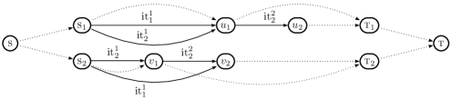
Figure 1: Arc-flow graph containing every valid packing pattern for Example 1.

Paths from $\textsc{s}_{t}$ to $\textsc{t}_{t}$ represent every valid pattern for bins of type $t$, for each $t$. Paths from s to t represent every valid packing pattern using any bin type.

Graphs $G_{1},\ldots,G_{t}$ are already compressed, but in order to reduce the whole graph size even more, we apply again to $G$ the final compression step of the method proposed in Brandão and Pedroso, (2013). Note that this compression step can only be applied if the set of item incarnations does not depend on the bin type. We relabel the graph using the longest paths from the source in each dimension. Let ($\psi^{1}(v)$, $\psi^{2}(v)$, …, $\psi^{p}(v)$) be the label of node $v$ in the final graph, where

$$\psi^{d}(v) = \left\{\begin{array}[]{ll}0&\mbox{if }v=\textsc{s},\\ \max_{(u,v^{\prime},it_{i}^{j})\in A:v^{\prime}=v}\{\psi^{d}(u)+w(it_{i}^{j})^{d}\}&\mbox{otherwise.}\\ \end{array}\right.$$ (3)

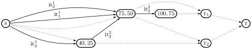
Figure 2: After applying the final compression step to the graph of Figure 1.

The final compression step removed 3 vertices and 3 arcs on this small example.

The final graph may contain parallel arcs for different incarnations of the same item. Since having multiple parallel arcs for the same item is redundant, only one of them is left.

The arc-flow formulation for multiple-choice vector bin packing is the following:

minimize $$\sum_{t=0}^{q}C(t)f_{\textsc{t}_{t},\textsc{t},it_{0}^{0}}$$ (4)

subject to $$\sum_{(u,v,it)\in A:v=k}f_{u,v,it}\hskip 8.53581pt-\sum_{(v,r,it)\in A:v=k}f_{v,r,it}= \left\{\begin{array}[]{rl}-z&\mbox{if }k=\textsc{s},\\ z&\mbox{if }k=\textsc{t},\\ 0&\mbox{for }k\in V\setminus\{\textsc{s},\textsc{t}\},\\ \end{array}\right.$$ (8)

$$\sum_{(u,v,it_{i}^{j})\in A:i=k}f_{u,v,it_{i}^{j}}\geq b_{k}, k\in\{1,\ldots,m\}\setminus J,$$ (9)

$$\sum_{(u,v,it_{i}^{j})\in A:i=k}f_{u,v,it_{i}^{j}}=b_{k}, k\in J,$$ (10)

$$f_{u,v,it_{i}^{j}}\leq b_{i}, \forall(u,v,it_{i}^{j})\in A,\mbox{ if }i\neq 0,$$ (11)

$$f_{u,v,it_{i}^{j}}\geq 0,\mbox{ integer}, \forall(u,v,it_{i}^{j})\in A,$$ (12)

where $z$ can be seen as a feedback from t to s; $m$ is the number of different items; $q$ is the number of bin types; $b_{i}$ is the demand of items of type $i$; $V$ is the set of vertices, s is the source vertex and t is the target; $A$ is the set of arcs, where each arc has three components $(u,v,it_{i}^{j})$ corresponding to an arc between nodes $u$ and $v$ that contributes to the demand of items of type $i$; arcs $(u,v,it_{0}^{0})$ are loss arcs; $f_{u,v,it}$ is the amount of flow along the arc $(u,v,it)$; and $J\subseteq\{1,\ldots,m\}$ is a subset of items whose demands are required to be satisfied exactly for efficiency purposes. For having tighter constraints, one may set $J=\{i=1,\ldots,m:b_{i}=1\}$ (we have done this in our experiments). The main difference between this and the original arc-flow formulation is the objective function.

Algorithm 1 illustrates our solution method. More details on algorithms for graph construction and solution extraction are given in Brandão and Pedroso, (2013) and Brandão, (2012).

1

2

3

input :  $\mathbf{I}$ - set of items; $m$ - number of different items; $w(it_{i}^{j})$ - weight vector of the incarnation $j$ of item $i$; $b_{i}$ - demand of item $i$; $q$ - number of bin types; $W(t)$, $C(t)$ - capacity and cost of bins of type $t$, respectively;

output : MVBP Solution

4

5function $\textnormal{{solveMVBP}}(\mathbf{I},m,w,b,q,W,C)$:

6       $V,A\leftarrow(\{\textsc{s},\textsc{t}\},\emptyset)$;

7       for $t\leftarrow 1$ to $q$ do // for each bin type $t$

8             $\textnormal{{labels}}\leftarrow\mathbf{I}$;

9             $\textnormal{{weight}}\leftarrow[w(it_{i}^{j}):it_{i}^{j}\in\mathbf{I}]$;

10             $\textnormal{{demand}}\leftarrow[b_{i}:it_{i}^{j}\in\mathbf{I}]$;

             $(G_{t},\textsc{s}_{t},\textsc{t}_{t})\leftarrow\textnormal{{buildGraph}}(m,\textnormal{{labels}},\textnormal{{weight}},\textnormal{{demand}},W(t))$;

              // build the arc-flow graph $G_{t}$ for bins of type $t$

11             $(V_{t},A_{t})\leftarrow G_{t}$;

12             $V\leftarrow V\cup V_{t}$;

13             $A\leftarrow A\cup A_{t}\cup\{(\textsc{s},\textsc{s}_{t},it_{0}^{0}),(\textsc{t}_{t},\textsc{t},it_{0}^{0})\}$;

14            

15      $G\leftarrow(V,A)$;

       $G\leftarrow\textnormal{{compress}}(G)$;

        // apply the final compression step to $G$

       $f\leftarrow\textnormal{{MIPSolver}}(\mbox{arc-flow model},q,C,G,b)$;

        // solve the arc-flow model over $G$

       return $\textnormal{{extractSolution}}(f)$;

        // extract the MVBP solution from the arc-flow solution

16      

17

Algorithm 1 MVBP Solution Method

3 Computational results

As a proof of concept, we used to the arc-flow formulation to solve variable-sized bin packing. A specific method for solving this problem has been presented in Alves and Valério de Carvalho, (2007); here we proposed to simply model it as a unidimensional multiple-choice vector bin packing problem. We solved the benchmark data set of Monaci, (2001), which is composed of 300 instances. In this data set, the items sizes were randomly generated within three different ranges: $w_{i}\in[1,100]$ (X=1), $w_{i}\in[20,100]$ (X=2) and $w_{i}\in[50,100]$ (X=3). There are instances with three ($q=3$) and five $(q=5)$ bin types; the bin sizes are $[100,120,150]$ for $q=3$ and $[60,80,100,120,150]$ for $q=5$. For each range and each number of bin types, there are 10 instances for each $n\in\{25,50,100,200,500\}$. The average run time on the 300 instances was less than 1 second and none of these instances took longer than 6 seconds to be solved exactly.

Table 1 presents the results. The meaning of each column is as follows: $q$ - number of different bin types; $n$ -  total number of items; $m$ - number of different items; $\#v$, $\#a$ - number of vertices and arcs in the final arc-flow graph; $\%v,\%a$ - percentage of vertices and arcs removed by the final compression step; $t^{\mathop{\mathrm{ip}}}$ - time spent solving the model; $n^{\mathop{\mathrm{bb}}}$ - average number of nodes explored in the branch-and-bound procedure; $t^{\mathop{\mathrm{tot}}}$ - run time in seconds. The values shown are averages over the 10 instances in each class.

CPU times were obtained using a computer with two Quad-Core Intel Xeon at 2.66GHz, running Mac OS X 10.8.5. The graphs for each bin type were generated using the algorithm proposed in Brandão and Pedroso, (2013), which was implemented in C++, and the final model was produced using Python. The models were solved using Gurobi 5.5.0 (Gu et al., 2013), a state-of-the-art mixed integer programming solver. The parameters used in Gurobi were Threads = 1 (single thread), Presolve = 1 (conservative), Method = 2 (interior point methods), MIPFocus = 1 (feasible solutions), Heuristics = 1, MIPGap = 0, MIPGapAbs = $1-10^{-5}$ and the remaining parameters were Gurobi’s default values. The branch-and-cut solver used in Gurobi uses a series of cuts; in our models, the most frequently used were Gomory, Zero half and MIR. The source code is available online.

[b] Range $q$ $n$ $m$ $\#v$ $\#a$ $\%v$ $\%a$ $n^{\mathop{\mathrm{bb}}}$ $t^{\mathop{\mathrm{ip}}}$ $t^{\mathop{\mathrm{tot}}}$ X=1 3 25 22.0 71.1 616.9 41.90 13.68 13.5 0.15 0.23 X=1 3 50 38.3 115.1 1,641.7 53.38 26.39 7.2 0.56 0.69 X=1 3 100 62.3 134.3 3,128.8 56.89 38.49 3.2 1.70 1.94 X=1 3 200 86.8 142.9 4,930.3 57.86 43.33 0.0 1.35 1.72 X=1 3 500 98.8 148.3 6,047.9 58.34 46.07 0.0 1.41 1.91 X=1 5 25 22.4 91.8 807.8 48.64 16.40 0.0 0.11 0.21 X=1 5 50 39.1 122.9 1,947.6 60.62 27.83 0.8 0.57 0.73 X=1 5 100 61.8 139.3 3,518.9 66.12 40.94 0.0 0.73 1.01 X=1 5 200 85.6 147.1 5,289.6 68.06 48.89 0.0 2.19 2.62 X=1 5 500 98.5 151.9 6,459.6 69.02 52.91 0.0 1.26 1.85 X=2 3 25 21.6 38.4 307.0 35.46 10.27 0.0 0.04 0.10 X=2 3 50 36.9 72.8 1,020.7 43.19 10.25 0.0 0.12 0.21 X=2 3 100 58.7 96.0 2,379.0 50.36 13.30 0.0 0.33 0.49 X=2 3 200 73.1 108.7 3,554.2 53.70 16.11 0.0 0.67 0.90 X=2 3 500 80.0 113.3 4,076.2 54.39 17.39 0.0 0.41 0.68 X=2 5 25 22.2 43.3 348.7 39.33 11.63 0.0 0.02 0.09 X=2 5 50 37.4 75.3 1,037.8 46.88 10.82 0.0 0.09 0.20 X=2 5 100 57.5 96.0 2,275.6 54.26 13.10 0.0 0.30 0.47 X=2 5 200 73.7 110.2 3,757.8 59.99 17.17 0.0 0.49 0.75 X=2 5 500 79.7 115.5 4,267.1 60.94 18.75 0.0 0.84 1.20 X=3 3 25 19.4 15.6 90.4 16.69 3.48 0.0 0.00 0.06 X=3 3 50 30.7 22.8 148.0 12.69 2.78 0.0 0.01 0.07 X=3 3 100 44.8 36.5 228.0 7.86 1.35 0.0 0.01 0.07 X=3 3 200 49.3 41.9 254.8 6.69 1.16 0.8 0.01 0.08 X=3 3 500 50.0 43.0 260.0 6.52 1.14 0.0 0.01 0.07 X=3 5 25 18.5 18.2 101.0 25.03 6.82 0.0 0.00 0.06 X=3 5 50 31.6 26.3 179.8 20.14 4.83 0.0 0.00 0.08 X=3 5 100 43.3 36.5 251.1 15.62 3.23 0.0 0.01 0.08 X=3 5 200 49.5 44.4 297.9 13.62 2.65 0.0 0.01 0.09 X=3 5 500 50.0 45.0 301.0 13.46 2.59 0.0 0.01 0.12

Table 1: Results for variable-sized bin packing.

4 Conclusions

We propose an arc-flow formulation with graph compression for solving multiple-choice vector bin packing problems. This formulation is simple and proved to be effective for solving variable-sized bin packing as a unidimensional multiple-choice vector packing problem. This paper shows the flexibility and effectiveness of the general arc-flow formulation with graph compression for modeling and solving cutting and packing problems, beyond those solved through reductions to vector packing in the original paper.

References

- Alves and Valério de Carvalho, (2007) Alves, C. and Valério de Carvalho, J. (2007). Accelerating column generation for variable sized bin-packing problems. European Journal of Operational Research, 183(3):1333 – 1352.
- Brandão, (2012) Brandão, F. (2012). Bin Packing and Related Problems: Pattern-Based Approaches. Master’s thesis, Faculdade de Ciências da Universidade do Porto, Portugal.
- Brandão, (2013) Brandão, F. (2013). VPSolver: Arc-flow Vector Packing Solver, Version 1.1. (Software program).