Aspects of line operators of class ${\cal S}$ theories

Abstract:

Geometric picture of line operators of $\mathcal{N}=2$ class ${\cal S}$ theories was found by imposing closure condition on operator product expansion (OPE) of line operators. In this paper, we first identify the geometric representation of ordinary Wilson-’t Hooft line operators of field theory, and study duality action on them. We further define a Dirac product between line operators and classify the allowed set of line operators by requiring: a: closure of OPE; b: mutual locality; c: maximality. Using above classifications, we find many distinct gauge theories associated with a single duality frame, and show explicitly that new possibilities correspond to the choice of global form of gauge group and discrete $\theta$ angles. We also study S and T duality actions relating those theories. In particular, we find very interesting duality webs for Maldacena-Nunez theory.

1 Introduction

Wilson and ’t Hooft line operators are important extended physical observables for gauge theory: they can be used to probe the phases of field theory; the study of duality actions on line operators reveals many important property of dualities, etc.

We are interested in studying line operators of four dimensional $\mathcal{N}=2$ class ${\cal S}$ theory which includes Lagrangian theory and non-Lagrangian theory such as Argyres-Douglas theory[1, 2]. The study of of this class of theories can provide invaluable insights into the dynamics of quantum field theory.

$\mathcal{N}=2$ class ${\cal S}$ theory is defined by compactifying 6d $(2,0)$ theory on a Riemann surface with various co-dimensional two defects [3, 4, 5, 6]. One of really remarkable thing about this type of construction is that various highly non-trivial properties of field theory is mapped to the study of simple geometric objects on Riemann surface. For instance, the construction of new theories becomes the study of local punctures; duality actions of field theory [7] are simply the mapping class group actions of Riemann surface [3], etc.

For our interest, line operator of class ${\cal S}$ theory defined using $A_{1}$ theory is related to the closed curves on Riemann surface [8, 9], which is a natural set of objects on which mapping class group action acts [10]. Things become even more interesting if we consider higher rank theory. Using closure of operator product expansion (OPE) defined between the line operators, it is found that the web structure is needed for geometric representation of general line operators of higher rank theory [11] .

In this paper, we further study line operators of class ${\cal S}$ theory using the geometric picture developed in [11], and our main results are summarized as follows:

• Geometric objects corresponding to general Wilson-’t Hooft line operators found in [19] are identified. Such correspondence is achieved by taking a weakly coupled duality frame and using Dehn-Thurston coordinates for the closed curves. The crucial thing is that web structure is needed to describe general Wilson-’t Hooft line operators. We give the formula for $T$ and $S$ transformation on line operators represented by closed curves.

• We define a Dirac product and mutual locality condition between line operators using cluster coordinates. We also give a simple geometric interpretations of Dirac product using intersection form of the corresponding homology class, and mutual locality condition becomes a constraint on homology class whose study is much more simpler than line operator itself which is classified by homotopy theory.

• We classify the allowed set of line operators by imposing following three conditions: a: closure of OPE; b: mutual locality; c: maximality. We identify the corresponding global form of the gauge group and discrete $\theta$ angles. The effect of those discrete $\theta$ angles on line operators are studied in a beautiful paper [20] generalizing earlier analysis [9], our results are a further generalization to theory with more gauge groups with fundamental matter (see also [18] for a similar study of these $\theta$ angles using 6d theory.).

• We study the duality action on homology class, and then relate theories with different gauge groups and $\theta$ angles. See figure. 1 for an example.

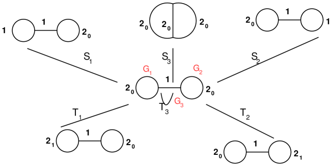
Figure 1: Duality action relating different gauge theory defined using genus two Riemann surface. Here 1 means that gauge group is $SU(2)$, $2_{0}$ means the gauge group is $SU(2)/Z_{2}$, and $2_{1}$ means the gauge group is also $SU(2)/Z_{2}$, but there is a discrete $\theta$ angle associated with it. $S_{i}$ is the S duality transformation on gauge group and $T_{i}$ is the $T$ transformation.

This paper is summarized as follows: in section 2, we review the geometric picture of line operators found in [11], and the important objects are closed curves associated with homotopy class and the webs. In section 3, we identify the Wilson-’t Hooft line operators in field theory with the geometric objects reviewed in section 2. Section 4 discusses the definition of Dirac product and the importance of intersection form of homology class. Section 5 focuses on the classification of allowed set of line operators using homology theory, and we also study the duality actions relating different theories. Finally, a short conclusion is given.

2 Closure of OPE: web structure

2.1 Geometric picture

Let’s first review the geometric construction of half-BPS line operators of $\mathcal{N}=2$ class ${\cal S}$ theory found in [11] (see [8, 9] for the discussion of $A_{1}$ theory). Class ${\cal S}$ theory is engineered by compactifying six dimensional $(2,0)$ theory on a Riemann surface $\Sigma$ with regular and irregular singularities, see [3, 4, 5, 6] for detailed properties of these singularities. In this paper, we only consider 4d theory engineered using 6d $(2,0)$ $A_{N-1}$ type theory, and only consider full regular and irregular punctures.

For our later purpose, the punctured Riemann surface could be replaced by a bordered Riemann surface by replacing irregular singularity with a disc with marked points [21], and the number of marked points depend on the specific type of irregular singularity. Therefore the geometric avatar for our study is a bordered Riemann surface $\Sigma_{(b_{1},b_{2},\ldots,b_{i}),n}$ , where $n$ is the number of punctures (regular singularity), and $b_{1}$ is the number of marked points on the boundary of the first disc, $b_{2}$ is the number of marked points on the boundary of the second disc, etc.

Elementary half-BPS line operator of class ${\cal S}$ theory are formed by wrapping half-BPS co-dimension four surface operator of $(2,0)$ theory on closed curves on $\Sigma$. These surface operators could be thought of as the boundary of M2 brane ending on M5 brane. After wrapping the surface operator on closed curves of Riemann surface, we get a one dimensional object in 4d which is then identified as line operator of four dimensional theory. We simply assume that all line operators in 4d are parallel straight lines, and the classification would become the classification of closed curves on $\Sigma$. See figure. 2.

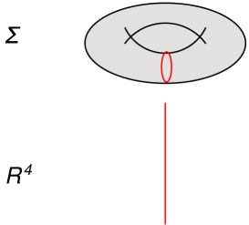
Figure 2: A surface operator of 6d $(2,0)$ theory is wrapped on a closed curve on Riemann surface and becomes line operator of 4d theory.

As shown in [22, 23, 24], half-BPS surface operator is classified by irreducible representation of $su(N)$. So if we consider a single closed curve, then the possible 4d line operator one can find from wrapping surface operator is classified by the irreducible representation of $su(N)$ Lie algebra. The unique highest weight of an irreducible representation can be expanded as

$$R=\sum n_{i}\omega_{i},$$ (1)

here $\omega_{i}$ is the fundamental weight. Motived by this fact, we can first represent a line operator in fundamental representation $w_{i}$ by a closed curve with label $i$, and call these labeled curves as colored closed curves. Then we can represent a general line operator in representation $R$ by a set of colored closed curves, and the multiplicity for color $i$ curves is $n_{i}$, see left of figure. 3.

A general line operator formed by half-BPS surface operator is then represented by a set of non-intersecting colored closed curves with positive integer weights, and those geometric objects are called colored A lamination:

Definition: A integral colored A-lamination on a bordered Riemann surface is a homotopy class of a collection of finite number of self- and mutually nonintersecting colored unoriented curves either closed or connecting two points of the boundary disjoint from marked points with integral weights and subject to the following conditions and equivalence relations:

(1) Weights of all colored curves are positive, unless a curve is special .

(2) A lamination containing a curve of weight zero is considered to be equivalent to the lamination with this curve removed.

(3) A lamination containing a contractible curve is considered to be equivalent to the lamination with this curve removed.

(4) A lamination containing two homotopy equivalent curves with same color $i$ and weights $u$ and $v$ is equivalent to the lamination with one of these curves removed and with the weight $u+v$ on the other.

For $A_{1}$ theory, the above line operators exhaust all the possibility and agree perfectly with field theory results, see [8]. For the higher rank theory, the above set of line operator is not complete, and there are new objects we need to consider.

These new objects are found by studying operator product expansion (OPE) of above line operators: line operator should form a closed algebra in doing OPE. By calculating OPE explicitly, the web structure for 4d line operators are found. Such webs are built by three junctions labeled by three positive integers satisfying the condition $i+j+k=N$, and vertices could be labeled by black or white. One can also form $n$ junction as long as the sum of labels on the external legs is equal to $N$: $i_{1}+i_{2}+\ldots+i_{n}=N$. In the $A_{2}$ case, there is only three junction and three labels have to be equal to one, and we can ignore the labels. One can form bipartite webs using the above black and white junctions: leg of black and white junction can be connected if they have the same labels, see a web in figure. 3. There are equivalence relations between different webs, and line operator is defined by webs modulo equivalence relation.

In summary, line operator of 4d theory is represented by following geometric objects

• Colored A lamination.

• Bipartite webs modulo equivalence relation.

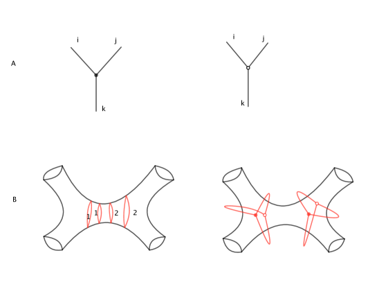
Figure 3: Here we give some examples for line operator of $A_{2}$ theory on a fourth punctured sphere. Left: Wilson line with representation $R=2w_{1}+2w_{2}$ which is represented by colored closed curve. Right: A web operator formed by junctions.

2.2 Tropical label for line operators and OPE

We can label the line operator from colored A lamination by irreducible representation of $su(N)$ lie algebra, but we do not have a good label for line operator from webs. There is a tropical label which is applicable to all the line operators considered above. Here we simply review the basic concepts and the interested reader can find more details in [9, 11, 17].

These tropical labels are defined by using a triangulation of $\Sigma$ and define a quiver [25, 21], and the total number of quiver nodes are

$$r=2n_{r}+n_{f},$$ (2)

where $n_{r}$ is the number of Coulomb branch dimensions of the field theory and $n_{f}$ is the number of mass parameters. Tropical $a$ coordinates are simply a set of discrete numbers defined on the quiver nodes. For a line operator in fundamental (defining) representation $w_{1}$, one could find its tropical $a$ coordinates by calculating the trace of its monodromy around the closed curve using the rule found in [26].

To do the calculation explicitly, we need to choose a orientation of Riemann surface, which will induce an orientation on the closed curves, and we take the line operator wrapping once along this oriented closed curve as the line operator in $w_{1}$. This is the rule used in [11]. The other colored closed curves have the same orientation as $w_{1}$. We have the following equivalence relation about the orientation and label: changing the orientation of the closed curve and change the label from $i\rightarrow N-i$ would denote a same line operator, and using this rule, we can replace all the colored closed curves by oriented curves with label less than $[N/2]$. In the $A_{2}$ case, we can use the above equivalence to replace the colored closed curves with oriented curves without any label. The above rule also induces an orientation on junctions: the orientation of black junction is coming out, while the orientation of white junction is coming in. Again, we can change the orientation and label simultaneously to put all the labels of the leg to be less than $[N/2]$.

The result from monodromy calculation is always a positive Laurent polynomial in cluster $X$ coordinates, which is denoted as $I(L)$ and called canonical map. This canonical map simply means that we represent a line operator by a Laurent polynomial! The tropical $a$ coordinate is simply the exponent of the leading order term, which is a set of positive integers with fraction ${1\over N}$. For the details on the calculation and examples, see [11].

Using the canonical map, one can calculate OPE of two line operators by simply multiplying two Laurent polynomials, and OPE has the following familiar form:

$$I(L_{1})I(L_{2})=\sum_{L}C_{L_{1}L_{2}}^{L}I(L),$$ (3)

here $C_{L_{1}L_{2}}^{L}$ is a positive integer. The leading order term has tropical $a$ coordinates $a(L_{1})+a(L_{2})$, and the coefficient $C_{L_{1}L_{2}}^{L_{1}+L_{2}}=1$. In fact, the web structure reviewed in last subsection is found by calculating the OPE explicitly.

Instead of using canonical map, OPE can also be calculated using remarkably simple skein relations [11], see figure. 4 for several simple examples. The procedure of finding OPE geometrically is following: first draw two line operators which will intersect each other, and then use skein relation to resolve the intersection. See figure. 5 for an example.

Figure 4: Skein relations which can be used to find OPE in a simple way. Here we only show some simple examples without showing the full set of skein relations.

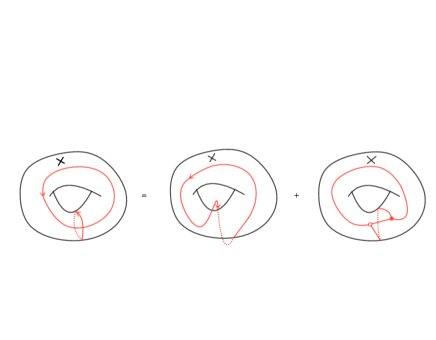
Figure 5: The use of skein relation in finding OPE of line operators of $A_{2}$ theory on a once punctured torus.

3 Gauge theory interpretation and duality action on line operators

In this section, we will identify the geometric representation of the familiar Wilson-’t Hooft line operators in field theory and study the duality actions on them. We only consider theory defined Riemann surface with regular punctures, and use the un-oriented picture of line operators.

3.1 Classification of Wilson-’t Hooft line operators from field theory

It is shown by Kapustin [19] that a general Wilson-’t Hooft line operator of $\mathcal{N}=4$ SYM is classified by a pair of weights modulo the action of Weyl group:

$$(B,\mu)/W,$$ (4)

here $B$ is a magnetic weight of dual group $G^{L}$ and $\mu$ is an electric weight of $G$. For pure electric line operator, the classification is equivalent to the classification of irreducible representation $G$, and similarly pure magnetic line operator is also equivalent to an irreducible representation of $G^{L}$. When $B$ and $\mu$ both nonzero, we can first use Weyl group to fix $B$ to be highest weight of an irreducible representation. Let’s denote the highest weight of fundamental representations of $su(N)$ as $\omega_{i}$, then the highest weight of an irreducible representation of $su(N)$ can be written as

$$B=\sum m_{i}\omega_{i},$$ (5)

with $m_{i}\geq 0$. After fixing the magnetic weight, the electric weight can take arbitrary values

$$\mu=\sum n_{i}\omega_{i},$$ (6)

and $n_{i}$ can take both positive and negative values. Here we ignore the constraints on $m_{i}$ and $n_{i}$ due to the global form of the gauge group.

In our case, there are also fundamental matter and sometimes the dual gauge group is also $G$. Therefore we claim the most general Wilson-’t Hooft line operators for a duality frame with $n$ gauge groups are classified by

$$(B_{1},B_{2},\ldots,B_{n},\mu_{1},\mu_{2},\ldots,\mu_{n})/W,$$ (7)

and $B_{i}$ and $\mu_{i}$ can be expanded using the fundamental weights, and again using Weyl transformation we can take $B_{i}$ to be a highest weight. The coefficients are constrained by several mutual locality conditions: a: the line operator should be mutually local with the matter content. b: the line operator should be mutually local with each other. These issues will be discussed later, as the results in this section are not affected by these issues.

3.2 Geometric representation

Let’s now come back to our geometric representation of line operator, and we will identify the geometric object with the line operator from field theory classification. To find this identification, we need to take a pants decomposition which represents a weakly coupled duality frame of field theory. Let’s denote our punctured Riemann surface as $\Sigma_{g,n}$, and fix a pants decomposition: there are $2g-2+n$ pair of pants representing $T_{N}$ theory, and $3g-3+n$ $SU(N)$ gauge groups represented by simple closed curves $C_{i}$. It is now easy to find the Wilson loop of gauge group $G_{i}$ associated with $C_{i}$: they are represented by a set of closed curves around $C_{i}$, and it is shown in section 2 that this type of line operator is indeed classified by the irreducible representation of $su(N)$. Similarly, by considering the line operators supported on dual cycle of $C_{i}$, we find that the magnetic line operators are also classified with irreducible representation of $su(N)$.

For more general line operator, we need to introduce Dehn-Thurston coordinates for unoriented closed curves (colors will be introduced later). Given a pants decomposition, the Dehn-Thurston coordinates for a multiple curve $l$ are a set of integers

$$(m_{1},m_{2},\ldots,m_{3g-3+n},t_{1},t_{2},\ldots,t_{n}).$$ (8)

Here $m_{i}$ is the geometric intersection number of $l$ and $C_{i}$, and $t_{i}$ is the twisting number along the annulus region around $C_{i}$. $m_{i}$ is positive, and $t_{i}$ can be positive or negative based on its winding direction (if $m_{i}=0$, then $t_{i}\geq 0$), see figure. 6. Dehn-Thurston coordinates in a pants satisfy the following condition

$$m_{i}+m_{j}+m_{k}\in\text{even}$$ (9)

if $i,j,k$ are in same pants.

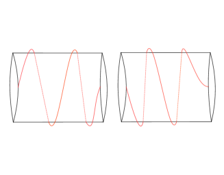
Figure 6: Left: the twisting parameter is positive. Right: the twisting parameter is negative.

On the other hand, given a set of Dehn-Thurston coordinates satisfying the above condition, we can reconstruct the multiple curves. The curves on the pants is constructed using basic building block represented by simple curves $l_{12},l_{13},l_{23},l_{11},l_{22},l_{33}$, here $l_{ij}$ denote the curves connecting $i$th and $j$th boundary, and $l_{ii}$ are the open curves connecting the same boundary. The number of these curves are determined by the coordinates $m_{i}$ and we have

$$2l_{ii}=max(m_{i}-m_{j}-m_{k},0)$$

$$2l_{ij}=max(m_{i}+m_{j}-m_{k},0)-l_{ii}-l_{jj}$$

There are actually four cases based on the relative values of $m_{i}$, and see figure. 7 for an illustration. The construction of of the curves for twisting parameter $t_{i}$ is simple, see figure. 8: we use $m_{i}$ horizontal curves on the tube and use $t_{i}$ loops around the circle, then we use skein relation of $A_{1}$ theory to resolve the intersections. There are two options in using Skein relations, and the rule is to use one option for all the intersections. This gives the positive and negative windings respectively, see figure. 8.

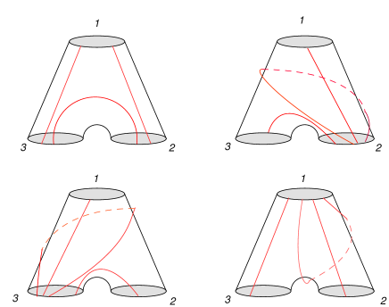
Figure 7: Curve models based on different choices of magnetic coordinates on a pants.

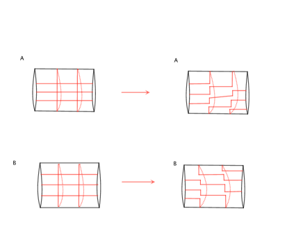
Figure 8: One can find the curves from twisting parameter by resolving the intersections in a certain direction which is determined by the sign of twist parameters.

Now let’s consider colored A lamination, namely we consider multiple curves with labels, then the Dehn-Thurston coordinates are further partitioned according to the colors. Consider a single closed curve $c_{i}$ in the pants decomposition, and assume the partition from the colors are

$$(m_{1i},m_{2i},\ldots,m_{N-1i},t_{1i},t_{2i},\ldots,t_{N-1i})$$ (11)

It is natural to identify this line operator as the Wilson-’t Hooft line operator with label $(B,\mu)$:

$$B_{i}=m_{1i}w_{1}+m_{2i}w_{2}+\ldots+m_{N-1i}w_{N-1},~{}~{}~{}~{}\mu_{i}=t_{1i}w_{1}+t_{2i}w_{2}+\ldots+t_{N-1i}w_{N-1}$$ (12)

Notice that all the electric coordinates have the same sign.

Obviously line operators from colored A lamination do not exhaust the whole set of line operators derived from field theory. The question is: What is the geometric representation for other line operators? The answer is that they are represented by webs. To see this, let’s consider a theory defined by $A_{2}$ theory on a once punctured torus. Let’s take a weakly coupled duality frame by choosing a pants decomposition of once punctured torus, and let’s simply take the closed circle $a$ as the one defining the weakly coupled gauge group. Wilson loops are represented by closed curves around $a$ cycle, and ’t Hooft loops are represented by closed curves around $b$ cycle.

Let’s now consider the OPE between the Wilson loops $W_{0,\omega_{1}}$, $W_{0,\omega_{2}}$ and ’t Hooft line operator $T_{\omega_{1},0}$, $T_{\omega_{2},0}$. One can use skein relation to find the detailed OPE, see figure. 9, and we find some line operators represented by the webs. It is natural to expect that those webs representing various Wilson-’t Hooft line operators, see figure. 9, and one can find all the missing line operators. It is not difficult to identify all the Wilson-’t Hooft line operators using our OPE construction [31]. For our consideration of duality action, it is enough to consider line operators from colored A laminations.

One thing we want to stress is that there are new line operators besides the ordinary Wilson-’t Hooft line operators associated with gauge group, see figure. 10. These new line operators can be interpreted as the line operators of $T_{N}$ theory, and they have rather important applications to the construction of Hamiltonian of the underlying integrable system [31].

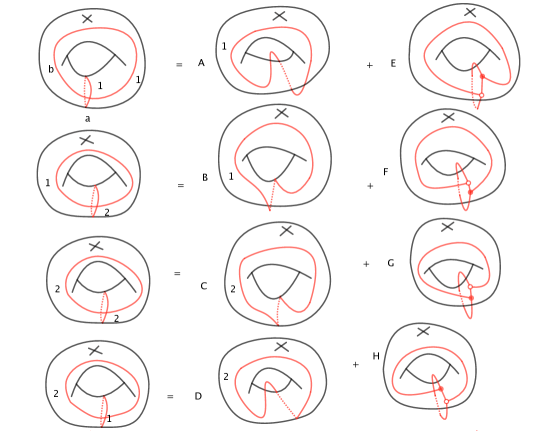
Figure 9: Various Wilson-’t Hooft line operators can be found by doing OPE between Wilson and ’t Hooft line operators: A: $\text{WL}_{w_{1},w_{1}}$, B: $\text{WL}_{w_{1},-w_{1}}$, C: $\text{WL}_{w_{2},w_{2}}$, D: $\text{WL}_{w_{2},-w_{2}}$. E: $\text{WL}_{w_{1},-w_{2}}$; F:$\text{WL}_{w_{1},w_{2}}$; G: $\text{WL}_{w_{2},w_{1}}$; H: $\text{WL}_{w_{2},-w_{1}}$

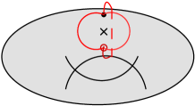
Figure 10: New line operator which is not included in Wilson-’t Hooft line operators.

3.3 Duality action on line operators

The duality group of four dimensional gauge theory is identified with the mapping class group of the underlying Riemann surface, which is generated by the Dehn twist. The Dehn twist around a closed curve acts on line operator coming across that line operator as from colored A lamination in certain class at circle $i$ as:

$$(m_{i}^{{}^{\prime}},t_{i}^{{}^{\prime}})=(m_{j},t_{i}\pm m_{i})$$ (13)

See figure. 11. This action can be thought of as shifting the $\theta$ angle of gauge group by $2\pi$, and the change of electric charge due to the $\theta$ angle is essentially the Witten effect [32]. The generalization of this formula to line operators represented by colored A lamination with label $i$ is simple: for a line operator with label around circle $i$

$$B_{i}=m_{1i}w_{1}+m_{2i}w_{2}+\ldots+m_{N-1i}w_{N-1},~{}~{}~{}~{}\mu_{i}=t_{1i}w_{1}+t_{2i}w_{2}+\ldots+t_{N-1i}w_{N-1}$$

$$B_{i}^{{}^{\prime}}=m_{1i}w_{1}+m_{2i}w_{2}+\ldots+m_{N-1i}w_{N-1},~{}~{}~{}$$

$$\mu_{i}^{{}^{\prime}}=[t_{1i}+\pm m_{1i}]w_{1}+[t_{2i}\pm m_{2i}]w_{2}+\ldots+[t_{N-1i}\pm m_{N-1i}]w_{N-1}$$ (14)

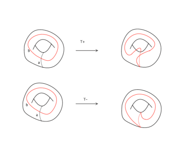
Figure 11: Action of $T$ transformation on line operators.

Now let’s fix a pants decomposition, and study the transformation of the Dehn-Thurston coordinates in changing the Pants decomposition. It is proven in [33] that pants decompositions are related by two fundamental moves: one is the S-move on once punctured torus, and the other one is the A move on fourth punctured sphere, see figure. 12. These two moves are actually the S duality action on the corresponding gauge group.

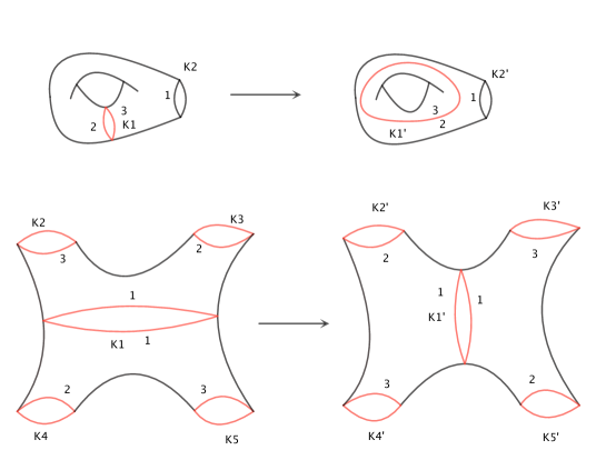
Figure 12: Two elementary moves relating pants decomposition. Top: S move relating two pants decomposition of a once punctured torus. Bottom: A move relating two pants decomposition of a fourth punctured sphere

The transformation rule on Dehn-Thurston coordinates are found by Penner [10]. Since there is only one pants, we have $m_{2}=m_{3}$ and $r=\lambda_{12}=\lambda_{13}$. The formula for the S-move on coordinates reads

$$\lambda_{11}^{{}^{\prime}}=max(r-|t_{1}|,0)$$

$$\lambda^{{}^{\prime}}_{12}=\lambda^{{}^{\prime}}_{13}=L+\lambda_{11},$$

$$\lambda_{23}^{{}^{\prime}}=|t_{1}|-L$$

$$t_{2}^{{}^{\prime}}=t_{2}+\lambda_{11}+max(min(L,t_{1}),0)$$

$$t_{1}^{{}^{\prime}}=-sgn(t_{1})(\lambda_{23}+L)$$ (15)

here $L=r-\lambda_{11}^{{}^{\prime}}$. From the above formula, we can easily find the new magnetic coordinates associated with the pants.

For one application, let’s consider line operator with $m_{1}=0$, and we have $m_{2}=m_{3}=m$, and $\lambda_{11}=\lambda_{13}=\lambda_{12}=0,~{}L=0$, so we can focus locally on a line operator labeled by coordinates $(m,t)$, and the above formula becomes

$$\lambda_{23}^{{}^{\prime}}=m^{{}^{\prime}}=|t_{1}|$$

$$t_{1}^{{}^{\prime}}=-sgn(t_{1})m$$ (16)

The generalization of above formula to line operators of higher rank theory is following

$$m_{1i}^{{}^{\prime}}=|t_{1i}|,~{}~{}m_{2i}^{{}^{\prime}}=|t_{1i}|,~{}~{}\ldots,~{}~{}m_{Ni}^{{}^{\prime}}=|t_{N-1i}|$$

$$t_{1i}^{{}^{\prime}}=-sgn(t_{1i})m_{1i},~{}~{}t_{2i}^{{}^{\prime}}=-sgn(t_{2i})m_{2i},~{}~{}\ldots,~{}~{}t_{N-1i}^{{}^{\prime}}=-sgn(t_{N-1i})m_{N-1i},$$ (17)

This formula is derived by only considering the closed curves with the same label, and apply the above formula. The result is the same as found in [19]. The transformation rule for the $A$ move is much more complicated, see [10] for the detailed formula. The generalization to the higher rank theory is straightforward by considering one type of colored closed curve at one time.

4 Dirac paring and mutual locality condition

We used the closure of OPE condition to find the web structure of line operator of class ${\cal S}$ theory. In this section, we define Dirac product and mutual locality conditions between line operators, and we use the oriented picture for line operators.

The definition of Dirac product is the following: there is a natural Poisson structure on the space of line operators:

$$\{L_{1},L_{2}\}=AI_{1}+\ldots$$ (18)

and here $I_{1}$ is the leading order line operator in the OPE of $L_{1}$ and $L_{2}$. We define coefficient $a$ as the Dirac product between two line operators as

$$<L_{1},L_{2}>=A,$$ (19)

and this product is antisymmetric in exchanging $L_{1}$ and $L_{2}$. Knowing the explicit tropical coordinates of $L_{1},L_{2}$, the constant $A$ has an extremely simple form

$$A=\sum\epsilon_{ij}a_{1i}a_{2j}=-\sum x_{1i}a_{2i}$$ (20)

where $x_{1i}$ is the tropical $x$ coordinates of the line operator $L_{1}$. Two line operators are mutually local if the Dirac product between them are integers:

$$<L_{1},L_{2}>\in Z.$$ (21)

The reason this is called mutual locality condition is that this ensures line operator is not going to pick up a non-trivial phase in going around other line operators. There are several useful facts about the Dirac product we defined:

• In defining tropical $a$ coordinates, we need to choose a coordinate system defined by a quiver on Riemann surface. However, it is easy to prove that locality condition is independent of coordinate systems, see appendix for a simple proof.

• If $L$ is mutually local with a set of line operators $L_{i}$, then $L_{1}$ is mutually local with any line operators formed by doing OPE of $L_{i}$. The reason is the following: consider the OPE of $L_{i}$

  $$\prod L_{j}^{n_{j}}=I_{1}+C_{2}I_{2}+\ldots,$$ (22)

  here $I_{1}$ is the leading order term in OPE whose $a$ coordinates are simply the sum of $\sum n_{i}L_{i}$, and $I_{2}$ is the sub-leading order term and $C_{2}$ is the OPE coefficient. According to our definition, we have

  $$<L,I_{1}>=\sum n_{j}<L,L_{j}>,$$ (23)

  Since $<L,L_{j}>$ is integer, we see that $<L,I_{1}>$ is also a integer. Moreover, the difference of tropical $a$ coordinates of $I_{i}$ and $I_{1}$ is integer, and $<L,I_{j}>$ is also a integer for any $j$, so $L$ is mutually local with all the line operators found by doing OPE between $L_{i}$.

Because of the second fact, we only need to study the mutual locality condition on colored closed curves, and consider only web operators from doing OPE of mutually local line operators from colored closed curves.

For our application, there is actually a simple graphical rule. Let’s take an orientation of Riemann surface and calculate the Poisson bracket of two line operators with label $1$, and explicit calculations shows that

$$L_{1}\cdot L_{2}={ij/N},~{}~{}~{}~{}\text{or}~{}~{}~{}~{}L_{1}\cdot L_{2}={-ij/N}$$ (24)

The sign depends on the orientation, see figure. 13. The Dirac product of two general line operators are found by counting the signed intersection number between two set of closed curves. For later convenience, we multiply Dirac product of two line operators by $N$, and define the mutual locality condition as follows

$$L_{1}\cdot L_{2}\in pN,$$ (25)

here $p$ is a integer.

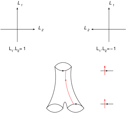
Figure 13: Up: Dirac paring for two oriented curves with label $1$. Bottom: a closed curve has opposite contributions to Dirac pairing at two intersections with the boundary of the pants.

Now here comes the crucial point: the above geometric observation of Dirac product tells us that the mutual locality condition depends on signed intersection number (or algebraic intersection number) of oriented closed curves, and algebraic intersection number is naturally defined on homology class instead of homotopy class. In studying mutual locality condition, we should work on homology theory instead of homotopy theory in determining the locality between the line operators, which makes the task much easier, as the homology theory is abelianization of the homotopy theory. When we talk about mutual locality condition between line operators, we actually mean the corresponding homology class, and each homology class consists many distinct line operators!

It is easy to find the corresponding homology class of a line operator $L$ represented by oriented colored closed curve. We first choose a basis of homology group and find the corresponding homology class of each oriented closed curve as $[c_{j}]$, then the corresponding homology class of $L$ is simply

$$[L]=\sum_{j}i[c_{j}],$$ (26)

where $i$ is the color of $c_{j}$.

Now let’s consider mutual locality condition between line operators and matter represented by three punctured sphere. We define the Dirac pairing as the Dirac product between the the oriented line operators and the oriented boundary circles of a pant. Now each curve in the pants has a positive and negative contribution to the Dirac product, so their contributions cancel, and the locality condition is always obeyed for the line operator from closed curves, see figure. 13. In $A_{1}$ case, it is verified in [8] that all possible line operators mutually local with the matter are represented by closed curves. It is interesting to verify that all possible Wilson-’t Hooft line operators mutually local with the matter can be represented by the line operator considered in last section.

5 Allowed set of line operators and discrete $\theta$ angle

Typically, a gauge theory is defined by first specifying the gauge group $G$, and the allowed matter coupled to gauge group is constrained to transform in representation of $G$. After specifying the gauge theory, we would like to ask what is the possible choice of line operators. The allowed set of line operators are determined as follows (for zero $\theta$ angles):

• Given the gauge group $G$, the Wilson (electric) line operator is classified by irreducible representation of $G$.

• The allowed set of ’t Hooft (magnetic) line operators is found by imposing the locality condition with matter and Wilson line operators.

• The allowed set of dyonic line operators is determined by imposing locality condition with electric, magnetic line operators and matter.

We need to include all possible line operators consistent with above conditions. There are new possibilities by turning on discrete $\theta$ angles, and the set of line operators are found by doing $T$ transformation on the above set of line operators. So the choice of line operators is not uniquely fixed by gauge group $G$ and matter content, we need to specify discrete $\theta$ angles.

We would like to generalize the above classification of line operators to class ${\cal S}$ theories defined on a genus $g$ Riemann surface with $n$ punctures. In our case, given a duality frame corresponding to a pants decomposition, the lie algebra of the gauge group is fixed as $g=su(N)^{3g-3+n}$ and the matter content is just $(2g-2+n)$ $T_{N}$ theory. We would like to classify the allowed set of line operators by imposing following four conditions:

• The line operators are mutually local with the matter content.

• The line operators form a closed set in doing OPE.

• The line operators satisfy the mutual locality condition.

• The sets of line operators form a maximal set, i.e. they are not a subset of any other allowed choice.

The first condition implies the identification of line operator (generators) with the colored closed curves on Riemann surface. The second condition has been used in [11] to find new line operators represented by webs. We would like to impose third and fourth conditions on line operators using the mutual locality conditions defined in last section.

Since web operators are found by doing OPE of operators from colored closed curves, and they will be mutually local to each other if the corresponding colored line operators are mutually local, we only need to impose condition on colored closed curve. Moreover, the mutual locality condition is a condition on homology class and not the homotopy class, so the task of classification is much easier. In the following we always talk about the homology class, and it should be clear that there are many distinct line operators in a single homology class.

5.1 Gauge group from choice of Wilson line operators

Usually we first know the gauge group $G$ and matter content, then we try to find the allowed line operators. Here for the class ${\cal S}$ theory, the situation is reversed. We only know the lie algebra, and we want to find the gauge group from allowed set of line operators.

Let’s choose a pants decomposition of oriented Riemann surface and focus on a gauge group represented by a closed circle $c_{i}$ whose homology class is denoted $[c_{i}]$. The global form of gauge groups can be found by the allowed homology class of line operators supported on $[c_{i}]$:

• If $[c_{i}]$ is in trivial homology class or more generally its intersection number with other homology class is zero, then the gauge group is $SU(N)$ as line operators in homology class $[c_{i}]$ is mutually local with all the other line operators, in particular, Wilson loop in defining representation of $su(N)$ is allowed and therefore the gauge group has to be $SU(N)$.

• If $[c_{i}]$ is in a non-trivial homology class, and the minimal allowed homology class is $k[c_{i}]$ and all the other allowed ones are integer multiple of the minimal one, notice that $k$ has to be divided by $N$ (otherwise the choice of line operators are not closed under OPE). Then the gauge group is $SU(N)/Z_{k}$.

However, we can not choose the minimal homology classes arbitrarily. To illustrate this point, let’s consider a pants whose three flavor symmetries are gauged, and we assume that three homology class associated with boundaries are non-trivial, see figure. 14. Let’s assume that the minimal choice of homology class around $[a_{1}]$ and $[a_{2}]$ are ($k_{1}[a_{1}]$, $k_{2}[a_{2}]$), then the choice of homology class around $[a_{3}]$ is fixed, since we have the following relation between homology class:

$$[a_{3}]=-[a_{1}]-[a_{2}],$$ (27)

and we can find line operators in integer multiple of $[a_{3}]$ homology class using OPE. It is easy to find what is the minimal homology class of $[a_{3}]$: let’s denote the minimal homology class around $[a_{3}]$ as $p[a_{3}]$, and $p$ can be found by imposing the condition:

$$nk_{1}[a_{1}]+mk_{2}[a_{2}]=p[a_{3}]\rightarrow nk_{1}[a_{1}]+mk_{2}[a_{2}]=-p[a_{1}]-p[a_{2}],$$ (28)

which implies that $p$ is the minimal number such that

$$nk_{1}=p,~{}~{}~{}mk_{2}=p;$$ (29)

and $p$ is uniquely fixed once $k_{1}$ and $k_{2}$ is given. The gauge group associated with $[a_{3}]$ is $SU(N)/Z_{p}$.

Figure 14: The gauge group from choice of Wilson loops on three boundaries of a trinion.

The above consideration only tells us the local (a single gauge group) form of the gauge group, to find out the real form of the gauge group, we need to use the matter content which is described by $T_{N}$ theory.

$T_{N}$ theory is defined by compactifying 6d theory on a sphere with three full punctures, and the lie algebra of flavor symmetry is

$$su(N)_{a}\times su(N)_{b}\times su(N)_{c},$$ (30)

and naively the center would be $\Gamma=Z_{N}^{a}\times Z_{N}^{b}\times Z_{N}^{c}$, however, as pointed out in [18], the true center is actually not $\Gamma$ but just a single $Z_{N}$. Assuming the generator of $Z_{N}^{a},Z_{N}^{b},Z_{N}^{c}$ as $\gamma_{1},\gamma_{2},\gamma_{3}$, then the above statement of a single $Z_{N}$ center of $T_{N}$ theory can be interpreted as relations between the three generators:

$$\gamma_{1}\gamma_{2}^{-1}=1,~{}~{}~{}~{}~{}\gamma_{2}\gamma_{3}^{-1}=1.$$ (31)

$T_{N}$ theory has a set of operators $Q_{abc}$ which transforms as trifundamental representation of the flavor group, and therefore is not invariant under the center $Z_{N}$. This puts constraints on possible global form of gauge group: $Q_{abc}$ should be invariant under ungauged center of the flavor group. If only one flavor group is gauged, then the gauge group has to be $SU(N)$, and if only two flavor groups are gauged, then the gauge group has to be $SU(N)/(Z_{k})_{1}\times SU(N)/(Z_{k})_{2}$, and the generators of $(Z_{k})_{1}$ and $(Z_{k})_{2}$ are $\gamma_{1}^{N/k}$ and $\gamma_{2}^{-N/k}$. Due to relation [31], $T_{N}$ theory is invariant under the ungauged center. In general, if three flavor groups of $T_{N}$ theory are gauged, and we have following choices :

• the gauge group is $SU(N)\times SU(N)\times SU(N)$: $Z_{N}$ is gauged, and there is no residual discrete flavor symmetry.

• the gauge group is $SU(N)/Z_{k}\times SU(N)/Z_{k}\times SU(N)$, and the generators of two $Z_{k}$ are $\gamma_{1}^{N/k}$ and $\gamma_{2}^{-N/k}$.

• the gauge group is $SU(N)/Z_{k}\times SU(N)/Z_{k}\times SU(N)/Z_{k}$. The generators for three ungauged center are $(\gamma_{1}^{N/k_{1}},\gamma_{2}^{-N/k_{1}},\gamma_{3}^{N/k_{1}})$.

• the gauge group is $SU(N)/Z_{k_{1}}\times SU(N)/Z_{k_{2}}\times SU(N)/Z_{k_{3}}$. To ensure $T_{N}$ theory invariant under the ungauged center, one can not choose $k_{i}$ arbitrarily. Let’s assume that we fix $k_{1}$ and $k_{2}$ with $k_{1}\neq k_{2}$, and $k_{1}$ and $k_{2}$ should be divided by N. The generators for first two ungauged center are $(\gamma_{1}^{N/k_{1}},\gamma_{2}^{-N/k_{2}})$. Using relation [31], this two center generate a group $Z_{p}$ whose generators is $\gamma_{2}^{N/p}$. $p$ is determined by finding the minimal $p$ such that

  $$nk_{1}=p,~{}~{}~{}mk_{2}=p;$$ (32)

  Here $n$ and $m$ are integers. To make sure $T_{N}$ theory invariant under the ungauged center, we must have

  $$k_{3}=p,$$ (33)

  and the third gauge group has to be $SU(N)/Z_{p}$. This constraint is precisely the one we found using the homology class of pants!

5.2 Action of $T$ and $S$ transformation on homology class

We can use S and T transformation to relate different gauge theories. S duality is simply interpreted as changing the pants decompositions which could be decomposed into two fundamental moves; $T$ transformation corresponds to doing Dehn twist around closed circle whose homology class is denoted as $[a]$, and the action of Dehn twist on homology class $[b]$ is [34]:

$$T_{a}([b])=[b]+\hat{i}(a,b)[a],$$ (34)

and here $\hat{i}(a,b)$ is the algebraic intersection number between two homology classes, which only depends on homology class $[a]$ and $[b]$. Physically, $T$ transformation corresponds to change the discrete $\theta$ angle by $2\pi$.

The $S$ duality action on homology class is more complicated. Consider once punctured torus and the $S$ move, $S$ duality action simply exchanges $[a]$ and $[b]$ cycle. Now to preserve the canonical intersection number, the action is actually

$$[a^{{}^{\prime}}]=[b],~{}~{}~{}[b^{{}^{\prime}}]=-[a]$$ (35)

so the $S$ duality action on a general homology class $[l]=n[a]+m[b]+\ldots$ is

$$S[l]=m[a^{{}^{\prime}}]-n[b^{{}^{\prime}}]+\ldots.$$ (36)

One can also find $S$ duality action on homology class associated with the $A$ move on fourth punctured sphere, for our purpose, the action simply exchanges the cycle associated with the original gauge group and the cycle associated with the dual cycle.

5.3 Examples

After connecting all the basic tools, we will give various examples in this section on the choice of allowed line operator, and then identify the global form of the gauge groups and discrete $\theta$ angles. Duality webs among these theories are also studied.

5.3.1 $T_{N}$ theory: no choice

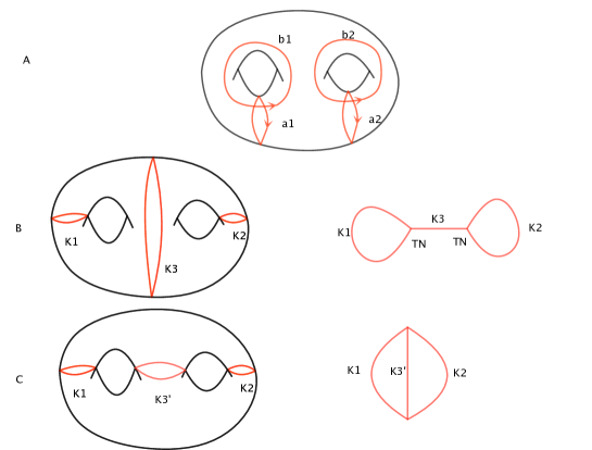
Figure 21: Basis of homology class of genus two Riemann surface

Let’s discuss first the allowed set of line operators of $T_{N}$ theory. The basic non-trivial line operators of $T_{N}$ theory are formed by webs built from two three junctions, see figure. 21. Any two web operators are mutually local, as the two intersections have opposite orientation, and they are mutually local, see figure. 21. Therefore, there is no choice of line operators for $T_{N}$ theory, which agrees with the conclusion in [18].

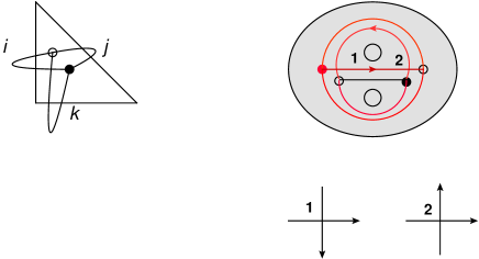
Figure 15: Left: the generators for non-trivial line operators of $T_{N}$ theory. Right: the intersections between two web operators; Two intersections have opposite intersection number, so two line operators are mutually local.

5.3.2 Sphere with punctures: no choice

The generators for the homology group of punctured sphere are shown in figure. 16, and they satisfy the condition:

$$\gamma_{1}\gamma_{2}\ldots\gamma_{n}=1.$$ (37)

Figure 16: The generators of homology class of a punctured sphere.

The algebraic intersection number of these generators are zero, therefore the mutual locality condition is always satisfied for any line operators. Due to the maximality condition on the choice of line operators, we can not choose a subset, therefore there is a unique choice of line operators associated with the sphere: all possible line operators considered in [11] should be included. When we choose a duality frame, i.e. take a pants decomposition, then the gauge groups are $SU(N)$ as basic Wilson line associated with the defining representation of $SU(N)$ is allowed.

5.3.3 Genus one case

Let’s first consider $\mathcal{N}=2$ theory defined by a torus with one regular singularity. The classification of line operators is the same as the $\mathcal{N}=4$ theory discussed in [20], here we show how that classification can be implemented using our geometric picture (our consideration is also applied to $\mathcal{N}=4$ case).

The non-trivial homology class of torus is generated by two cycles $a$, $b$, and $c$ around the puncture , and the intersection number is given by

$$[a]\cdot[b]=1.$$ (38)

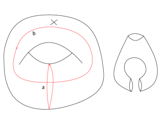
Figure 17: Left: the homology class of a once punctured torus. Right: one pants decomposition of once punctured torus.

see figure 17. $c$ has zero intersection numbers with other two generators, so it can not give any constraints from the consideration of mutual locality condition, and we can ignore it from now on. Let’s take one weakly duality frame which is described by the pants decomposition of the torus, which is defined by a closed curve whose homology class can be taken as $[a]$.

Let’s start with zero $\theta$ angle, and the allowed set of line operators are classified as:

• The minimal Wilson loop is chosen in homology class $k[a]$ with $k$ divides N, i.e. $kk^{{}^{\prime}}=N$. This implies that the gauge group is $SU(N)/Z_{k}$. The choice of electric line operators are $n[a]$ with

  $$n=p_{1}k.$$ (39)

• The pure magnetic line operators are chosen by imposing the mutual locality condition with electric line operators. Let’s denote the corresponding homology class as $m[b]$, and we have

  $$m[b].k[a]=p_{2}N\rightarrow m=p_{2}k^{{}^{\prime}},$$ (40)

• Let’s denote the homology class of a general line operator as $n[a]+m[b]$, we require it to be mutually local with the basic electric and magnetic line operators:

  $$(n[a]+m[b])\cdot k[a]=p_{2}N,~{}~{}~{}(n[a]+m[b])\cdot k^{{}^{\prime}}[b]=p_{1}N$$ (41)

  which implies that $m=p_{2}k^{{}^{\prime}}$ and $n=p_{1}k$.

It is easy to check the mixed line operators determined by above conditions are mutually local to each other. In summary, the homology class of allowed line operators are

$$p_{1}k[a]+p_{2}k^{{}^{\prime}}[b],$$ (42)

We can represent the choice of line operators by a lattice in which $x$ ($y$) coordinates are coefficient of $[a]$ ($[b]$), see figure. 18. In fact, it is sufficient to just look at the lattice inside the fundamental square bounded by four points $(0,0),(0,N),(N,0),(N,N)$. The theory defined by above data is denoted as $(SU(N)/Z_{k})_{0}$. This type of lattice is essentially the same as the one given in [20], here we interpret them as the allowed homology class of line operators.

Figure 18: Homology class of allowed line operators.

We can find other theories by doing $T$ transformation (turning on discrete $\theta$ angle) around $a$. Let’s start with $SU(N)/Z_{k}$ gauge theory with zero $\theta$ angle, and do $T$ transformation which corresponds to one Dehn twist around circle $a$. For a line operator in homology class $[l]=p_{1}k[a]+p_{2}k^{{}^{\prime}}[b]$, the intersection number with $[a]$ is $[a]\cdot[l]=p_{2}k^{{}^{\prime}}$, and using the formula [34], the action of Dehn twist $T_{+}^{n}$ on homology class $[l]$ is

$$p_{1}k[a]+p_{2}k^{{}^{\prime}}[b]\rightarrow({p_{1}k+np_{2}k^{{}^{\prime}}})[a]+p_{2}k^{{}^{\prime}}[b];$$ (43)

Using this formula, we see that the choice of Wilson loop is not changed, but the choice of magnetic and mixed line operator is changed, which will give new theories if

$$np_{2}k^{{}^{\prime}}\neq kp.$$ (44)

for any $p_{2}$. We label these new theories as $(SU(N)/Z_{k})_{n}$ with $n$ means the theory is derived by doing $n$ Dehn twist for the theory with zero $\theta$ angle. See figure. 18 for some examples, and it is easy to find all possible lattices from doing $T$ transformation on theory with zero $\theta$ angle. There are some simple features about the $T$ transformation by looking at the above formula:

• If the gauge group is $SU(N)$ which means that the electric homology class is taking all possible integers, then the $T$ transformation will not change the charge lattice.

• If the gauge group is $SU(N)/Z_{k}$, then the maximal number of non-trivial Dehn-twist is $(k-1)$.

• $T$ transformation preserves the mutual locality condition: if two line operators are mutually local before the transformation, they will be mutually local after the transformation.

So we get an allowed set of line operators satisfying our four conditions after $T$ transformation due to the third feature.

To identify the dual gauge theory after $S$ transformation, we need to look at the action of $S$ transformation on homology class:

$$n[a]+m[b]\rightarrow m[a^{{}^{\prime}}]-n[b^{{}^{\prime}}]$$ (45)

The action on charge lattice is simple: the new fundamental region is found by rotating 90 degree of the fundamental region in clockwise direction.

Using the above $S$ and $T$ transformation on charge lattice, it is then easy to identify the dual theories. There are very interesting duality webs as studied in [20]. Notice that not all theories can be related by $S$ and $T$ transformations, and there are interesting orbit structure. We only give several simple examples here, the interested reader can work out more complicated example using our geometric representation.

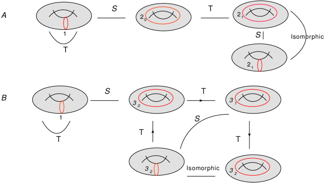
Figure 19: Allowed homology class of line operators.

Torus with two punctures:

The homology group of this geometry is generated by $a$ cycle and $b$ cycle of the torus, and two closed cycles around the punctures. The only nontrivial intersection forms among the generators are

$$[a]\cdot[b]=1.$$ (46)

The classification of the allowed line operators is the same as the above one. Here we want to study the gauge theory interpretation and point out one new novelty.

There are two duality frames of this theory: one duality frame has one gauge group coupled to a single $T_{N}$ theory, and the other gauge group coupled to two $T_{N}$ theories. In one duality frame shown in figure. 20A, we can choose the minimal homology class as $k[a]$, and therefore the gauge group $G_{1}=SU(N)/Z_{k}$. The closed curve associated with $G_{2}$ is in trivial homology class, and therefore the gauge group is $G_{2}=SU(N)$. The action of $T$ and $S$ duality on $G_{1}$ group is the same as above case, and we do not repeat the analysis here.

What is interesting is the $S$ and $T$ transformation on gauge group $G_{2}$. First of all, $T$ transformation would not change the allowed set of line operators. After doing $S$ transformation on group $G_{2}$, we went to duality frame shown in figure. 20B. Now the closed curve associated with $G_{2}^{{}^{\prime}}$ is not in trivial homology class, and it is actually in homology class $[a]+[\Gamma_{1}]$, since $\Gamma_{1}$ has no intersection with other curves, therefore the winding pattern of Wilson loop on $G_{2}$ is the same as $G_{1}$. We conclude that the gauge group is actually

$$SU(N)_{1}\times SU(N)_{2}\over Z_{k}$$ (47)

and the $Z_{k}$ action on two $SU(N)$ groups is generated by $\gamma_{1}^{N/k}$ and $\gamma_{2}^{-N/k}$ satisfying the condition

$$\gamma_{1}\gamma_{2}^{-1}=1,$$ (48)

so the matter is invariant under the ungauged discrete $Z_{k}$ symmetry. Notice that although locally the gauge group $G_{2}$ under duality is coupled to two $T_{N}$ theories, its dual gauge group actually depends on the form of $G_{1}$.

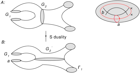
Figure 20: S duality action on a theory defined on a torus with two punctures, and the dual gauge group $G_{2}^{{}^{\prime}}$ depends on the choice of gauge group $G_{1}$.

No essentially new things happen if we consider theory defined by a genus one Riemann surface with arbitrary number of punctures.

5.3.4 Genus two case

Let’s consider a four dimensional theory defined on a genus two Riemann surface without any puncture, and this class of theory is first studied by Maldacena and Nunez [35]. The first homology group is generated by $([a_{1}],[a_{2}])$ and $([b_{1}],[b_{2}])$, and the intersection numbers are

$$[a_{1}]\cdot[b_{1}]=1,~{}~{}[a_{2}]\cdot[b_{2}]=1.$$ (49)

Now let’s discuss the choice of line operators. First, we need to take a maximal set of non-intersecting basis, and here we take them to be $[a_{1}]$ and $[a_{2}]$, then the classification is done as:

• The choice of electric homology class is the same as genus one case we just studied, and the basis can be denoted as

  $$e_{1}=n_{1}k_{1}[a_{1}],~{}~{}~{}~{}~{}~{}e_{2}=n_{2}k_{2}[a_{2}],$$ (50)

  and here $k_{1}$ and $k_{2}$ satisfies the condition $k_{1}k_{1}^{{}^{\prime}}=N$ and $k_{2}k_{2}^{{}^{\prime}}=N$.

• Let’s denote the homology class of pure magnetic line operator as $m_{1}[b_{1}]+m_{2}[b_{2}]$, then the mutual locality condition implies that

  $$m_{1}=p_{1}k_{1}^{{}^{\prime}},~{}~{}m_{2}=p_{2}k_{2}^{{}^{\prime}}.$$ (51)

• For a general homology class $[L]=q_{1}[a_{1}]+q_{2}[a_{2}]+m_{1}[b_{1}]+m_{2}[b_{2}]$, mutual locality condition with the electric and magnetic line operators simply implies

  $$[L]=n_{1}k_{1}[a_{1}]+n_{2}k_{2}[a_{2}]+p_{1}k_{1}^{{}^{\prime}}[b_{1}]+p_{2}k_{2}^{{}^{\prime}}[b_{2}].$$ (52)

Now let’s interpret the classification in terms of gauge theory. Let’s start with a weakly coupled duality frame represented by pants decomposition determined by three closed curves: $K_{1},K_{2},K_{3}$. This pants decomposition can be thought of first cutting the Riemann surface by $K_{1}$ and $K_{2}$, and get a fourth punctured sphere which is further cut into two pants by $K_{3}$. Here $K_{1}$ is in homology class $[a_{1}]$, and $K_{2}$ is in homology class $[a_{2}]$ and $K_{3}$ is in trivial homology class.

According to our rules discussed earlier, the global form of gauge groups in the above duality frame are simple, and they are

$$K_{1}:~{}~{}{SU(N)\over Z_{k_{1}}},~{}~{}~{}~{}~{}~{}K_{2}:~{}~{}{SU(N)\over Z_{k_{2}}},~{}~{}~{}~{}K_{3}:~{}~{}SU(N)$$ (53)

We can do $T$ duality on $K_{1}$ and $K_{2}$ to find different sets of allowed set of line operators, and the details is the same as the genus one case. The $T$ transformation around $K_{1}$ change the homology class of line operators as

$$T_{1}:~{}~{}n_{1}k_{1}[a_{1}]+n_{2}k_{2}[a_{2}]+p_{1}k_{1}^{{}^{\prime}}[b_{1}]+p_{2}k_{2}^{{}^{\prime}}[b_{2}]\rightarrow(n_{1}k_{1}+p_{1}k_{1}^{{}^{\prime}})[a_{1}]+n_{2}k_{2}[a_{2}]+p_{1}k_{1}^{{}^{\prime}}[b_{1}]+p_{2}k_{2}^{{}^{\prime}}[b_{2}]$$

$$T_{2}:~{}~{}n_{1}k_{1}[a_{1}]+n_{2}k_{2}[a_{2}]+p_{1}k_{1}^{{}^{\prime}}[b_{1}]+p_{2}k_{2}^{{}^{\prime}}[b_{2}]\rightarrow n_{1}k_{1}[a_{1}]+(n_{2}k_{2}+p_{2}k_{2}^{{}^{\prime}})[a_{2}]+p_{1}k_{1}^{{}^{\prime}}[b_{1}]+p_{2}k_{2}^{{}^{\prime}}[b_{2}]$$

$$T_{3}:~{}~{}n_{1}k_{1}[a_{1}]+n_{2}k_{2}[a_{2}]+p_{1}k_{1}^{{}^{\prime}}[b_{1}]+p_{2}k_{2}^{{}^{\prime}}[b_{2}]\rightarrow n_{1}k_{1}[a_{1}]+n_{2}k_{2}[a_{2}]+p_{1}k_{1}^{{}^{\prime}}[b_{1}]+p_{2}k_{2}^{{}^{\prime}}[b_{2}]$$ (54)

What is interesting is to do S duality on $K_{3}$ and the dual theory is described by three closed curves $K_{1},K_{2},K_{3}^{{}^{\prime}}$. Unlike $K_{3}$, $K_{3}^{{}^{\prime}}$ is in non-trivial homology class $[a_{1}]-[a_{2}]$. Since we have chosen the minimal winding around $[a_{1}]$ and $[a_{2}]$, and we can find the gauge group around $K_{3}^{{}^{\prime}}$ using the rules in last subsection. The $T$ transformation around $T_{3}$ is nontrivial now:

$$T_{3}:~{}~{}n_{1}k_{1}[a_{1}]+n_{2}k_{2}[a_{2}]+p_{1}k_{1}^{{}^{\prime}}[b_{1}]+p_{2}k_{2}^{{}^{\prime}}[b_{2}]\rightarrow$$

$$(n_{1}k_{1}+p_{1}k_{1}^{{}^{\prime}})[a_{1}]+(n_{2}k_{2}-p_{2}k_{2}^{{}^{\prime}})[a_{2}]+p_{1}k_{1}^{{}^{\prime}}[b_{1}]+p_{2}k_{2}^{{}^{\prime}}[b_{2}]$$ (55)

However, it is easy to see $T_{3}=T_{1}T_{2}^{-}$ and the Dehn twist around the circle $K_{3}^{{}^{\prime}}$ will not generate new theories. So it is enough to consider $T$ transformation around $a_{1}$ and $a_{2}$. All possible choices of theories for $A_{1}$ theory is shown in figure. 22, and the duality webs relating these theories can be easily found using our formula for $S$ and $T$ transformation, see figure. 23.

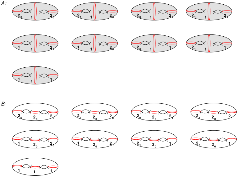
Figure 22: Up: Different gauge theories associated with one duality frame. Bottom: Different gauge theories associated with another duality frame.

Figure 23: Duality webs relating different gauge theories.

5.3.5 Arbitrary genus

For a genus $g$ Riemann surface without punctures (the puncture case does not introduce new features), the pants decomposition can be thought of as two steps: (1): Choose $g$ non-separating closed curves $c_{i}$ to cut the Riemann surface into a punctured sphere; (2): Choose a pants decomposition of punctured sphere. It is easy to see that $c_{i}$ is a maximal set of commuting basis for the homology class. See figure. 24 for a basis of homology group, and one can choose $a_{i}$ as a maximal set of commuting non-separating cut system.

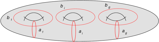
Figure 24: Basis for homology group of a genus $g$ Riemann surface.

To classify the line operators, we do the following: (1): Choose the minimal line operators around $c_{i}$; (2) The homology class of pure magnetic line operators (by pure magnetic line operators we mean line operators in homology class generated by basis not included in $(1)$) by imposing locality condition with the homology class chosen in (1); (3) Find the mixed line operator imposing the locality condition with sets (1) and (2). Again, there are only $g$ discrete ndependent $\theta$ angles.

The above choices can be regarded as taking zero $\theta$ angle for all the gauge groups. To find the allowed line operators for non-zero $\theta$ angles, we simply do $T$ transformation on various gauge groups, which will typically mix the electric and magnetic homology classes. The choice of line operators will be very rich.

One can use our general formula of $T$ and $S$ transformation to relate different kinds of theories, and we leave the details to interested reader.

6 Conclusion

We studied various aspects of line operators of class ${\cal S}$ theory: we identify the geometric representations of Wilson-’t Hooft line operators and study the duality actions on them. We define the mutual locality condition on line operators. Then we use closure of OPE, mutual locality and maximality conditions to classify the allowed set of line operators. Finally we study the duality actions relating different gauge theories. The geometrical construction of line operators plays a crucial role in our applications.

There is one interesting lesson we learn about the choice of discrete $\theta$ angles: one can not choose them independently and there are intricate relations among the choice of $\theta$ angles as we show for genus two example. This interesting feature is related to the property of duality group or mapping class group. The topology of conformal manifold is entirely encoded in the property of mapping class group, and it does have important effects on the choice of discrete $\theta$ angles. It is interesting to further study the mapping class group (duality group) using line operators.

We only consider 4d theory derived using 6d $A_{N-1}$ theory with full punctures, and it is interesting to generalize the study to more general case, i.e theory defined using non-full punctures. It is also interesting to generalize the consideration to D and E type theories.

We look at the classification of line operators using the geometric objects on the Riemann surface. The main reason is that these geometric objects are natural space on which duality action acts. We do not touch too much on four dimensional gauge theory meaning except the interpretation of discrete $\theta$ angle. It is pointed out in [20] that such choice of line operators has important implication for the physical theory derived by compactifying four dimensional theory on a circle (see [36] for further study using index calculation.). What we want to point out is that the line operators in our picture also related to the four dimensional theory on a circle. In fact, the line operator in our case describes the canonical basis on the moduli space of Hitchin equation which actually describes the Coulomb branch of four dimensional theory reduced on a circle. Given different choices of line operators, we actually get different moduli space, therefore our choice of line operators indeed reflects the vacuum structure of four dimensional theory on a circle.

Moreover, these line operators are related to the Hamiltonian of the underlying Hitchin integrable system, and the quantization of this integrable system is related to the Nekrasov partition function of the gauge theory. It is interesting to see how the choice of line operators would affect the partition functions.

Similar 6d construction for a large class of $\mathcal{N}=1$ theories is presented in [37], and we have a generalized Hitchin equation in that context. It is natural to think of line operators of $\mathcal{N}=1$ theory in terms of closed curves on Riemann surface, and define its expectation value in terms of monodromy of commuting flat connections derived from generalized Hitchin equation. Although there is no BPS line operators of $\mathcal{N}=1$ theory, it is still possible to use the geometric construction to learn interesting dynamics of $\mathcal{N}=1$ theory, and we would like to report the progress in that direction in the near future.

Acknowledgments

We thank Vasily Pestun, Shlomo Razamat, Yuji Tachikawa, Nathan Seiberg, Brian Willet, Kazuya Yonekura and Peng Zhao for helpful discussions. This research is supported in part by Zurich Financial services membership and by the U.S. Department of Energy, grant DE-SC0009988 (DX).

Appendix A A proof that mutual locality condition is independent of coordinate system

The Dirac product between two line operators $L_{1}$ and $L_{2}$ are defined as the coefficient of the leading order term in Poisson bracket of two line operators. Let’s denote the tropical $a$ coordinates of $L_{1}$ as $a_{1i}$ and tropical $x$ coordinates of $L_{2}$ as $x_{2i}$. An important fact is that the dual $x$ coordinates are always integer. The Dirac product of two line operators is simply

$$<L_{1},L_{2}>=-\sum_{k}x_{1k}a_{2k}.$$ (56)

Let’s do a mutation on a a quiver node $i$, then after the mutation, the tropical $a$ coordinates become

$$a_{i}^{{}^{\prime}}=-a_{i}+\text{max}([{{\epsilon_{ij}}]_{+}a_{j},[{\epsilon_{ij}}]_{-}a_{j}}),$$ (57)

here $\epsilon_{ij}$ is the antisymmetric tensor of the quiver; and the tropical $x$ coordinates become

$$x_{i}^{{}^{\prime}}=-x_{i}$$

$$x_{j}^{{}^{\prime}}=x_{j}+\epsilon_{ji}\text{max}(0,\text{sgn}(\epsilon_{ji})x_{i})$$ (58)

The new intersection number is then

$$<L_{1},L_{2}>=-\sum_{k}x_{1k}^{{}^{\prime}}a_{2k}^{{}^{\prime}}=-\sum x_{1k}a_{2k}+(\pm x_{1i}x_{2i}~{}\text{or}~{}0).$$ (59)

since the dual $x$ coordinates are always integer, the Dirac product has the same fraction number behavior in new coordinate system. Therefore if two line operators are mutually local in one coordinate system, they will be mutually local in any coordinate system related by cluster transformation.

References

- [1] P. C. Argyres and M. R. Douglas, “New phenomena in SU(3) supersymmetric gauge theory,” Nucl.Phys. B448 (1995) 93–126, arXiv:hep-th/9505062 [hep-th].
- [2] P. C. Argyres, M. Ronen Plesser, N. Seiberg, and E. Witten, “New N=2 superconformal field theories in four-dimensions,” Nucl.Phys. B461 (1996) 71–84, arXiv:hep-th/9511154 [hep-th].
- [3] D. Gaiotto, “ dualities,” arXiv:0904.2715 [hep-th].
- [4] D. Gaiotto, G. W. Moore, and A. Neitzke, “Wall-crossing, hitchin Systems, and the WKB approximation,” arXiv:0907.3987 [hep-th].
- [5] D. Xie, “General Argyres-Douglas Theory,” arXiv:1204.2270 [hep-th].
- [6] O. Chacaltana, J. Distler, and Y. Tachikawa, “Nilpotent orbits and codimension-two defects of 6d N=(2,0) theories,” Int.J.Mod.Phys. A28 (2013) 1340006, arXiv:1203.2930 [hep-th].
- [7] P. C. Argyres and N. Seiberg, “S-Duality in supersymmetric gauge theories,” JHEP 12 (2007) 088, arXiv:0711.0054 [hep-th].
- [8] N. Drukker, D. R. Morrison, and T. Okuda, “Loop operators and S-duality from curves on Riemann surfaces,” JHEP 09 (2009) 031, arXiv:0907.2593 [hep-th].
- [9] D. Gaiotto, G. W. Moore, and A. Neitzke, “Framed BPS states,” arXiv:1006.0146 [hep-th].
- [10] R. Penner, “Probing mapping class groups using arcs,” in PROCEEDINGS OF SYMPOSIA IN PURE MATHEMATICS, vol. 74, p. 97, Providence, RI; American Mathematical Society; 1998. 2006.
- [11] D. Xie, “Higher laminations, webs and N=2 line operators,” arXiv:1304.2390 [hep-th].
- [12] N. Drukker, D. Gaiotto, and J. Gomis, “The Virtue of Defects in 4D Gauge Theories and 2D CFTs,” JHEP 1106 (2011) 025, arXiv:1003.1112 [hep-th].
- [13] J. Gomis and B. Le Floch, “’t Hooft Operators in Gauge Theory from Toda CFT,” JHEP 1111 (2011) 114, arXiv:1008.4139 [hep-th].
- [14] Y. Ito, T. Okuda, and M. Taki, “Line operators on S1xR3 and quantization of the Hitchin moduli space,” JHEP 1204 (2012) 010, arXiv:1111.4221 [hep-th].
- [15] D. Gang, E. Koh, and K. Lee, “Line Operator Index on ,” JHEP 1205 (2012) 007, arXiv:1201.5539 [hep-th].
- [16] M. Cirafici, “Line defects and (framed) BPS quivers,” JHEP 1311 (2013) 141, arXiv:1307.7134 [hep-th].
- [17] C. Cordova and A. Neitzke, “Line Defects, Tropicalization, and Multi-Centered Quiver Quantum Mechanics,” arXiv:1308.6829 [hep-th].
- [18] Y. Tachikawa, “On the 6d origin of discrete additional data of 4d gauge theories,” arXiv:1309.0697 [hep-th].
- [19] A. Kapustin, “Wilson-’t Hooft operators in four-dimensional gauge theories and S-duality,” Phys.Rev. D74 (2006) 025005, arXiv:hep-th/0501015 [hep-th].
- [20] O. Aharony, N. Seiberg, and Y. Tachikawa, “Reading between the lines of four-dimensional gauge theories,” JHEP 1308 (2013) 115, arXiv:1305.0318 [hep-th].
- [21] D. Xie, “Network, cluster coordinates and N = 2 theory II: Irregular singularity,” arXiv:1207.6112 [hep-th].
- [22] O. Lunin, “1/2-BPS states in M theory and defects in the dual CFTs,” JHEP 0710 (2007) 014, arXiv:0704.3442 [hep-th].
- [23] B. Chen, W. He, J.-B. Wu, and L. Zhang, “M5-branes and Wilson Surfaces,” JHEP 0708 (2007) 067, arXiv:0707.3978 [hep-th].
- [24] E. D’Hoker, J. Estes, and M. Gutperle, “Exact half-BPS Type IIB interface solutions. II. Flux solutions and multi-Janus,” JHEP 0706 (2007) 022, arXiv:0705.0024 [hep-th].
- [25] D. Xie, “Network, Cluster coordinates and N=2 theory I,” arXiv:1203.4573 [hep-th].
- [26] V. V. Fock and A. B. Goncharov, “Moduli spaces of local systems and higher teichmuller theory,”. \urlarXiv.org:math/0311149.
- [27] A. Kapustin and E. Witten, “Electric-Magnetic Duality And The Geometric Langlands Program,” Commun.Num.Theor.Phys. 1 (2007) 1–236, arXiv:hep-th/0604151 [hep-th].
- [28] A. Kapustin and N. Saulina, “The Algebra of Wilson-’t Hooft operators,” Nucl.Phys. B814 (2009) 327–365, arXiv:0710.2097 [hep-th].
- [29] N. Saulina, “A note on Wilson-’t Hooft operators,” Nucl.Phys. B857 (2012) 153–171, arXiv:1110.3354 [hep-th].
- [30] R. Moraru and N. Saulina, “OPE of Wilson-’t Hooft operators in N=4 and N=2 SYM with gauge group G=PSU(3),” arXiv:1206.6896 [hep-th].
- [31] D. Xie and P. Zhao, “Algebra of line operators,” Work in progress .
- [32] E. Witten, “Dyons of charge e/2,” Physics Letters B 86 (1979) no. 3, 283–287.
- [33] A. Hatcher and W. Thurston, “A presentation for the mapping class group of a closed orientable surface,” Topology 19 (1980) no. 3, 221–237.
- [34] B. Farb and D. Margalit, A Primer on Mapping Class Groups (PMS-49). Princeton University Press, 2011.
- [35] J. M. Maldacena and C. Nunez, “Supergravity description of field theories on curved manifolds and a no go theorem,” Int.J.Mod.Phys. A16 (2001) 822–855, arXiv:hep-th/0007018 [hep-th].
- [36] S. S. Razamat and B. Willett, “Global Properties of Supersymmetric Theories and the Lens Space,” arXiv:1307.4381 [hep-th].
- [37] D. Xie, “M5 brane and four dimensional N=1 theories I,” arXiv:1307.5877 [hep-th].