Radiation Transfer of Models of Massive Star Formation. III. The Evolutionary Sequence

Abstract

We present radiation transfer simulations of evolutionary sequences of massive protostars forming from massive dense cores in environments of high mass surface densities, based on the Turbulent Core model (McKee & Tan 2003). The protostellar evolution is calculated with a multi-zone numerical model, with accretion rate regulated by feedback from an evolving disk-wind outflow cavity. Disk evolution is calculated assuming a fixed ratio of disk to protostellar mass, while core envelope evolution assumes inside-out collapse of the core of fixed outer radius. In this framework, an evolutionary track is determined by three environmental initial conditions: core mass $M_{c}$, mass surface density of the ambient clump $\Sigma_{\rm cl}$, and ratio of the core’s initial rotational to gravitational energy $\beta_{c}$. Evolutionary sequences with various $M_{c}$, $\Sigma_{\rm cl}$, $\beta_{c}$ are constructed. We find that in a fiducial model with $M_{c}=60\;M_{\odot}$, $\Sigma_{\rm cl}=1\;{\rm g}\,{\rm cm}^{-2}$ and $\beta_{c}=0.02$, the final mass of the protostar reaches at least $\sim 26\;M_{\odot}$, making the final star formation efficiency $\gtrsim 0.43$. For each of the evolutionary tracks, radiation transfer simulations are performed at selected stages, with temperature profiles, spectral energy distributions (SEDs), and multi-wavelength images produced. At a given stage, envelope temperature is depends strongly on $\Sigma_{\rm cl}$, with higher temperatures in a higher $\Sigma_{\rm cl}$ core, but only weakly on $M_{c}$. The SED and MIR images depend sensitively on the evolving outflow cavity, which gradually widens as the protostar grows. The fluxes at $\lesssim 100\;\mu$m increase dramatically, and the far-IR peaks move to shorter wavelengths. The influence of $\Sigma_{\rm cl}$ and $\beta_{c}$ (which determines disk size) are discussed. We find that, despite scatter caused by different $M_{c}$, $\Sigma_{\rm cl}$, $\beta_{c}$, and inclinations, sources at a given evolutionary stage appear in similar regions of color-color diagrams, especially when using colors with fluxes at $\gtrsim 70\>\mu$m, where scatter due to inclination is minimized, implying that such diagrams can be useful diagnostic tools of evolutionary stages of massive protostars. We discuss how intensity profiles along or perpendicular to the outflow axis are affected by environmental conditions and source evolution, and can thus act as additional diagnostics of the massive star formation process.

1. Introduction

Massive stars impact many areas of astrophysics, yet there is still no consensus on how they form. One possible scenario is that they form in a similar way to low-mass stars, i.e. through accretion from gravitationally bound cores (Core Accretion). In the Turbulent Core model (McKee & Tan 2002, 2003, hereafter MT02, MT03), the massive cores that will form massive stars are supported by internal pressure provided by a combination of turbulence and magnetic fields. The pressure at the core surface is assumed to be approximately the same as that of the surrounding larger-scale self-gravitating star-cluster-forming clump, with a typical mean mass surface density of $\Sigma_{\rm cl}=1\>{\rm g}\,{\rm cm}^{-2}$. Such dense and highly pressurized cores can reach high accretion rates during their collapse, which may be needed to form massive stars. Depending on how, including how quickly, the initial massive starless core is assembled and how much additional material is accreted during collapse, such a scenario may involve relatively ordered, monolithic accretion via a central disk and the driving of collimated bipolar outflows. Other possible mechanisms include Competitive Accretion (e.g., Bonnell et al. 2001; Wang et al. 2010), and Stellar Collisions (e.g., Bonnell et al. 1998), which involve much less ordered and chaotic accretion processes (see, e.g., Tan et al. 2014, for a recent review).

If core accretion is how massive stars form, the evolution of massive protostellar objects should be dependent on the initial conditions of the cores. The Turbulent Core model explicitly relates the structure and the evolution of a core to two initial conditions: the initial mass of the core $M_{c}$ and the mean mass surface density of the surrounding clump $\Sigma_{\rm cl}$. In addition, the disk size is expected to be dependent on the degree of rotation in the initial core, which can be described by the parameter $\beta_{c}$, the ratio of the rotational energy to the gravitational energy of a core.

It is difficult to observationally identify the evolutionary stages of massive protostars due to the fact that they form in very crowded, highly obscured, and distant environments. Therefore, in order to more accurately estimate the properties of massive young stellar objects (YSOs) and constrain the theories of massive star formation, radiative transfer (RT) calculations are needed to predict the spectral energy distribution (SED) and images to compare with multiwavelength observations of massive YSOs. A number of RT models have been developed to compare with the observations. Robitaille et al. (2006) developed a large model grid to fit YSO SEDs. In particular, they found that the spectral index or color calculated with fluxes at $\gtrsim 20\>\mu$m is valuable for deriving the evolutionary stages of YSOs. However their model grid was mainly developed for low-mass star formation, without coverage of the parameter space needed for massive star formation, such as very high accretion rates or massive compact cores expected in high surface density environments. Also, the components in the model are relatively simple (e.g., the density in the outflow is usually assumed to be either a constant value or a power law) and not self-consistently included based on the evolutionary sequences. Furthermore, gas opacities, relevant for the region inside the dust destruction front, where most accretion power is liberated, were not included. A similar RT model grid has also been developed by Molinari et al. (2008), focused on MYSOs. Their results from fitting the observations with this model grid suggested there are two groups of sources occupying different regions in the color-color diagram at 24 $\mu$m and longer wavelengths and the mass-luminosity diagram, which may represent two evolutionary stages of massive star formation. However, the components in their model are also relatively simple and there is no self-consistent protostellar evolution included.

Here we present the third of a series of papers on modeling the spectral energy distributions (SEDs) and images of massive protostars, forming from massive gas cores under the paradigm of the Turbulent Core Model. In the previous papers (Zhang & Tan 2011, hereafter Paper I; Zhang et al. 2013a, here after Paper II), we studied a star-forming core with an initial mass of $60\>M_{\odot}$ at the particular moment that the protostar reaches $8\>M_{\odot}$. We self-consistently included an active accretion disk allowing a supply of mass and angular momentum from the infall envelope and their loss to a disk wind, developed an approximate disk wind solution, and also included the corrections made by gas opacities, adiabatic cooling/heating and advection. A variant of this fiducial model has been used to successfully explain the multiwavelength observations (both global SED and multiwavelength intensity profiles along the outflow axis) of a massive protostar G35.2-0.74N (Zhang et al. 2013b). In this paper, extending the model developed in Paper I and Paper II, we shall construct the evolutionary sequences of massive protostars, self-consistently from the specific initial environmental conditions of the pre-stellar core discussed above. We first assume a constant star formation efficiency (the ratio of the stellar accretion rate to the ideal collapsing rate of the core assuming no feedback) of half as in previous papers, but then introduce a new estimate for an evolving efficiency based on an analytic model of the disk wind outflow and its feedback on the core. As the outflow gradually opens up bipolar cavities, the instantaneous star formation efficiency decreases with time. We also improve the treatment of protostellar evolution with a detailed protostellar evolution code, which then utilizes the self-consistently calculated stellar accretion rate that is controlled by the formation efficiency. We present radiation transfer calculations of these models and their variants with different initial conditions at selected evolutionary stages. We discuss the model setup in Section 2, and present the results of our models in Section 3. In Section 4, we discuss the possible effects of including the ambient clump material in the RT simulation, and how that affects the modeling of observations. We summarize our main conclusions in Section 5.

2. Models

We first briefly describe those aspects of the model setup from our previous works that we will continue to use (for details see Paper I and II), before discussing the new features in the following subsections. Following MT03, a star-forming core is defined as a region of a molecular cloud that forms a single star or a close binary via gravitational collapse. The core is assumed to be spherical, self-gravitating, in near virial equilibrium, and in pressure equilibrium with the surrounding clump. In the fiducial case, we study a core with $M_{c}=60\>M_{\odot}$. The size of such a core is determined by the mean mass surface density of the clump $\Sigma_{\rm cl}$ (which sets the pressure on the boundary of the core) by $R_{c}=5.7\times 10^{-2}(M_{c}/60\>M_{\odot})^{1/2}(\Sigma_{\rm cl}/{\rm g}\,{\rm cm}^{-2})^{-1/2}\>\mathrm{pc}$ (i.e. $R_{c}=1.2\times 10^{4}$ AU in the fiducial case with $M_{c}=60\>M_{\odot}$ and $\Sigma_{\rm cl}=1\>{\rm g}\,{\rm cm}^{-2}$). We also consider variants of this model with several different values of $M_{c}$, $\Sigma_{\rm cl}$, and the rotational energy which sets the disk size (see Section 2.1), forming a small grid of models. These relations are based on the assumption of a singular polytropic core, which is consistent with observations of dense cores in Infrared Dark Clouds. Such observations suggest the density distribution in the core can be described by a power law in spherical radius, $\rho\propto r^{-k_{\rho}}$, with the mean value of $k_{\rho}$ estimated to be $\simeq$1.3 to 1.6 (Butler & Tan 2012, Butler et al. 2014). Following Paper I and II, a fiducial value $k_{\rho}=1.5$ is used here.

The collapse of the core is described with an inside-out expansion wave solution (Shu 1977; McLaughlin & Pudritz 1997), which is the expected collapse evolution of a singular polytropic sphere, although it is challenging to resolve such infall profiles around actual massive protostars (Tan et al. 2014). The effects of rotation on the velocity field and the density profile are described with the solution by Ulrich (1976) (see also Tan & McKee 2004). The disk around a massive protostar can have a high mass. In all our models, we assume the mass ratio between the disk and the protostar is a constant $f_{d}=m_{d}/m_{*}=1/3$, considering the rise in effective viscosity due to disk self-gravity at about this value of $f_{d}$ (Kratter et al. 2008). The disk structure is described with an “$\alpha$-disk” solution (Shakura & Sunyaev 1973), with an improved treatment to include the effects of the outflow and the accretion infall to the disk (Paper II). The corresponding $\alpha$ varies from $\sim 0.02$ to $\sim 0.07$ in the fiducial model, given the constant disk-to-stellar mass ratio and the disk size (see 2.1). Half of the accretion energy is released when the accretion flow reaches the stellar surface (the boundary layer luminosity $L_{\mathrm{acc}}=Gm_{*}\dot{m}_{*}/(2r_{*})$), but we assume this part of luminosity is radiated along with the stellar luminosity isotropically as a single black-body ($L_{*,\mathrm{acc}}=L_{*}+L_{\mathrm{acc}}$), i.e. we typically assume that there is minimal advection of gravitational energy into the star (see Section 2.2). The other half of the accretion energy is partly radiated from the disk and partly converted to the kinetic energy of the disk wind.

The density distribution in the outflow cavity is described by a semi-analytic disk wind solution which is approximately a Blandford & Payne (1982) (hereafter BP) wind (see Appendix B of Paper II), and the mass loading rate of the wind relative to the stellar accretion rate is assumed to be $f_{w}=\dot{m}_{w}/\dot{m}_{*}=0.1$ which is a typical value for disk winds (Königl & Pudritz 2000). Instead of assuming a fixed opening angle of the outflow cavity to reach an assumed star formation efficiency of half (as we did in Papers I and II), in this paper we study the evolution of the outflow cavity.

2.1. Rotation of the Initial Core and Growth of the Disk

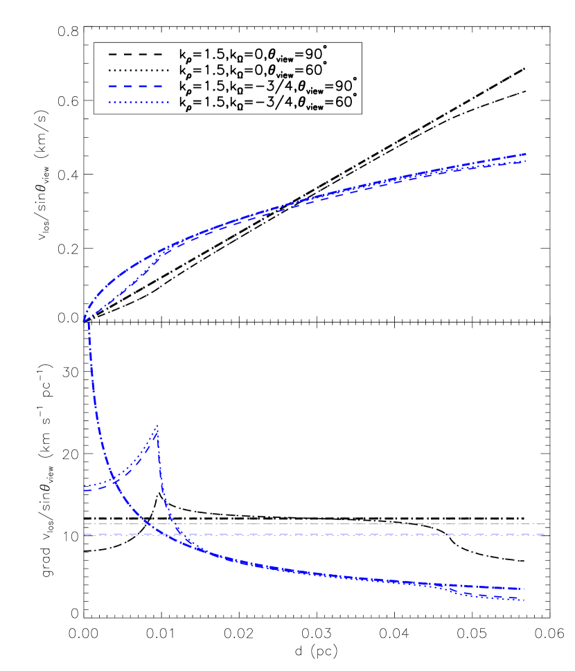
Figure 1.— The profiles of line-of-sight velocities (upper panel) and their gradients (lower panel) with the projected distance from the rotational axis. All the models assume $M_{c}=60\>M_{\odot},\Sigma_{\rm cl}=1\>{\rm g}\,{\rm cm}^{-2}$, and $\beta_{c}=0.02$. The black curves are for a case of solid-rotating core, and the blue curves are for the case with $k_{\Omega}=-k_{\rho}/2$ to make a constant $\beta_{c}$ profile. The dashed and dotted curves are for different viewing inclinations (they sometimes coincide). Note the y axes are scaled by $\sin\theta_{\mathrm{view}}$. The velocities are mass-weighted and averaged along the line of sight and also over sky plane in two ways. The most thick lines are averaged along a strip with infinite resolution in $d$ and width of core size, the lines with intermediate thickness are averaged over a circular resolution beam of 4000 AU (4$\arcsec$ in 1 kpc). Following Goodman et al. (1993), we also derive a gradient level using 2D linear fitting, which are marked with the most thin lines.

The rotation of the core is usually described with the parameter $\beta$, the rotational-to-graviational energy ratio in the core. Inside any radius $r$ in a polytropic core, we have

$$\beta(<r)\propto M(<r)^{-1}r^{3}\Omega(r)^{2}\propto r^{k_{\rho}+2k_{\Omega}}.$$ (1)

where $M(<r)$ is the mass inside $r$, and we assume a power-law profile of $\Omega\propto r^{k_{\Omega}}$. In general cases, $k_{\rho}\neq 0$, if the core is rotating as a solid body ($k_{\Omega}=0$), $\beta(<r)$ has a dependence on radius. Only when $k_{\Omega}=-k_{\rho}/2$, does $\beta$ becomes a constant, $\beta=\beta_{c}\equiv\beta(<R_{c})$.

Observationally, $\beta_{c}$ is derived by measuring the velocity gradient over the core (e.g., Goodman et al. 1993), and usually with assumptions that $k_{\rho}=0$ and $k_{\Omega}=0$. Based on observations of both low-mass and high-mass cores, $\beta_{c}$ is found to have a typical value of 0.02 and range from $\sim$0.001 to $\sim$0.2 (e.g., Goodman et al. 1993, Li et al. 2012, Palau et al. 2013). Therefore we choose a fiducial value of 0.02 for $\beta_{c}$. The profile of line-of-sight velocity $v_{\mathrm{los}}$ with projected distance $d$ to the rotational axis can be written as

$$v_{\mathrm{los}}=d\sin\theta_{\mathrm{view}}\sqrt{\frac{GM_{c}\beta_{c}}{R_{c}^{3}}}V(d,k_{\rho},k_{\Omega},\theta_{\mathrm{view}}),$$ (2)

where $\theta_{\mathrm{view}}$ is the inclination angle between the rotational axis and the line of sight. The averaging effects of the velocity along the line of sight and over finite spatial resolutions are included in the factor $V$. We note that the line-of-sight velocity and its gradient are proportional to $\sqrt{M_{c}\beta_{c}/R_{c}^{3}}\propto\beta_{c}^{1/2}M_{c}^{-1/4}\Sigma_{\rm cl}^{3/4}$.

In Figure 1, we show the line-of-sight velocities and their gradients with the projected distance from the rotational axis for the fiducial initial core ($M_{c}=60M_{\odot}$, $\Sigma_{\rm cl}=1\>{\rm g}\,{\rm cm}^{-2}$, $k_{\rho}=1.5$, $\beta_{c}=0.02$). Profiles for different $k_{\Omega}$ and inclinations are shown. Note that the y axes are velocity or gradient scaled by $\sin\theta_{\mathrm{view}}$. In most of cases, $V$ is only weakly dependent on $\theta_{\mathrm{view}}$. 2D linearly fitted gradients following the method of Goodman et al. (1993) are also shown. For models with different rotation curves, the fitted gradients are actually similar, at a level of $\sim 10$ km/s/pc, which is higher than most of the observed values in the literatures mentioned above (although similar gradient level has been observed in some cases, e.g., Chen et al. 2012), maybe because of the lower $\Sigma_{\rm cl}$ of the environments of their prestellar core samples. Detailed rotation curves and $\beta$ profiles can be derived from observations with better spatial and velocity resolutions.

If we assume the angular momentum is conserved inside the sonic point of the inflow, we have

$$\Omega_{d}=\left(\frac{Gm_{*d}}{r_{d}^{3}}\right)^{1/2}=\Omega_{\mathrm{sp}}\left(\frac{r_{\mathrm{sp}}}{r_{d}}\right)^{2},$$ (3)

where $m_{*d}$ is the total mass of the star and disk, and $\Omega_{\mathrm{sp}}$ is the angular velocity when reaching the sonic point. This gives the size of the disk as the maximum centrifugal radius,

$$r_{d}=\frac{\Omega_{\mathrm{sp}}^{2}r_{\mathrm{sp}}^{4}}{Gm_{*d}}.$$ (4)

Therefore, in order to calculate $r_{d}$ at the moment that the collapsed mass (the ideal star + disk mass in the case of no feedback, i.e. star formation efficiency of unity) is $M_{*d}$, we need to know the radius where a shell enclosing that mass becomes supersonic in the past of the collapse, $r_{\mathrm{sp}}(M_{*d})$, and the initial angular velocity $\Omega_{\mathrm{sp}}(M_{*d})$.

The shell enclosing mass $M_{*d}$ originally is at radius

$$r_{0}(M_{*d})=\left(\frac{M_{*d}}{M_{c}}\right)^{\frac{1}{3-k_{\rho}}}R_{c}$$ (5)

for a polytropic core. And the ratio between the radius where this shell reaches a supersonic infall velocity and its original radius is given by the expansion wave solution (see appendix of McLaughlin & Pudritz 1997),

$$\frac{r_{\mathrm{sp}}}{r_{0}}=\left(\frac{x_{\mathrm{sp}}}{x_{\mathrm{ew}}}\right)\left(\frac{m_{0}}{m_{\mathrm{sp}}}\right)^{\frac{1}{3-k_{\rho}}}\left(\frac{t_{f}}{t_{\mathrm{ew}}}\right)^{\frac{2}{k_{\rho}}},$$ (6)

where $x_{\mathrm{sp}}$ and $x_{\mathrm{ew}}$ are the dimensionless radii of the sonic point and the expansion wave in the self-similar expansion wave solution, $m_{0}$ and $m_{\mathrm{sp}}$ are the dimensionless masses at the center and inside the sonic point, $t_{f}$ and $t_{\mathrm{ew}}$ are the times for the core to collapse and for the expansion wave to reach the core boundary, respectively. Given by the expansion wave solution, these parameters are only dependent on $k_{\rho}$. In our case, with $k_{\rho}=1.5$, we have $x_{\mathrm{sp}}=0.151$, $x_{\mathrm{ew}}=0.595$, $m_{0}=0.124$, $m_{\mathrm{sp}}=0.154$, $t_{\mathrm{ew}}/t_{f}=0.469$, leading to $r_{\mathrm{sp}}/r_{0}=0.601$.

For the initial polytropic core, for any $r$, we can write the following for the gravitational and rotational energy inside that radius,

$$|E_{\mathrm{grav}}|=a_{g}\left[\frac{3GM(<r)^{2}}{5r}\right],$$ (7)

$$E_{\mathrm{rot}}=a_{i}\left[\frac{1}{2}M(<r)r^{2}\bar{\Omega}(<r)^{2}\right],$$ (8)

with $a_{g}=(5/3)(3-k_{\rho})/(5-2k_{\rho})$ ($\rightarrow 5/4$ in the fiducial case with $k_{\rho}=3/2$) and $a_{i}=(2/3)(3-k_{\rho})/(5-k_{\rho})$ ($\rightarrow$0.286 in the fiducial case). Therefore the averaged angular velocity $\bar{\Omega}$ inside $r$ is

$$\bar{\Omega}(<r)^{2}=\frac{6a_{g}}{5a_{i}}\beta(<r)\frac{GM(<r)}{r^{3}}.$$ (9)

We assume a constant $\beta$ profile, $\beta(<r)=\beta_{c}$, and use $\bar{\Omega}[<r_{0}(M_{*d})]$ as an estimation of $\Omega_{\mathrm{sp}}(M_{*d})$.

We then are able to write Equation 4 as

$$r_{d}(M_{*d})=0.684\>\beta_{c}\left(\frac{M_{*d}}{m_{*d}}\right)\left(\frac{M_{*d}}{M_{c}}\right)^{\frac{2}{3}}R_{c}.$$ (10)

This formula indicates that the size of the disk depends on the size of the core $R_{c}$, the rotational energy fraction of the core $\beta_{c}$, the averaged efficiency ($m_{*d}/M_{*d}$), and evolves with time as $M_{*d}/M_{c}$. If we do not use the averaged $\Omega$ inside of some radius as $\Omega_{\mathrm{sp}}$, we will have an additional factor of about 2 increase for the disk size, which will not affect significantly the SEDs, as we will show later. However, if we do not assume a constant $\beta$ profile, for example, assuming a core rotating as a solid body, then $\beta(<r)\propto r^{k_{\rho}}\propto[M(<r)/M_{c}]^{k_{\rho}/(3-k_{\rho})}$, the power law index of the term $(M_{*d}/M_{c})$ in Equation 10 will become 5/3, which makes the disks much smaller in the early stages.

Tan & McKee (2004) wrote a formula for $r_{d}$ with the notation $f_{\mathrm{Kep}}$ which is the ratio of the rotational speed to the Keplerian speed at $r_{\mathrm{sp}}$ (Eq. 13 in their paper),

$$r_{d}=f_{\mathrm{Kep}}^{2}\left(\frac{M_{\mathrm{sp}}}{m_{*d}}\right)r_{\mathrm{sp}}.$$ (11)

Here we have $M_{\mathrm{sp}}=M_{*d}$, since $r_{\mathrm{sp}}$ is the radius where a shell enclosing $M_{*d}$ becomes supersonic during the collapse. Then we have

$$f_{\mathrm{Kep}}=\sqrt{\left(\frac{6a_{g}}{5a_{i}}\right)\beta_{c}\left(\frac{r_{\mathrm{sp}}}{r_{0}}\right)^{3}}.$$ (12)

This corresponds to $f_{\mathrm{Kep}}=1.067\sqrt{\beta_{c}}$ in the case $k_{\rho}=1.5$.

As we mentioned above, $\beta_{c}$ has a typical value of 0.02 and ranges from $\sim$0.001 to $\sim$0.2. In Paper I and II, we used the original radius of a shell instead of the radius when it becomes supersonic (i.e., assumed angular momentum conservation from the start of the collapse), which led to a factor of $(r_{0}/r_{\mathrm{sp}})^{4}\sim 8$ larger disk sizes forming from a given core with a given $M_{*d}$. On the other hand, if the angular momentum is not well conserved even inside of the sonic point due to the existence of relatively strong magnetic fields (e.g., Li et al. 2013), the size of the disk could be even smaller. In order to explore the effects of different disk sizes, below we will study two additional cases with $\beta_{c}=0.004$ and 0.1, besides the fiducial case with $\beta_{c}=0.02$.

After the expansion wave reaches the core boundary, self-similarity breaks down and Equation 10 ceases to be valid, but for simplicity, we continue to use this formula after the expansion wave reaches the boundary, in a similar way to the extrapolation of the power law accretion rate in this regime by MT02 and MT03.

2.2. Protostellar Evolution

In Papers I and II we used protostellar properties calculated by MT03, which used a one-zone model for the protostellar evolution (Nakano et al. 1995, 2000), that was adapted and calibrated to match multi-zone models. In a one zone model, the protostar is treated as a polytropic sphere with the index $n$ chosen to have different values to mimic different states such as convective, radiative or intermediate. Such a model is not able to solve the detailed evolution of the radiative or convective zone, and thus the resultant protostellar properties may not be very accurate. Here we improve the protostellar properties by calculating them with a more detailed protostellar evolution model by Hosokawa & Omukai (2009), Hosokawa et al. (2010) (hereafter the Hosokawa model) which is based on the method developed by Stahler et al. (1980), Palla & Stahler (1991). This model solves the detailed internal structure of the protostar, such as the deuterium burning region, convective zone, and radiative zone. The evolution of the protostar depends on the accretion history, which is self-consistently calculated from the turbulent core model, including allowance for the evolution of the outflow cavities and their effects on star formation efficiency (see Section 2.3).

Two options for the boundary conditions are available: One is the “hot” shock boundary condition, in which the protostar is surrounded by the accretion flow and the shock front produced when this flow hits the stellar surface. A fraction of the released gravitational energy is advected into the stellar interior, especially in the case of massive star formation, where the accretion rate is high so that the accretion flow surrounding the protostar becomes optically thick. Such a condition is usually associated with the case of spherical accretion (however see Tan & McKee 2004). The other is the “cold” photospheric boundary condition, in which the protostellar surface is the photosphere. In such a case, the released gravitational energy is mostly radiated away, except the small fraction converted to the thermal energy of the accretion flow itself, therefore the entropy carried by the accretion flow can be assumed same as the gas in the stellar photosphere. This condition is normally associated with accretion via a thin disk. In reality, the situation would be something evolving between these two limits, and may be mimicked by switching between these two boundary conditions during the protostellar evolution (Hosokawa et al. 2011). Although very uncertain, comparison between the models and observations for low-mass stars indicates that the stars with higher masses are likely to have experienced the hot accretion condition in their early stages (Hosokawa et al. 2011). With even higher initial accretion rates, massive stars should be more likely to be so. Therefore, in all the models presented here, we start with the hot boundary condition at an initial mass of $0.001\>M_{\odot}$. The choice of the initial mass and radius of the protostar is not so important because under the hot boundary condition the evolution is not sensitive to these two initial conditions. We then switch to the cold boundary condition when the outflow cavity breaks out from the core, approximating the transition of the end of significant spherical accretion to the protostar. In our models, this transition typically occurs at masses $\lesssim 0.1\>M_{\odot}$. As we will show below, our results are not so dependent on the choice of this transition time. Note that our protostellar evolution does not consider the effects of the stellar rotation.

2.3. Evolution of the Outflow Cavities

As shown in Papers I and II, the outflow cavities are the most significant features affecting the infrared SED and morphology up to $\sim 40\mu$m. The opening angle of the outflow cavity affects how the massive protostar is revealed to the observer. The outflow also sweeps up part of the core, consuming mass, angular momentum, and energy from the star-disk system, thereby regulating the accretion rate and therefore the protostellar properties and the star formation efficiency. In this section, we study the evolution of the opening angle of the outflow cavities, and estimate the star formation efficiency and the accretion history of the protostar.

Following Section 2.3 of Paper I, from mass conservation we have

$$\dot{m}_{*}(t)(1+f_{d}+f_{w}f_{w,\mathrm{esc}}(t))=\cos\theta_{w,\mathrm{esc}}(t)\dot{M}_{*d}(t),$$ (13)

where $\dot{M}_{*d}$ is the collapse rate of the polytropic core (i.e. the ideal accretion rate onto the star and the disk in the case of no feedback), and for the turbulent core model, it is

$$\dot{M}_{*d}=9.2\times 10^{-4}\left(\frac{M_{c}}{60M_{\odot}}\right)^{3/4}\Sigma_{\rm cl}^{3/4}\left(\frac{M_{*d}}{M_{c}}\right)^{0.5}M_{\odot}\>\mathrm{yr}^{-1}.$$ (14)

Equation 13 states that because of the outflow cavity with an opening angle of $\theta_{w,\mathrm{esc}}$, only a fraction of $\cos\theta_{w,\mathrm{esc}}$ of the collapsing material feeds the star and disk system, from which $\dot{m}_{*}$ accretes on the protostar, $f_{d}\dot{m}_{*}$ stays on the disk, and $f_{w}\dot{m}_{*}$ leaves into the outflow, but only $f_{w}f_{w,\mathrm{esc}}\dot{m}_{*}$ actually ends up escaping from the outflow cavity. Here, we adopt $f_{d}=1/3$ and $f_{w}=0.1$ as constants, but $f_{w,\mathrm{esc}}$ depends on the angular mass distribution and the opening angle of the outflow cavity. We then define the instantaneous star formation efficiency as

$$\epsilon_{*}(t)\equiv\frac{\dot{m}_{*}(t)}{\dot{M}_{*d}(t)}=\frac{\cos\theta_{w,\mathrm{esc}}(t)}{1+f_{d}+f_{w}f_{w,\mathrm{esc}}(t)}.$$ (15)

Therefore, in order to estimate the accretion rate and the efficiency, we need to find out $\theta_{w,\mathrm{esc}}(t)$ and $f_{w,\mathrm{esc}}(t)$.

To evaluate the opening angle $\theta_{w,\mathrm{esc}}$ and its growth, we follow the method of Matzner & McKee (2000). Towards any polar angle $\theta$, the disk wind has certain momentum flux, which is higher in the polar direction and lower in the equatorial direction. For some $\theta$, there will be a time that the total momentum outflow in this direction becomes high enough to accelerate the core material to its escape speed $v_{\mathrm{esc}}$. Then this polar angle will be the opening angle $\theta_{w,\mathrm{esc}}$ at that moment. Such a condition can be written as

$$c_{g}\frac{dM_{c}}{d\Omega}v_{\mathrm{esc}}=\frac{dp_{w}(t)}{d\Omega}.$$ (16)

Here $v_{\mathrm{esc}}=\sqrt{2GM_{c}/R_{c}}$ is the escape velocity from the core, $dM_{c}/d\Omega$ is the angular distribution of the core mass which can be written as

$$\frac{dM_{c}}{d\Omega}=\frac{M_{c}}{4\pi}Q(\mu),$$ (17)

and $dp_{w}/d\Omega$ is the angular distribution of the wind momentum which can be expressed as

$$\frac{dp_{w}(t)}{d\Omega}=\frac{p_{w}(t)}{4\pi}P(\mu),$$ (18)

with $\mu\equiv\cos\theta$. The core material is assumed to be swept up through a thin, radiative shocked shell with purely radial motion under monopole gravity, and the factor $c_{g}$ in the above equation accounts for the effects of gravity on the propagation of this shocked core shell. Then the condition for the opening angle $\theta_{w,\mathrm{esc}}$ is

$$\frac{P(\mu_{\mathrm{esc}})}{Q(\mu_{\mathrm{esc}})}=\frac{c_{g}M_{c}v_{\mathrm{esc}}}{p_{w}}.$$ (19)

with $\mu_{\mathrm{esc}}\equiv\cos\theta_{w,\mathrm{esc}}$.

We assume the mass of the core is isotropically distributed, i.e., $Q(\mu)=1$. In reality, the core is flattened to some degree due to rotation and/or large scale magnetic field support. The distribution of momentum with the polar angle of an X-wind or a fully extended disk wind can be described as (Matzner & McKee 1999; Shu et al. 1995; Ostriker 1997)

$$P(\mu)=\frac{1}{\ln(2/\theta_{0})(1+\theta_{0}^{2}-\mu^{2})},$$ (20)

where $\theta_{0}$ is a small angle, which is estimated to be $\sim 0.01$ (Matzner & McKee 1999). Then Equation 19 becomes

$$1+\theta_{0}^{2}-\mu_{\mathrm{esc}}^{2}=1/X,$$ (21)

where the parameter

$$X=5.30c_{g}\frac{\ln(2/\theta_{0})}{\ln 200}\left(\frac{M_{c}v_{\mathrm{esc}}}{p_{w}}\right).$$ (22)

Using the results of Matzner & McKee (2000), we estimate $c_{g}=2.63$ for the fiducial core with $M_{c}=60M_{\odot}$ and $\Sigma_{\rm cl}=1{\rm g}\,{\rm cm}^{-2}$ for the case that the steady winds continuously sweep the shell even outside the core boundary. The momentum $p_{w}(t)$ is an integration of the momentum flux of the wind $\dot{p}_{w}$ from the first launch of the wind to the current time $t$, with $\dot{p}_{w}$ provided by the disk wind solution:

$$\dot{p}_{w}(t) = \int^{r_{d}}_{r_{*}}4\pi\varpi_{0}\rho_{0}v_{z0}v_{\infty}d\varpi_{0}$$ (23)

$$\simeq 2\sqrt{2}f_{w}\dot{m}_{*}\left(\frac{\varpi_{A}}{\varpi_{0}}\right)v_{K*}\frac{1-\left(r_{d}/r_{*}\right)^{-1/2}}{\ln(r_{d}/r_{*})}.$$ (24)

A BP wind is assumed here, with the density at the base of the wind $\rho_{0}\propto\varpi_{0}^{-3/2}$, the vertical velocity at the base of the wind $v_{z0}\propto\varpi_{0}^{-1/2}$ (also see paper II). $v_{\infty}\simeq\sqrt{2}(\varpi_{A}/\varpi_{0})v_{K*}\left(\varpi_{0}/r_{*}\right)^{-1/2}$ is the terminal speed of the disk wind (Königl & Pudritz 2000), with $v_{K*}$ is the Keplerian speed at the stellar surface. $\varpi_{A}/\varpi_{0}=\sqrt{30}$ is used here, following the fiducial value in the BP wind solution. Tan & McKee (2002) wrote Equation 24 in the form of $\dot{p}_{w}=\phi_{w}\dot{m}_{*}v_{K*}$. Our estimate corresponds to $\phi_{w}=2\sqrt{2}f_{w}(\varpi_{A}/\varpi_{0})\left[1-\left(r_{d}/r_{*}\right)^{-1/2}\right]/\ln(r_{d}/r_{*})$. Note when $r_{d}\gg r_{*}$, $\phi_{w}$ only has a weak dependence on the outer radius of the disk. For a typical disk size of 100 AU and a stellar radius of 10 $R_{\odot}$, $\phi_{w}\simeq 0.2$.

We then estimate $f_{w,\mathrm{esc}}$, the fraction of the mass of the wind that can escape from the outflow cavity. The momentum distribution with the polar angle can be written as

$$\frac{d\dot{p}_{w}}{d\mu}=P(\mu)\dot{p_{w}}=\frac{d\dot{p}_{w}}{d\varpi_{0}}\frac{d\varpi_{0}}{d\mu}.$$ (25)

Then we have

$$P(\mu)d\mu=\frac{1}{\dot{p}_{w}}\frac{d\dot{p}_{w}}{d\varpi_{0}}d\varpi_{0},$$ (26)

and

$$\int_{\mu}^{1}Pd\mu = \frac{1}{\dot{p}_{w}}\int_{r_{*}}^{\varpi_{0}}\frac{d\dot{p}_{w}}{d\varpi_{0}}d\varpi_{0}$$ (27)

$$= \frac{1-\left(\varpi_{0}/r_{*}\right)^{-1/2}}{1-\left(r_{d}/r_{*}\right)^{-1/2}}.$$ (28)

The fraction of the wind mass launched inside certain radius $\varpi_{0}$ on the disk can be estimated as

$$f(<\varpi_{0})=\frac{\int_{r_{*}}^{\varpi_{0}}4\pi\varpi_{0}\rho_{0}v_{z0}d\varpi_{0}}{\int_{r_{*}}^{r_{d}}4\pi\varpi_{0}\rho_{0}v_{z0}d\varpi_{0}}=\frac{\ln(\varpi_{0}/r_{*})}{\ln(r_{d}/r_{*})}.$$ (29)

$f_{w,\mathrm{esc}}$ is obtained by combining Equation 28 and Equation 29 and setting $\mu=\mu_{\mathrm{esc}}$,

$$f_{w,\mathrm{esc}}(\mu_{\mathrm{esc}})= -\frac{2}{\ln(r_{d}/r_{*})}\ln\left\{\left[1-\left(r_{d}/r_{*}\right)^{-1/2}\right]\right.$$ (30)

$$\left.\int_{0}^{\mu_{\mathrm{esc}}}Pd\mu+\left(r_{d}/r_{*}\right)^{-1/2}\right\}.$$

In the case of an X-wind, $r_{d}$ and $r_{*}$ should be the outer and inner radius of the very narrow wind launching region. In such a limit, Equation 30 simply becomes $f_{w,\mathrm{esc}}=\int_{\mu_{\mathrm{esc}}}^{1}P(\mu)d\mu$, i.e., a case where the terminal speed is constant with the polar angle (Shu et al. 1995).

With the derived $\theta_{w,\mathrm{esc}}$ and $f_{w,\mathrm{esc}}$, we then determine the accretion rate $\dot{m}_{*}$ and the efficiency $\epsilon_{*}$. Following the method described in Paper II, we solve the density distribution in the outflow cavity with the streamlines interpolated between an innermost BP streamline and an outermost Ulrich inflow streamline, and with the total mass outflow rate of $f_{w}f_{w,\mathrm{esc}}\dot{m}_{*}$ inside the cavity. Now we discuss whether the momentum distribution of Equation 20 is still valid in such an interpolated approximate wind solution.

We can write the momentum distribution with the polar angle as

$$\frac{d\dot{p}_{w}}{d\Omega} = \frac{d\dot{p}_{w}}{d\varpi_{0}}\frac{d\theta}{d\Omega}\frac{d\varpi_{0}}{d\theta}$$ (31)

$$\propto \varpi_{0}\rho_{0}(\varpi_{0})v_{z0}(\varpi_{0})v_{\infty}(\varpi_{0})\frac{1}{\sin\theta}\frac{d\varpi_{0}}{d\theta}$$ (32)

$$\propto \frac{x_{0}^{-q}}{\sin\theta}\frac{d\varpi_{0}}{d\theta},$$ (33)

where $x_{0}=\varpi_{0}/\varpi_{c0}$, and $\rho_{0}\propto\varpi_{0}^{-q}$, $v_{z0}\propto v_{\infty}\propto\varpi_{0}^{-1/2}$. The term $d\varpi_{0}/d\theta$ is determined by the shape of the streamlines.

From the streamline equation (Equaiton B15 in Paper II), we have

$$\tan\theta=\left(\tan\theta_{c}\right)^{1-\delta}\left(\tan\theta_{w,\mathrm{esc}}\right)^{\delta},$$ (34)

with

$$\delta=\frac{\ln x_{0}}{\ln x_{\mathrm{max},0}},$$ (35)

and $\theta_{c}$ is the opening angle of the inner wind cavity close to the axis. We can rewrite this equation to

$$x_{0}=\left(\frac{\tan\theta}{\tan\theta_{c}}\right)^{\gamma},$$ (36)

with

$$\gamma=\frac{\ln x_{\mathrm{max},0}}{\ln\left(\frac{\tan\theta_{w,\mathrm{esc}}}{\tan\theta_{c}}\right)}=\frac{\ln x_{\mathrm{max},0}}{\ln x_{\mathrm{max}}}.$$ (37)

For a fully extended wind, $x_{\mathrm{max},0}\ll x_{\mathrm{max}}$, we estimate $\gamma\sim 0.5-0.8$.

Then we find

$$\frac{d\dot{p}_{w}}{d\Omega}\propto\left(\frac{1}{\sin^{2}\theta}\right)f(\theta),$$ (38)

with

$$f(\theta)=\left(\sin\theta\right)^{-\frac{\gamma}{2}}\left(\cos\theta\right)^{\frac{\gamma}{2}-1}.$$ (39)

Since $P(\mu)\propto\frac{d\dot{p}_{w}}{d\Omega}$ is normalized, Equation 20 is valid as long as $f(\theta)$ does not vary much over $\theta$. The variation of $f(\theta)$ is within a factor of $\sim 2$ to 3 except very close to the axis. So we argue the assumed form of the momentum distribution (Equation 20) is approximately consistent with the interpolated wind solution.

2.4. Model Groups

Firstly, we construct three groups of models covering the evolutionary sequence of a massive star that is forming out of a core with $M_{c}=60M_{\odot}$, $\Sigma_{\rm cl}=1{\rm g}\,{\rm cm}^{-2}$ and $\beta_{c}=0.02$. Model Group I assumes a constant efficiency $\epsilon_{*}=0.5$, and the protostellar evolution model of MT03. Group II updates the protostellar evolution to the Hosokawa model, but still with the constant efficiency of 0.5. Group III (fiducial model) further allows varying efficiency, self-consistently calculated from the initial conditions of the core and the properties of the outflow; the accretion history for the protostellar evolution changes accordingly. Each group contains models for the stages when the protostar reaches $1M_{\odot}$, $2M_{\odot}$, $4M_{\odot}$, $8M_{\odot}$, $12M_{\odot}$, $16M_{\odot}$, and $24M_{\odot}$. For those models after the expansion wave reaches the boundary, we simply lower the density but keep the shape of the density profile and a fixed outer radius of the core, normalizing to the amount of remaining core envelope mass (this assumes negligible continued accretion to the core from the ambient clump).

We then construct variants of the fiducial model (Model Group III), to explore the dependence of the evolutionary sequences on $M_{c}$, $\Sigma_{\rm cl}$, and $\beta_{c}$. Besides the fiducial model with a core embedded in $\Sigma_{\rm cl}=1\>{\rm g}\,{\rm cm}^{-2}$ environment, we construct another two groups of models with $\Sigma_{\rm cl}=0.316\>{\rm g}\,{\rm cm}^{-2}$ and $\Sigma_{\rm cl}=3.16\>{\rm g}\,{\rm cm}^{-2}$, covering a range of $\Sigma_{\rm cl}$ of a factor of 10. We construct two model groups with the same $M_{c}=60M_{\odot}$ and $\Sigma_{\rm cl}=1{\rm g}\,{\rm cm}^{-2}$ as the fiducial model, but with a higher $\beta_{c}=0.1$ and a lower $\beta_{c}=0.004$, to show the effects of different disk sizes. Another two model groups with $M_{c}=120M_{\odot}$ and $240M_{\odot}$ are also constructed.

In the Turbulent Core model, the core is embedded in a larger star-cluster-forming clump. This clump contributes far-IR to mm emission from the cold material, and also provides additional foreground extinction. Especially, due to the lower angular resolutions of single dish far-infrared instruments, observations in this wavelength range usually cannot resolve the dense core from its ambient clump in typical Galactic massive star-forming regions. Therefore, when comparing the theoretical model to real observations, it is important to simulate the effects of the ambient clump, or subtract its contribution from the observations. In order to investigate this, we construct another variant of the fiducial model with a surrounding clump self-consistently included.

The Monte-Carlo radiation transfer simulation is performed using the latest version of the HOCHUNK3d code by Whitney et al. (2003, 2013). The code was updated to include gas opacities, adiabatic cooling/heating and advection (see Paper II). For a typical run with $5\times 10^{7}$ photon packets on 24 processors, it takes a few hours to several days depending on the size of the outflow cavity and the extinction of the envelope in the models, with the additional raytracing algorithm (called “peeling-off”) turned on to reduce the Monte-Carlo noise in the produced SEDs and images. For each model, we run ten simulations and stack the images to further improve the S/N, i.e., $5\times 10^{8}$ photon packets are used to produce the images.

3. Results

3.1. Evolution of the Protostar and the Protostellar Core

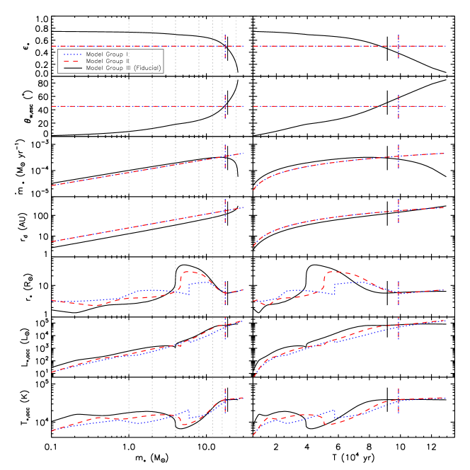
Figure 2.— The evolution of star formation efficiency $\epsilon_{*}$, outflow opening angle $\theta_{w,\mathrm{esc}}$, stellar accretion rate $\dot{m}_{*}$, disk radius $r_{d}$, stellar radius $r_{*}$, stellar + boundary layer accretion luminosity $L_{*,\mathrm{acc}}$, and stellar surface temperature $T_{*,\mathrm{acc}}$ assuming $L_{*,\mathrm{acc}}$ is emitted from the stellar surface as a single black-body. The evolution with both stellar mass (left panels) and time (right panels) are shown. Blue dotted lines are for Model Group I (constant efficiency + MT03 protostellar evolution), red dashed lines are for Model Group II (constant efficiency + Hosokawa evolution), and black solid lines are for Model Group III (varying efficiency + Hosokawa evolution, fiducial). The short vertical lines indicate the moments $m_{*}=M_{\mathrm{env}}$ for each model. The thin vertical dotted lines in the left panels indicate the seven selected evolutionary stages for which we show SEDs and images.

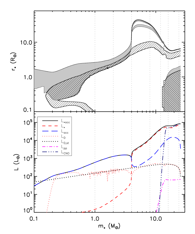
Figure 3.— The protostellar evolution in the fiducial model (Model Group III). Upper panel: evolution of the protostellar radius and internal structure. The shaded region is the convective zone. The region hatched with ‘/’ is the deuterium burning region (where the energy production rate of deuterium burning exceeds 10% of its steady rate), and the region hatched with ‘$\backslash$’ is the hydrogen burning region (where the energy production rate exceeds $0.1L_{*}/m_{*}$). Lower panel: the evolution of different components of the luminosity (stellar luminosity, boundary layer accretion luminosity, and total), and the energy production rates of different nuclear reactions (deuterium burning, pp-chain, CNO-cycle). The steady rate of the deuterium burning (see text) is also shown for reference. The vertical lines are the selected evolutionary stages we perform radiation transfer simulations.

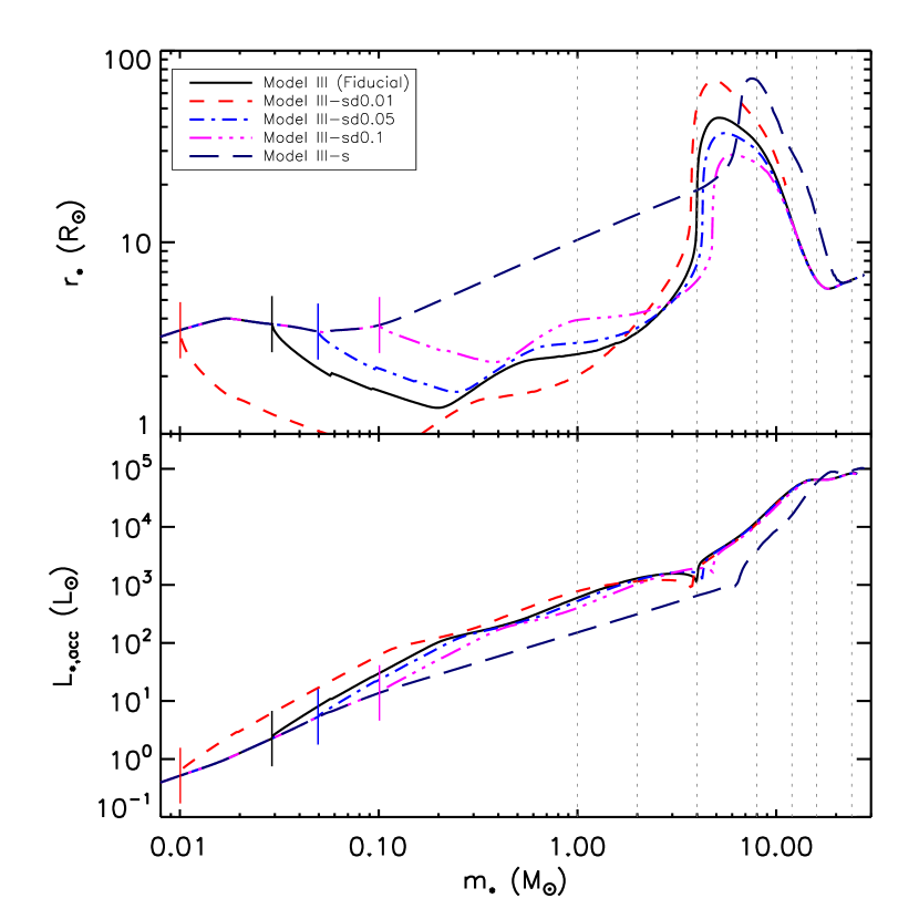
Figure 4.— Evolution of the protostellar radius and total stellar + boundary layer luminosity in models with the cold boundary condition turned on at different stellar masses. The fiducial model (switching to the cold boundary condition at $m_{*}\simeq 0.03M_{\odot}$, see Section 2.2), models with switching points at $m_{*}=0.01M_{\odot}$ (Model III-sd0.01), $m_{*}=0.05M_{\odot}$ (Model III-sd0.05), $m_{*}=0.1M_{\odot}$ (Model III-sd0.1), and a model with hot shock boundary condition all the way to the end (Model III-s) are shown. The short solid vertical bars indicating the switching points. The dotted vertical lines are the seven evolutionary stages that we perform the radiation transfer simulations.

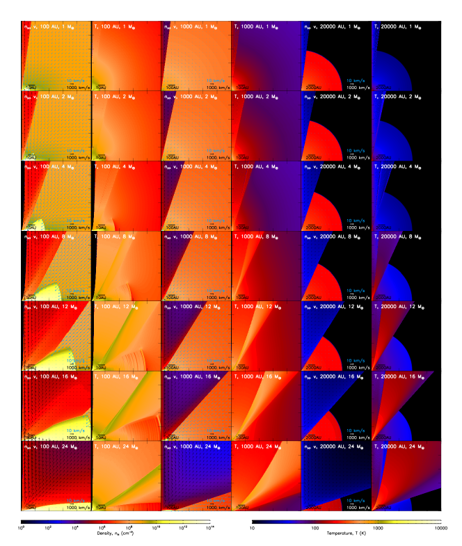
Figure 5.— The input density and converged temperature profiles for the fiducial model ($M_{c}=60M_{\odot}$, $\Sigma_{\rm cl}=1{\rm g}\,{\rm cm}^{-2}$, $\beta_{c}=0.02$) at selected stages with $m_{*}=1$, 2, 4, 8, 12, 16 and 24 $M_{\odot}$. At each stage (each row), these profiles are shown on three different scales (from left to right, 100 AU, 1000 AU and 20000 AU). In each panel, the protostar is at the (0,0) point, the x-axis lies on the disk mid plane and y-axis along the outflow axis. The velocity fields are shown by the arrows. Note that the black arrows for the outflow have a much larger scale than the blue arrows for the infalling envelope.

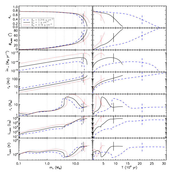
Figure 6.— Same as Figure 2, except comparing models with $M_{c}=60\>M_{\odot}$, $\beta_{c}=0.02$, but different $\Sigma_{\rm cl}$.

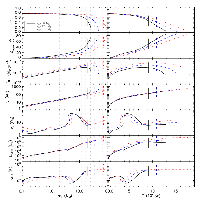
Figure 7.— Same as Figure 2, except comparing models with different initial core masses. All the three models assume an environmental surface density of $\Sigma_{\rm cl}=1\>{\rm g}\,{\rm cm}^{-2}$ and $\beta_{c}=0.02$.

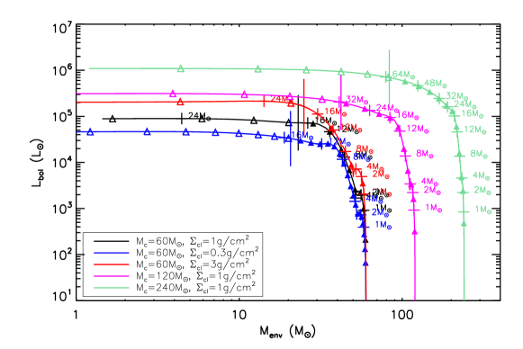
Figure 8.— Evolution of bolometric luminosity with envelope mass in five models with various $M_{c}$ and $\Sigma_{\rm cl}$. The long vertical lines mark the position $m_{*}=M_{\mathrm{env}}$ representing a transition from the accretion phase to the envelope dissipation phase. The triangles mark time intervals of $10^{4}$ yr, with filled triangles in the accretion phase and open triangles in the envelope dissipation phase. The crosses and the numbers mark the stage we select for the RT simulations.

Figure 2 compares the evolution of the star formation efficiencies, the opening angles of the outflow cavities, the stellar accretion rates, the disk sizes, and the protostellar properties of Model Group I (constant efficiency + MT03 protostellar evolution), II (constant efficiency + Hosokawa protostellar evolution), and III (the fiducial model, varying efficiency + Hosokawa protostellar evolution). With the constant efficiency of $\epsilon_{*}=0.5$, Model I and II have a constant opening angle of $\sim 45^{\circ}$, and accretion rate $\dot{m}_{*}=0.5\dot{M}_{*d}$, with $\dot{M}_{*d}$ given by Equation 14. For Model Group III, the instantaneous efficiency $\epsilon_{*}$ decreases as the outflow cavity opens up, and reaches below 0.1 at the end of accretion. At that moment, the stellar mass reaches $\sim 26M_{\odot}$, making the averaged star formation efficiency to be $\bar{\epsilon}_{*f}=26M_{\odot}/60M_{\odot}=0.43$. However, in our model, there is still a disk with mass of $(1/3)m_{*}$ around the star at the end, part of which will continue to accrete on the star, making the final mean star formation efficiency higher than 0.43.

In the figure we also mark the moments when the stellar mass $m_{*}$ equals the envelope mass $M_{\mathrm{env}}=(M_{c}-M_{*d})\cos\theta_{w,\mathrm{esc}}$, representing a transition from the “main accretion phase” during which most of the stellar mass is being accreted to the “clear-up phase” during which the envelope is being dissipated (Andre et al. 2000; Dunham et al. 2014). In the fiducial model, this transition happens at $m_{*}=19\;M_{\odot}$, therefore about 3/4 of the final stellar mass has been accreted at that point. After this point, the outflow opening angle becomes $>50^{\circ}$ and widens quickly, corresponding to the phase that the remnant envelope is being quickly dispersed. This point is also where the accretion rate starts to significantly decline. We also show the evolution with the time, and this transition happens at about $9\times 10^{4}$ yr in the fiducial model (i.e., at about 2/3 of the total formation time). In the other two models with constant efficiencies, such a transition happens at similar stellar mass ($m_{*}=17.6\;M_{\odot}$), but a later time ($\sim 10^{5}$ yr). The “clear-up phase” takes longer in the fiducial model because of the decreasing accretion rate, but not too much longer because the final mass is higher in the cases of constant efficiencies. Note that our selected stages to perform RT simulations mostly cover the main accretion phase except the last stage with $m_{*}=24\;M_{\odot}$. Also these stages cover most of the formation time from $\sim 2.5\times 10^{4}$ yr to $\sim 11\times 10^{4}$ yr in the fiducial model, with longer time spent in the last stage ($m_{*}\sim 24\;M_{\odot}$) than in each earlier stage.

The fourth row of Figure 2 shows the evolution of the disk size in these three models. As discussed in Section 2.1, the disk size is scaled with the collapsed mass $M_{*d}$ as $r_{d}\propto M_{*d}^{2/3}$. The ratio between the stellar mass and the collapsed mass ($m_{*}/M_{*d}$) depends on the history of the star formation efficiency. Since for most of the time except the very late stage, the efficiency is higher in Model Group III, the disks are smaller in Model Group III than in the other two groups at same stellar masses.

The fifth row of Figure 2 compares the evolution of stellar radius in these three cases. All the evolution tracks show similar stages: (1) an early slow contraction stage; (2) a phase in which the radius grows linearly with the mass (linear increase stage) caused by deuterium burning; (3) a slow growth stage (or even slight contraction in the MT03 model) when the D burning is only fed by the accreting material; (4) a fast swelling phase (so called “luminosity wave” stage, Stahler et al. 1986); (5) Kelvin-Helmholz (KH) contraction stage, and (6) the main-sequence stage. Comparing the MT03 model and the Hosokawa model with the same accretion history (i.e. Model Groups I and II), we find the full radial structure protostellar evolution calculation predicts lower protostellar masses at the linear increase stage and the luminosity wave stage, also the maximum radius is larger than that in MT03 model by a factor of 2-3. However, the models predict very similar zero age main sequence (ZAMS) masses. The differences in the protostellar radii between Model Group II and III are mainly due to the higher accretion rate for most of the time in Model Group III, and a lower stellar mass for switching to the cold boundary condition. For Model Group II, we switched to the photospheric boundary condition at $m_{*}=0.1M_{\odot}$, same as the MT03 model; For Model Group III, the outflow first breaks out when $m_{*}\simeq 0.03M_{\odot}$, after which the cold boundary condition is switched on. The last two panels in Figure 2 show the evolution of the (stellar + boundary layer) luminosities and temperatures for these three model groups.

Details of the protostellar evolution in the fiducial model are shown in Figure 3. In the early contraction stage ($m_{*}<0.2M_{\odot}$), because there is no energy production, and also because under the cold boundary condition, the accreting gas carries the same amount of entropy as the gas in the protostellar photosphere, the radius decreases as the mass grows. Deuterium burning begins at $m_{*}\sim 0.2M_{\odot}$ (an initial deuterium abundance of [D/H]=$2.5\times 10^{-5}$ is assumed in our models), after which the radius starts to increase, as the entropy of the star is enhanced by deuterium burning. The deuterium in the inner region is soon consumed, after which the burning is only fed by the deuterium in the accreting gas, therefore the depth of the deuterium burning is limited to the depth of the convective zone. At this stage, the deuterium burning reaches its steady rate

$$L_{\mathrm{D,st}}=\dot{m}_{*}\delta_{\mathrm{D}}=1500L_{\odot}\left(\frac{\dot{m}_{*}}{10^{-3}M_{\odot}\mathrm{yr}^{-1}}\right)\left(\frac{\mathrm{[D/H]}}{2.5\times 10^{-5}}\right),$$ (40)

where $\delta_{\mathrm{D}}$ is the energy available from deuterium burning per unit gas mass. Also in this stage, the produced energy from deuterium burning is absorbed by the outer convective zone, therefore the stellar luminosity is much lower than the total energy production rate, and the luminosity of the system is dominated by the accretion luminosity from the boundary layer ($L_{\mathrm{acc}}$), as shown in the lower panel of Figure 3. As the temperature increases, the opacity gradually becomes lower, the transparent region which is losing energy to outer layers, is moving outward. This propagation of the luminosity is called the “luminosity wave” (Stahler et al. 1986). Especially, at $m_{*}\sim 4M_{\odot}$, most of the interior becomes radiative, and only the outermost layer is absorbing energy from inside and thus experiencing a fast expansion. This dramatic increase in the stellar radius leads to a sudden decrease in the accretion luminosity $L_{\mathrm{acc}}$, and most of the stellar interior becoming radiative makes the stellar luminosity increase significantly and it becomes the dominant luminosity component. The fast swelling phase is followed by Kelvin-Helmholz contraction at $m_{*}\sim 5M_{\odot}$. At $m_{*}\sim 15M_{\odot}$, hydrogen burning starts and the protostar reaches the main-sequence. In the models presented here, the main-sequence luminosity is dominated by the CNO-cycle process of hydrogen burning.

It is also necessary to discuss the possible effects made by different choices of when to switch from the hot shock boundary condition to the cold photospheric boundary condition (see Section 2.2). Figure 4 compares the evolution of the protostellar radii and the luminosities in models with the cold boundary condition turned on at different stellar masses. The protostellar evolution in the case using only hot boundary condition is significantly different than other models with cold boundary condition. Because of the higher entropy brought into the star under the shock boundary condition, the protostellar radius is larger in the early evolution. In such a case, the interior temperature is actually lower, causing later starts of the deuterium burning and the luminosity wave phase. The KH contraction in turn happens later in this case. On the other hand, the evolutions in models with the cold boundary condition are quite similar. With an earlier start of the cold boundary condition, the initial contraction stage starts earlier, leading to an earlier start of deuterium burning. In such a case, the radius before the fast swelling is smaller, but reaches a higher peak at the end of the fast swelling stage. However, the variation in the radius is within a factor of 2 in the mass range that we are interested here. Also they start the luminosity wave stage at similar masses and have very similar evolution profiles from later KH contraction phase to main sequence. Therefore, even though at a certain mass (e.g. $m_{*}=4M_{\odot}$), the stellar radius is strongly affected by the choice on when to switch from hot to cold boundary condition, the general trend will not be affected, as long as we sample enough $m_{*}$ to cover different evolutionary stages.

The input density profiles of the fiducial Model Group III ($M_{c}=60M_{\odot}$, $\Sigma_{\rm cl}=1{\rm g}\,{\rm cm}^{-2}$, and $\beta_{c}=0.02$) are shown in Figure 5. One can clearly see the gradual opening-up of the low-density outflow cavity and the growth of the disk. As in the previous papers, the region outside of the core boundary ($R_{c}$) is assumed to be empty, except that the outflow is followed as far as $5R_{c}$. The possible effects caused by the ambient clump material will be discussed in Section 4.1. The velocity fields of the outflow and the inflow are also shown (note they are on very different scales). The increasing density and velocity of the outflow approaching the axis indicate that the momentum flux is increasing towards the polar direction, as discussed in Section 2.3.

Figure 6 shows the evolution of the protostars and the protostellar cores in three models with same $M_{c}$ but different $\Sigma_{\rm cl}$. Embedded in an environment with a higher $\Sigma_{\rm cl}$, the core is more pressurized and more compact, the accretion rate becomes higher, leading to a higher accretion luminosity. In such a case, although the disk wind is more powerful, it is also harder to sweep up the core material. The combination of these two effects is that the opening angles of the outflow cavities (and therefore the star formation efficiencies) in these three models are very similar in the earlier stages ($m_{*}<8M_{\odot}$), however at later stages, a model with a higher $\Sigma_{\rm cl}$ has a smaller outflow cavity and a higher star formation efficiency, and also reaches a higher final mass. For the protostellar evolution, with a higher $\Sigma_{\rm cl}$ and therefore a higher accretion rate, the deuterium burning, the luminosity wave stage, and the main sequence stage all start at higher stellar masses. In this case, the protostar also becomes much bigger at the end of the luminosity wave stage and in the following KH contraction stage, making the stellar temperature lower while the total luminosity is generally higher. The star formation is much faster in the high surface density environments. The formation time is $t_{f}\propto M_{c}^{1/4}\Sigma_{\rm cl}^{-3/4}$ (MT03). And we also see that the fraction of time spent in the main accretion phase tends to increase with higher $\Sigma_{\rm cl}$.

Figure 7 compares the evolution in models with different $M_{c}$ but with same $\Sigma_{\rm cl}$. The evolution of the star formation efficiencies, the outflow cavity opening angles, the accretion rates and the disk sizes with the stellar mass are very different in these three models as expected, since they are strongly affected by the mass of the core and therefore more dependent on parameters such as $m_{*}/M_{c}$. On the other hand, the evolution of the protostellar properties with stellar mass are very similar, especially the stellar + boundary layer accretion luminosity seems to only depend on the stellar mass. Due to the different accretion rates, the protostellar radius and the beginning of the luminosity wave stage and the main sequence stage are affected by $M_{c}$, but not as strongly as by $\Sigma_{\rm cl}$, since the accretion rate is more affected by the environmental surface density (the accretion rate $\dot{m}_{*}\propto M_{c}^{1/2}\Sigma_{\rm cl}^{3/4}$, see Equation 14). In Table 1, we list the stellar masses of the luminosity wave stages $m_{*,\mathrm{lw}}$, the ZAMS masses $m_{*,\mathrm{ZAMS}}$ (defined as the stellar mass when the total energy production rate from hydrogen burning exceeds 80% of the stellar luminosity), the final stellar masses $m_{*f}$, and the mean star formation efficiencies $\bar{\epsilon}_{*f}=m_{*f}/M_{c}$ of these models with different initial conditions. Although the explored parameter space is relatively limited here, we can still see a trend that a higher $\bar{\epsilon}_{*f}$ is achieved with a higher $\Sigma_{\rm cl}$.

Figure 8 shows how the different models evolve on the $L_{\mathrm{bol}}-M_{\mathrm{env}}$ diagram. Such diagrams are used to identify the evolutionary stages of protostars (Molinari et al. 2008). Indeed, we see such evolution of the model tracks on this diagram. Especially, sources in the main accretion phase can be recognized in the lower-right part of this diagram and the sources in the envelope clear-up phase generally occupy the upper-left region of the diagram, with the division running diagonally through the turning points of each evolutionary track. However, one needs to be cautious when comparing this diagram with observations. First, only the core mass is included here, while in real observations, additional clump material will usually be included due to low resolutions in single-dish FIR observations, which will cause the tracks to move to the right. So careful subtraction of the clump material needs to be made in order to compare the observation to the models. Second, as we will show below, because more radiation from the protostar is emitted in polar directions due to the anisotropic envelope, the integrated bolometric luminosity from SEDs can be different by an order of magnitude or more depending on the inclination. This may cause significant confusion especially for the sources around the turning points of the evolutionary tracks.

Table 1Protostellar evolution in models with different initial conditions

$M_{c}$ ($M_{\odot}$)	$\Sigma_{\rm cl}$ (${\rm g}\,{\rm cm}^{-2}$)	$m_{*,\mathrm{lw}}$ ($M_{\odot}$)	$m_{*,\mathrm{ZAMS}}$ ($M_{\odot}$)	$m_{*f}$ ($M_{\odot}$)	$\bar{\epsilon}_{*f}$
60	1	4.0	14.2	25.6	0.43
60	0.3	3.3	10.7	20.5	0.34
60	3	4.9	18.3	31.4	0.52
120	1	4.5	15.1	46.0	0.38
240	1	5.3	16.0	90.1	0.37

3.2. Evolution of the Temperature Structure of the Envelope

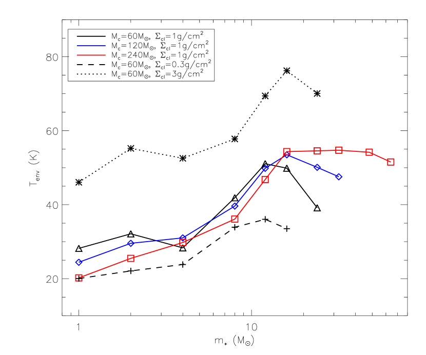
Figure 9.— The evolution of the mass weighted mean temperature in the envelope with the growth of the protostar.

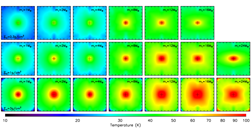
Figure 10.— The projected mass-weighted temperature map for models with $M_{c}=60\;M_{\odot}$ and $\Sigma_{\rm cl}=0.3$, 1 and 3 ${\rm g}\,{\rm cm}^{-2}$ (from top to bottom) at selected stages. The source is viewed at a distance of 1 kpc and an inclination of 60^∘ between the line of sight and the outflow axis. Each panel is $10\arcsec\times 10\arcsec$ ($1\times 10^{4}$ AU) and convolved with a 1$\arcsec$ beam.

The temperature structures of each evolutionary stage in the fiducial model are shown in Figure 5. As the protostar grows, due to the increase of the luminosity, the envelope is gradually heated up. We assumed that if the streamline of the outflow originates from the outer dusty disk (with temperature at surface lower than 1400 K), then the wind is dusty too. The dusty and dust-free regions of the outflow can be seen in the temperature profiles as the dusty part can be heated more easily and is thus warmer. The dusty wind does not appear in the early stages because the outflow cavity and the disk are both small, so all the streamlines come from the inner hot dust-free disk region. But in the later stages ($m_{*}=8$, 12, 16, 24 $M_{\odot}$), the fraction (volume and mass) of the outflow cavity which is dusty gradually becomes larger. Whether this dusty outflow exists or not (e.g., we are ignoring possible destruction of dust by internal shocks in the outflow) also affects the temperature of the envelope and certainly affects the infrared appearance of the outflow cavities.

Figure 9 shows how the mass-weighted mean temperature of the envelope evolves with stellar mass for models with different $M_{c}$ and $\Sigma_{\rm cl}$. No external heating is included. The envelope temperature is affected by several factors. The first is the luminosity, which increases as the protostar grows. All the models show a general trend that the temperature increases with the protostellar mass. For the fiducial model, the envelope is heated from $\sim$ 30 K in the earliest stage up to $\sim$ 60 K in the later stages. This factor is also strongly affecting the envelope temperatures with different $\Sigma_{\rm cl}$, since the core with a higher $\Sigma_{\rm cl}$ has a higher accretion rate and luminosity. In the model with $\Sigma_{\rm cl}=3\>{\rm g}\,{\rm cm}^{-2}$, the envelope in the late stages is heated to close 80 K, $\sim 50$ K higher than the temperature in the model with $\Sigma_{\rm cl}=0.3\>{\rm g}\,{\rm cm}^{-2}$. On the other hand, the envelope temperature is not so dependent on the initial core mass $M_{c}$, since the luminosity evolution appears very similar in models with different $M_{c}$ but the same $\Sigma_{\rm cl}$. The second factor is the size of the envelope. A bigger envelope will have more cold material in the outer region, leading to a lower mean temperature, as shown by comparing the models with the same $\Sigma_{\rm cl}$ but different $M_{c}$ in their early stages. The third factor is the opening angle of the outflow cavity. Especially, in the final stage, the outflow cavity is very wide, so that the residual envelope in the low latitude is harder to be heated by the stellar radiation because of the shielding from the disk and the dusty outflow. This explains the decrease of the envelope temperature in the latest stages in all of the five models. The higher envelope temperatures in the late stages in the model with higher $M_{c}$ are also caused by the smaller outflow cavity. Fourth, the stellar temperature may also have an effect. The drop or slow increase in the envelope temperature at $m_{*}\sim 4M_{\odot}$ may be caused by the sudden decrease of the protostellar temperature during the fast swelling phase. These models predict that, even in the low $\Sigma_{\rm cl}=0.3\>{\rm g\>cm^{-2}}$ case, the envelope temperature quickly reaches $\sim 20$ K, which has implications for CO freeze-out and deuteration of particular species such as $\rm N_{2}H^{+}$ (Fontani et al. 2011; Tan et al. 2014).

Figure 10 shows the projected mass-weighted temperature maps at different stages for the three models with different $\Sigma_{\rm cl}$ but same $M_{c}$. The evolution of the thermal structure of the envelope as the protostar grows can be clearly seen. The profiles are mostly spherically symmetric except at later stages when they are affected by the well-developed wide-angle outflow cavity (they appear elongated or even rectangular, perpendicular to the outflow axis). As discussed above, the envelope generally is warmer in the higher $\Sigma_{\rm cl}$ environment. Also, the warmest phase does not happen at the latest stage, because of the development of the outflow cavity. Such profiles can be compared with the observed temperature maps around massive protostars using temperature-sensitive molecular tracers (e.g., Brogan et al. 2011).

3.3. Spectral Energy Distributions

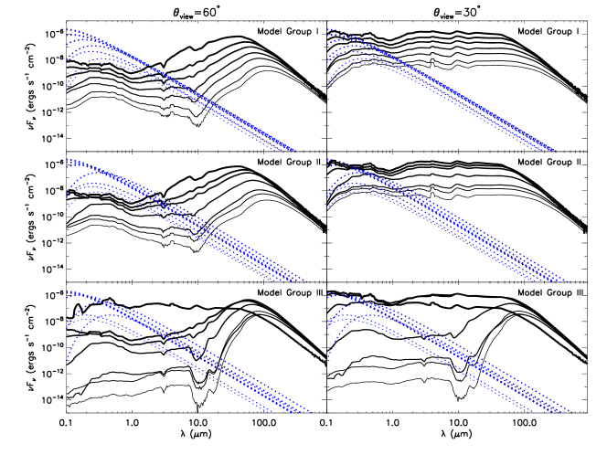
Figure 11.— Evolution of the SEDs in Model Group I, II and III (from top to bottom) at inclinations of $60^{\circ}$ (left) and $30^{\circ}$ (right) between the line of sight and the axis. A distance of 1 kpc is assumed. In each panel, the SEDs of seven evolutionary stages are shown (from thin to thick lines: $m_{*}$ = 1, 2, 4, 8, 12, 16, and 24 $M_{\odot}$). The blue dotted lines are the input stellar spectra including the stellar luminosity and the boundary layer accretion luminosity as a single black body.

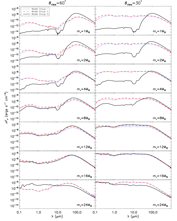
Figure 12.— A comparison of SEDs of Model I, II, and III (the fiducial model) at the seven evolutionary stages (from top to bottom: $m_{*}$ = 1, 2, 4, 8, 12, 16, and 24 $M_{\odot}$) at inclinations of $60^{\circ}$ (left) and $30^{\circ}$ (right) between the line of sight and the axis. A distance of 1 kpc is assumed.

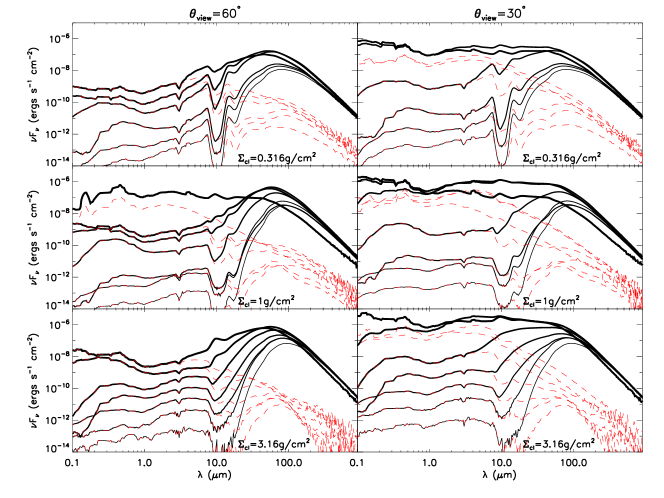
Figure 13.— Evolution of the SEDs in the models with same initial core mass $M_{c}=60\;M_{\odot}$ but different environmental surface densities ($\Sigma_{\rm cl}=0.3$, 1 and 3 ${\rm g}\,{\rm cm}^{-2}$ from top to bottom). In each panel the SEDs of 6 evolutionary stages are shown (from thin to thick lines: $m_{*}$ = 1, 2, 4, 8, 12, 16, and 24 $M_{\odot}$), except in the case with $\Sigma_{\rm cl}=0.3\>{\rm g}\,{\rm cm}^{-2}$ the final stellar mass has not reached $24M_{\odot}$. The red dashed lines are the scattered light only. A distance of 1 kpc is assumed and SEDs at two inclination angles are shown.

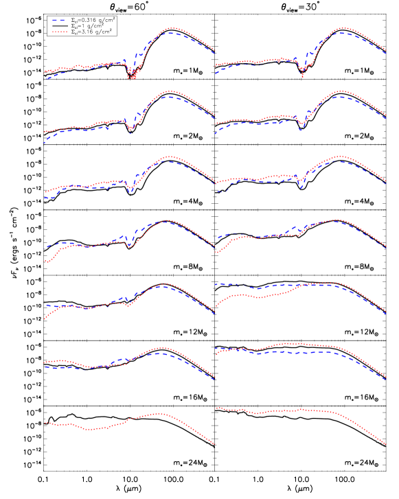
Figure 14.— A comparison of SEDs of models with three different $\Sigma_{\rm cl}$ at the six evolutionary stages (from top to bottom: $m_{*}$ = 1, 2, 4, 8, 12, 16, and 24 $M_{\odot}$) at inclinations of $60^{\circ}$ (left) and $30^{\circ}$ (right) between the line of sight and the axis. A distance of 1 kpc is assumed. Note in the case with $\Sigma_{\rm cl}=0.3\>{\rm g}\,{\rm cm}^{-2}$ the final stellar mass has not reached $24M_{\odot}$).

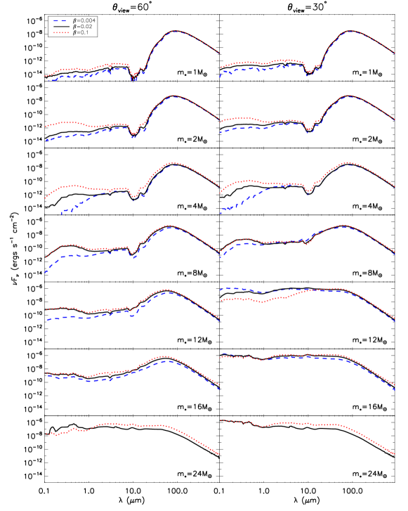
Figure 15.— A comparison of SEDs of models with three different disk sizes at the seven evolutionary stages (from top to bottom: $m_{*}$ = 1, 2, 4, 8, 12, 16, and 24 $M_{\odot}$) at inclinations of $60^{\circ}$ (left) and $30^{\circ}$ (right) between the line of sight and the axis. A distance of 1 kpc is assumed. The SEDs in black are for the fiducial model with $\beta_{c}=0.02$. The blue and red are for models with $\beta_{c}=0.004$ and 0.1, i.e. with disk sizes 5 times smaller or larger than the fiducial model respectively.

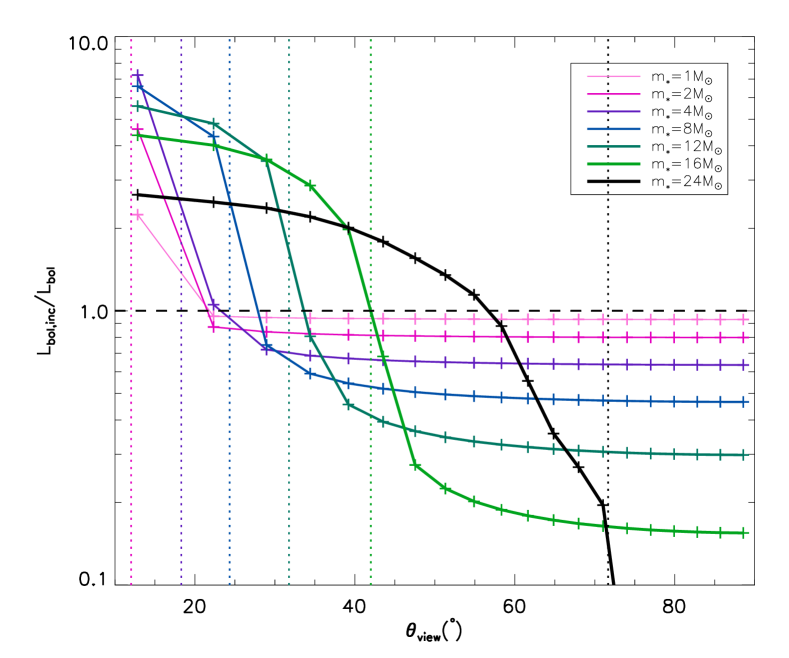
Figure 16.— The inferred bolometric luminosities at different viewing angles scaled by the true bolometric luminosities for the fiducial model. Seven evolutionary stages are shown in different colors. For each stage, inferred luminosities at 20 inclinations evenly sampled in the cosine space are shown, and the opening angle of the outflow cavity at that stage is also marked by a vertical dotted line in the same color.

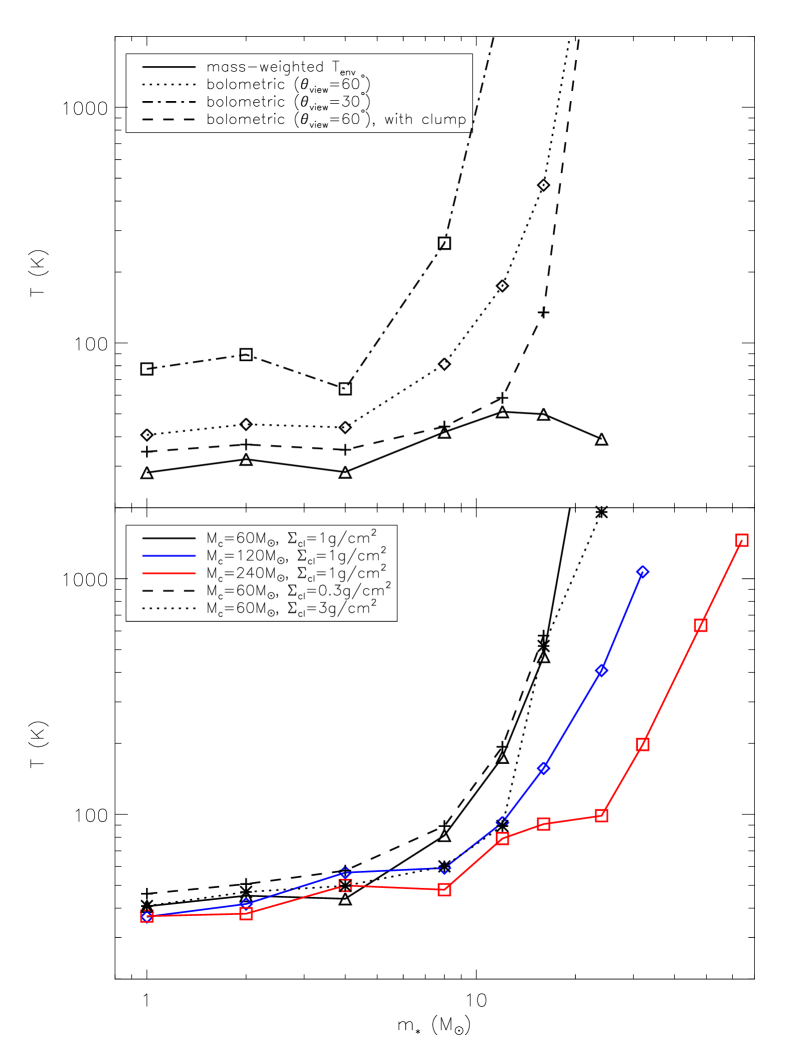
Figure 17.— The evolution of the bolometric temperature of the massive young stellar objects. In the upper panel, we show the evolutions of bolometric luminosity in the fiducial model at inclinations of $60^{\circ}$ and $30^{\circ}$. A model with additional ambient clump material included is also shown. The mass-weighted envelope temperature (from Figure 9) is also shown for reference. In the lower panel, we show the bolometric luminosities of five models with different $M_{c}$ and $\Sigma_{\rm cl}$ at inclination of $60^{\circ}$.

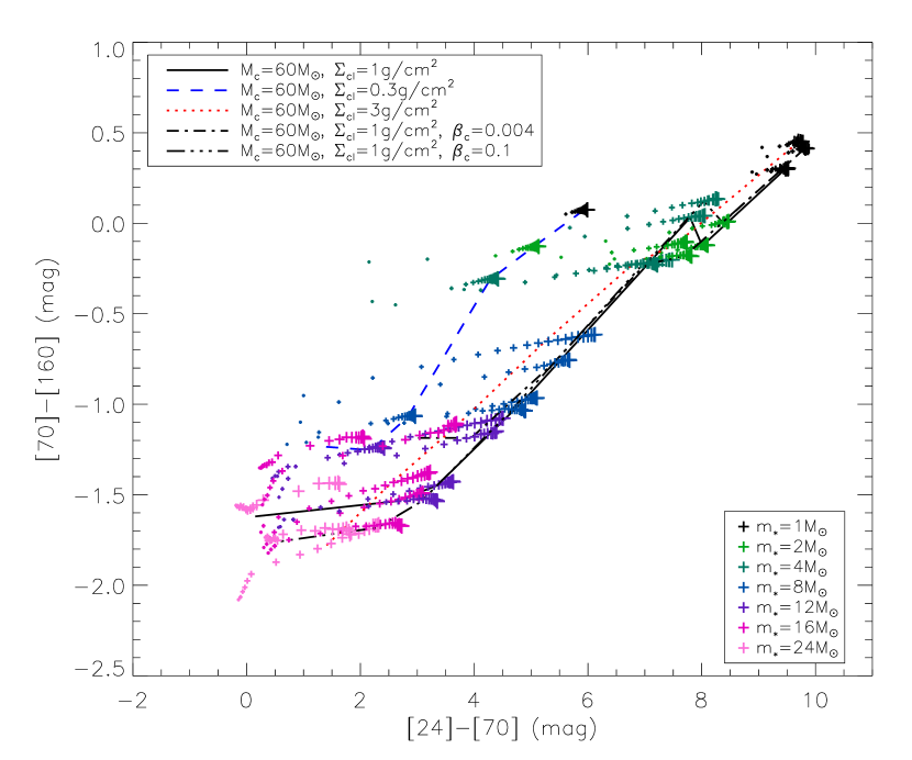
Figure 18.— The color-color diagram of the fiducial model, the models with high and low $\Sigma_{\rm cl}$, and the models with larger and smaller disk sizes. Groups of data points linked by different line types represent the five evolutionary tracks. At each stages, data points of 20 inclinations evenly sampled in the cosine space are shown (from small to large are from face-on to edge-on). The data points with the same protostellar masses are in the same colors.

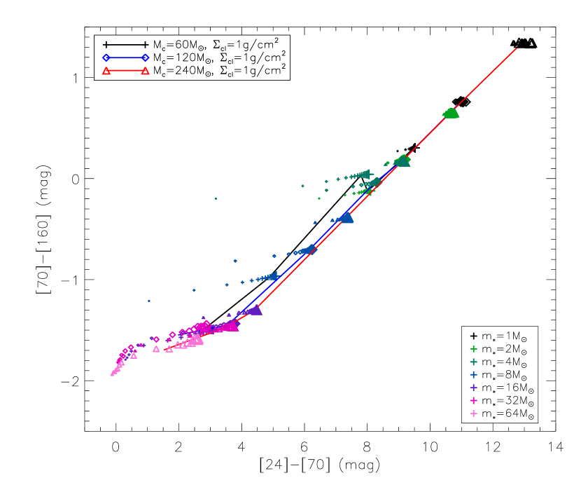
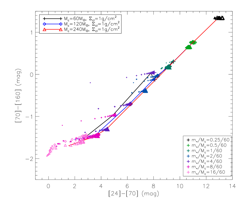
Figure 19.— Upper: The color-color diagram of three models with different initial core masses. Each line linking data points of same symbol represent an evolutionary track. The colors of the data points represent the protostellar masses. The size of the labels represents the inclination same as in Figure 18. Lower: Same as the upper panel, but the colors of the labels represent protostellar masses scaled by the initial core masses $m_{*}/M_{c}$.

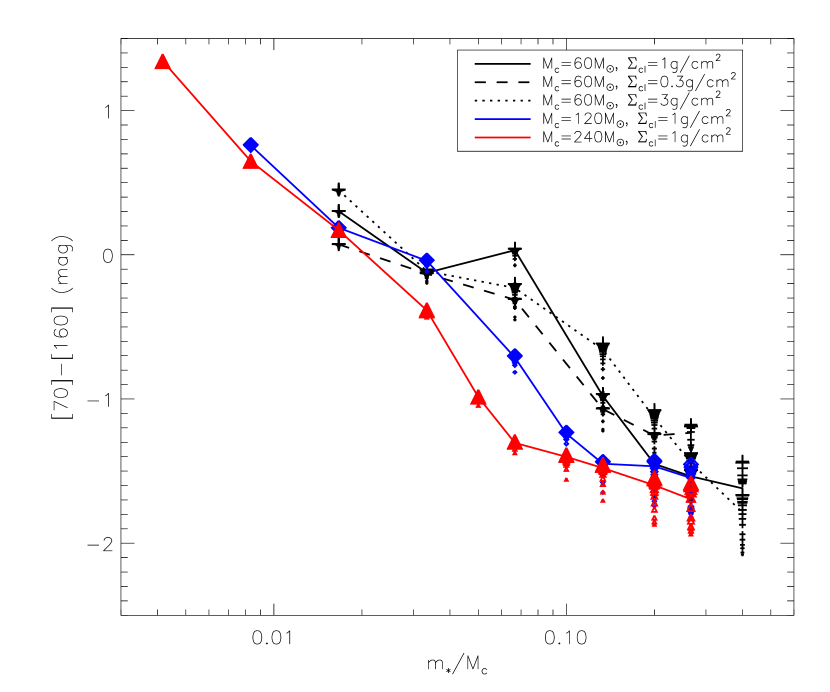
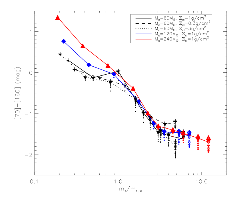
Figure 20.— Upper: evolution of the [70 $\mu$m]-[160 $\mu$m] color with the protostellar mass scaled by the initial core masses. Lower: Same as the upper panel, but with the protostellar mass scaled by the mass at the luminosity wave stage ($m_{*,\mathrm{lw}}$). In each panel, five evolutionary tracks with various initial conditions are shown, with the data points showing the colors of 20 inclinations at each of the selected stages

Figure 11 shows how the SEDs evolve in Model Groups I, II and III. All these three model groups show similar trends. As the protostar grows, fluxes at wavelengths shorter than $\sim 100\mu$m increase and the far-IR peaks become higher and move to shorter wavelengths. In the most evolved stage, this peak reaches $\sim 40\mu$m. While the slopes of the SEDs in the sub-mm and at wavelengths shorter than 10 $\mu$m are less affected by the evolution, the SED from 10 $\mu$m to 100 $\mu$m becomes less steep. Therefore, the color of the bands at these wavelengths may be used as an indicator of the evolutionary sequence (see Section 3.4 below). The 10 $\mu$m silicate feature is also becoming less deep as the protostar evolves. A flat SED from near-IR to far-IR only appears when the line of sight is passing through the outflow cavity ($30^{\circ}$ inclination in Model I, II, and the last stage of Model III at both inclinations), which can be used as an indicator of a near face-on source. Despite the similar general trend, the differences made by the gradual opening-up of the outflow are significant. In Model Group III, as the initial opening angle of the outflow cavity is very small, the fluxes in the shorter wavelengths start from a much lower level and are increasing faster with time than in the other two model groups. The 10 $\mu$m to 40 $\mu$m slope is also changing more dramatically. This emphasizes the importance of including a realistic efficiency history to model observed SEDs.

Detailed comparison among these three model groups at each stage are shown in Figure 12. The SEDs of Model Groups I and II are very similar, since they have same evolutionary histories of the outflow opening angle, formation efficiency, and accretion rate. The only differences are caused the higher luminosity in Model Group II (see the sixth panel of Figure 2). In the early stages ($m_{*}=1$, 2 $M_{\odot}$), this is because of the smaller radius leading to a higher accretion luminosity; in later stages ($m_{*}=8$, 12 $M_{\odot}$), this is because of the higher stellar luminosity reached in Model Group II. Although the accretion history is same in Model Groups I and II, the earlier start of deuterium burning in Model Group II produces more energy which is being radiated from the protostar in the KH contraction stage. But these appear to be minor effects compared to that caused by different histories of formation efficiency and the opening angle of the outflow cavity. With the outflow cavity evolving self-consistently, Model Group III starts with a small outflow cavity, making the fluxes at short wavelengths much lower and the far-IR peak much higher at the beginning. After the outflow cavity gradually opens up, the SED becomes similar to those of Model Groups I and II.

Figure 13 compares the evolution of the SEDs of the fiducial model and its two variants with higher and lower $\Sigma_{\rm cl}$. The red curves show the scattered light only. As long as the line of sight passes through the envelope, the fluxes at short wavelengths are scattering dominated. But the wavelength at which the emission starts to dominate depends on the evolutionary stage and the mass surface density. For the most embedded cases, scattering dominates up to $\gtrsim 10\mu$m, while in the most evolved cases, the direct emission starts to dominate at $\sim 3\mu$m. Detailed comparison among these three models at each stage is shown in Figure 14.

The differences in the SEDs are caused by several factors. First, at any given stage, the luminosity increases with $\Sigma_{\rm cl}$ (see the sixth panel of Figure 6). In the earlier stages ($m_{*}\lesssim 4M_{\odot}$), this is because of the higher accretion rate with a higher $\Sigma_{\rm cl}$; in later stages ($m_{*}\gtrsim 12M_{\odot}$), this is caused by the higher stellar luminosity in the case of a higher $\Sigma_{\rm cl}$. Especially the far-IR peak is affected by the total luminosity. Second, the mid-IR fluxes are affected by the extinction of the envelope which is lower in the low $\Sigma_{\rm cl}$ case, causing the mid-IR fluxes in such a model to be often higher than in the other two cases at the same inclination angle. Third, the evolution of the protostellar radius after the luminosity wave stage (e.g., $m_{*}=4$, 8 , 12 $M_{\odot}$) is very different depending on $\Sigma_{\rm cl}$, affecting the stellar surface temperature and the input stellar spectrum, which causes differences in the short wavelength SEDs in these stages. Fourth, the outflow cavity is developing faster in the lower $\Sigma_{\rm cl}$ case since the core is less dense and it is easier for the outflow to sweep up the core material. This affects the SED in the later stages. For example, at $m_{*}=24M_{\odot}$, the line of sight with an inclination of $60^{\circ}$ passes through the outflow cavity in the model with $\Sigma_{\rm cl}=1\>{\rm g}\,{\rm cm}^{-2}$, but still passes through the envelope in the model with higher $\Sigma_{\rm cl}$, which causes the differences on the SEDs shown in the left-bottom panel.

Figure 15 compares the SEDs of the fiducial model and its two variants with different disk sizes. As discussed in Section 2.1, the models with $\beta_{c}=0.1$ have disks five times larger than the fiducial model with $\beta_{c}=0.02$, which also makes the disks thiner and less dense. The opposite is true for the model with $\beta_{c}=0.004$. In most of the cases, the fluxes are higher with larger disks, which may be caused by the fact that with a larger disk, the outflow cavity is wider at the base, a larger fraction of the outflow is launched from the outer dusty disk and becomes dusty according to our assumption, leading to a warm dusty region around the disk at the base of the outflow. Also with a thiner disk the radiation from the protostar is less shielded. This difference can be seen at wavelengths $<20\;\mu$m in earlier stages, and gradually is seen in the FIR when the outflow opening angle becomes larger and the disk becomes more exposed. The significant differences at wavelengths $<1\>\mu$m at $m_{*}=2-12\;M_{\odot}$ are caused by the different evolution of the protostellar radius in these three models around these stages. To sum up, the SED at wavelengths $>1\>\mu$m is not so sensitive to a factor of 25 variation in disk size.

Due to the existence of the low-density outflow cavity, the extinction varies with the inclination of the viewing angle, and more radiation is escaping from the polar direction, which is known as the “flashlight effect” (Nakano et al. 1995;Yorke & Bodenheimer 1999). This causes the bolometric luminosity integrated from an observed SED to be larger or lower than the true bolometric luminosity of the source by a factor up to several depending on whether the source is face-on or edge-on. Figure 16 shows this flashlight effect at different evolutionary stages in the fiducial model. Here, 20 inclinations evenly distributed in cosine (i.e. with equal probability to be observed in such an angle) are shown. At early stages, as the outflow cavity is still small, over most of the range of inclinations the inferred directed bolometric luminosity is close to the true total luminosity; the exception is if the source is seen at a nearly face-on view ($\lesssim 20^{\circ}$). The flashlight effect becomes stronger in the later stages when a wider outflow cavity ($>20^{\circ}$) has developed. In these cases, from face-on view to edge-on view, the inferred luminosity varies from higher than the true bolometric luminosity by a factor of $\sim 3-5$ to lower by a factor of $\sim 2-5$. Due to this factor, caution needs to be taken when using the observed total luminosity to infer the mass of a massive protostar. For example, including possible flashlight effect, Zhang et al. (2013b) estimate the total luminosity of the massive protostar G35.2-0.74N to be larger than the directly inferred luminosity by a factor of 2 - 6, leading to a protostellar mass significantly higher than some previously inferred values.

From the SEDs, we can also calculate the bolometric temperature, which is defined as (citealt[]ML93)

$$T_{\mathrm{bol}}\equiv 1.25\times 10^{-11}\langle\nu\rangle\;\rm{K\;Hz}^{-1},$$ (41)

where $\langle\nu\rangle\equiv\int^{\infty}_{0}\nu F_{\nu}d\nu/\int^{\infty}_{0}F_{\nu}d\nu$ is the flux weighted mean frequency. With such a definition, one can expect that $T_{\mathrm{bol}}$ will rise as a YSO evolves and the envelope is dispersed. Therefore, the bolometric temperature is useful as an indicator of evolutionary sequence, rather than representing the thermal conditions of the envelope. As shown in the upper panel of Figure 17, $T_{\mathrm{bol}}$ is generally higher than the mass weighted envelope temperature even in the early stages when the cold FIR emitting envelope dominates the SED. Then $T_{\mathrm{bol}}$ rises dramatically in the later stages up to $>1000$ K. Since $T_{\mathrm{bol}}$ is derived from the SED, we also expect it is highly dependent on the inclination, and affected by the ambient clump material (see Section 4.1). Indeed, from Figure 17, we see that $T_{\mathrm{bol}}$ is much higher in a more face-on view. Also the bolometric luminosity is lower when including the ambient clump material, which provides additional extinction and cold FIR emitting material. In Figure 17, we also show the evolution of $T_{\mathrm{bol}}$ in five models with different $M_{c}$ and $\Sigma_{\rm cl}$. They all start from $\sim$40 to 50 K and rapidly increase to $>100$ K as the outflow cavity widens. In the later stages, at the same $m_{*}$, the outflow opening angle is much smaller in a model with higher $M_{c}$ causing the difference in $T_{\mathrm{bol}}$ between the models with different $M_{c}$.

3.4. Color-color Diagrams

The evolutionary stages of protostars are usually identified from the shape of the SED, e.g., colors or slope index at certain wavelength range. The deeply embedded early phase usually shows high far-IR fluxes but little mid-IR or near-IR fluxes. The short wavelength fluxes increase as the source evolves to later stage. However there are degeneracies caused by inclination, for example, at an edge-on view the fluxes in the near- and mid-IR are much lower than those at a face-on view, mimicking the SED of an early stage protostar. Different core properties such as their masses and mass surface densities may also introduce additional scatter. In this section, we study if we can tell the evolutionary sequences from the observed colors of the sources, in spite of different inclinations, surface densities and initial core masses.

Figure 18 shows a color-color diagram of the fiducial model, along with the two models with higher and lower $\Sigma_{\rm cl}$, and another two models with different disk sizes. Here the color [X $\mu$m]-[Y $\mu$m] is simply defined as $-2.5\lg[F_{\nu}(\mathrm{X}\>\mu\mathrm{m})/F_{\nu}(\mathrm{Y}\>\mu\mathrm{m})]$. For each model at each evolutionary stage, data points of 20 inclinations evenly sampled in the cosine space are shown. Fluxes at wavelengths longer than 24 $\mu$m are used to minimize the scatter caused by the inclination. In these bands, the colors appear to be less dependent on the inclinations. Most of the data points of different inclinations are clustered together on the diagram except in the later stages when the outflow cavity becomes quite wide. At earlier stages, data points of low inclinations show some scatter on [24 $\mu$m]-[70 $\mu$m] color. But for each model, the evolutionary stages are clearly distinguishable in such a diagram. The colors are not so affected by the disk sizes. But significant scatter can be caused by the different surface densities of the star-forming environments. Especially, compared to the fiducial models, the model with lower $\Sigma_{\rm cl}$ has a significant shift in the [24 $\mu$m]-[70 $\mu$m] colors. However, despite the scatter, the general trend of the colors with the evolution of the protostars is still obvious.

The colors for the models with different initial core masses are shown in the upper panel of Figure 19. The evolutionary tracks of these three models lie close together, indicating that, among the three initial conditions ($M_{c}$, $\Sigma_{\rm cl}$, $\beta_{c}$) we explore here, the location of a evolutionary track on such a color-color diagram is only strongly dependent on the environmental surface density $\Sigma_{\rm cl}$. Similar to Figure 18, a general dependence of the colors on the evolutionary stage is evident. However, given a position on such a color-color diagram, it is difficult to find the particular protostellar mass. Especially, in the early stages ($m_{*}\lesssim 4\>M_{\odot}$) and the late stages ($m_{*}\gtrsim 16\>M_{\odot}$), the points of different $m_{*}$ overlap with each other. Instead of the protostellar mass, the scaled protostellar mass by the initial core mass ($m_{*}/M_{c}$) may be a better indicator of the evolutionary stage, since the evolution of the outflow cavity is more dependent on $m_{*}/M_{c}$ than $m_{*}$, and the opening angle of the outflow cavity significantly affects the SEDs and the colors. As the lower panel of Figure 19 shows, the scatter on the color-color diagram is significantly improved with this scaled protostellar mass, especially in the early stages. This can be seen more clearly in the upper panel of Figure 20, where we show the evolution of the [70 $\mu$m]-[160 $\mu$m] color with the scaled protostellar mass ($m_{*}/M_{c}$) in five models with different $M_{c}$ and $\Sigma_{\rm cl}$. The scatter is large for the intermediate stage. This is caused by the different protostellar evolution histories in these models. The scatter at the middle stages becomes much smaller if we scale the protostellar mass by the protostellar mass at the luminosity wave stage $m_{*,\mathrm{lw}}$, as shown in the lower panel of Figure 20. This implies that after the protostar reaches its luminosity wave stage, the sudden increase of the stellar radius and the corresponding decrease of the stellar surface temperature cause significant change of the colors even in the far-IR bands. On a color-color diagram such as Figure 19, before the protostar reaches the luminosity wave stage, a source appears on the upper-right region, and moves to the lower-left region in the luminosity wave stage and the following KH contraction stages. If the accretion rate increases with time (except at very late stage) as the Turbulent Core model predicts, this transition on the color-color diagram can be fast compared to the duration of the early and late stages, therefore a large sample of massive protostars may appear as two groups on such a color-color diagram, as indicated by some studies of large sample of massive protostars (Molinari et al. 2008).

These results indicate that the color-color diagram can be very useful to determine the evolutionary stages of a massive protostar, although there is scatter caused by the environmental surface density and the initial mass of the core. The scatter due to the inclination can be minimized by using the colors at longer wavelengths. At early and late stages, the color seems to be more dependent on the time frame of star formation ($m_{*}/M_{c}$), while in the middle stages, the color seems to indicate the relative stage of protostellar evolution. However, additional scatter may be introduced in by possible binarity, or the uncertainty of the ambient clump environment.

3.5. Images

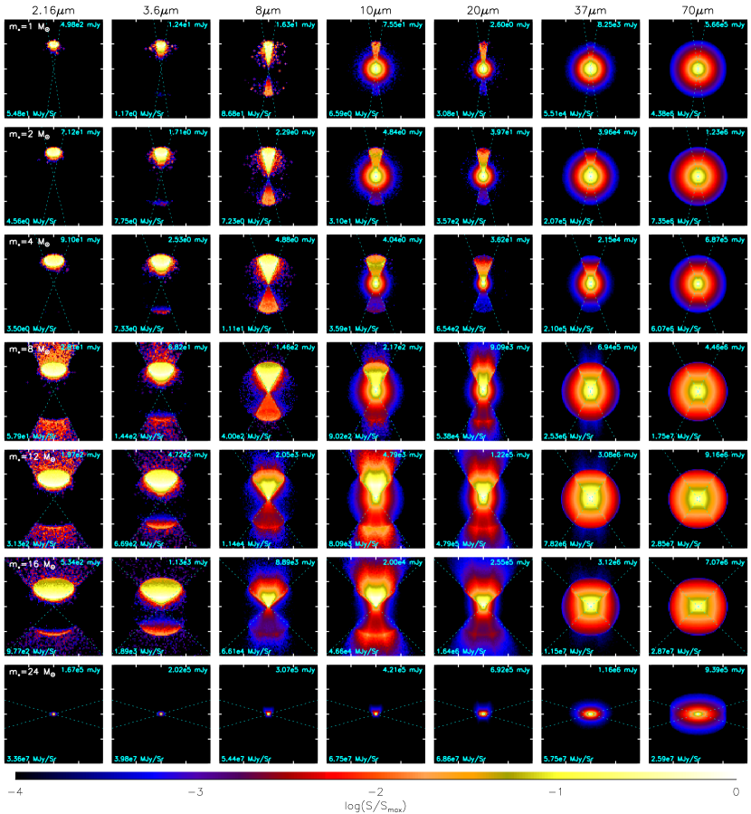
Figure 21.— Resolved images for the selected evolutionary stages ($m_{*}=1$, 2, 4, 8, 12, 16, and 24 $M_{\odot}$ from top to bottom) of the fiducial model in various bands (columns) at the inclination of $60^{\circ}$ between the line of sight and the axis. Each image is normalized to its maximum surface brightness, which is labeled in the lower-left corner. The total fluxes are labeled in the upper-right corners. A distance of 1 kpc is assumed. Each image has a field of view of $40\arcsec\times 40\arcsec$. The dotted lines mark the projected opening angle of the outflow cavity on the sky plane.

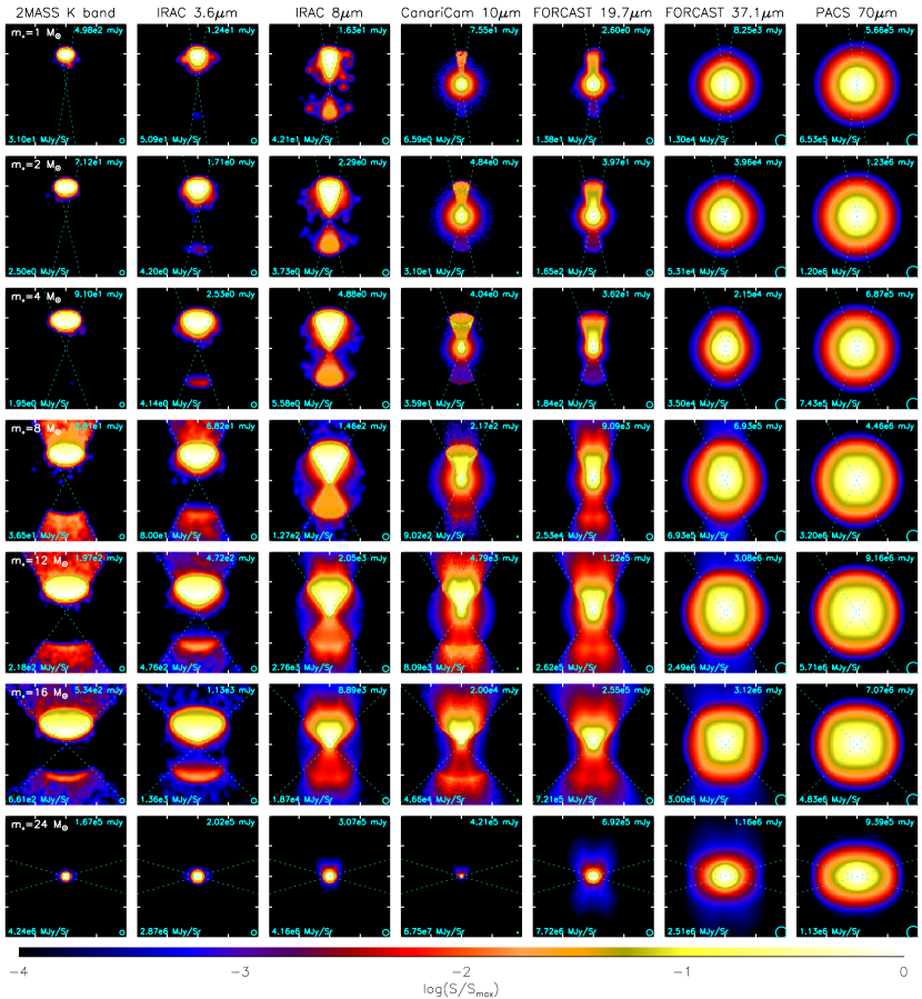
Figure 22.— Same as Figure 21, except convolved with the beam of each instrument which is shown as a circle of diameter equal to the full-width at half-maximum on the bottom-right corner.

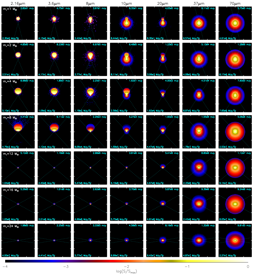
Figure 23.— Same as Figure 21, except at an inclination of $30^{\circ}$.

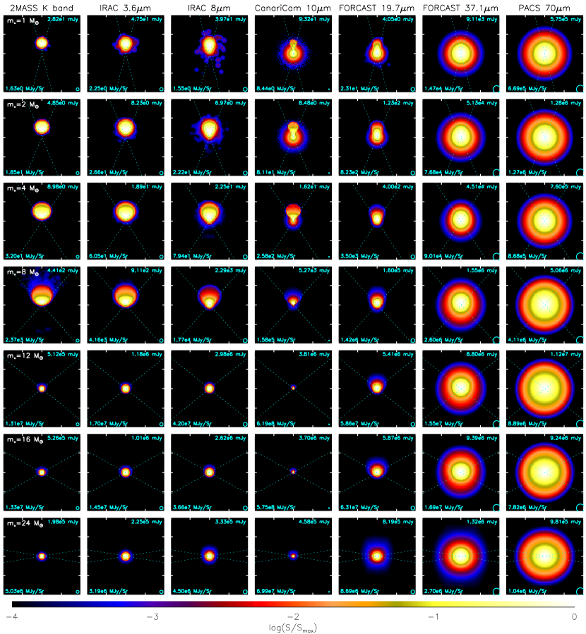
Figure 24.— Same as Figure 22, except at an inclination of $30^{\circ}$.

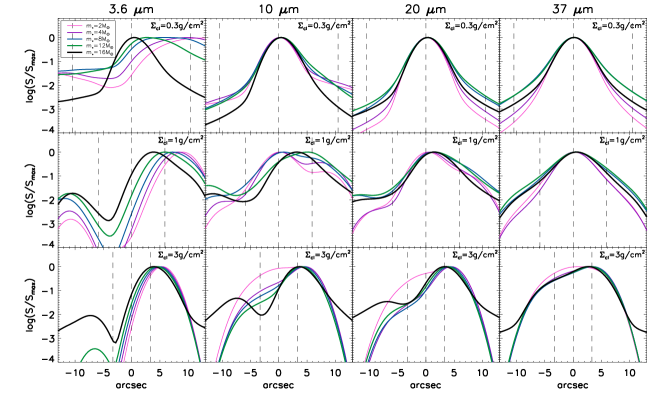
Figure 25.— Intensity distribution along the projected outflow axis at an inclination of $60^{\circ}$. The intensities are convolved with a beam of FWHM of 4$\arcsec$ and normalized by their maximum. Profiles at four wavelengths (columns) for models with different environmental surface densities (rows) are shown. In each panel, the curves in different colors and width show the evolution of the intensity profile with the growth of the protostar. The vertical lines mark the offsets of $-R_{c}/2$ (far-facing outflow), 0, and $R_{c}/2$ (near-facing outflow) to the center on the projected outflow axis.

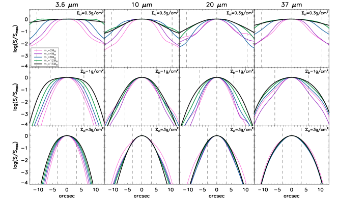
Figure 26.— Intensity distribution along a strip crossing the core and perpendicular to the axis, with an offset to the center of $R_{c}/2$ (the facing outflow), at an inclination of $60^{\circ}$. The intensities are convolved with a beam of FWHM of 4$\arcsec$ and normalized by the values on the axis. Profiles at four wavelengths (columns) for models with different environmental surface densities (rows) are shown. In each panel, the curves in different colors and width show the evolution of the intensity profile with the growth of the protostar. The vertical lines mark the offsets of $-R_{c}/2$, 0, and $R_{c}/2$ to the outflow axis.

Figure 21 - 24 show how the images change as the protostar evolves in the fiducial model at inclinations of $60^{\circ}$ and $30^{\circ}$. Both resolved images and those convolved with the resolution beams of instruments are shown. For the model at each stage, the images are produced with $5\times 10^{8}$ photon packets in the radiation transfer simulation, but the noise caused by the Monte-Carlo method can still be seen in the most embedded cases and at short wavelengths, due to the low flux levels. Note all the images are normalized to their maximum surface brightness, therefore the images of different stages or at different wavelengths are not supposed to be compared directly.

From these images, one can clearly sees that, when the line of sight is not passing through the outflow cavity ($m_{*}=1$, 2, 4, 8 $M_{\odot}$ at $30^{\circ}$ inclination and $m_{*}=1$, 2, 4, 8, 12, 16 $M_{\odot}$ at $60^{\circ}$ inclination), the outflow cavity has significant influence on the infrared morphology of the source, especially at wavelengths of $\sim 10-20\mu$m, where the emission is dominated by the warm inner region and the heated outflow cavity wall. The gradually opening-up of the outflow cavity can be clearly seen, especially at a higher inclination. At later stages when the outflow has developed a dusty region, the extended emission from the dust in the outflow cavity also becomes relatively bright at these wavelengths (e.g., when $m_{*}$ = 8, 12, 16 $M_{\odot}$). Note the fiducial model does not include the material outside the core radius, i.e., the self-gravitating clump that is pressurizing the core, therefore in reality, the appearance of the extended outflow outside the core would be affected by additional extinction and emission from such a clump (see Section 4.1). At $\sim 40\mu$m and longer wavelength, the emission starts to be dominated by the envelope and the near-facing and far-facing sides of the outflow become quite symmetric, but at $\sim 40\mu$m at a higher inclination, the bright part is still elongated along the direction of the outflow cavity. At shorter wavelengths, such as K band or 3.6 $\mu$m, due to the large extinction of the envelope, most of the emission comes from the near-facing side, although the peak moves from the near-facing side to the center as the protostar evolves to have a wider outflow cavity and less dense envelope. When the line of sight passes through the outflow cavity, the images are dominated by the bright center and inner region of the envelope heated by the star and the disk.

The model images can be compared with observations more quantitatively using the intensity distributions along the outflow axis (Zhang et al. 2013b) or perpendicular to the direction of the outflow. Figure 25 shows such intensity profiles at four wavelengths along the projected outflow axis in models of different $\Sigma_{\rm cl}$ at various evolutionary stages. At an inclination of $60^{\circ}$, the near-facing outflow is usually brighter than the far-facing outflow, due to the lower extinction of the envelope. However, since this extinction is dependent on the wavelength, the contrast of the two sides of the outflow is lower when observed at a longer wavelength, e.g., the profiles at 37 $\mu$m are much more symmetric than those at the other three wavelengths. This asymmetry between the near-facing and far-facing outflows is also affected by the surface densities of the star formation environment. The core with a low $\Sigma_{\rm cl}$ has profiles more symmetric and more peaked towards the center. Evolution of the intensity distribution with the growth of the protostar is more complicated, due to a combination of several factors. The first is that the extinction of the envelope is decreasing as the core collapses and the protostar grows. The profiles at short wavelengths, such as 3.6 $\mu$m, are especially sensitive to this factor. The peaks of the intensity profiles at this wavelength move from the near-facing side toward the center as the protostar grows. Meanwhile, the contrast of the two sides of the outflow decreases. Second, as the protostar grows, the outer envelope and outflow cavity wall is becoming warmer, which brings up the the wings the intensity profiles, especially in the cases with lower surface densities (e.g. the profiles at 20 and 37 $\mu$m in the models with $\Sigma_{\rm cl}=0.3$ and 1 ${\rm g}\,{\rm cm}^{-2}$). Third, in the high $\Sigma_{\rm cl}$ case the asymmetry between the near-facing and far-facing sides of the outflow actually increases as the outflow cavity gradually opens up (e.g. 10 $\mu$m profiles in the $\Sigma_{\rm cl}=3{\rm g}\,{\rm cm}^{-2}$ model).

Figure 26 shows the intensity profiles along a strip perpendicular to the outflow axis with a projected offset to the center of $R_{c}/2$. In most of the cases and wavelengths, the profile becomes wider as the protostar grows, reflecting the opening up of the outflow cavity, except in the case with $\Sigma_{\rm cl}=3{\rm g}\,{\rm cm}^{-2}$ at 10, and 20 $\mu$m, in which case the emission is still dominated by the envelope due to the high surface density in early stages, while only at later stages does the outflow cavity start to reveal itself, making the profile narrower. For a model at the same stage, the profile (especially the brightest part) is narrower in 10 and 20 $\mu$m than in 3.6 $\mu$m, even though the actual opening angle of the outflow is same, which is most evident in the case with $\Sigma_{\rm cl}=1\>{\rm g}\,{\rm cm}^{-2}$.

4. Discussion

4.1. The Effects of the Ambient Clump

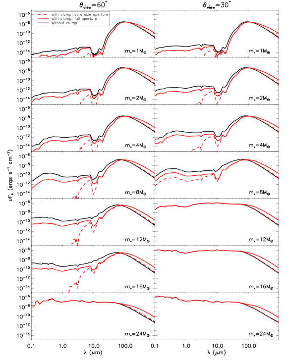
Figure 27.— SEDs for the seven evolutionary stages (from top to bottom: $m_{*}=1$, 2, 4, 8, 12, 16, and 24 $M_{\odot}$) at inclinations of $60^{\circ}$ (left) and $30^{\circ}$ (right) between the line of sight and the axis. In each panel, the fiducial model which does not contain the ambient clump (black curves) is compared to its variant with the clump (red curves). For those with the clump, we show both the SEDs observed with an aperture containing the whole clump (solid curves), and those observed with an aperture of the core size (dashed curves). A distance of 1 kpc is assumed.

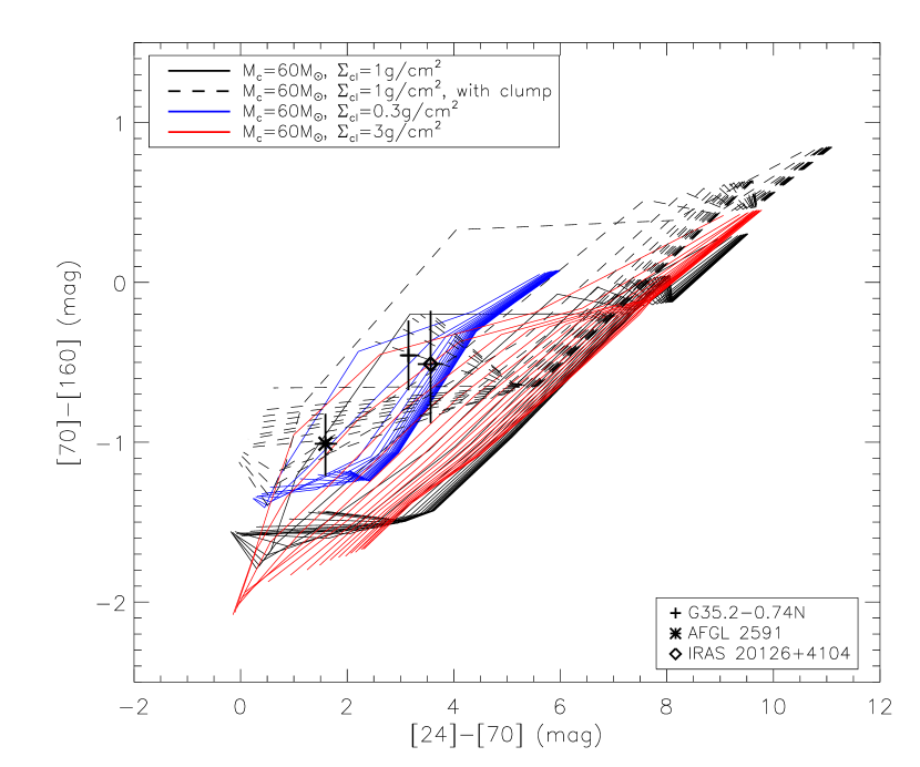
Figure 28.— Evolutionary tracks on the color-color diagram. The fiducial models, two of its variants with higher and lower $\Sigma_{\rm cl}$, and the fiducial model + the clump (with an intermediate aperture between the full aperture to cover the whole clump and the core-size aperture) are shown. For each model, the lines represent certain viewing angles, which are evenly distributed in the cosine space. Therefore a group of these lines shows the region a model will occupy at different evolutionary stages and inclinations. The three observational data points are G35.2-0.74N (Zhang et al. 2013b), AFGL 2591 (Johnston et al. 2013), IRAS 20126+4104 (Johnston et al. 2011). If the fluxes at the chosen wavelengths are not directly provided in these literatures, they are estimated by interpolating the SED. 20% uncertainties are added if not provided.

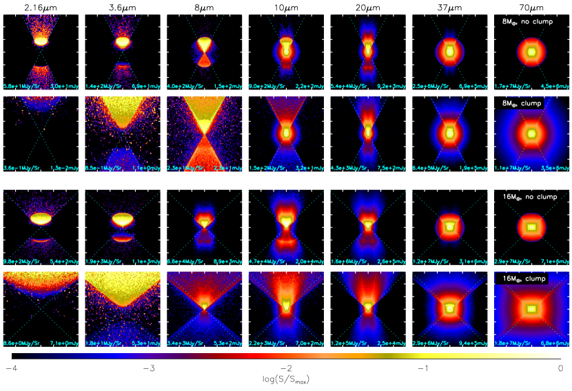
Figure 29.— Resolved images at various wavelengths (columns) at the evolutionary stages $m_{*}=8\>M_{\odot}$ (upper two panels) and $16\>M_{\odot}$ (lower two panels) at the inclination of $60^{\circ}$ between the line of sight and the axis. At each of the evolutionary stages, the fiducial model which does not include the ambient clump is compared to its variant with the clump included. Each image is normalized to its maximum surface brightness, which is labeled in the lower-left corner. The total fluxes are labeled in the lower-right corners. A distance of 1 kpc is assumed. Each image has a field of view of $60\arcsec\times 60\arcsec$. The dotted lines mark the projected opening angle of the outflow cavity on the sky plane.

As the Core Accretion model predicts, the protostellar core is embedded in a larger star-cluster-forming gas clump, and has pressure balance across the the core boundary. The properties of the core are affected by this clump environment. Although we use the mean mass surface density of the clump, $\Sigma_{\rm cl}$, to self-consistently set the conditions for the core and its evolution, the surrounding clump itself provides additional extinction and emission, which will affect the SEDs and images. Here we construct a variant of the fiducial model to include a clump with very simple structures, and briefly discuss how such a clump would affect the SED and images.

We assume the clump density decreases with the spherical radius as a power law $\rho_{\mathrm{cl}}\propto r^{-k_{\rho,\mathrm{cl}}}$, with the power-law index $k_{\rho,\mathrm{cl}}=1$ (Butler & Tan 2012). The clump starts at the core boundary with a density which is half of the core density at the boundary. Such a clump is extended to $\sim 8.8\>R_{c}$ so that the total surface density (including both the front and back sides of the core) reaches the assumed fiducial value $\Sigma_{\rm cl}=1\>{\rm g}\,{\rm cm}^{-2}$. The evolution of the core, the star, the disk and the outflow is all the same as in the fiducial model. SEDs with or without the clump are shown in Figure 27. For the model with the clump, we show SEDs observed with two different apertures. With an aperture of the core size, we exclude the emission from the clump outside the core on the sky plane, but not that in front of the core, i.e. the clump mainly acts as additional foreground extinction. Therefore the observed SEDs are much lower at wavelengths shorter than $\sim 100\>\mu$m than in the model with no clump. The SEDs are not affected if the line of sight towards the star passes through the outflow cavity. With a full aperture, we integrate over a region large enough to cover the whole model source including the clump on the sky plane. In such a case, the observed SEDs are significantly higher at the wavelengths longer than $\sim 100\>\mu$m. The short wavelength emission is lower than the model without the clump but higher than that observed with a smaller aperture at wavelengths $<10\>\mu$m. This is because the short wavelength emission can be seen towards the opening area of the outflow cavity, and this part of the emission is excluded with a smaller aperture. In real observations, depending on the resolutions in different bands, the observed SEDs may be similar to the model SED with smaller aperture in short wavelengths, but similar to the model SED with full aperture in long wavelengths, i.e., the short wavelength fluxes are strongly suppressed but the fluxes at $\gtrsim 100\>\mu$m becomes higher with the clump.

The influence of the clump on the SED can also be reflected on the color-color diagram. Figure 28 shows the evolutionary tracks of models with different $\Sigma_{\rm cl}$ without the clump. Three real sources are shown for reference: G35.2-0.74N (Zhang et al. 2013b), AFGL 2591 (Johnston et al. 2013), IRAS 20126+4104 (Johnston et al. 2011). The colors are calculated with fluxes either provided in the above literatures, or from interpolating the well sampled SEDs presented in these works. Although the locations of these three sources are covered by some of the models, especially the model with lower $\Sigma_{\rm cl}=0.3\>{\rm g}\,{\rm cm}^{-2}$, the sources appear significantly more red than the models. On such a diagram, the model with a clump also appears to be more red than the models without a clump. An intermediate aperture is chosen here to yield tracks that cover the locations of the real sources. If the offsets between the models and observations are due to the ambient clump, from the colors it seems that these three sources are all at later stages with $m_{*}\gtrsim 8\>M_{\odot}$, which agrees with the above literature estimates.

The effects of the clump on the images are shown in Figure 29. At wavelengths longer than $\sim 40\>\mu$m, the clump contributes to the extended emission. At wavelengths of 8, 10 and 20 $\mu$m, the emission is from the warm outflow cavity wall and hot inner region, with the clump, we see a more extended outflow cavity structure. At $\gtrsim 20\>\mu$m, the intensity distribution and the morphology of the bright part are not affected by the clump. At shorter wavelengths, which is dominated by the scattered light, the existence of the clump makes more emission come from the farther opening area of the outflow cavity, the innermost region becomes relatively dimmer.

4.2. Implications for Modeling Observed Sources

The models developed in Paper I and II were used to explain observations of a massive protostar G35.2-0.74N (Zhang et al. 2013b), by fitting both the SEDs and the intensity profiles along the outflow axis. Here we briefly discuss how the improved model we present here would affect the modeling of the observations.

First, unlike the model in Paper I and II, we now have a self-consistent model describing how the outflow cavity gradually opens up, therefore we can better model the observed lateral intensity distribution across the outflow cavity to constrain the opening angle of the outflow. From Figure 21, the observed morphologies of G35.2-0.74N at 10, 20 and 40 $\mu$m are similar to those at the stages $m_{*}$ = 8 or 12 $M_{\odot}$, i.e., an outflow cavity with an opening angle of $\sim 30^{\circ}$ (from axis to the cavity wall) with an inclination of $\sim 60^{\circ}$ can produce a similar IR morphology to this source. For a more massive core, an outflow cavity evolves to this size at higher stellar masses, e.g., $m_{*}\sim 32\>M_{\odot}$ in a core with initial 240 $M_{\odot}$ mass. Such a stellar mass agrees with our estimate from the bolometric luminosity.

Second, as discussed in the previous section, the core is embedded in a larger clump. Our model with a simplified clump structure suggests that the clump can significantly affect the SED and images. In reality, the clump (and indeed the core) can be highly turbulent and thus much more complicated than that in our model. Therefore, appropriately subtracting the contribution of the clump from the SED and the image is important in modeling the observations. A recent high resolution sub-mm interferometric observation (Qiu et al. 2013) reveals multiple cores within a scale of $10\arcsec$ near to the center of this source (22000 AU at a distance of 2.2 kpc), with one of the cores associated with the observed IR outflow cavity. The other cores in the turbulent clump contribute to the long wavelength emission, and are not resolved in the far-IR observations. A more accurate fitting with the model can be done with the contribution from these cores carefully estimated and subtracted.

5. Summary

We have constructed radiation transfer models for individual massive star formation, covering the whole evolutionary sequence, for various initial conditions of massive star formation.

1. Based on the model constructed for a single evolutionary stage presented in Papers I and Paper II, we now self-consistently calculate the evolution of the opening angle of the outflow, the instantaneous star-formation efficiency, the accretion rate, the size of the disk and the protostellar properties. The initial conditions are assumed based on the Turbulent Core model (MT03), and the collapse is described with an inside-out expansion wave solution (Shu 1977; McLaughlin & Pudritz 1997). The evolution of the outflow opening angle is determined by the criteria that the momentum of a disk wind is strong enough to sweep up the core (Matzner & McKee 2000). The protostellar evolution is improved with a detailed multi-zone model (Hosokawa & Omukai 2009; Hosokawa et al. 2010). In such a framework, an evolutionary track is determined by three environmental initial conditions: the initial core mass $M_{c}$, the mean surface density of the ambient clump $\Sigma_{\rm cl}$, and the rotational to gravitational energy ratio in the initial core $\beta_{c}$. In the fiducial model with $M_{c}=60\>M_{\odot}$, $\Sigma_{\rm cl}=1\>{\rm g}\,{\rm cm}^{-2}$ and $\beta_{c}=0.02$, the final mass of the protostar can reach $\sim 26\>M_{\odot}$, making the final average star formation efficiency $\gtrsim 0.43$. Other models with different initial conditions also have similar efficiencies, with a trend that a higher efficiency is achieved at higher $\Sigma_{\rm cl}$.

2. The projected temperature maps at different evolutionary stages are shown, which potentially can be compared with observations. As the protostar grows, the mass-weighted temperature of the envelope can increase by $\sim$ 30 K. The temperature of the core in a high surface density environment is much warmer than that in a low surface density region, because the core in a high $\Sigma_{\rm cl}$ environment is denser and more compact, leading to a higher accretion rate and luminosity. The temperature of the envelope is not so dependent on the initial core mass, although with a more massive and thus larger core, in the early stages the mean temperature is slightly lower because of the cold material in the outer region. In later stages, the envelope temperature is affected by the development of the outflow cavity.

3. SEDs of the models with different star formation efficiency, protostellar evolution, environmental mass surface densities and disk sizes are presented. To correctly explain an observation, a realistic evolutionary model of the star-formation efficiency and the outflow opening angle is required, while the effects of different protostellar evolution models are smaller. Generally, as the protostar grows, the fluxes at wavelengths shorter than $\sim 100\mu$m increase dramatically while the fluxes at longer wavelengths do not change much; the far-IR peaks also move to shorter wavelengths. The SEDs are affected by the environmental surface density $\Sigma_{\rm cl}$ due to the different accretion rates, extinctions, and evolutions of the outflow cavities and the protostars. We explored the effects of different disk sizes on the SED by adjusting the value of $\beta_{c}$. A change of a factor of 25 in the disk size has a relatively small impact on the SED at wavelengths $\gtrsim 20\>\mu$m, especially when the line of sight passes through the envelope so that the disk is less exposed. Derived from SEDs, the bolometric temperature increases rapidly from $<100$ K to $>1000$ K as the outflow cavity opens up, which may be used as an indicator of evolutionary stages. However, it is strongly affected by the inclination and the potential contribution of the cold ambient material.

4. We studied how the inferred luminosity depends on the viewing angle (the flashlight effect) and its evolution with the growth of the protostar. Compared to the true bolometric luminosity, the inferred luminosity from SED can be higher or lower by a factor of several depending on whether the source is face-on or edge-on, once a wide-angle outflow cavity has developed. Such a factor needs to be considered when using the SED to infer the luminosity and estimate the mass of the protostar.

5. We find the color-color diagram at long wavelengths (such as the color [$24\mu$m]-[$70\mu$m], [$70\mu$m]-[$160\mu$m]) can be a useful tool to determine the evolutionary stages of a massive protostar. The scatter caused by the inclination can be minimized using colors at these long wavelengths. Additional scatter is caused by initial conditions like the core mass and the surface density of the environment, but a general trend of evolutionary sequences can be clearly seen on such a color-color diagram. And we find that at early and late stages, the color is more dependent on $m_{*}/M_{c}$, while in the middle stages, the color is affected by the swelling phase of the protostar, and more dependent on the relative stage of protostellar evolution. The fast color change due to the swelling phase of protostellar evolution may cause massive protostars appear as two groups on such a color-color diagram.

6. Images of the fiducial model at selected evolutionary stages and observational bands are presented. The development of the outflow cavity with a gradually wider opening angle is seen on the images especially at $\sim 10-20\mu$m. Intensity profiles along and perpendicular to the outflow axis are shown. Such profiles can be compared to the observations to constrain the properties of the outflows from massive protostars, such as the opening angle and the inclination. The near-facing and far-facing sides of the outflow become more symmetric as the source is observed at a longer wavelength, or if the source is in an environment of a lower surface density. The profiles are affected by the evolution of the source due to several reasons, including the gradually lower extinction of the envelope, wider outflow cavity, and warmer outer envelope as the protostar grows.

7. We compared the SEDs, color-color diagram, and images of models with or without the ambient star-cluster-forming clump surrounding the protostellar core. Such a clump provides additional extinction at short wavelengths and emission at long wavelengths, both of which can significantly affect the observed SED and the position on the color-color diagram. Including the clump also produces a more extended envelope and outflow cavity structure. Although our model of the clump is very simple, its impact on the SEDs and images suggest that it is important to carefully estimate the contribution from the ambient clump material when comparing the model to the observations.

References

- Andre et al. (2000) Andre, P., Ward-Thompson, D., Barsony, M., 2000, in Protostars and Planets IV, ed. V. Mannings (Tucson: University of Arizona Press), 59
- Blandford & Payne (1982) Blandford, R. D., Payne, D., G., 1982, MNRAS, 199, 883
- Bonnell et al. (2001) Bonnell, I. A., Bate, M. R., Clarke, C. J., Pringle, J. E., 2001, MNRAS, 323, 785
- Bonnell et al. (1998) Bonnell, I. A., Bate, M. R., Zinnecker, H., 1998, MNRAS, 298, 93
- Brogan et al. (2011) Brogan, C. L., Hunter, T. R., Cyganowski, C. J., Friesen, R. K., Chandler, C. J., Indebetouw, R., 2011, ApJ, 739, L16
- Butler & Tan (2012) Butler, M. J., Tan, J. C., 2012, ApJ, 754, 5
- Butler et al. (2014) Butler, M. J., Tan, J. C., Kainulainen, J., 2014, ApJ, 782, L30
- Chen et al. (2012) Chen, X., Arce, H. G., Dunhan, M. M., Zhang, Q., 2012, ApJ, L43
- Dunham et al. (2014) Dunham, M. M., Stutz, A., Allen, L. E., et al., 2014, in Protostars and Planets VI, ed. H. Beuther, R. S. Klessen, C. P. Dulle- mond, & T. Henning (University of Arizona Press), in press, arXiv:1401.1809
- Fontani et al. (2011) Fontani, F., Palau, A., Caselli, et al., 2011, A&A, 529, L7
- Goodman et al. (1993) Goodman, A. A., Benson, P. J., Fuller, G. A., Myers, P. C., 1993, ApJ, 406, 528
- Hosokawa et al. (2011) Hosokawa, T., Offner, S. S. R., Krumholz, M. R., 2011, ApJ, 738, 140
- Hosokawa & Omukai (2009) Hosokawa, T., Omukai, K., 2009, ApJ, 691, 823
- Hosokawa et al. (2010) Hosokawa, T., Yorke, H. W., Omukai, K., 2010, ApJ, 721, 478
- Johnston et al. (2011) Johnston, K. G., Keto, E., Robitaille, T. P., Wood, K., 2011, MNRAS, 415, 2953
- Johnston et al. (2013) Johnston, K. G., Shepherd, D. S., Robitaille, T. P., Wood, K., A &A, 551, A43
- Königl & Pudritz (2000) Königl, A., Pudritz, R. E., 2000, in Protostars and Planets IV, ed. V. Mannings (Tucson: University of Arizona Press), 759
- Kratter et al. (2008) Kratter, K. M., Matzner, C. D., Krumholz, M. R., 2008, ApJ, 681, 375
- Li et al. (2012) Li, J., Wang, J., Gu, Q., Zhang, Z.-Y., Zheng, X., 2012, ApJ, 745, 47
- Li et al. (2013) Li, Z.-Y., Krasnopolsky, R., Shang, H., 2013, ApJ, 774, 82
- Matzner & McKee (1999) Matzner, C. D., McKee, C. F., 1999, ApJ, 526, L109
- Matzner & McKee (2000) Matzner, C. D., McKee, C. F., 2000, ApJ, 545, 364
- McKee & Tan (2002) McKee, C. F., Tan, J. C., 2002, Nature, 416, 59
- McKee & Tan (2003) McKee, C. F., Tan, J. C., 2003, ApJ, 585, 850
- McLaughlin & Pudritz (1997) McLaughlin, D. E., Pudritz, R. E., 1997, ApJ, 476, 750
- Molinari et al. (2008) Molinari, S., Pezzuto, S., Cesaroni, R., Brand, J., Faustini, F., Testi, L., 2008, A&A, 481, 345
- Myers & Ladd (1993) Myers, P. C., Ladd, E. F., 1993, ApJ, 413, L47
- Nakano et al. (2000) Nakano, T., Hasegawa, T., Morino, J.-I., Yamashita, T., 2000, ApJ, 534, 976
- Nakano et al. (1995) Nakano, T., Hasegawa, T., Norman, C., 1995, ApJ, 450, 183
- Ostriker (1997) Ostriker, E. C., 1997, ApJ, 486, 291
- Palau et al. (2013) Palau, A., Fuente, A., Girart, J. M., et al., 2013, ApJ, 762, 120
- Palla & Stahler (1991) Palla, F., Stahler, S. W. 1991, ApJ, 375, 288
- Qiu et al. (2013) Qiu, K., Zhang, Q., Menten, K. M., Liu, H. B., Tang, Y.-W., 2013, arxiv:astro-ph/1311.0566
- Robitaille et al. (2006) Robitaille, T. P., Whitney, B. A., Indebetouw, R., Wood, K., Denzmore, P., 2006, ApJS, 167, 256
- Schaller et al. (1992) Schaller, G., Schaerer, D., Meynet, G., Maeder, A, 1992, A&AS, 96, 269
- Shakura & Sunyaev (1973) Shakura, N. I., Sunyaev, R. A., 1973, A&A, 24, 337
- Shu (1977) Shu, F. H., 1977, ApJ, 214, 488
- Shu et al. (1995) Shu, F. H., Najita, J. R., Ostriker, E. C., Shang, H., 1995, ApJ, 455, L155
- Stahler et al. (1980) Stahler, S. W., Shu, F. H., Taam, R. E., 1980, ApJ, 241, 637
- Stahler et al. (1986) Stahler, S. W., Palla, F., Salpeter, E. E., 1986, ApJ, 302, 590
- Tan et al. (2014) Tan, J. C., Beltrán, M. T., Caselli, P., et al., 2014, in Protostars and Planets VI, ed. H. Beuther, R. S. Klessen, C. P. Dullemond, & T. Henning (University of Arizona Press), in press, arXiv:1402.0919
- Tan & McKee (2002) Tan, J. C., McKee, C. F., 2002, in ASP Conf. Ser. 267, Hot Star Workshop III: The Earlist Phases of Massive Star Birth, ed. P. Crowther, p267
- Tan & McKee (2004) Tan, J. C., McKee, C. F., 2004, ApJ, 603, 383
- Ulrich (1976) Ulrich, R. K., ApJ, 210, 377
- Wang et al. (2010) Wang, P., Li, Z., Abel, T., Nakamura, F., 2010, ApJ, 709, 27
- Whitney et al. (2013) Whitney, B. A., Robitaille, T. P., Bjorkman, J. E., Dong, R., Wolff, M. J., Wood, K., Honor, J., 2013, ApJS, 207, 30
- Whitney et al. (2003) Whitney, B. A., Wood, K., Bjorkman, J. E., Wolff, M. J., 2003, ApJ, 591, 1049
- Yorke & Bodenheimer (1999) Yorke, H. W., Bodenheimer, P., 1999, ApJ, 525, 330
- Zhang & Tan (2011) Zhang, Y., Tan, J. C., 2011, ApJ, 733, 55
- Zhang et al. (2013b) Zhang, Y., Tan, J. C., De Buizer, J. M., Beltran, M. T., Churchwell, E.,
- Zhang et al. (2013a) Zhang, Y., Tan, J. C., McKee, C. F., 2013, ApJ, 766, 86 McKee, C. F., Sandell, G., Shuping, R., Staff, J. E., Telesco, Whitney, B., 2013, ApJ, 767, 58