Neutron matter under strong magnetic fields: a comparison of models

Abstract

The equation of state of neutron matter is affected by the presence of a magnetic field due to the intrinsic magnetic moment of the neutron. Here we study the equilibrium configuration of this system for a wide range of densities, temperatures and magnetic fields. Special attention is paid to the behavior of the isothermal compressibility and the magnetic susceptibility. Our calculation is performed using both microscopic and phenomenological approaches of the neutron matter equation of state, namely the Brueckner–Hartree–Fock (BHF) approach using the Argonne V18 nucleon-nucleon potential supplemented with the Urbana IX three-nucleon force, the effective Skyrme model in a Hartree–Fock description, and the Quantum Hadrodynamic formulation with a mean field approximation. All these approaches predict a change from completely spin polarized to partially polarized matter that leads to a continuous equation of state. The compressibility and the magnetic susceptibility show characteristic behaviors, which reflect that fact. Thermal effects tend to smear out the sharpness found for these quantities at T=0. In most cases a thermal increase of $\Delta T=10$ MeV is enough to hide the signals of the change of polarization. The set of densities and magnetic field intensities for which the system changes it spin polarization is different for each model. However, we found that under the conditions examined in this work there is an overall agreement between the three theoretical descriptions.

I Introduction

The effects of magnetic fields on dense matter have been a subject of interest for a long time (see e.g., Ref. LAI and references therein), particularly in relation to astrophysical issues. The equation of state for magnetized matter is important for the neutron star structure LATTIMER and for the cooling of magnetized stars SHIBANOV ; YAKOVLEV ; BEZCHASTNOV . Moreover, since neutrinos have a fundamental role in cooling processes, their emission and transport properties in the presence of magnetic fields have also been studied in detail YAKOVLEV ; BEZCHASTNOV . A wide range of observational data of periodic or irregular radiation from localized sources has been related to the presence of very intense magnetic fields in compact stellar objects. These manifestations have been associated with pulsars, soft gamma ray repeaters and anomalous X-ray pulsars, according to the energy released and the periodicity of the episodes. Thus, they have been associated with different stages of the evolution of neutron stars. The intensity of the magnetic fields could reach values, e.g., in the case of magnetars, up to $10^{14}-10^{15}$ G in the star surface and grows by several orders of magnitude in its dense interior. The origin of such unusually large intensities is still uncertain. A possible explanation invokes a spontaneous phase transition to a ferromagnetic state at densities corresponding to theoretically stable neutron stars and therefore a ferromagnetic core in the liquid interior of such compact objects. Such possibility has been considered since long ago by many authors within different theoretical approaches (see e.g., Refs. BROWNELL ; RICE ; CLARK ; CLARK2 ; SILVERSTEIN ; OST ; PEAR ; PANDA ; BACK ; HAENSEL ; JACK ; KUT ; MARCOS ; VIDAURRE ; RIOS ; GOGNY ; FANTONI ; VIDANA ; VIDANAb ; VIDANAc ; SAMMARRUCA1 ; SAMMARRUCA2 ; BIGDELI ), but results were contradictory. Whereas some calculations based on Skyrme VIDAURRE ; RIOS or Gogny GOGNY interactions predicted such a transition to occur at densities in the range $(1-4)n_{0}$ ($n_{0}=0.16$ fm^-3), other calculations that used modern two- and three-body realistic interactions, like Monte Carlo FANTONI , Brueckner–Hartree–Fock (BHF) VIDANA ; VIDANAb ; VIDANAc , Dirac–Brueckner–Hartree–Fock SAMMARRUCA1 ; SAMMARRUCA2 , or lowest-order constraint variational BIGDELI , excluded such a transition. Nowadays, there is a general consensus that the ferromagnetic instability predicted by the Skyrme forces at high densities is in fact a pathology of such forces. Modifications of the standard Skyrme interaction have been recently proposed SAGAWA ; CHAMEL in order to remove the instability.

Recently it was pointed out KHARZEEV ; MO ; SKOKOV that matter created in heavy ion collisions could be subject to very strong magnetic fields, with distinguishable consequences on particle production. In Ref. KHARZEEV a magnetic field is predicted in noncentral heavy ion collisions such that $e\,B\sim 10^{2}$ MeV², which would be the cause of a preferential emission of charged particles along the direction of the magnetic field. Improvements in the description of the mass distribution of the colliding ions MO does not modify essentially the magnitude of the fields produced. On the other hand, the numerical simulations performed by SKOKOV predicts values $e\,B\sim m_{\pi}^{2}$ MeV², which are much larger than those in Ref. KHARZEEV .

Several models have been used to describe the effects of magnetic fields in a dense nuclear environment and particularly on the properties and the structure of neutron stars CHAKRABARTY ; BRODERICK ; YUE2 ; SINHA ; RABHI2 ; RABHI0b ; RYU ; RYU2 ; RABHI3 ; ANG ; DONG ; DIENER ; DONG2 ; PGARCIA ; ISAEV2 ; UNLP ; BORDBAR ; BIGDELI2 . Among them, covariant field theoretical models have been extensively used to study the role of the magnetic field in hyperonic matter YUE2 ; SINHA , instabilities at subsaturation densities RABHI2 ; RABHI0b ; RYU , magnetization of stellar matter DONG , saturation properties of symmetric matter DIENER , and the symmetry energy DONG2 . Non-relativistic models have also been used in this context PGARCIA ; ISAEV2 ; UNLP and microscopic models based on realistic nucleon forces, such as the recent lowest-order variational calculations of Refs. BORDBAR and BIGDELI2 .

Due to its important applications, as well as to its intrinsic theoretical interest, a comparison of predictions is in order. Therefore, we have selected three models, of very different origins, to study the properties of infinite homogeneous neutron matter in the presence of strong magnetic fields. They are the Brueckner–Hartree–Fock (BHF) approach using the Argonne V18 nucleon-nucleon potential supplemented with the Urbana IX three-nucleon force, the covariant formulation known as Quantum Hadro-dynamics (QHD), and the non-relativistic Skyrme effective potential. It would be interesting to include a comparison with other microscopic calculations, as for instance with the auxiliary field diffusion Monte Carlo (AFDMC) method FANTONI ; AFDMC . As an interesting precedent, it must be mentioned that a comparison between the BHF and AFDMC approaches was already done in Ref. VIDANA . The results for the magnetic susceptibility of spin polarized neutron matter at zero temperature in the absence of a magnetic field, give a remarkable agreement between the two methods.

In the present work, we focus on the polarization of neutron matter by analyzing its dependence with density, magnetic field and temperature. In order to understand this behavior, we also consider the energy of the system and its pressure. In addition, we pay special attention to some thermodynamical coefficients: the isothermal compressibility and the magnetic susceptibility. We consider a range of densities where nucleons are the main degrees of freedom of hadronic matter, and temperatures and field intensities up to $T=10$ MeV and $B=10^{19}$ G, respectively.

This article is organized as follows. A brief review of the properties of spin polarized neutron matter and of the models and approximations used is presented in the next section, and the results are shown and discussed in Section III. A final summary and the main conclusions are given in Section IV.

II Neutron matter in an external magnetic field

Spin polarized neutron matter is an infinite nuclear system made of two different fermionic components: neutrons with spin up and neutrons with spin down, having number densities $n_{\uparrow}$ and $n_{\downarrow}$, respectively. Hence, the total number density is given by

$$n=n_{\uparrow}+n_{\downarrow}\ .$$ (1)

The degree of spin polarization of the system can be expressed by means of the spin asymmetry density, defined as

$$W=n_{\uparrow}-n_{\downarrow}\ .$$ (2)

Note that the value $W=0$ corresponds to nonpolarized neutron matter, whereas $W=n$ or $W=-n$ means, respectively, that the system is in a completely polarized state with all the spins up (CPS-U) or down (CPS-D), i.e., all the spins are aligned along the same direction. Partially polarized states (PPS) correspond to values of $W$ between $-n$ and $n$.

In the following we present the main features of the three approaches used to describe the properties of spin-polarized neutron matter in the presence of an external magnetic field B. We evaluate first, for the three approaches, the Helmhotz free-energy density of the system ${\mathcal{F}}={\mathcal{E}}-T{\mathcal{S}}$, where the energy density ${\mathcal{E}}$ includes the term describing the interaction of matter with the external field, and the entropy density ${\mathcal{S}}$ is evaluated in the quasi-particle approximation. Then, we determine from ${\mathcal{F}}$ other macroscopic properties of the system such as the pressure $P$, the magnetization of the system per unit volume

$${\cal M}=\left(\frac{\partial P}{\partial B}\right)_{\mu,T,\Omega}\ ,$$ (3)

the isothermal compressibility

$$K=-\frac{1}{\Omega}\left(\frac{\partial\Omega}{\partial P}\right)_{N,T,B}$$ (4)

where $\Omega$ is the volume of the system, and the magnetic susceptibility

$$\chi=\left(\frac{\partial{\cal M}}{\partial B}\right)_{N,T,\Omega}$$ (5)

which characterizes the response of the system to the external field and gives a measure of the energy required to produce a net spin alignment in the direction of the field.

From here on we use units such that $\hbar=1$, $c=1$, and $k_{B}=1$.

II.1 The BHF approach

The extension of the BHF approach for neutron matter in the presence of a magnetic field and finite temperature starts with the construction of the neutron-neutron $G$-matrix. It describes, in an effective way, the interaction between two neutrons for any spin combination. This is formally obtained by solving the well known Bethe–Goldstone equation

$$\langle{\vec{k}_{3}}\sigma_{3},{\vec{k}_{4}}\sigma_{4}|G(\omega)|{\vec{k}_{1}}\sigma_{1},{\vec{k}_{2}}\sigma_{2}\rangle=\langle{\vec{k}_{3}}\sigma_{3},{\vec{k}_{4}}\sigma_{4}|V|{\vec{k}_{1}}\sigma_{1},{\vec{k}_{2}}\sigma_{2}\rangle$$

$$+\frac{1}{\Omega}\sum_{\sigma_{i}{\vec{k}_{i}},\sigma_{j}{\vec{k}_{j}}}\langle{\vec{k}_{3}}\sigma_{3},{\vec{k}_{4}}\sigma_{4}|V|{\vec{k}_{i}}\sigma_{i},{\vec{k}_{j}}\sigma_{j}\rangle\frac{Q_{\sigma_{i}\sigma_{j}}({\vec{k}_{i}},{\vec{k}_{j}})}{\omega-\epsilon_{\sigma_{i}}-\epsilon_{\sigma_{j}}+i\eta}\langle{\vec{k}_{i}}\sigma_{i},{\vec{k}_{j}}\sigma_{j}|G(\omega)|{\vec{k}_{1}}\sigma_{1},{\vec{k}_{2}}\sigma_{2}\rangle$$ (6)

where $\sigma=\uparrow,\downarrow$ indicates the spin projection of each neutron in the initial, intermediate and final states, $V$ is the bare nucleon-nucleon interaction, $Q_{\sigma_{i}\sigma_{j}}({\vec{k}_{i}},{\vec{k}_{j}})=(1-\nu_{\sigma_{i}}({\vec{k}_{i}}))(1-\nu_{\sigma_{j}}({\vec{k}_{j}}))$, where $\nu_{\sigma}({\vec{k}})$ is the occupation number defined in Eq. (9), is the Pauli operator which allows only intermediate states compatible with the Pauli principle, and $\omega$ is the so-called starting energy defined as the sum of the non-relativistic single-particles energies $\epsilon_{\uparrow(\downarrow)}$ of the interacting neutrons. Note that Eq. (6) is a coupled channel equation.

The single-particle energy of a neutron with momentum ${\vec{k}}$ and spin projection $\sigma$ in the presence of an external magnetic field $B$ is given by

$$\epsilon_{\sigma}({\vec{k}})=\frac{k^{2}}{2m}+\mbox{Re}[U_{\sigma}({\vec{k}})]\mp\kappa B\ ,$$ (7)

where the real part of the single-particle potential $U_{\sigma}({\vec{k}})$ represents the average potential “felt” by a neutron in the nuclear medium. The minus (plus) sign in the last term corresponds to neutrons with spin up (down), and $\kappa=-1.913\mu_{N}$ is the anomalous magnetic moment of the neutron with $\mu_{N}$ the nuclear magneton. In the BHF approximation $U_{\sigma}({\vec{k}})$ is given by

$$U_{\sigma}({\vec{k}})=\frac{1}{\Omega}\sum_{\sigma^{\prime},{\vec{k}^{\prime}}}\nu_{\sigma^{\prime}}({\vec{k}^{\prime}})\langle{\vec{k}}\sigma,{\vec{k}^{\prime}}\sigma^{\prime}|G(\omega=\epsilon_{\sigma}(\vec{k})+\epsilon_{\sigma^{\prime}}(\vec{k}^{\prime}))|{\vec{k}}\sigma,{\vec{k}^{\prime}}\sigma^{\prime}\rangle_{A}$$ (8)

where the occupation number of a neutron with spin projection $\sigma$ at zero temperature is

$$\nu_{\sigma}({\vec{k}})=\left\{\begin{array}[]{cc}1,&\mbox{if}\,\,|{\vec{k}}|\leq k_{F_{\sigma}}\\ 0,&\mbox{otherwise}\end{array}\right.$$ (9)

with $k_{F_{\sigma}}=(6\pi^{2}n_{\sigma})^{1/3}$ the corresponding Fermi momentum, and the matrix elements are properly antisymmetrized. We note here that the so-called continuous prescription JEKEUNE has been adopted for the single-particle potential when solving the Bethe–Goldstone equation. It has been shown by Song et al., SONG that the contribution to the energy from three-hole-line diagrams (which account for the effect of three-body correlations) is minimized when this prescription is adopted. This presumably enhances the convergence of the hole-line expansion of which the BHF approximation represents the lowest order. We also note that the present BHF calculation has been carried out using the Argonne V18 potential WIRINGA supplemented with the Urbana IX three-nucleon force PUDLINER , which for the use in the BHF approach is reduced first to an effective two-nucleon density-dependent force by averaging over the coordinates of the third nucleon TBF .

The total energy per unit volume is easily obtained once a self-consistent solution of Eqs. (6)-(8) is achieved

$${\mathcal{E}}=\frac{1}{\Omega}\sum_{\sigma{\vec{k}}}\nu_{\sigma}({\vec{k}})\left(\frac{k^{2}}{2m}+\frac{1}{2}\mbox{Re}[U_{\sigma}(\vec{k})]\right)-\kappa WB\ ,$$ (10)

where $W$ is the spin asymmetry density defined in Eq. (2).

For further purposes, it is convenient to introduce the effective mass $m_{\sigma}^{*}(k)$ defined as,

$$\frac{m_{\sigma}^{*}(k)}{m}=\frac{k}{m}\left(\frac{d\epsilon_{\sigma}(k)}{dk}\right)^{-1}\ ,$$ (11)

where $m$ is the bare neutron mass.

At the BHF level, finite temperature effects can be introduced in a very good approximation just by replacing the zero temperature limit of the occupation number, Eq (9), by its full expression

$$f_{\sigma}({\vec{k}},T)=\frac{1}{1+\exp[(\epsilon_{\sigma}({\vec{k}},T)-\mu_{\sigma}(T))/T]}\ ,$$ (12)

into the formulae shown in Eqs. (6), (8), and (10). Here $\mu_{\sigma}(T)$ is the chemical potential of a neutron with spin projection $\sigma$.

These approximations, valid in the range of densities and temperatures considered here, correspond to the “naive” finite temperature Brueckner–Bethe–Goldstone expansion discussed by Baldo and Ferreira in Ref. BF . The interested reader is referred to this work and references therein for a formal and general discussion on the nuclear many-body problem at finite temperature.

In this case, however, the self-consistent procedure implies that, together with the Bethe-Goldstone equation and the single-particle potential, the chemical potentials of neutrons with spin up and down must be extracted at each step of the iterative process from the normalization condition

$$n_{\sigma}=\frac{1}{\Omega}\sum_{\vec{k}}f_{\sigma}({\vec{k}},T)\ .$$ (13)

This is an implicit equation which can be solved numerically. Note that the $G$-matrix obtained from the Bethe–Goldstone equation (6) and also the single-particle potentials depend implicitly on the chemical potentials.

Once a self-consistent solution is achieved, the entropy per unit volume is calculated in the quasi-particle approximation

$${\mathcal{S}}=-\frac{1}{\Omega}\sum_{\sigma{\vec{k}}}\left(f_{\sigma}({\vec{k}},T)\mbox{ln}(f_{\sigma}({\vec{k}},T))+(1-f_{\sigma}({\vec{k}},T))\mbox{ln}(1-f_{\sigma}({\vec{k}},T))\right)\ ,$$ (14)

which together with the energy density ${\mathcal{E}}$ are used to evaluate the Helmhotz free energy density ${\mathcal{F}}$.

Finally, for fixed values of the total density $n$, the temperature $T$ and the external field $B$, the physical state is simply obtained by minimizing ${\mathcal{F}}$ with respect to the spin asymmetry density $W$. We note that this minimization implies that in the physical state $\mu_{\uparrow}=\mu_{\downarrow}$, i.e., there is only one chemical potential which is associated to the conservation of the total baryonic number.

II.2 The QHD model

QHD is a covariant formulation of field theory, where the nuclear interaction is mediated by the exchange of the following mesons: the scalar isoscalar $\sigma$-meson, the vector isoscalar $\omega$-meson, and the vector isovector $\rho$-meson. We adopt here the FSU-Gold model FSUGOLD , where a meson self-interaction is added to the ordinary nucleon-meson vertices. The lagrangian density reads

$${\mathcal{L}} = \bar{\psi}\left(i\not\!\partial-m+g_{\sigma}\sigma-g_{\omega}\not\!\omega-\frac{g_{\rho}}{2}\mathbf{\tau}\cdot\not\!\mathbf{\rho}+\kappa\sigma_{\mu\nu}F^{\mu\nu}\right)\psi+\frac{1}{2}(\partial^{\mu}\sigma\partial_{\mu}\sigma-m_{\sigma}^{2}\sigma^{2})$$

$$-\frac{g_{2}}{3}\,\sigma^{3}-\frac{g_{3}}{4}\,\sigma^{4}-\frac{1}{4}W^{\mu\nu}W_{\mu\nu}+\frac{1}{2}m_{w}^{2}\omega^{2}+\frac{C}{4}\,\omega^{4}-\frac{1}{4}R^{\mu\nu}\cdot R_{\mu\nu}+\frac{1}{2}m_{r}^{2}\rho^{2}+D\rho^{2}\;\omega^{2}$$

where we have used $\omega^{2}=\omega^{\mu}\omega_{\mu},\;\rho^{2}=\mathbf{\rho}^{\mu}\cdot\mathbf{\rho}_{\mu},\;W_{\mu\nu}=\partial_{\mu}\omega_{\nu}-\partial_{\nu}\omega_{\mu},\;R_{\mu\nu}=\partial_{\mu}\rho_{\nu}-\partial_{\nu}\rho_{\mu}$, $\sigma_{\mu\nu}=i[\gamma_{\mu},\gamma_{\nu}]/2$, and $F^{\mu\nu}$ is the electromagnetic tensor. Furthermore $g_{\sigma},g_{\omega},g_{\rho},g_{2},g_{3},C$, and $D$ are the coupling constants. We note that in the above expression the index “$\sigma$” should not be confused with the spin projection of the neutron.

In the mean field approximation the meson fields $\sigma,\omega,\rho$ are replaced by their corresponding in-medium expectation values $\langle\sigma\rangle,\langle\omega\rangle$ and $\langle\rho\rangle$ which obey the following equations of motion

$$\left(i\not\!\partial-m+g_{\sigma}\langle\sigma\rangle-g_{\omega}\gamma_{0}\langle\omega\rangle+\frac{1}{2}g_{\rho}\gamma_{0}\langle\rho\rangle+\kappa\sigma_{\mu\nu}F^{\mu\nu}\right)\psi = 0,$$ (15)

$$m_{\sigma}^{2}\langle\sigma\rangle+g_{2}\langle\sigma\rangle^{2}+g_{3}\langle\sigma\rangle^{3} = g_{\sigma}n_{s},$$ (16)

$$m_{\omega}^{2}\langle\omega\rangle+C\langle\omega\rangle^{3}+2D\langle\rho\rangle^{2}\langle\omega\rangle = g_{\omega}n,$$ (17)

$$m_{\rho}^{2}\langle\rho\rangle+2D\langle\omega\rangle^{2}\langle\rho\rangle = -g_{\rho}n$$ (18)

where

$$n=\langle\bar{\psi}\gamma_{0}\psi\rangle=\frac{1}{\Omega}\sum_{\sigma\vec{k}}f_{\sigma}({\vec{k}},T)$$ (19)

is the total number density and

$$n_{s}=\langle\bar{\psi}\psi\rangle=\frac{1}{\Omega}\sum_{\sigma\vec{k}}\frac{m^{*}}{E_{\sigma}({\vec{k}})}f_{\sigma}({\vec{k}},T)$$ (20)

is the scalar density, $m^{*}=m-g_{\sigma}\langle\sigma\rangle$ is the neutron effective mass and

$$E_{\sigma}({\vec{k}})=\sqrt{k^{2}_{//}+\left(\sqrt{m^{*\,2}+k^{2}_{\bot}}\mp\kappa B\right)^{2}}$$ (21)

the relativistic energy. Here one must distinguish the momentum components parallel ($k_{//}$) and perpendicular ($k_{\bot}$) to the magnetic field. As in Eq. (7) the minus (plus) sign in the above expression is for neutrons with spin up (down). The single-particle energy is given in this model by

$$\epsilon_{\sigma}({\vec{k}})=E_{\sigma}({\vec{k}})+g_{\omega}\langle\omega\rangle-\frac{1}{2}g_{\rho}\langle\rho\rangle\ ,$$ (22)

which corresponds to one of the eigenvalues of Eq. (15).

The energy per unit volume can be evaluated as the component $T^{00}$ of the energy-momentum tensor

$${\mathcal{E}} = \frac{1}{\Omega}\sum_{\sigma\vec{k}}f_{\sigma}({\vec{k}},T)E_{\sigma}({\vec{k}})+\frac{1}{2}\left((m_{\sigma}\langle\sigma\rangle)^{2}+(m_{\omega}\langle\omega\rangle)^{2}+(m_{\rho}\langle\rho\rangle)^{2}\right)$$ (23)

$$+ \frac{1}{3}g_{2}\langle\sigma\rangle^{3}+\frac{1}{4}g_{3}\langle\sigma\rangle^{4}+\frac{3}{4}C\langle\omega\rangle^{4}+3D(\langle\omega\rangle\langle\rho\rangle)^{2}$$

The magnetization has a simple expression

$${\cal M}=\frac{\kappa}{\Omega}\sum_{\sigma\vec{k}}sf_{\sigma}({\vec{k}},T)\frac{\sqrt{m^{*2}+\hbar^{2}k_{\bot}^{2}}-s\kappa B}{E_{\sigma}({\vec{k}})}$$ (24)

where $s=1(-1)$ for $\sigma=\uparrow(\downarrow)$.

II.3 The Skyrme model

The Skyrme model is an effective formulation of the nuclear interaction SKYRME . It consists of a two-body contact potential plus some terms having an explicit density dependence which, in an effective way, represent the effect of the three- and multi-body forces. Using this interaction in the Hartree–Fock approximation, one builds up an energy density functional. The associated single–particle spectrum can be expressed in such a way that the interaction contributes partly to the definition of an effective mass and partly to a remaining potential energy. In the present work we adopt the SLy4 parametrization from Ref. DOUCHIN .

In the presence of an external magnetic field $B$, the energy density functional is the sum of the standard Skyrme density functional plus the interacting term between matter and $B$,

$${\mathcal{E}}=\sum_{\sigma}\,\frac{K_{\sigma}}{2m^{*}_{\sigma}}+\frac{1}{16}\,a\,(n^{2}-W^{2})-\kappa WB,$$ (25)

where

$$K_{\sigma}=\frac{1}{\Omega}\sum_{\vec{k}}k^{2}f_{\sigma}({\vec{k}},T)$$ (26)

is the kinetic density, and we have introduced the effective nucleon mass $m^{*}_{\sigma}$ for a definite spin polarization state, defined as

$$\frac{1}{m^{*}_{\sigma}}=\frac{1}{m}+\frac{1}{4}\,(b_{0}\,n+s\,b_{1}\,W)$$ (27)

with as before $s=1(-1)$for $\sigma=\uparrow(\downarrow)$.

The single-particle spectrum is,

$$\epsilon_{\sigma}({\vec{k}})=\frac{k^{2}}{2m^{*}_{\sigma}}+\frac{1}{8}\,v_{\sigma}\mp\kappa B$$ (28)

which is obtained in a self–consistent way through the functional derivative $\epsilon_{\sigma}({\vec{k}})=\delta{\mathcal{E}}/\delta f_{\sigma}({\vec{k}},T)$. In Eq. (28) we have used,

$$v_{\sigma}=a\,(n\mp W)+\sum_{\sigma^{\prime}}(b_{0}+(2\delta_{\sigma\sigma^{\prime}}-1)b_{1})K_{\sigma^{\prime}}+\frac{\alpha}{3}t_{3}(1-x_{3})(n^{2}-W^{2})n^{\alpha-1},$$ (29)

where the last term corresponds to the rearrangement contribution.

The parameters $a,\,b_{0}$ and $b_{1}$ can be written in terms of the standard parameters of the Skyrme model,

$$a = 4t_{0}(1-x_{0})+\frac{2}{3}t_{3}(1-x_{3})n^{\alpha}$$

$$b_{0} = t_{1}(1-x_{1})+3t_{2}(1+x_{2})$$

$$b_{1} = t_{2}(1+x_{2})-t_{1}(1-x_{1}).$$

we have adopted $M=\kappa W$ for the magnetic moment of the system. For given values of $n$, $T$ and $B$ we solve in a self-consistent way the set of Eqs. (25)-(29), obtaining the spin polarization $W$ and the chemical potential $\mu$ that reproduces the density. The physical state corresponds to that configuration (among CPS-U, CPS-D and PPS) which gives the lowest value of ${\mathcal{F}}$.

We want to point out that here the physical state corresponds to a minimum of ${\cal F}$, in contrast with previous investigations of two of the authors UNLP , where a transformed thermodynamical potential was used.

III Results and discussion

Before we present our results we would like to make a comment on the validity and limitations of the models considered. Generally speaking, the validity of most of the nuclear models is questionable in the limit of high densities and high isospin asymmetries where the description of nuclear matter requires the inclusion of additional degrees of freedom and phenomena such as e.g., hyperons, meson condensates or the chiral and quark-gluon plasma phase transitions. In addition, the reader should also note that in the case of non-relativistic models, as e.g., BHF and Skyrme, causality is not always guaranteed at high densities. To avoid such problems and to highlight the aim of this work, we have restricted our calculations to densities below $2.5\,n_{0}$. The density and temperature domain chosen ensures an a priori reasonable agreement among the different theoretical descriptions. Taking into account the smallness of the neutron magnetic moment, we also expect that even the largest magnetic field considered in this work, $B=10^{19}$ G, will not modify essentially the dynamical regime of the nuclear interactions. We finish this comment by mentioning that, although, the SLy4 parametrization considered here shows an anomalous spontaneous magnetization at $n\simeq 4\,n_{0}$ ISAEV2 we do not expect it to have any influence in the subsaturation density region. Possible effects on the medium range densities will be timely commented.

In the following we discuss the results obtained for homogeneous neutron matter under a strong magnetic field, with the models and approximations described in the previous section. In all the figures, we show results corresponding to the physical state, i.e., that within the possible configurations CPS-U, CPS-D and PPS which gives a minimum value of the free-energy density ${\mathcal{F}}$. As the density, temperature, and field intensity changes, the system can pass from one global configuration to another. For example, for fixed temperature and intensity $B$ the system can pass from CPS-D to PPS as the density increases. In a similar way, for fixed density and temperature, an increase of the magnetic intensity leads the system from a PPS to a PPS-D. We define as threshold density $n_{t}$ (threshold field $B_{t}$) the value of the density (field) where the minimum free energy ${\mathcal{F}}$ changes from one state of polarization to another for fixed values of $B$ and $T$ ($n$ and $T$).

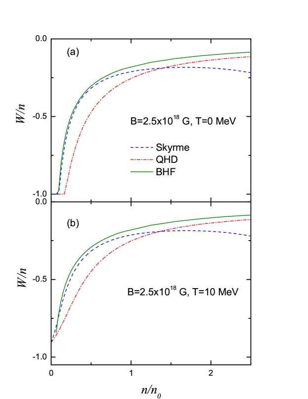
Figure 1: (Color online) Spin asymmetry as a function of the density at $B=2.5\times 10^{18}$ G and $T=0$ (panel a) and $T=10$ MeV (panel b) for the three models considered.

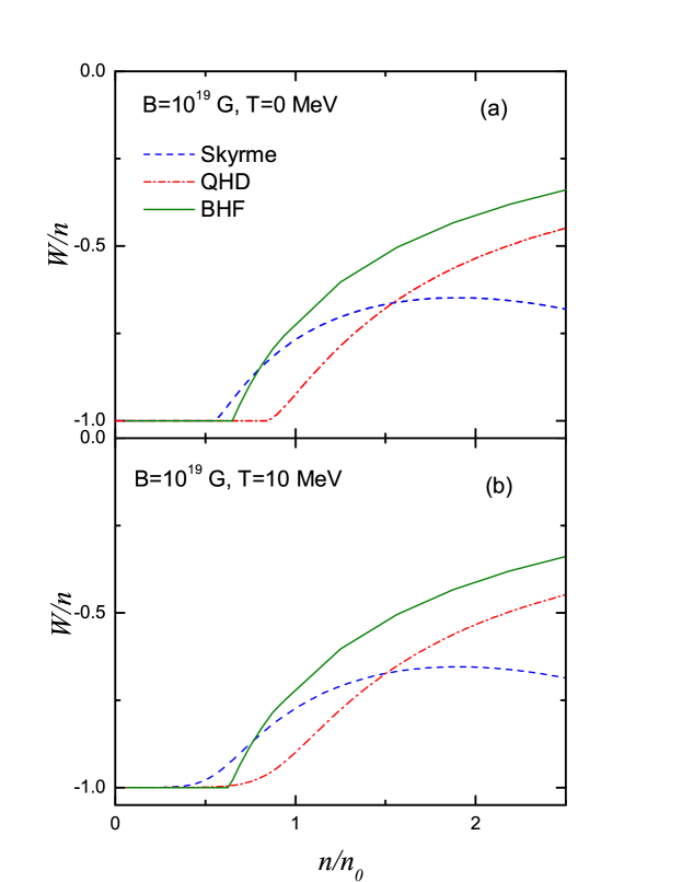
Figure 2: (Color online) Same as Fig. 1 for $B=10^{19}$ G.

We consider firstly the spin asymmetry density $W$, which gives us information about the global state of polarization of the system. In particular, Figs. 1 and 2 show the ratio $W/n$ in terms of the total neutron density, different magnetic field intensities and temperatures. At zero temperature (see Figs. 1(a) and 2(a)) and for very low densities, the system is completely polarized ($W/n=-1$) up to a threshold density, $n_{t}$, where it changes to partially polarized, with predominance of spin down states ($-1<W/n<0$). A comparison of the $B=2.5\times 10^{18}$ G (Fig. 1) and $B=10^{19}$ G (Fig. 2) cases, shows that the threshold density increases with $B$. However its precise location depends on the model used. For instance for $B=10^{19}$ G at $T=0$ (see Fig. 2a), we obtain $n_{t}/n_{0}=0.55$ for Skyrme, $n_{t}/n_{0}=0.65$ for BHF, and $n_{t}/n_{0}=0.85$ for QHD. It must be noted that beyond the threshold, both BHF and QHD predicts always a monotonous growth, reaching asymptotically the nonpolarized state ($W/n=0$) at high densities. On the contrary, for the Skyrme model, the system is always in a partially polarized state. This behavior is a consequence of the well known ferromagnetic instability predicted by the Skyrme model at high densities.

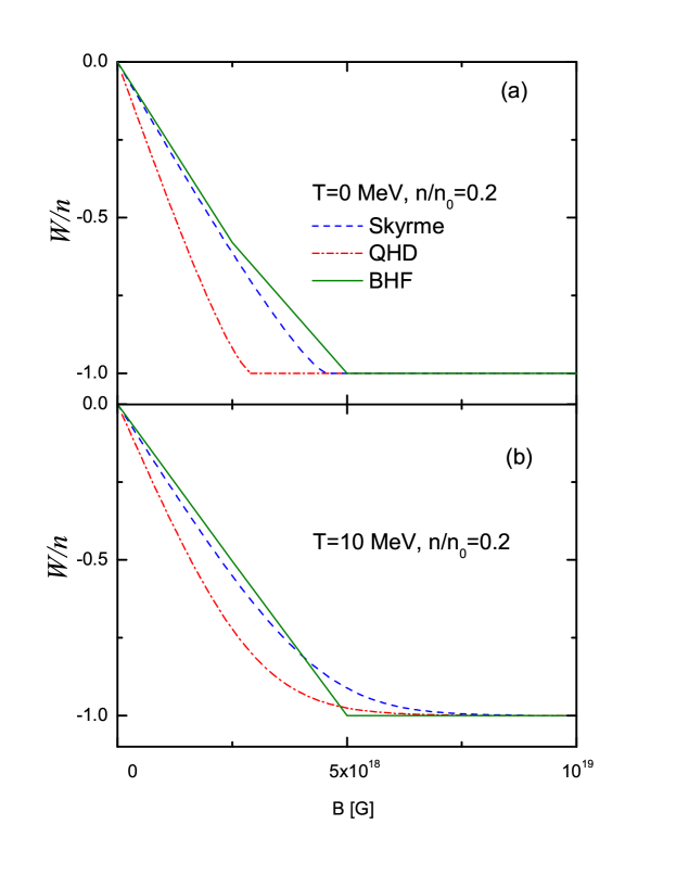
Figure 3: (Color online) Spin asymmetry as a function of the magnetic field intensity for $n/n_{0}=0.2$ and $T=0$ (panel a) and $T=10$ MeV (panel b) for the three models considered. The magnetic filed intensity is given in units of $10^{18}$ G.

A similar description remains valid at higher temperatures (see Figs. 1(b) and 2(b)), but the passage from CPS to PPS becomes softer for QHD and Skyrme. Hence, the definition of a threshold density no longer makes sense for those cases. Additional details can be seen in Fig. 3, where $W/n$ is depicted as a function of $B$ for a fixed density $n/n_{0}=0.2$ and two temperatures. Clearly, for $B=0$, there is no spin asymmetry ($W/n=0$) and the rate at which it changes from this value to a completely polarized configuration ($W/n=-1$), is more pronounced for QHD than for Skyrme, and for Skyrme than for BHF. At $T=0$ a quick change of slope is detected at the transition point. The BHF result keeps this feature still at $T=10$ MeV. At the same temperature, the change from PPS to CPS-D, becomes a soft passage for both QHD and Skyrme. From Figs. 1-3, we see that the temperature-dependence of the spin asymmetry is weaker for BHF than for the other two models.

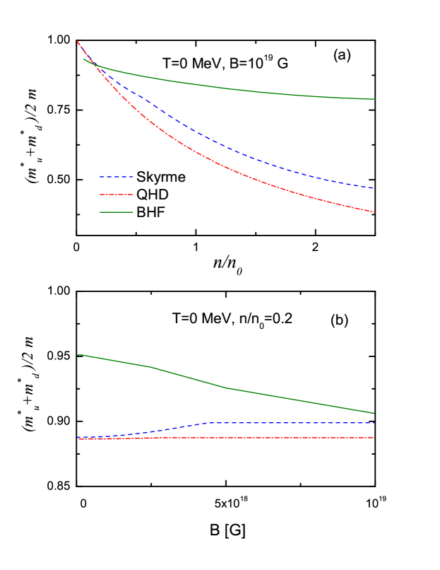
Figure 4: (Color online) Panel a: average effective mass as a function of the density at $T=0$ MeV for $B=10^{19}$G. Panel b: average effective mass as a function of the magnetic field intensity for $n/n_{0}=0.2$ and $T=0$. The magnetic filed intensity is given in units of $10^{18}$ G.

The effects of an external magnetic field on the single-particle properties can have significative consequences, for instance in the transport properties in a dense nuclear medium. We examine in the following the neutron effective mass, which is representative of the single neutron properties. In order to compare fairly the different predictions, we define a spin averaged effective mass $m^{*}=(m^{*}_{\uparrow}+m^{*}_{\downarrow})/2m$ for BHF and Skyrme. It must be taken into account that within the QHD model, $m^{*}$ is a scalar which does not have an explicit dependence on the spin state. Let us also recall that the effective mass has a momentum–dependence in the BHF model and for purposes of comparison we fix $m_{\sigma}^{*}\cong m_{\sigma}^{*}(k_{F_{\sigma}})$, where $k_{F_{\sigma}}$, is the Fermi momentum of neutrons with spin projection $\sigma$. This comparison is presented in Fig. 4, where $m^{*}$ is shown as a function of the density at $T=0$ and $B=10^{19}$ G in Fig. 4(a), and as a function of the magnetic field intensity at $T=0$ and $n/n_{0}=0.2$ in Fig. 4(b). In Fig. 4(a), we found a monotonous decrease over the range of densities studied here. For the QHD and Skyrme models the spin average effective mass decreases approximately to one half of its vacuum value for $n/n_{0}=1.5$, whereas in the BHF case it exhibits a $\sim 20-22\%$ decrease at most. As seen in the lower panel, the effect of the magnetic field on $m^{*}$ is small for all the models at $n/n_{0}=0.2$. In particular, for the QHD model $m^{*}$ is almost constant with $B$, whereas it increases by about $\sim 1-2\%$ for the Skyrme one, and decreases by about $\sim 5\%$ in the BHF case.

We have checked that for higher densities the magnetic effect on $m^{*}$ becomes negligible for both the BHF and QHD models because for these two models (see Figs. 1 and 2) the spin asymmetry $W/n$ goes to zero as density increases, the effect of the magnetic field therefore being less and less important. On the contrary, for the Skyrme model the effect $B$ on $m^{*}$ becomes significative already for densities $n/n_{0}>0.3$, and it is emphasized as the density grows. This is again a consequence of the ferromagnetic instability predicted by the Skyrme model at high densities mentioned before.

We analyze now the effective mass corresponding to different spin polarization states within the non-relativistic potentials. The dependence on the density at $T=0$, depicted in Fig. 5 shows some interesting features. In both cases $m_{\downarrow}^{*}$ is larger than $m_{\uparrow}^{*}$, and the splitting, for a fixed density, increases with $B$. For the BHF model, however, this difference decreases as the density increases, and the two masses cross at $n/n_{0}\sim 2.5$. The reason is that in the BHF case, when density increases, the effect of the magnetic field becomes less important and is completely negligible when the system reaches the nonpolarized state at high densities. On the other hand, the Skyrme model shows a perceptible difference, even for extreme densities, due to the ferromagnetic instability predicted by this model. Furthermore, for densities $n<n_{t}$, $m_{\downarrow}^{*}$ saturates at its vacuum value for Skyrme. This is a consequence of the particular SLy4 parametrization used, for which is $b_{0}+b_{1}=0$ for neutrons with spin down in the CPS-D state (see Eq. (27)).

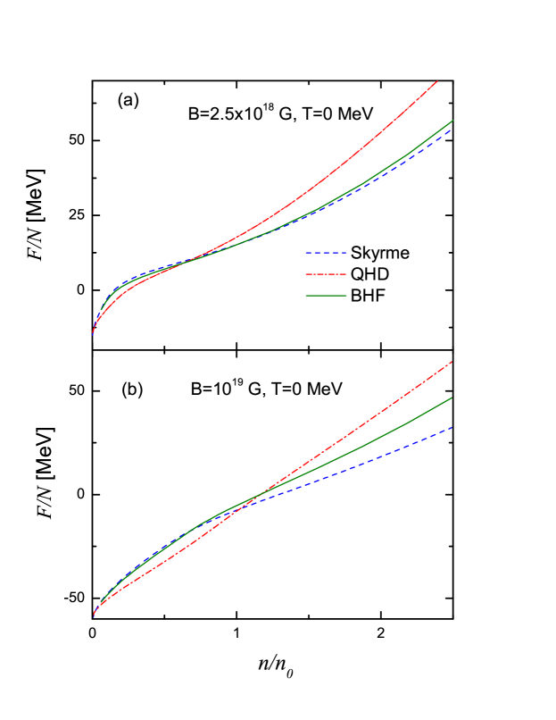
Figure 6: (Color online) Free-energy per particle as a function of the density for $T=0$ MeV and $B=2.5\times 10^{18}$ G (panel a) and $B=10^{19}$ G (panel b).

In the following we discuss some bulk thermodynamical properties. The first one, is the free energy per particle, $F/N={\mathcal{F}}/n$, shown in Fig. 6 as a function of the density for $T=0$ and for two magnetic field intensities. It must be mentioned that, for the sake of comparison, the rest mass contribution was subtracted in the QHD results.

It is a well known fact that neutron matter is not bound by the action of nuclear forces. However, as seen in the figure, the presence of a magnetic field of $\sim 2.5\times 10^{18}$ G leads to a bound state, already at low densities. The binding increases when the strength of the field grows, and for fields $B\sim 10^{19}$ G neutron matter is bound up to saturation density. At relatively low densities the kinetic energy and the repulsion between neutrons are reduced, the effect of the magnetic field becoming the dominant one. For medium and high densities the repulsive character of the neutron-neutron interaction and the kinetic energy dominate over the magnetic field and the system becomes unbound. We note that there is good agreement between BHF and Skyrme for densities up to $n_{0}$.

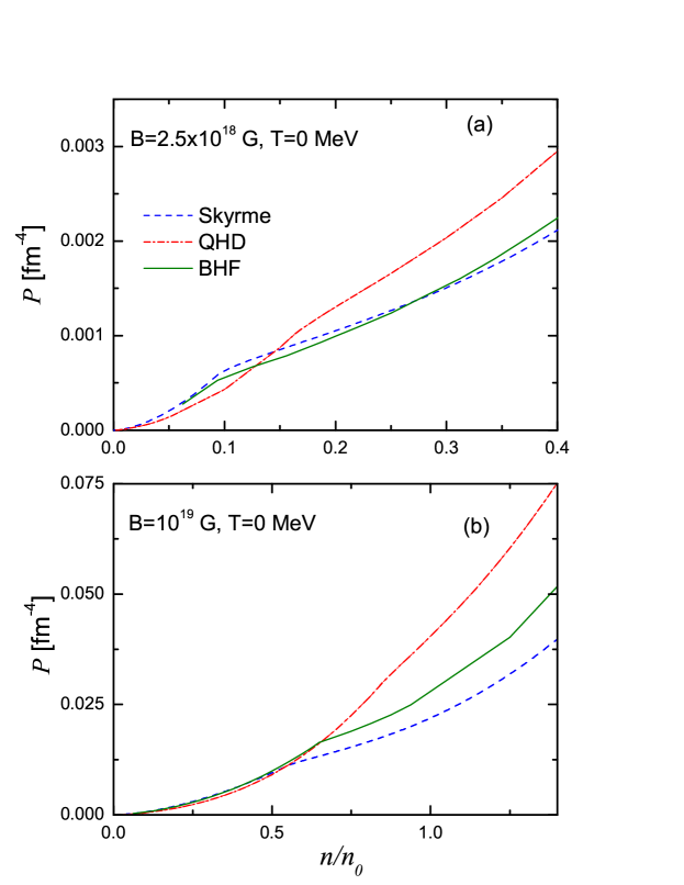
Figure 7: (Color online) Pressure as a function of the density for $T=0$ MeV and $B=2.5\times 10^{18}$ G (panel a) and $B=10^{19}$ G (panel b).

To carry on with the study of some bulk thermodynamical properties, we focus now on the pressure. It is shown as a function of the density for T=0 in Fig. 7, where we have selected a range of densities below the saturation value $n_{0}$ and two magnetic field intensities. As is required by stability conditions the curves show a monotonous increasing behavior. A careful inspection for all the models shows a slight change of slope at the threshold densities $n_{t}$, where the system changes its polarization state from CPS-D to PPS. We have checked that the temperature variation within the range covered in this work has no significative effects on the pressure for any of the models.

Up to this moment we have obtained compatible descriptions of the equation of state, without discontinuities and with some differences in the values of the density where the system changes from CPS-D to PPS. Hence, it is interesting to analyze some of the first derivatives of the thermodynamical potentials. We choose as significative examples the isothermal compressibility $K$, and the magnetic susceptibility $\chi$, as stated in Sec. II.

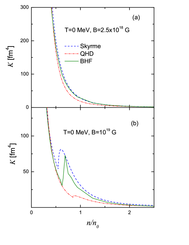
Figure 8: (Color online) Isothermal compressibility as a function of the density for $T=0$ MeV and $B=2.5\times 10^{18}$ G (panel a) and $B=10^{19}$ G (panel b).

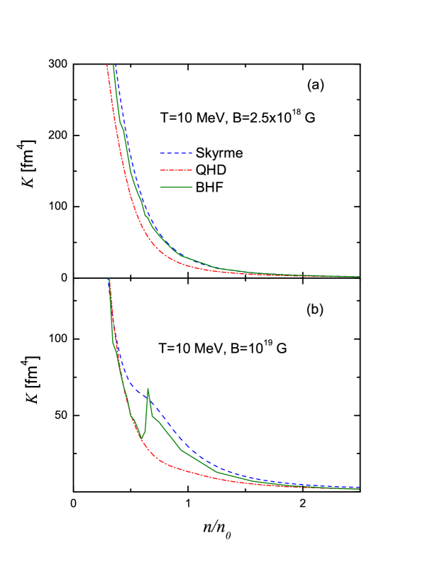
Figure 9: (Color online) Same as Fig. 8 for $T=10$ MeV.

In the first place, we show in Fig. 8 the isothermal compressibility $K$ as a function of the density at zero temperature for $B=2.5\times 10^{18}$ G in Fig. 8(a) and $B=10^{19}$ G in Fig. 8(b). For these magnetic intensities the compressibility falls from relatively high values at very low densities, decreasing monotonously with density until a peak appears at the threshold density $n_{t}$. The origin of this peak is due simply to the change of the slope of the pressure at the threshold density $n_{t}$ (see Fig. 7). Beyond this point, the compressibility behaves in a very similar way for all the models. From the asymptotic behavior exhibited, it can be said that under the hypotheses assumed, neutron matter can be considered incompressible for $n/n_{0}>2$. We note also that for $B=2.5\times 10^{18}$ G the same kind of peaks are present at very low densities but they are not visible on this figure. In Fig. 9 it is shown that thermal effects smear out the peaks within the Skyme and QHD descriptions. Note that the BHF result is almost insensitive to thermal effects, showing a peak similar to that of the zero temperature case.

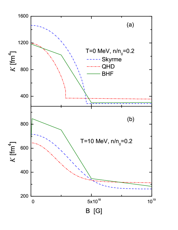
Figure 10: (Color online) Isothermal compressibility as a function of the magnetic field intensity for $n/n_{0}=0.2$ and $T=0$ MeV (panel a) and $T=10$ MeV (panel b). The magnetic filed intensity is given in units of $10^{18}$ G.

The dependence of $K$ on the magnetic field intensity at a fixed density $n/n_{0}=0.2$ is exhibited in Fig. 10. For $T=0$ (Fig. 10(a)) there are two different regimes, in the low field region the compressibility resembles an inverted parabola. For stronger fields, $K$ reaches a plateau with an almost constant value $K\sim 400$ fm⁴. The change of regime takes place at a threshold field intensity $B_{t}$, with an abrupt change of slope. The value of $B_{t}$ depends on the model, the lower one, $B_{t}=2.86\times 10^{18}$ G, corresponds to QHD whereas those of Skyrme and BHF are $B_{t}=4.60\times 10^{18}$ G and $B_{t}=5\times 10^{18}$ G, respectively. The plateau can be easily understood by taking into account that for values of $B>B_{t}$ the system is completely polarized, i.e., $W=-n$, and a further increase of $B$ has no effect on it. Consequently, the value of $K$ remains equal to that at $B=B_{t}$. The increment of temperature (see Fig. 10(b)) seems to erase this abrupt change of slope for the Skyrme and QHD models, whereas the BHF case keeps the angular points still for $T=10$ MeV. In addition, the asymptotic values are smaller than the ones for $T=0$.

Note that the isothermal incompressibility ($K^{-1}$) was studied in Ref. ANG3 , at $T=0$ and relatively low magnetic intensities. Using the SLy7 parametrization of the Skyrme model, a monotonous behavior was found for the low to medium densities regime.

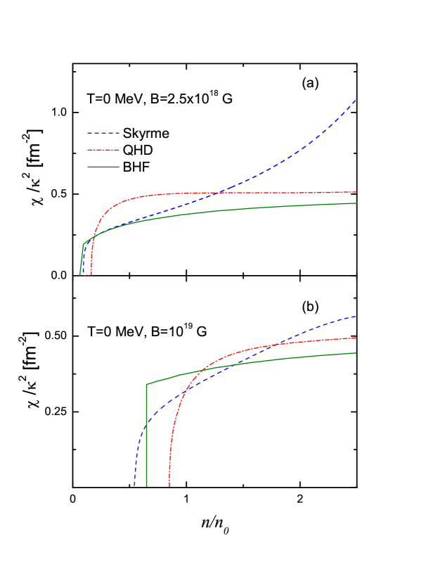
Figure 11: (Color online) Magnetic susceptibility over $\kappa^{2}$ as a function of the density for $T=0$ MeV and $B=2.5\times 10^{18}$ G (panel a) and $B=10^{19}$ G (panel b).

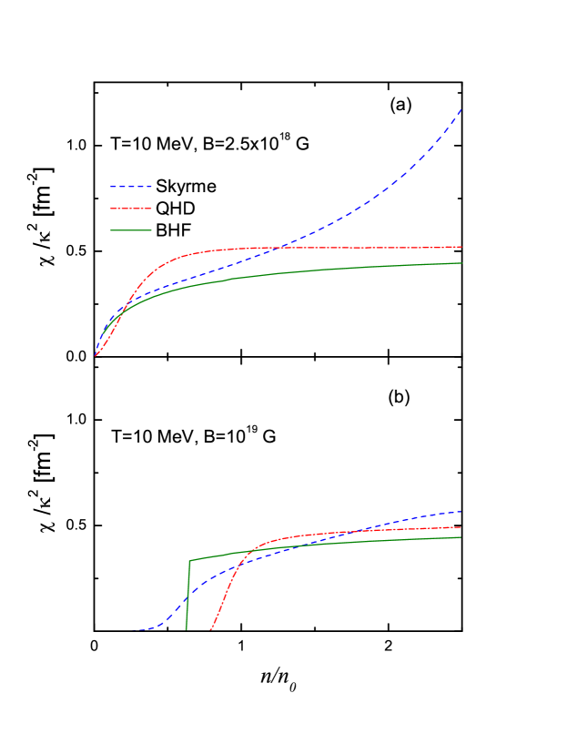
Figure 12: (Color online) Same as Fig. 11 for $T=10$ MeV.

Finally, we analyze the magnetic susceptibility, which is very weak for neutron matter. However, as shown in the following, it provides valuable information about the character of the change of spin polarization. In Fig. 11 the susceptibility is shown as a function of the density for $T=0$ and two values of the magnetic field. For densities smaller than the threshold density $n_{t}$ and zero temperature the magnetization of the system is saturated. Therefore, a further increase of the field intensity does not change the magnetization. Consequently, we have $\chi=0$ for $n<n_{t}$. A sharp increase is detected for densities slightly above $n_{t}$. Beyond that point, $\chi$ shows only moderate variations in the QHD and BHF cases, whereas it grows with an almost constant rate in the Skyrme one. In Fig. 12, we see that thermal effects, as pointed out in similar circumstances discussed in this section, smears out the abrupt changes in the QHD and Skyrme cases while it seems to have a small effect in the BHF one.

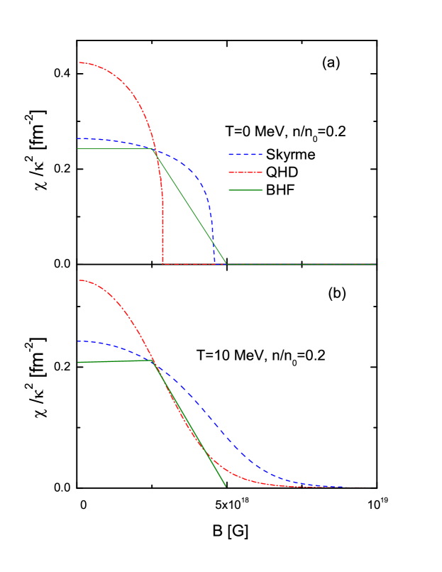
Figure 13: (Color online) Magnetic susceptibility over $\kappa^{2}$ as a function of the magnetic field intensity for $n/n_{0}=0.2$ and $T=0$ MeV (panel a) and $T=10$ MeV (panel b). The magnetic filed intensity is given in units of $10^{18}$ G.

The dependence of $\chi$ on the magnetic intensity is given in Fig. 13. The density is fixed at $n/n_{0}=0.2$ and temperature at $T=0$ (Fig. 13(a)) and $T=10$ MeV (Fig. 13(b)). A description similar to that given for Fig. 10 holds here. As in that case, the same threshold value $B_{t}$ separates, in each model, the high intensity field regime, where $\chi/\kappa^{2}\simeq 0$, from the monotonous decreasing trend found for the low field domain. Since the susceptibility measures the rate of change of the magnetization with the applied field, it is clear that as the system saturates spin in the CPS-D state, the susceptibility goes to zero. This fact explains, as in the case of $K$, the plateau exhibited by $\chi$ for $B>B_{t}$.

IV Conclusions

In the present work we have analyzed the behavior of neutron matter in the presence of an external magnetic field for a wide range of densities, two temperatures and several magnetic field intensities. Magnetic effects are small due to the smallness of the intrinsic magnetic moment of the neutron. However, we have found that there are some observables that give a clear signal of a change in the physical configuration of the system in the low density-low temperature regime. In order to give a discussion as general as possible, we have used different models of the nuclear interaction. All of them have been successfully used in different fields of the nuclear physics, although they have very different theoretical foundations. They are: i) the Brueckner–Hartree–Fock (BHF) approach using the Argonne V18 nucleon-nucleon potential supplemented with the Urbana IX three-nucleon force, ii) the covariant formulation known as Quantum Hadro-dynamics (QHD) in its FSU-Gold version within a mean field approach, and iii) the SLy4 parametrization of the non-relativistic Skyrme effective potential in a Hartree-Fock scheme.

The spin asymmetry $W$ is a key feature to understand the behavior of the system. The results for $W$ obtained by the different models are in qualitative agreement. Within the range of magnetic field intensities considered here, the system is completely polarized for small densities up to a threshold density $n_{t}$, where it changes into a partially polarized state. The value of $n_{t}$ increases with the magnetic field intensity. There are some details, such as the location of $n_{t}$, which differ from one model to the other. However, they can be understood in terms of the in-medium nuclear interaction. Thermal effects tend to soften the passage from completely to partially polarized and reduce the degree of polarization.

We have studied the effective mass due to its importance in the single-particle properties. We have found that it is a monotonous decreasing function of the density for the three models. We have seen that the effect of the magnetic field on $m^{*}$ is in general small for all the models at low densities, becoming completely negligible at high densities for the BHF and QHD models whereas, on the contrary, for the Skyrme force it becomes more important as density grows. This is a consequence of the well known ferromagnetic instability predicted by these forces.

With regard to the equation of state, there are not significative differences among the various predictions and only weak clues about the change of polarization. The second derivatives of the thermodynamical potentials, such as the compressibility and the magnetic susceptibility, give clear evidence of a change in the system. At zero temperature they show an abrupt change of regime that becomes diffuse as the temperature is increased in the QHD and Skyrme cases. The isothermal compressibility, for example, has a non-monotonous behavior around the threshold density $n_{t}$. This feature can have significative consequences as, for instance, in the propagation of density waves through the crust of neutron stars.

In conclusion, we have found robust results supported by the three models. The change in the global polarization of the system does not produce discontinuities in the thermodynamical potentials. The remarkable change of the slope found in the equation of state at the threshold point resembles a second order phase transition. However, a detailed examination of the relevant second order derivatives of the thermodynamic potential does not show any discontinuity. Hence, we conclude the system undergoes a continuous passage or experiences a higher order phase transition. The consequences of the non-monotonous behavior of the compressibility near the transition point requires further investigation.

To establish significative differences among the three models within the subject under study, additional information must be taken into account. We can mention here the cooling rate of a neutron star, which strongly depends on the magnetization state of matter. In ANG2 it was shown that there is a decrease of the neutrino opacity of magnetized matter with respect to the non-magnetized case. Of course, a realistic description of this issue requires some refinements, such as the inclusion of protons, leptons, and exotic degrees of freedom such as hyperons in $\beta$-equilibrium. This would be the natural extension of the present work and will be considered in a near future. However, we believe that a good understanding of the simpler neutron matter case is the first step in such direction.

Figure 5: (Color online) Neutron up and neutron down effective masses as a function of the density for $T=0$ MeV and $B=2.5\times 10^{18}$ G (panel a) and $B=10^{19}$ G (panel b). Results are shown only for the BHF and Skyrme models.

References

- (1) D. Lai, Rev. Mod. Phys. 73 (2001) 629.
- (2) J. M. Lattimer and M. Prakash, Phys. Rep. 442, 109 (2007).
- (3) Y. A. Shibanov and D. G. Yakovlev, Astron. Astrophys. 309, 171 (1996).
- (4) D. G. Yakovlev, A. D. Kaminker, O. Y. Gnedin, and P. Haensel, Phys. Rep. 442, 1 (2001) and references therein.
- (5) V. G. Bezchastnov and P. Haensel, Phys. Rev. D 54, 3706 (1996); D. A. Baiko and D. G. Yakovlev, Astron. Astrophys. 342, 192 (1999); D. Chandra, A. Goyal, and K. Goswami, Phys. Rev. D 65, 053003 (2002).
- (6) D. H. Brownell and J. Callaway, Nuovo Cimento B 60, 169 (1969).
- (7) M. J. Rice, Phys. Lett. A 29, 637 (1969).
- (8) J. W. Clark and N. C. Chao, Lett. Nuovo Cimento, 2, 185 (1969).
- (9) J. W. Clark, Phys. Rev. Lett. 23, 1463 (1969).
- (10) S. D. Silvertein, Phys. Rev. Lett. 23, 139 (1969).
- (11) E. Østgaard, Nucl. Phys. A 154, 202 (1970).
- (12) J. M. Pearson, G. Saunier, Phys. Rev. Lett. 24, 325 (1970).
- (13) V. R. Pandharipande, V. K. Garde, J. K. Srivastava, Phys. Lett. B 38, 485 (1972).
- (14) S. O. Bäckman and C. G. Källman, Phys, Lett. B 43, 263 (1973).
- (15) P. Haensel, Phys. Rev. C 11, 1822 (1975).
- (16) A. D. Jackson, E. Krotscheck, D. E. Meltzer, and R. A. Smith, Nucl. Phys. A 386, 125 (1982).
- (17) M. Kutschera and W. Wójcik, Phys. Lett. B 223, 11 (1989); Phys. Lett. B 325 , 271 (1994).
- (18) S. Marcos, R. Niembro, M. L. Quelle, and J. Navarro, Phys. Lett. B 271, 277 (1991); P. Bernardos, S. Marcos, R. Niembro and M. L.. Quelle, Phys. Lett. B 356, 175 (1996).
- (19) A. Vidaurre, J. Navarro, and J. Bernabeu, Astron. Astrophys. 135, 361 (1984); A. Rios, A. Polls and I. Vidaña, Phys. Rev. C 71, 055802 (2005).
- (20) A. Rios, A. Polls and I. Vidaña, Phys. Rev. C 71, 055802 (2005).
- (21) D. López-Val, A. Rios, A. Polls, and I. Vidaña, Phys. Rev. C 74, 068801 (2006).
- (22) S. Fantoni, A. Sarsa, and K. E. Schmidt, Phys. Rev. Lett. 87, 181101 (2001).
- (23) I. Vidaña, A. Polls, and A. Ramos, Phys. Rev. C 65, 035804 (2002).
- (24) I. Vidaña and I. Bombaci, Phys. Rev. C 66, 045801 (2002).
- (25) I. Bombaci, A. Polls, A. Ramos, A. Rios, and I. Vidaña, Phys. Lett. B 632, 638 (2006).
- (26) F. Sammarruca and P. G. Krastev, Phys. Rev. C 75, 034315 (2007).
- (27) F. Sammarruca, Phys. Rev. C 83, 064304 (2011).
- (28) M. Bigdeli Phys. Rev. C 82 054312 (2010).
- (29) J. Margueron and H. Sagawa, J. Phys. G: Nucl. Part. Phys. 36, 125102 (2009).
- (30) N. Chamel, S. Goriely, and J. M. Pearson, Phys. Rev. C 80, 065804 (2009).
-
(31)
D. Kharzeev, Phys. Lett. B 633, 260 (2006);
D. E. Kharzeev, L. D. McLerran, H. J. Warringa, Nucl. Phys. A 803, 227 (2008). - (32) Y.-J. Mo, S.-Q. Feng, and Y.-F. Shi, Phys. Rev. C 88, 024901 (2013).
- (33) V. V. Skokov, A. Yu. Illarionov, and V. D. Toneev, Int. J. Mod. Phys. A 24, 5925 (2009).
- (34) S. Chakrabarty, D. Bandhyopadhyay, and S. Pal, Phys. Rev. Lett. 78, 2898 (1997).
- (35) A. Broderick, M. Prakash, and J. M. Lattimer, Astroph. J. 537, 351 (2000).
- (36) P. Yue and H. Shen, Phys. Rev. C 79, 025803 (2009).
- (37) M. Sinha, B. Mukhopadhyay, and A. Sedrakian, Nucl. Phys. A 898, 43 (2013); M. Sinha and D. Bandyopadhay, Phys. Rev. D 79, 123001 (2009).
- (38) A. Rabhi, C. Providência, and J. Da Providência, Phys. Rev. C 79, 015804 (2009).
- (39) A. Rabhi, C. Providência, and J. Da Providência, Phys. Rev. C 80, 025806 (2009).
- (40) C.-Y. Ryu, M.-K. Cheoun, T. Kajino, T. Maruyama, and G.J. Mathews, Astropart. Phys. 38, 25 (2012).
- (41) C. Y. Ryu, K. S. Kim, and M.-K. Cheoun, Phys. Rev. C 82, 025804 (2010).
- (42) A. Rabhi, P. K. Panda, and C. Providência, Phys. Rev. C 84, 035803 (2011).
- (43) M. A. Pérez-García, C. Providência, and A. Rabhi, Phys. Rev. C 84, 045803 (2011).
- (44) J. Dong, W. Zuo, and J. Gu, Phys. Rev. D 87 103010 (2013).
- (45) J. P. W. Diener and F. G. Scholtz, Phys. Rev. C 87, 065805 (2013).
- (46) J. Dong, U. Lombardo, W. Zuo, and H. Zhang, Nucl. Phys. A 898, 32 (2013).
- (47) M. A. Perez Garcia, Phys. Rev. C 77, 065806 (2008).
- (48) A. A. Isayev, Phys. Rev. C 74, 057301 (2006); A. A. Isaev and J. Yang, Phys. Rev. C 80, 065801 (2009)
- (49) R. Aguirre, Phys. Rev. C 83, 064314 (2012); R. Aguirre and E. Bauer, Phys. Lett. B 721, 136 (2013).
- (50) G. H. Bordbar and Z. Rezaei, Phys. Lett. B 718, 1125 (2012).
- (51) M. Bigdeli, Phys. Rev. C 85, 034302 (2012).
- (52) S. Gandolfi, F. Pederiva, S. Fantoni, and K. E. Schmidt, Phys. Rev. Lett. 98, 102503 (2007); S. Gandolfi, A. Y. Illarionov, K. E. Schmidt, F. Pederiva, and S. Fantoni, Phys. Rev. C 79, 054005 (2009).
- (53) J. P. Jekeune, A. Lejeune, and C. Mahaux, Phys. Rep. 25, 83 (1976).
- (54) H. Q. Song, M. Baldo, G. Giansiracusa, and U. Lombardo, Phys. Rev. Lett. 81, 1584 (1998); Phys. Lett. B 411, 237 (1999).
- (55) R. B. Wiringa, V. G. J. Stoks, and R. Schiavilla, Phys. Rev. C 51, 38 (1995).
- (56) B. S. Pudliner, V. R. Pandharipande, J. Carlson, and R. B. Wiringa, Phys. Rev. Lett. 74, 4396 (1995).
- (57) B. A. Loiseau, Y. Nogami, and C. K. Ross, Nucl. Phys. A 165, 601 (1971); 176, 665 (E) (1971); P. Grangé, M. Martzolff, Y. Nogami, D. W. L. Sprung, and C. K. Ross, Phys. Lett B 60 273 (1976).
- (58) M. Baldo and L. Ferreira, Phys. Rev. C 59, 682 (1999).
- (59) B. G. Todd-Rutel and J. Piekarewicz, Phys. Rev. Lett. 95, 122501 (2005).
- (60) D. Vautherin, and D. M. Brink, Phys. Rev. C 3, 626 (1972); P. Quentin, and H. Flocard, Annu. Rev. Nucl. Part. Sci. 28, 523 (1978).
- (61) F. Douchin, P. Haensel, and J. Meyer, Nucl. Phys. A 665, 419 (2000).
- (62) M. A. Pérez-García, J. Navarro, and A. Polls, Phys. Rev. C 80, 025802 (2009).
- (63) M. A. Pérez-García, Phys. Rev. C 80, 045804 (2009).