LMU-ASC 82/13

Resolving Witten’s Superstring Field Theory

Theodore Erler, Sebastian Konopka, Ivo Sachs

Arnold Sommerfeld Center, Ludwig-Maxmillians University,
Theresienstrasse 37, D-80333, Munich, Germany

Abstract

We regulate Witten’s open superstring field theory by replacing the picture-changing insertion at the midpoint with a contour integral of picture changing insertions over the half-string overlaps of the cubic vertex. The resulting product between string fields is non-associative, but we provide a solution to the $A_{\infty}$ relations defining all higher vertices. The result is an explicit covariant superstring field theory which by construction satisfies the classical BV master equation.

1 Introduction

For the bosonic string, the construction of covariant string field theories is more-or-less well understood. We know how to construct an action, quantize it, and prove that the vertices and propagators cover the the moduli space of Riemann surfaces relevant for computing amplitudes. For the superstring this kind of understanding is largely absent. A canonical formulation of open superstring field theory was provided by Berkovits [1, 2], but it utilizes the “large” Hilbert space which obscures the relation to supermoduli space. Moreover, quantization of the Berkovits theory is not completely understood [3, 4, 5, 6]. Motivated by this problem, we seek a different formulation of open superstring field theory satisfying three criteria:

(1) The kinetic term is diagonal in mode number.

(2) Gauge invariance follows from the same algebraic structures which ensure gauge invariance in open bosonic string field theory.

(3) The vertices do not require integration over bosonic moduli.

We assume $(1)$ since we want the theory to have a simple propagator. We assume $(2)$ since we want to be able to quantize the theory in a straightforward manner, following the work of Thorn [7], Zwiebach [8] and others for the bosonic string. Finally we assume $(3)$ for simplicity, but also because we would like to know whether open string field theory can describe closed string physics through its quantum corrections. Once we add stubs to the open string vertices, the nature of the minimal area problem changes and requires separate degrees of freedom for closed strings at the quantum level [9].

Condition $(1)$ rules out the modified cubic theory and its variants [10, 11, 12, 13, 14, 15], and $(2)$ rules out the Berkovits theory. This leaves the original proposal for open superstring field theory at picture $-1$, described by Witten [16]. The problem is that this theory is singular and incomplete. A picture changing operator in the cubic term leads to a divergence in the four point amplitude which requires subtraction against a divergent quartic vertex [17]. Likely an infinite number of divergent higher vertices are needed to ensure gauge invariance, but have never been constructed.

In this paper we would like to complete the construction of Witten’s open superstring field theory in the NS sector. We achieve this by resolving the singularity in the cubic vertex by spreading the picture changing insertion away from the midpoint. As a result the product is non-associative. But we know how to formulate a gauge invariant action with a non-associative product [19]. The action takes the form

$$S=\frac{1}{2}\omega(\Psi,Q\Psi)+\frac{1}{3}\omega(\Psi,M_{2}(\Psi,\Psi))+\frac{1}{4}\omega(\Psi,M_{3}(\Psi,\Psi,\Psi))+...\ ,$$ (1.1)

where $\omega$ is the symplectic bilinear form and $Q,M_{2},M_{3},...$ are multi-string products which satisfy the relations of an $A_{\infty}$ algebra. The fact that one can in principle construct a regularization of Witten’s theory along these lines is well-known. The new ingredient we provide is an exact solution of the $A_{\infty}$ relations, giving an explicit and computable definition of the vertices to all orders.

The resulting theory is quite simple. However, its explicit form depends on a choice of BPZ even charge of the picture changing operator

$$X=\oint\frac{dz}{2\pi i}f(z)X(z),$$ (1.2)

which tells us how to spread the picture changing insertion in the cubic vertex away from the midpoint. As far as we know, there is no canonical way to make this choice. This suggests the result of a partial gauge fixing; in fact, a gauge fixed version of Berkovits’ theory resembling our approach has been explored by Iimori, Noumi, Okawa, and Torii [20, 21]. Our regularization of the cubic vertex is inspired by their work.

This paper is organized as follows. In section 2 we review Witten’s superstring field theory up to cubic order and describe our regularization of the cubic vertex. In section 3 we compute the quartic vertex by requiring that the BRST variation of the 3-product cancel against the non-associativity of the 2-product. For this purpose it is useful to treat the picture changing operator $X$ as BRST exact in the large Hilbert space. Then it is no longer guaranteed that the 3-product will be independent of the $\xi$ zero mode. We determine a BRST exact correction which ensures that the 3-product is in the small Hilbert space. On the way, we find it useful to introduce some additional multi-string products which play a central role in the recursion defining higher vertices. In section 4 we review some mathematical apparatus which relates multi-string products to coderivations on the tensor algebra, and use this language to streamline the computation of the quartic vertex and then the quintic vertex. In section 5 we derive a set of recursive equations which determine multi-string products to all orders. In section 6 we show that the four-point amplitude derived from our theory agrees with the first quantized result. We end with some discussion.

2 Witten’s Theory up to Cubic order

The string field $\Psi$ is a Grassmann odd, ghost number $1$ and picture number $-1$ state in the boundary superconformal field theory of an open superstring quantized in a reference D-brane background. $\Psi$ is in the small Hilbert space, meaning it is independent of the zero mode of the $\xi$ ghost obtained upon bosonization of the $\beta\gamma$ system [22], or, equivalently, it is annihilated by the zero mode of the $\eta$ ghost,

$$\eta\Psi=0,$$ (2.1)

where $\eta\equiv\eta_{0}$. The linear field equation is

$$Q\Psi=0,$$ (2.2)

where $Q\equiv Q_{B}$ is the worldsheet BRST operator. At picture $-1$, we can express on-shell states in Siegel gauge

$$\Psi\sim ce^{-\phi}\mathcal{O}^{\mathrm{m}}(0),$$ (2.3)

where $\mathcal{O}^{\mathrm{m}}$ is a superconformal matter primary of dimension $1/2$.

Let’s explain a few sign conventions which are common in discussions of $A_{\infty}$ algebras, but are otherwise nonstandard in most discussions of open string field theory. Given a string field $A$ with Grassmann parity $\epsilon(A)$, we define its “degree”

$$\mathrm{deg}(A)\equiv\epsilon(A)+1\ \mathrm{mod}\ \mathbb{Z}_{2}.$$ (2.4)

The dynamical field $\Psi$ has even degree, though it corresponds to a Grassmann odd vertex operator. We also define a $2$-product and symplectic form:

$$m_{2}(A,B)\!\!\!\!\!\!\!\! \equiv(-1)^{\mathrm{deg}(A)}A*B,$$ (2.5)

$$\omega(A,B)\!\!\!\!\!\!\!\! \equiv(-1)^{\mathrm{deg}(A)}\langle A,B\rangle.$$ (2.6)

The 2-product is essentially the same as Witten’s open string star product except for the sign. Likewise, the symplectic form is essentially the same as the BPZ inner product except for the sign. The main advantage of these sign conventions is that all multi-string products have the same (odd) degree as the BRST operator $Q$. In particular, $m_{2}$ adds one unit of degree when multiplying string fields:

$$\mathrm{deg}(m_{2}(A,B))=\mathrm{deg}(A)+\mathrm{deg}(B)+1.$$ (2.7)

These conventions slightly change the appearance of the familiar Chern-Simons axioms. The derivation property of $Q$ and the associativity of the star product take the form:

$$0\!\!\!\!\!\!\!\! =Q^{2}A,$$

$$0\!\!\!\!\!\!\!\! =Qm_{2}(A,B)+m_{2}(QA,B)+(-1)^{\mathrm{deg}(A)}m_{2}(A,QB),$$

$$0\!\!\!\!\!\!\!\! =m_{2}(m_{2}(A,B),C)+(-1)^{\mathrm{deg}(A)}m_{2}(A,m_{2}(B,C)).$$ (2.8)

Rephrased in the appropriate language (to be described later), these relations can be understood as the statement that $Q$ and $m_{2}$ are nilpotent and anticommute. Finally, the symplectic form is BRST invariant

$$0=\omega(QA,B)+(-1)^{\mathrm{deg}(A)}\omega(A,QB),$$ (2.9)

and satisfies

$$\omega(A,B)=-(-1)^{\mathrm{deg}(A)\mathrm{deg}(B)}\omega(B,A),$$ (2.10)

and so is (graded) antisymmetric.

Now let’s discuss Witten’s superstring field theory. Expanding the action up to cubic order gives

$$S=\frac{1}{2}\omega(\Psi,Q\Psi)+\frac{1}{3}\omega(\Psi,M_{2}(\Psi,\Psi))+...\ .$$ (2.11)

The 2-product $M_{2}$ above is different from the open string star product $m_{2}$. In particular, the total picture must be $-2$ to obtain a nonvanishing correlator on the disk, so the 2-product $M_{2}(A,B)$ must have picture $+1$. The original proposal of Witten [16] was to define $M_{2}$ using the open string star product with an insertion of the picture changing operator $X(z)=Q\cdot\xi(z)$ at the open string midpoint. Specifically, taking the sign inherited from (2.5),

$$M_{2}(A,B)=X(i)m_{2}(A,B).$$ (2.12)

The problem is that repeated $M_{2}$-products are divergent due to a double pole in the $X$-$X$ OPE. This leads to a breakdown in gauge invariance and a divergence in the 4-point amplitude [17]. To avoid these problems we will make a more general ansatz:

$$M_{2}(A,B)\equiv\frac{1}{3}\Big{[}Xm_{2}(A,B)+m_{2}(XA,B)+m_{2}(A,XB)\Big{]},$$ (2.13)

where $X$ is a BPZ even charge of the picture changing operator:

$$X=\oint_{|z|=1}\frac{dz}{2\pi i}f(z)X(z).$$ (2.14)

The product $M_{2}$ now explicitly depends on a choice of 1-form $f(z)$, which describes how the picture changing is spread over the half-string overlaps of the Witten vertex. Provided $f(z)$ is holomorphic in some nondegenerate annulus around the unit circle, products of $X$ with itself are regular, and in particular the $4$-point amplitude is finite. Note that the geometry of the cubic vertex (2.13) is the same as in Witten’s open bosonic string field theory. This means that the propagator together with the cubic vertex already cover the bosonic moduli space of Riemann surfaces with boundary [23]. Therefore higher vertices must be contact interactions without integration over bosonic moduli.

Since $X$ is BPZ even, the 1-form $f(z)$ satisfies

$$f(z)=-\frac{1}{z^{2}}f\left(-\frac{1}{z}\right).$$ (2.15)

We also assume

$$\oint_{|z|=1}\frac{dz}{2\pi i}f(z)=1,$$ (2.16)

since any other number could be absorbed into a redefinition of the open string coupling constant. Perhaps the simplest choice of $X$ is the zero mode of the picture changing operator:

$$X_{0}=\oint_{|z|=1}\frac{dz}{2\pi i}\frac{1}{z}X(z).$$ (2.17)

If we like, we can also choose $X$ so that it approaches Witten’s singular midpoint insertion as a limit. For example we can take

$$f(z)=\frac{1}{z-i\lambda}-\frac{1}{z-\frac{i}{\lambda}},$$ (2.18)

which as $\lambda\to 1^{-}$ approaches a delta function localizing $X$ at the midpoint. Note that the annulus of analyticity,

$$\lambda<|z|<\frac{1}{\lambda},$$ (2.19)

degenerates to zero thickness in the $\lambda\to 1^{-}$ limit. This is why Witten’s original vertex produces contact divergences.

3 Quartic Order

The action constructed so far is not gauge invariant because the 2-product $M_{2}$ is not associative:

$$M_{2}(M_{2}(A,B),C)+(-1)^{\mathrm{deg}(A)}M_{2}(A,M_{2}(B,C))\neq 0.$$ (3.1)

To restore gauge invariance we search for a 3-product $M_{3}$, a 4-product $M_{4}$, and so on so that the full set of multilinear maps satisfy the relations of an $A_{\infty}$ algebra. Using these multilinear maps to define higher vertices, the action

$$S=\frac{1}{2}\omega(\Psi,Q\Psi)+\sum_{n=2}^{\infty}\frac{1}{n+1}\omega(\Psi,M_{n}(\underbrace{\Psi,...,\Psi}_{n\ \mathrm{times}}))$$ (3.2)

is gauge invariant by construction. We offer a proof in appendix A.

Figure 3.1: Pictorial representation of the associator of $M_{2}$. We can take the numbers $1,2,3$ to represent the states which are multiplied, and $4$ to represent the output of the associator. The “T” shape represents a contour integral of $X$ surrounding the respective Witten vertex, and two factors of $\frac{1}{3}$ comes from the two vertices.

As a first step we construct the 3-product $M_{3}$ which defines the quartic vertex. The first two $A_{\infty}$ relations say that $Q$ is nilpotent and a derivation of the 2-product $M_{2}$. The third relation characterizes the failure of $M_{2}$ to associate in terms of the BRST variation of $M_{3}$:

$$0\!\!\!\!\!\!\!\! =M_{2}(M_{2}(A,B),C)+(-1)^{\mathrm{deg}(A)}M_{2}(A,M_{2}(B,C))+QM_{3}(A,B,C)$$

$$\ \ \ +M_{3}(QA,B,C)+(-1)^{\mathrm{deg}(A)}M_{3}(A,QB,C)+(-1)^{\mathrm{deg}(A)+\mathrm{deg}(B)}M_{3}(A,B,QC).$$

The last four terms represent the BRST variation of $M_{3}$ by placing a $Q$ on each output of the quartic vertex. To visualize how to solve for $M_{3}$, consider figure 3.1, which gives a schematic worldsheet picture the configuration of $X$ contour integrals in the $M_{2}$ associator. To pull a $Q$ off of the $X$ contours, it would clearly help if $X$ were a BRST exact quantity. In the large Hilbert space it is, since we can write

$$X=[Q,\xi],\ \ \ \ \ \ \ \ \xi\equiv\oint_{|z|=1}\frac{dz}{2\pi i}f(z)\xi(z),$$ (3.4)

where $\xi$ is the charge of the $\xi$-ghost defined by the 1-form $f(z)$. Now pulling a $Q$ out of the associator simply requires replacing one of the $X$ contours in each term with a $\xi$ contour. Since there are two $X$ contours in each term, there are two ways to do this, and by cyclicity we should sum both ways and divide by two. This is shown in figure 3.2. Translating this picture into an equation gives a solution for $M_{3}$:

$$M_{3}(A,B,C)\!\!\!\!\!\!\!\! =\frac{1}{2}\Big{[}M_{2}(A,\overline{M}_{2}(B,C))-(-1)^{\mathrm{deg}(A)}\overline{M}_{2}(A,M_{2}(B,C))$$ (3.5)

$$\ \ \ +M_{2}(\overline{M}_{2}(A,B),C)-\overline{M}_{2}(M_{2}(A,B),C)\Big{]}+Q\text{-exact},$$

where we leave open the possibility of adding a $Q$-exact piece (which would not contribute to the associator). $\overline{M}_{2}$ in this equation is a new object that we call the dressed-2-product:

$$\overline{M}_{2}(A,B)\equiv\frac{1}{3}\Big{[}\xi m_{2}(A,B)-m_{2}(\xi A,B)-(-1)^{\mathrm{deg}(A)}m_{2}(A,\xi B)\Big{]}.$$ (3.6)

This is essentially the same as $M_{2}$, only the $X$ contour has been replaced by a $\xi$ contour. The dressed-2-product has even degree, and as required its BRST variation is $M_{2}$:

$$M_{2}(A,B)=Q\overline{M}_{2}(A,B)-\overline{M}_{2}(QA,B)-(-1)^{\mathrm{deg}(A)}\overline{M}_{2}(A,QB).$$ (3.7)

Acting $\eta$ on $\overline{M}_{2}$ gives yet another object which we call the bare-2-product:

$$m_{2}(A,B)=\eta\overline{M}_{2}(A,B)-\overline{M}_{2}(\eta A,B)-(-1)^{\mathrm{deg}{A}}\overline{M}_{2}(A,\eta B).$$ (3.8)

The bare-2-product has odd degree. As it happens the bare-2-product is the same as Witten’s open string star product (with the sign of (2.5)). Both the dressed-product and the bare-product will have nontrivial higher-point generalizations.

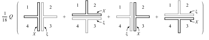
Figure 3.2: Pictorial representation of the associator as a BRST exact quantity. The black “T” shape represents a contour integral of $X$ around the Witten vertex and the grey “T” shape represents the corresponding contour integral of $\xi$. We have four terms since we require the quartic vertex to be cyclic.

So far the construction of the 3-product has seemed easy, essentially because we have allowed ourselves to treat the 2-product as BRST exact. But if the 2-product were “truly” BRST exact, then we would expect our theory to produce a trivial $S$-matrix—in other words, it would be a complicated nonlinear rewriting of a free theory. A useful analogy to this situation is finding the first nonlinear correction to an infinitesimal gauge transformation. While this might be straightforward, usually constructing pure gauge solutions is not physically interesting. What makes our construction nontrivial is that the “gauge transformation” generating the cubic and quartic vertex lives in the large Hilbert space. And the result of the gauge transformation must be in the small Hilbert space. This suggests a structural analogy to solving the equations of motion of Berkovits superstring field theory. We will clarify the meaning of this analogy in appendix C.

This raises a central point: While we can introduce $\xi$ into our calculations as a formal convenience, consistency requires that all multilinear maps defining string vertices must be in the small Hilbert space. This is already true for $M_{2}$, but not yet true for $M_{3}$. For this reason we make use of our freedom to add a BRST exact piece in (3.5)

$$Q\text{-exact}\!\!\!\!\!\!\!\! =\frac{1}{2}\Big{[}Q\overline{M}_{3}(A,B,C)-\overline{M}_{3}(QA,B,C)-(-1)^{\mathrm{deg}(A)}\overline{M}_{3}(A,QB,C)$$ (3.9)

$$\ \ \ \ \ \ \ \ \ -(-1)^{\mathrm{deg}(A)+\mathrm{deg}(B)}\overline{M}_{3}(A,B,QC)\Big{]},$$

where $\overline{M}_{3}$ will be defined in such a way as to ensure that the total 3-product is in the small Hilbert space. The object $\overline{M}_{3}$ will be called the dressed-3-product. Now we require that $M_{3}$ is in the small Hilbert space:

$$0=\eta M_{3}(A,B,C)\!\!\!\!\!\!\!\! =\frac{1}{2}\Big{[}-(-1)^{\mathrm{deg}(A)}M_{2}(A,m_{2}(B,C))-(-1)^{\mathrm{deg}(A)}m_{2}(A,M_{2}(B,C))$$ (3.10)

$$\ \ \ -M_{2}(m_{2}(A,B),C)-m_{2}(M_{2}(A,B),C)\Big{]}+\eta(Q\text{-exact}).$$

To avoid writing too many terms, we assume $A,B,C$ are in the small Hilbert space and the $Q$-exact piece is as in (3.9). With some algebra this simplifies to

$$0=\eta M_{3}(A,B,C)\!\!\!\!\!\!\!\! =-\frac{1}{3}\Big{[}(-1)^{\mathrm{deg}(A)}m_{2}(A,Xm_{2}(B,C))+m_{2}(Xm_{2}(A,B),C)\Big{]}$$ (3.11)

$$\ \ \ +\eta(Q\text{-exact}).$$

We now pull an overall $Q$ out of this equation. This replaces the $X$ insertion in the first two terms with a $\xi$ insertion:

$$\eta M_{3}(A,B,C)\!\!\!\!\!\!\!\! =Q\left(\frac{1}{3}\Big{[}m_{2}(A,\xi m_{2}(B,C))+m_{2}(\xi m_{2}(A,B),C)\Big{]}-\frac{1}{2}\eta\overline{M}_{3}(A,B,C)\right)$$ (3.12)

$$\ \ \ +\mathrm{other\ terms},$$

where “other terms” take a similar form but with $Q$ acting on one of the three other external states. Since $\eta M_{3}$ should be zero, it is reasonable to assume that the dressed-3-product $\overline{M}_{3}$ should satisfy

$$\eta\overline{M}_{3}(A,B,C)\!\!\!\!\!\!\!\! =\frac{2}{3}\Big{[}m_{2}(A,\xi m_{2}(B,C))+m_{2}(\xi m_{2}(A,B),C)\Big{]}$$ (3.13)

$$\equiv m_{3}(A,B,C).$$

The right hand side defines what we call the bare-3-product, $m_{3}$. Of course, this equation is consistent only if the bare-3-product happens to be in the small Hilbert space. It is: Acting $\eta$ on $m_{3}$ gives the $m_{2}$ associator, which vanishes. Though equation (3.13) does not uniquely determine $\overline{M}_{3}$, there is a natural solution: take $m_{3}$ and place a $\xi$ on each external state:

$$\overline{M}_{3}\!\!\!\!\!\!\!\! \equiv\frac{1}{4}\Big{[}\xi m_{3}(A,B,C)-m_{3}(\xi A,B,C)-(-1)^{\mathrm{deg}(A)}m_{3}(A,\xi B,C)$$ (3.14)

$$\ \ \ \ \ \ -(-1)^{\mathrm{deg}(A)+\mathrm{deg}(B)}m_{3}(A,B,\xi C)\Big{]}.$$

Thus the dressed-3-product is described by a configuration of $\xi$ contours shown in figure 3.3. This gives an explicit definition of the quartic vertex in the small Hilbert space consistent with gauge invariance.

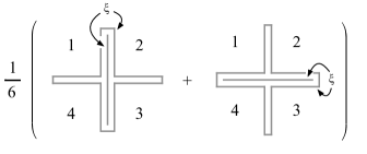
Figure 3.3: Schematic picture of the $\xi$ contours defining the dressed-3-product. The vertical and horizontal lines inside the cross represents an insertion of $\xi$ between open string star products. The cross represents a sum of $\xi$ insertions acting on all external states.

4 Quintic Order

Performing all substitutions, the final expression for $M_{3}$ involves some 30 terms with various combinations of $m_{2}$s, $X$s and $\xi$s acting on external states. At higher orders the vertices become even more complicated, and we need more economical notation. Therefore we explain a few conceptual and notational devices which are common in more mathematical discussions of $A_{\infty}$ algebras. See for example [24] and references therein. Then we revisit the derivation of the quartic vertex, and continue on to the quintic vertex.

We are interested in multilinear maps taking $n$ copies of the BCFT state space $\mathcal{H}$ into one copy. Such a map can be viewed as a linear operator from the $n$-fold tensor product of $\mathcal{H}$ into $\mathcal{H}$:

$$b_{n}:\mathcal{H}^{\otimes n}\to\mathcal{H}.$$ (4.1)

Suppose we have a state in $\mathcal{H}^{\otimes n}$ of the form

$$\Psi_{1}\otimes\Psi_{2}\otimes...\otimes\Psi_{n}\in\mathcal{H}^{\otimes n},$$ (4.2)

then $b_{n}$ acts on such a state as

$$b_{n}(\Psi_{1}\otimes\Psi_{2}\otimes...\otimes\Psi_{n})=b_{n}(\Psi_{1},\Psi_{2},...,\Psi_{n}),$$ (4.3)

where the right hand side is the multilinear map as denoted in previous sections. Since we can use the states (4.2) to form a basis, (4.3) defines the action of $b_{n}$ on the whole tensor product space.

Given $b_{n}$, define the following linear operator on $\mathcal{H}^{\otimes N\geq n}$:

$$\mathbb{I}^{\otimes N-n-k}\otimes b_{n}\otimes\mathbb{I}^{\otimes k}:\mathcal{H}^{\otimes N}\to\mathcal{H}^{\otimes N-n+1}.$$ (4.4)

It acts on states of the form (4.2) as

$$\mathbb{I}^{\otimes N-n-k}\otimes b_{n}\otimes\mathbb{I}^{\otimes k}(\Psi_{1}\otimes\Psi_{2}\otimes...\otimes\Psi_{N})=$$

$$\ \ \ \ \ \ (-1)^{\mathrm{deg}(b_{n})(\mathrm{deg}(\Psi_{1})+...+\mathrm{deg}(\Psi_{N-n-k}))}\times$$

$$\ \ \ \ \ \ \ \ \ \ \ \ \Psi_{1}\otimes...\otimes\Psi_{N-n-k}\otimes b_{n}(\Psi_{N-n-k+1},...,\Psi_{N-k})\otimes\Psi_{N-k+1}\otimes...\otimes\Psi_{N}.$$ (4.5)

It acts in the obvious way: It leaves the tensor product of the first $N-n+k$ states untouched, multiplies the next $n$ states, and leaves the tensor product of remaining $k$ states untouched. It also may produce a sign from commuting $b_{n}$ past the first $N-n-k$ states.

With these ingredients we can define a natural action of $b_{n}$ or the tensor algebra:

$$T\mathcal{H}=\mathcal{H}^{\otimes 0}\,\oplus\,\mathcal{H}\,\oplus\,\mathcal{H}^{\otimes 2}\,\oplus\,\mathcal{H}^{\otimes 3}\,\oplus\,...\ .$$ (4.6)

In this context we will denote the action of $b_{n}$ with a boldface ${\bf b}_{n}$:

$${\bf b}_{n}:T\mathcal{H}\to T\mathcal{H}.$$ (4.7)

${\bf b}_{n}$ acts on the tensor algebra as a so-called coderivation. We define ${\bf b}_{n}$ as follows: On the $\mathcal{H}^{\otimes N\geq n}$ component of the tensor algebra, we take

$${\bf b}_{n}\Psi\equiv\sum_{k=0}^{N-n}\mathbb{I}^{\otimes N-n-k}\otimes b_{n}\otimes\mathbb{I}^{\otimes k}\Psi,\ \ \ \ \Psi\in\mathcal{H}^{\otimes N\geq n}\subset T\mathcal{H},$$ (4.10)

and on the $\mathcal{H}^{\otimes N<n}$ component, we take ${\bf b}_{n}$ to vanish. Naturally, on the $\mathcal{H}^{\otimes n}$ component, ${\bf b}_{n}=b_{n}$. So the coderivation ${\bf b}_{n}$ and multilinear map $b_{n}$ are isomorphic.

The advantage of this language is that it gives us a natural notion of “multiplication” between multilinear maps. We just compose the corresponding coderivations. Particularly important are (graded) commutators of coderivations. With a little algebra, we can show that the commutator of two coderivations ${\bf b}_{m},{\bf b}_{n}^{\prime}$ derived from the maps

$$b_{m}:\mathcal{H}^{\otimes m}\to\mathcal{H},$$

$$b_{n}^{\prime}:\mathcal{H}^{\otimes n}\to\mathcal{H},$$ (4.11)

is a coderivation $[{\bf b}_{m},{\bf b}_{n}^{\prime}]$ derived from the map

$$[b_{m},b_{n}^{\prime}]:\mathcal{H}^{m+n-1}\to\mathcal{H},$$ (4.12)

with

$$[b_{m},b_{n}^{\prime}]\equiv b_{m}\sum_{k=0}^{m-1}\mathbb{I}^{\otimes m-1-k}\otimes b^{\prime}_{n}\otimes\mathbb{I}^{k}-(-1)^{\mathrm{deg}(b_{m})\mathrm{deg}(b_{m}^{\prime})}b_{n}^{\prime}\sum_{k=0}^{n-1}\mathbb{I}^{\otimes n-1-k}\otimes b_{m}\otimes\mathbb{I}^{k}.$$ (4.13)

The sums in this equation are closely related to the multitude of terms which appear in formulas for the 3-product. This notation allows us to keep track of these terms in a very economical fashion.

Consider for example the first three $A_{\infty}$ relations:

$$0\!\!\!\!\!\!\!\! =Q^{2}A,$$ (4.14)

$$0\!\!\!\!\!\!\!\! =QM_{2}(A,B)+M_{2}(QA,B)+(-1)^{\mathrm{deg}(A)}M_{2}(A,QB),$$ (4.15)

$$0\!\!\!\!\!\!\!\! =M_{2}(M_{2}(A,B),C)+(-1)^{\mathrm{deg}(A)}M_{2}(A,M_{2}(B,C))+QM_{3}(A,B,C)$$

$$\ \ \ +M_{3}(QA,B,C)+(-1)^{\mathrm{deg}(A)}M_{3}(A,QB,C)+(-1)^{\mathrm{deg}(A)+\mathrm{deg}(B)}M_{3}(A,B,QC).$$

Recalling (4.3), we can “factor out” the string fields $A,B,C$:

$$0\!\!\!\!\!\!\!\! =Q^{2},$$ (4.17)

$$0\!\!\!\!\!\!\!\! =QM_{2}+M_{2}(Q\otimes\mathbb{I}+\mathbb{I}\otimes Q),$$ (4.18)

$$0\!\!\!\!\!\!\!\! =M_{2}(M_{2}\otimes\mathbb{I}+\mathbb{I}\otimes M_{2})+QM_{3}+M_{3}(Q\otimes\mathbb{I}\otimes\mathbb{I}+\mathbb{I}\otimes Q\otimes\mathbb{I}+\mathbb{I}\otimes\mathbb{I}\otimes Q),$$

Now from (4.13) we recognize these terms as commutators of coderivations. The first three $A_{\infty}$ relations reduce to

$$0\!\!\!\!\!\!\!\! =\frac{1}{2}[{\bf Q},{\bf Q}],$$ (4.20)

$$0\!\!\!\!\!\!\!\! =[{\bf Q},{\bf M}_{2}],$$ (4.21)

$$0\!\!\!\!\!\!\!\! =[{\bf Q},{\bf M}_{3}]+\frac{1}{2}[{\bf M}_{2},{\bf M}_{2}].$$ (4.22)

Now let’s return to the quartic vertex. The 2-product and dressed-2-product are defined

$$M_{2}\!\!\!\!\!\!\!\! \equiv\frac{1}{3}\Big{(}Xm_{2}+m_{2}(X\otimes\mathbb{I}+\mathbb{I}\otimes X)\Big{)},$$ (4.23)

$$\overline{M}_{2}\!\!\!\!\!\!\!\! \equiv\frac{1}{3}\Big{(}\xi m_{2}-m_{2}(\xi\otimes\mathbb{I}+\mathbb{I}\otimes\xi)\Big{)},$$ (4.24)

and satisfy

$${\bf M}_{2}=[{\bf Q},\overline{\bf M}_{2}],$$ (4.25)

$${\bf m}_{2}=[{\bm{\eta}},\overline{\bf M}_{2}],$$ (4.26)

where ${\bf m}_{2}$ is the bare-2-product. Following (3.5), the 3-product is expressed

$${\bf M}_{3}=\frac{1}{2}\Big{(}[{\bf Q},\overline{\bf M}_{3}]+[{\bf M}_{2},\overline{\bf M}_{2}]\Big{)}.$$ (4.27)

where $\overline{\bf M}_{3}$ is the dressed-3-product. Now its easy to plug into (4.22) and check the relevant $A_{\infty}$ relation. Taking the commutator with ${\bf Q}$ the first term in (4.27) drops out since $[{\bf Q},{\bf Q}]=0$. Using the Jacobi identity the second term gives $-\frac{1}{2}[{\bf M}_{2},{\bf M}_{2}]$, which cancels against the $\frac{1}{2}[{\bf M}_{2},{\bf M}_{2}]$ term in (4.22).

Now we need to make sure ${\bf M}_{3}$ is in the small Hilbert space. Acting with ${\bm{\eta}}$ we find

$$0=[{\bm{\eta}},{\bf M}_{3}]\!\!\!\!\!\!\!\! =\frac{1}{2}\Big{(}-[{\bf Q},[{\bm{\eta}},\overline{\bf M}_{3}]]-[{\bf M}_{2},{\bf m}_{2}]\Big{)},$$ (4.28)

$$=\frac{1}{2}\Big{(}-[{\bf Q},[{\bm{\eta}},\overline{\bf M}_{3}]]-[[{\bf Q},\overline{\bf M}_{2}],{\bf m}_{2}]\Big{)},$$

$$=\frac{1}{2}\big{[}{\bf Q},-[{\bm{\eta}},\overline{\bf M}_{3}]+[{\bf m}_{2},\overline{\bf M}_{2}]\big{]}.$$

Since this should vanish, we assume

$$[{\bm{\eta}},\overline{\bf M}_{3}]={\bf m}_{3}\equiv[{\bf m}_{2},\overline{\bf M}_{2}],$$ (4.29)

where ${\bf m}_{3}$ is the bare-3-product. This is consistent since ${\bf m}_{3}$ is in the small Hilbert space:

$$[{\bm{\eta}},{\bf m}_{3}]=-[{\bf m}_{2},{\bf m}_{2}]=0,$$ (4.30)

where we used associativity of ${\bf m}_{2}$. Thus we can define the dressed-3-product by placing a $\xi$ on each output of the bare-3-product:

$$\overline{M}_{3}=\frac{1}{4}\Big{(}\xi m_{3}-m_{3}(\xi\otimes\mathbb{I}\otimes\mathbb{I}+\mathbb{I}\otimes\xi\otimes\mathbb{I}+\mathbb{I}\otimes\mathbb{I}\otimes\xi)\Big{)}.$$ (4.31)

Via (4.27), this completely determines the four vertex.

Now we claim that a similar procedure extends to higher orders. Just to see it work in the next example, let’s construct the quintic vertex. The relevant $A_{\infty}$ relation is

$$0=[{\bf Q},{\bf M}_{4}]+[{\bf M}_{2},{\bf M}_{3}].$$ (4.32)

The solution is

$${\bf M}_{4}=\frac{1}{3}\Big{(}[{\bf Q},\overline{\bf M}_{4}]+[{\bf M}_{2},\overline{\bf M}_{3}]+[{\bf M}_{3},\overline{\bf M}_{2}]\Big{)},$$ (4.33)

where $\overline{\bf M}_{4}$ is the dressed-4-product. To check, compute:

$$[{\bf Q},{\bf M}_{4}]\!\!\!\!\!\!\!\! =\frac{1}{3}\Big{(}-[{\bf M}_{2},[{\bf Q},\overline{\bf M}_{3}]]+[[{\bf Q},{\bf M}_{3}],\overline{\bf M}_{2}]-[{\bf M}_{3},{\bf M}_{2}]\Big{)},$$ (4.34)

$$=\frac{1}{3}\Big{(}-\big{[}{\bf M}_{2},2{\bf M}_{3}-[{\bf M}_{2},\overline{\bf M}_{2}]\big{]}+\big{[}-{\textstyle\frac{1}{2}}[{\bf M}_{2},{\bf M}_{2}],\overline{\bf M}_{2}\big{]}-[{\bf M}_{3},{\bf M}_{2}]\Big{)},$$

$$=\frac{1}{3}\Big{(}-2[{\bf M}_{2},{\bf M}_{3}]+[{\bf M}_{2},[{\bf M}_{2},\overline{\bf M}_{2}]]-[{\bf M}_{2},[{\bf M}_{2},\overline{\bf M}_{2}]]-[{\bf M}_{2},{\bf M}_{2}]\Big{)},$$

$$=\frac{1}{3}\Big{(}-3[{\bf M}_{2},{\bf M}_{3}]\Big{)},$$

$$=-[{\bf M}_{2},{\bf M}_{3}].$$

In the first step we used the Jacobi identity and $[{\bf Q},{\bf Q}]=0$, $[{\bf Q},{\bf M}_{2}]=0$ and $[{\bf Q},\overline{\bf M}_{2}]={\bf M}_{2}$. In the second step we used the $A_{\infty}$ relation for ${\bf M}_{3}$ and used (4.27) to solve for $[{\bf Q},\overline{\bf M}_{3}]$. The remaining steps use the Jacobi identity. Since we want ${\bf M}_{4}$ to be in the small Hilbert space we demand

$$0=[{\bm{\eta}},{\bf M}_{4}]\!\!\!\!\!\!\!\! =\frac{1}{3}\Big{(}-[{\bf Q},[{\bm{\eta}},\overline{\bf M}_{4}]]-[{\bf M}_{2},{\bf m}_{3}]-[{\bf M}_{3},{\bf m}_{2}]\Big{)},$$ (4.35)

$$=\frac{1}{3}\left(-[{\bf Q},[{\bm{\eta}},\overline{\bf M}_{4}]]-[{\bf M}_{2},{\bf m}_{3}]-\frac{1}{2}\big{[}[{\bf Q},\overline{\bf M}_{3}]+[{\bf M}_{2},\overline{\bf M}_{2}],{\bf m}_{2}\big{]}\right),$$

$$=\frac{1}{3}\left(-[{\bf Q},[{\bm{\eta}},\overline{\bf M}_{4}]]-[{\bf M}_{2},{\bf m}_{3}]-\frac{1}{2}[[{\bf M}_{2},{\bf m}_{2}],\overline{\bf M}_{2}]+\frac{1}{2}[{\bf M}_{2},[{\bf m}_{2},\overline{\bf M}_{2}]]+\frac{1}{2}[{\bf Q},[{\bf m}_{2},\overline{\bf M}_{3}]]\right),$$

$$=\frac{1}{3}\left(-[{\bf Q},[{\bm{\eta}},\overline{\bf M}_{4}]]-\frac{1}{2}[{\bf m}_{3},{\bf M}_{2}]+\frac{1}{2}[[{\bf Q},{\bf m}_{3}],\overline{\bf M}_{2}]+\frac{1}{2}[{\bf Q},[{\bf m}_{2},\overline{\bf M}_{3}]]\right),$$

$$=\frac{1}{3}\left[{\bf Q},\left(-[{\bm{\eta}},\overline{\bf M}_{4}]+\frac{1}{2}[{\bf m}_{3},\overline{\bf M}_{2}]+\frac{1}{2}[{\bf m}_{2},\overline{\bf M}_{3}]\right)\right].$$

In the second equation we substituted (4.27) in place of ${\bf M}_{3}$. In the third we used the Jacobi identity. In the fourth we substituted the definition of ${\bf m}_{3}$, and in the fifth we pulled out a ${\bf Q}$. Since this should vanish, we assume

$$[{\bm{\eta}},\overline{\bf M}_{4}]={\bf m}_{4}\equiv\frac{1}{2}\Big{(}[{\bf m}_{3},\overline{\bf M}_{2}]+[{\bf m}_{2},\overline{\bf M}_{3}]\Big{)},$$ (4.36)

where ${\bf m}_{4}$ is the bare-4-product. Consistently, ${\bf m}_{4}$ is in the small Hilbert space:

$$[{\bm{\eta}},{\bf m}_{4}]\!\!\!\!\!\!\!\! =[{\bf m}_{3},{\bf m}_{2}],$$ (4.37)

$$=[[{\bf m}_{2},\overline{\bf M}_{2}],{\bf m}_{2}],$$

$$=[[{\bf m}_{2},{\bf m}_{2}],\overline{\bf M}_{2}]-[[{\bf m}_{2},\overline{\bf M}_{2}],{\bf m}_{2}],$$

$$=[[{\bf m}_{2},{\bf m}_{2}],\overline{\bf M}_{2}]-[{\bm{\eta}},{\bf m}_{4}].$$

$$=0$$

Therefore the dressed-4-product can be constructed by placing a $\xi$ on each output of $m_{4}$:

$$\overline{M}_{4}=\frac{1}{5}\Big{(}\xi m_{4}-m_{4}(\xi\otimes\mathbb{I}\otimes\mathbb{I}\otimes\mathbb{I}+\mathbb{I}\otimes\xi\otimes\mathbb{I}\otimes\mathbb{I}+\mathbb{I}\otimes\mathbb{I}\otimes\xi\otimes\mathbb{I}+\mathbb{I}\otimes\mathbb{I}\otimes\mathbb{I}\otimes\xi)\Big{)}.$$ (4.38)

This completely fixes the theory up to quintic order.

5 Witten’s Theory to All Orders

Now we are ready to discuss the construction of vertices to all orders. The $n$-th $A_{\infty}$ relation reads

$$0=[{\bf M}_{n},{\bf M}_{1}]+[{\bf M}_{n-1},{\bf M}_{2}]+...+[{\bf M}_{2},{\bf M}_{n-1}]+[{\bf M}_{1},{\bf M}_{n}],$$ (5.1)

where ${\bf M}_{1}\equiv{\bf Q}$. To express all such relations in a compact form, it is useful to introduce a generating function ${\bf M}(t)$:

$${\bf M}(t)\equiv\sum_{n=0}^{\infty}t^{n}{\bf M}_{n+1},$$ (5.2)

where $t$ is some parameter. Then the full set of $A_{\infty}$ relations is equivalent to the equation

$$[{\bf M}(t),{\bf M}(t)]=0.$$ (5.3)

The $n$th relation is found by expanding this equation in a power series and reading off the coefficient of $t^{n-1}$.

The solution we’re after takes the form

$${\bf M}_{n+2}=\frac{1}{n+1}\sum_{k=0}^{n}[{\bf M}_{n-k+1},\overline{\bf M}_{k+2}].$$ (5.4)

If we know the products up to ${\bf M}_{n+1}$, and the dressed-products up to $\overline{\bf M}_{n+2}$, this equation determines the next product ${\bf M}_{n+2}$. The proof is as follows. Define a generating function for the dressed-products:

$$\overline{\bf M}(t)=\sum_{n=0}^{\infty}t^{n}\overline{\bf M}_{n+2}$$ (5.5)

Then the recursive formula (5.4) follows from the $t^{n}$ component of the differential equation

$$\frac{d}{dt}{\bf M}(t)=[{\bf M}(t),\overline{\bf M}(t)].$$ (5.6)

This equation implies

$$\frac{d}{dt}[{\bf M}(t),{\bf M}(t)]=2[[{\bf M}(t),{\bf M}(t)],\overline{\bf M}(t)].$$ (5.7)

Let

$$[{\bf M}(t),{\bf M}(t)]_{n+1}=\sum_{k=0}^{n}[{\bf M}_{n-k+1},{\bf M}_{k+1}],$$ (5.8)

be the combination of ${\bf M}$s appearing in the $n+1$st $A_{\infty}$ relation, or equivalently the coefficient of $t^{n}$ in the power series expansion of $[{\bf M}(t),{\bf M}(t)]$. Then equation (5.7) implies a recursive formula for these coefficients:

$$[{\bf M}(t),{\bf M}(t)]_{n+2}=\frac{2}{n+1}\sum_{k=0}^{n}[[{\bf M}(t),{\bf M}(t)]_{n-k+1},\overline{\bf M}_{k+2}].$$ (5.9)

If $[{\bf M}(t),{\bf M}(t)]_{k}$ vanishes for $1\leq k\leq n+1$, then this formula implies that it must vanish for $k=n+2$. So all we have to do is show that $[{\bf M}(t),{\bf M}(t)]_{k}$ vanishes for $k=1$. It does because

$$[{\bf M}(t),{\bf M}(t)]_{1}=[{\bf Q},{\bf Q}]=0.$$ (5.10)

This completes the proof that (5.4) implies the $A_{\infty}$ relations.

Next consider the bare-products ${\bf m}_{n}$. For the moment we will ignore the possible identification between ${\bf m}_{n}$ and $[{\bm{\eta}},\overline{\bf M}_{n}]$. Rather, we will define the bare-products in terms of the recursive formula

$${\bf m}_{n+3}=\frac{1}{n+1}\sum_{k=0}^{n}[{\bf m}_{n-k+2},\overline{\bf M}_{k+2}].$$ (5.11)

If we know the bare-products up to ${\bf m}_{n+2}$ and the dressed-products up to $\overline{\bf M}_{n+2}$, this determines the next bare-product ${\bf m}_{n+3}$. We can check that this formula matches our previous calculation of the bare-3-product and bare-4-product. Suppose that we define a generating function for the bare-products

$${\bf m}(t)=\sum_{n=0}^{\infty}t^{n}{\bf m}_{n+2}.$$ (5.12)

Then (5.11) implies the differential equation

$$\frac{d}{dt}{\bf m}(t)=[{\bf m}(t),\overline{\bf M}(t)].$$ (5.13)

Using a similar argument as just given below (5.7), we can prove

$$[{\bf m}(t),{\bf m}(t)]\!\!\!\!\!\!\!\! =0,$$ (5.14)

$$\ [{\bf m}(t),{\bf M}(t)]\!\!\!\!\!\!\!\! =0$$ (5.15)

recursively from the identities $[{\bf m}_{2},{\bf m}_{2}]=0$ and $[{\bf m}_{2},{\bf Q}]=0$. In components of $t^{n}$,

$$\sum_{k=0}^{n}[{\bf m}_{n-k+2},{\bf m}_{k+2}]\!\!\!\!\!\!\!\! =0,$$ (5.16)

$$\sum_{k=0}^{n}[{\bf m}_{n-k+2},{\bf M}_{k+1}]\!\!\!\!\!\!\!\! =0.$$ (5.17)

This means that the products and bare-products form a pair of mutually commuting $A_{\infty}$ algebras.

This much is true regardless of our choice of dressed-products $\overline{\bf M}_{k}$. What fixes $\overline{\bf M}_{k}$ is the additional condition

$$[{\bm{\eta}},\overline{\bf M}_{k+2}]={\bf m}_{k+2}.$$ (5.18)

We construct a solution to this condition recursively as follows. First note that $[\eta,\overline{\bf M}_{2}]={\bf m}_{2}$ by definition. Second, suppose that we have constructed a solution to (5.18) up to ${\bf m}_{n+2}$ and $\overline{\bf M}_{n+2}$. Then it follows that the bare-product ${\bf m}_{n+3}$ is in the small Hilbert space:

$$[{\bm{\eta}},{\bf m}_{n+3}]=-\frac{1}{n+1}\sum_{k=0}^{n}[{\bf m}_{n-k+2},{\bf m}_{k+2}]=0,$$ (5.19)

where we used the recursive equation (5.11) and the $A_{\infty}$ relations (5.16). Now define the $n+3$rd dressed-product:

$$\overline{M}_{n+3}\equiv\frac{1}{n+4}\left(\xi m_{n+3}-m_{n+3}\sum_{k=0}^{n+2}\mathbb{I}^{\otimes n+2-k}\otimes\xi\otimes\mathbb{I}^{\otimes k}\right).$$ (5.20)

Since ${\bf m}_{n+3}$ is in the small Hilbert space, this implies

$$\ [{\bm{\eta}},\overline{\bf M}_{n+3}]={\bf m}_{n+3}.$$ (5.21)

Proceeding this way inductively, we find a solution to (5.18) for all $k$.

Next we have to show how this construction implies that all products defining vertices are in the small Hilbert space. Acting ${\bm{\eta}}$ on the differential equation (5.6) for ${\bf M}$ gives

$$\frac{d}{dt}[{\bm{\eta}},{\bf M}(t)]\!\!\!\!\!\!\!\! =[[{\bm{\eta}},{\bf M}(t)],\overline{\bf M}(t)]-[{\bf M}(t),{\bf m}(t)],$$ (5.22)

$$=[[{\bm{\eta}},{\bf M}(t)],\overline{\bf M}(t)],$$

where we used (5.18) and the fact that the $A_{\infty}$ algebras of ${\bf M}$ and ${\bf m}$ commute. The $t^{n}$ component of this differential equation implies the recursive formula

$$[{\bm{\eta}},{\bf M}_{n+2}]=\frac{1}{n+1}\sum_{k=0}^{n}[[{\bm{\eta}},{\bf M}_{n-k+1}],\overline{\bf M}_{k+2}].$$ (5.23)

Note that ${\bf M}_{1}={\bf Q}$ commutes with $\eta$. And this equation implies that if all of the products up to ${\bf M}_{n+1}$ are in the small Hilbert space, the next product ${\bf M}_{n+2}$ is also in the small Hilbert space. Thus we have a complete solution of the $A_{\infty}$ relations defining Witten’s superstring field theory.

Figure 5.1: General pattern of recursion defining all higher products. At any stage, we always start with the bare-product and proceed to derive the dressed-product. Next, we can either find the “true” product that defines the vertex, or proceed to the next bare-product and start the process over.

The construction we have provided is recursive. Suppose we have determined all products, bare-products, and dressed-products up to ${\bf M}_{n},{\bf m}_{n}$ and $\overline{\bf M}_{n}$. To proceed to the next order, first we construct the $n+1$st bare-product ${\bf m}_{n+1}$ from equation (5.11). Next we construct the $n+1$st dressed-product $\overline{\bf M}_{n+1}$ from equation (5.20). Finally, using $\overline{\bf M}_{n+1}$ we construct the $n+1$st product ${\bf M}_{n+1}$ via (5.4), or we can proceed to the next order and compute the $n+2$nd bare-product ${\bf m}_{n+2}$, starting the process over. The general pattern of recursion is illustrated in figure 5.1.

Our solution to the $A_{\infty}$ relations depends on the following assumptions:

(1) $Q$ and $\eta$ are nilpotent and anticommute.

(2) $Q$ and $\eta$ are derivations of the product $m_{2}$.

(3) $\eta$ has a homotopy $\xi$ satisfying $[\eta,\xi]=1$.

(4) $m_{2}$ is associative.

Within the context of these assumptions we can construct a slightly more general solution by adding an $\eta$ closed piece to $\xi$. This can have the effect of replacing $X$ in the cubic vertex with a slightly more general operator. Aside from this, perhaps the most interesting assumption to drop is associativity of $m_{2}$. This might be useful, for example, for constructing a theory based on a cubic vertex with worldsheet strips attached to each output, as is done in open-closed bosonic string field theory [9].

The solution of the $A_{\infty}$ relations is not unique. The non-uniqueness can be characterized by our freedom to add an $\eta$ closed piece to $\overline{\bf M}_{n}$ at each order. Perhaps the most nontrivial aspect of our construction is that despite this non-uniqueness we were able to find a natural definition of each vertex, without having to make additional choices at each order. In other words, we found a way to “fix the gauge.”

6 Four-point Amplitudes

It is interesting to see how our regularization of Witten’s theory reproduces the familiar first-quantized scattering amplitudes. Here we focus on the generic four-point amplitude. The general case can probably be treated in a similar fashion.

We start with the color-ordered 4-point amplitude expressed in the form:

$$A_{4}^{{1\mathrm{st}}}(\Psi_{1},\Psi_{2},\Psi_{3},\Psi_{4})=-\int_{0}^{1}dt\Big{\langle}\Big{(}X_{0}\cdot\Psi_{1}(0)\Big{)}\Big{(}b_{-1}X_{0}\cdot\Psi_{2}(t)\Big{)}\Psi_{3}(1)\,\Psi_{4}(\infty)\Big{\rangle}_{UHP}.$$ (6.1)

Here $\Psi_{1},..,\Psi_{4}$ are on-shell vertex operators in the $-1$ picture, and the correlator is evaluated in the small Hilbert space on the upper half plane. We denote the amplitude with the superscript “1st” to indicate that this is the first quantized amplitude, not (yet) the string field theory result. As far as bosonic moduli are concerned, this amplitude is structurally the same as in the bosonic string, and following [25] we can reexpress it using the open string star product and the Siegel gauge propagator in the $s$- and $t$-channels:

$$\!\!\!\!\!\!\!\!\!\!A_{4}^{{1\mathrm{st}}}(\Psi_{1},\Psi_{2},\Psi_{3},\Psi_{4})=$$

$$\!\!\!\!\!-\omega\left(X_{0}\Psi_{1},m_{2}\left(X_{0}\Psi_{2},\frac{b_{0}}{L_{0}}m_{2}(\Psi_{3},\Psi_{4})\right)\right)-\omega\left(X_{0}\Psi_{1},m_{2}\left(\frac{b_{0}}{L_{0}}m_{2}(X_{0}\Psi_{2},\Psi_{3}),\Psi_{4}\right)\right).$$

(6.2)

This is the form of the amplitude we want to compare with Witten’s superstring field theory.

Now consider the 4-point amplitude derived from the Lagrangian:

$$\!\!\!\!\!\!\!\!\!\!\!\!\!A_{4}(\Psi_{1},\Psi_{2},\Psi_{3},\Psi_{4})=$$

$$\!\!\!-\omega\left(\Psi_{1},M_{2}\left(\Psi_{2},\frac{b_{0}}{L_{0}}M_{2}(\Psi_{3},\Psi_{4})\right)\right)-\omega\left(\Psi_{1},M_{2}\left(\frac{b_{0}}{L_{0}}M_{2}(\Psi_{2},\Psi_{3}),\Psi_{4}\right)\right)$$

$$\!\!\!+\omega\Big{(}\Psi_{1},M_{3}(\Psi_{2},\Psi_{3},\Psi_{4})\Big{)}.$$ (6.3)

The amplitude can be viewed as a multilinear map from the four-fold tensor product of the physical state space into complex numbers

$$\langle A_{4}|:\mathcal{H}_{Q}^{\otimes 4}\to\mathbb{C},$$ (6.4)

where $\mathcal{H}_{Q}\subset\mathcal{H}$ is the subspace of states annihilated by $Q$. Pulling $\Psi_{1},...,\Psi_{4}$ off to the right we can then express the amplitude

$$\langle A_{4}|=\langle\omega|\left(\mathbb{I}\otimes M_{2}\left(-\mathbb{I}\otimes\frac{b_{0}}{L_{0}}M_{2}-\frac{b_{0}}{L_{0}}M_{2}\otimes\mathbb{I}\right)+\mathbb{I}\otimes M_{3}\right),$$ (6.5)

where $\langle\omega|:\mathcal{H}^{\otimes 2}\to\mathbb{C}$ is the symplectic form. We can write this using the coderivations derived from $M_{2}$ and $M_{3}$:

$$\langle A_{4}|=\langle\omega|\mathbb{I}\otimes\pi_{1}\left(-{\bf M}_{2}\frac{b_{0}}{L_{0}}{\bf M}_{2}+{\bf M}_{3}\right),$$ (6.6)

where we use $\frac{b_{0}}{L_{0}}{\bf M}_{2}$ to denote the coderivation derived from the map $\frac{b_{0}}{L_{0}}M_{2}$. The symbol $\pi_{1}$ means we let the coderivations act on the last three states, and select the component of the output in $\mathcal{H}$. We can also write the first quantized amplitude (6.2)

$$\langle A_{4}^{1\mathrm{st}}|=-\langle\omega|\mathbb{I}\otimes\pi_{1}\left({\bf m}_{2}\frac{b_{0}}{L_{0}}{\bf m}_{2}\right)(X_{0}\otimes X_{0}\otimes\mathbb{I}\otimes\mathbb{I}).$$ (6.7)

Let’s prove that BRST exact states decouple. Suppose the first state $\Psi_{1}$ is BRST exact. Pulling the $Q$ off $\Psi_{1}$ and acting on $\langle A_{4}|$ gives

$$\langle A_{4}|Q\otimes\mathbb{I}\otimes\mathbb{I}\otimes\mathbb{I}\!\!\!\!\!\!\!\! =-\langle A_{4}|Q\otimes\pi_{1}\left(-{\bf M}_{2}\frac{b_{0}}{L_{0}}{\bf M}_{2}+{\bf M}_{3}\right),$$ (6.8)

$$=\langle\omega|\mathbb{I}\otimes\pi_{1}\left(-{\bf Q}{\bf M}_{2}\frac{b_{0}}{L_{0}}{\bf M}_{2}+{\bf Q}{\bf M}_{3}\right),$$

where we used the fact that $Q$ is BPZ odd: $\langle\omega|\mathbb{I}\otimes Q=-\langle\omega|Q\otimes\mathbb{I}$. Since the other three states are BRST closed, we can write the second factor as a commutator with ${\bf Q}$:

$$\langle A_{4}|Q\otimes\mathbb{I}\otimes\mathbb{I}\otimes\mathbb{I}\!\!\!\!\!\!\!\! =\langle\omega|\mathbb{I}\otimes\pi_{1}\left(\left[{\bf Q},-{\bf M}_{2}\frac{b_{0}}{L_{0}}{\bf M}_{2}+{\bf M}_{3}\right]\right),$$ (6.9)

$$=\langle\omega|\mathbb{I}\otimes\pi_{1}\big{(}{\bf M}_{2}{\bf M}_{2}+[{\bf Q},{\bf M}_{3}]\big{)},$$

$$=\langle\omega|\mathbb{I}\otimes\pi_{1}\left(\frac{1}{2}[{\bf M}_{2},{\bf M}_{2}]+[{\bf Q},{\bf M}_{3}]\right),$$

$$=0.$$

This vanishes as a result of the $A_{\infty}$ relation for $M_{2}$ and $M_{3}$. Similarly, BRST exact states decouple from the first quantized amplitude (6.7) because of associativity of $m_{2}$.

Now we want to show that the field theory amplitude (6.6) and the first-quantized amplitude (6.7) are identical. For this purpose it is helpful to pass to the large Hilbert space, since this allows us to analyze individual terms which appear in the 3-product $M_{3}$ separately. Let us denote the large Hilbert space $\mathcal{H}_{L}$, and the subspace of $\eta$-closed states $\mathcal{H}_{\eta}\subset\mathcal{H}_{L}$. There is an obvious isomorphism between the small Hilbert space $\mathcal{H}$ and $\mathcal{H}_{\eta}$:

$$L:\mathcal{H}\to\mathcal{H}_{\eta}.$$ (6.10)

We take the states on either side to be defined by the same vertex operator. However, the symplectic form on $\mathcal{H}$ and $\mathcal{H}_{\eta}$ are different; the later requires saturation by the $\xi$ zero mode. For our calculation, it is useful to define the symplectic form on the small Hilbert space $\omega$ in terms of the symplectic form on the large Hilbert space $\omega_{L}$ as follows:

$$\langle\omega|=\langle\omega_{L}|(\mathbb{I}\otimes\xi)(L\otimes L).$$ (6.11)

If $b_{n}$ is a multilinear map which commutes with $\eta$, this implies the relation

$$\langle\omega|\mathbb{I}\otimes b_{n}=(-1)^{\mathrm{deg}(b_{n})}\langle\omega_{L}|(\mathbb{I}\otimes b_{n})(\mathbb{I}^{\otimes k}\otimes\xi\otimes\mathbb{I}^{n-k})L^{\otimes n+1},$$ (6.12)

so we can place $\xi$ on any input of the multilinear map as needed.

Passing to the large Hilbert space, the amplitude now acts on the 4-fold tensor product of BRST invariant states in $\mathcal{H}_{\eta}$, which we denote $\mathcal{H}_{Q\eta}$:

$$\langle A_{4,L}|:\mathcal{H}_{Q\eta}^{\otimes 4}\to\mathbb{C},\ \ \ \ \mathcal{H}_{Q\eta}\subset\mathcal{H}_{\eta}\subset\mathcal{H}_{L}.$$ (6.13)

Taking care of the $\xi$ zero mode, the field theory amplitude (6.6) now takes the form

$$\langle A_{4,L}|=\langle\omega_{L}|\mathbb{I}\otimes\xi\pi_{1}\left(-{\bf M}_{2}\frac{b_{0}}{L_{0}}{\bf M}_{2}+{\bf M}_{3}\right),$$ (6.14)

where we used (6.11). Since we are in the large Hilbert space, we are free to use our definition of the vertices in terms of dressed and bare products. Write ${\bf M}_{2}=[{\bf Q},\overline{\bf M}_{2}]$ in the first term and pull $[{\bf Q},\cdot]$ past the propagator:

$$\langle A_{4,L}|\!\!\!\!\!\!\!\! =\langle\omega_{L}|\mathbb{I}\otimes\xi\pi_{1}\left(-\frac{1}{2}\left[{\bf Q},\overline{\bf M}_{2}\frac{b_{0}}{L_{0}}{\bf M}_{2}\right]-\frac{1}{2}\left[{\bf Q},{\bf M}_{2}\frac{b_{0}}{L_{0}}\overline{\bf M}_{2}\right]-\frac{1}{2}[{\bf M}_{2},\overline{\bf M}_{2}]+{\bf M}_{3}\right),$$

$$=\langle\omega_{L}|\mathbb{I}\otimes X\pi_{1}\left(-\frac{1}{2}\overline{\bf M}_{2}\frac{b_{0}}{L_{0}}{\bf M}_{2}+\frac{1}{2}{\bf M}_{2}\frac{b_{0}}{L_{0}}\overline{\bf M}_{2}\right)+\langle\omega_{L}|\mathbb{I}\otimes\xi\pi_{1}\left(-\frac{1}{2}[{\bf M}_{2},\overline{\bf M}_{2}]+{\bf M}_{3}\right).$$

In the second step we moved the ${\bf Q}$ commutator past the $\xi$ insertion to act on external states. Note that $-\frac{1}{2}[{\bf M}_{2},\overline{\bf M}_{2}]$ already cancels one term in ${\bf M}_{3}$. In the first pair of terms above $\xi$ only appears in the dressed 2-product $\overline{\bf M}_{2}$. Using (6.12) we can move the $\xi$s out of $\overline{\bf M}_{2}$ onto the second entry of the symplectic form. This leaves the bare 2-product ${\bf m}_{2}$:

$$\langle A_{4,L}|=\langle\omega_{L}|\mathbb{I}\otimes X\xi\pi_{1}\left(-\frac{1}{2}{\bf m}_{2}\frac{b_{0}}{L_{0}}{\bf M}_{2}-\frac{1}{2}{\bf M}_{2}\frac{b_{0}}{L_{0}}{\bf m}_{2}\right)+\langle\omega_{L}|\mathbb{I}\otimes\xi\pi_{1}\left(-\frac{1}{2}[{\bf M}_{2},\overline{\bf M}_{2}]+{\bf M}_{3}\right).$$ (6.16)

Now we repeat this process a second time; Write ${\bf M}_{2}=[{\bf Q},\overline{\bf M}_{2}]$ and pull $[{\bf Q},\cdot]$ past the propagator:

$$\langle A_{4,L}|\!\!\!\!\!\!\!\! =\langle\omega_{L}|\mathbb{I}\otimes X\xi\pi_{1}\left(\frac{1}{2}\left[{\bf Q},{\bf m}_{2}\frac{b_{0}}{L_{0}}\overline{\bf M}_{2}\right]-\frac{1}{2}\left[{\bf Q},\overline{\bf M}_{2}\frac{b_{0}}{L_{0}}{\bf m}_{2}\right]-\frac{1}{2}[{\bf m}_{2},\overline{\bf M}_{2}]\right)$$ (6.17)

$$\ \ \ \ \ +\langle\omega_{L}|\mathbb{I}\otimes\xi\pi_{1}\left(-\frac{1}{2}[{\bf M}_{2},\overline{\bf M}_{2}]+{\bf M}_{3}\right).$$

We pick up a term $[{\bf m}_{2},\overline{\bf M}_{2}]$, which happens to be the bare-3-product ${\bf m}_{3}$. Moving $Q$ past the $\xi$ insertion gives

$$\langle A_{4,L}|\!\!\!\!\!\!\!\! =\langle\omega_{L}|\mathbb{I}\otimes X^{2}\pi_{1}\left(-\frac{1}{2}{\bf m}_{2}\frac{b_{0}}{L_{0}}\overline{\bf M}_{2}-\frac{1}{2}\overline{\bf M}_{2}\frac{b_{0}}{L_{0}}{\bf m}_{2}\right)$$ (6.18)

$$\ \ \ -\langle\omega_{L}|\mathbb{I}\otimes X\xi\pi_{1}\left(\frac{1}{2}{\bf m}_{3}\right)+\langle\omega_{L}|\mathbb{I}\otimes\xi\pi_{1}\left(-\frac{1}{2}[{\bf M}_{2},\overline{\bf M}_{2}]+{\bf M}_{3}\right).$$

In the first term, use (6.12) to move the $\xi$ out of $\overline{\bf M}_{2}$ onto the second input of $\omega_{L}$. In the second term, use (6.12) to move the $\xi$ from the second input of $\omega_{L}$ back into the bare-3-product ${\bf m}_{3}$, turning it into the dressed 3-product $\overline{\bf M}_{3}$:

$$\langle A_{4,L}|\!\!\!\!\!\!\!\! =\langle\omega_{L}|\mathbb{I}\otimes X^{2}\xi\pi_{1}\left(-{\bf m}_{2}\frac{b_{0}}{L_{0}}{\bf m}_{2}\right)-\langle\omega_{L}|\mathbb{I}\otimes X\pi_{1}\left(\frac{1}{2}\overline{\bf M}_{3}\right)$$

$$\ \ \ \ \ +\langle\omega_{L}|\mathbb{I}\otimes\xi\pi_{1}\left(-\frac{1}{2}[{\bf M}_{2},\overline{\bf M}_{2}]+{\bf M}_{3}\right),$$

$$=\langle\omega_{L}|\mathbb{I}\otimes X^{2}\xi\pi_{1}\left(-{\bf m}_{2}\frac{b_{0}}{L_{0}}{\bf m}_{2}\right)+\langle\omega_{L}|\mathbb{I}\otimes\xi\pi_{1}\left(-\frac{1}{2}[{\bf Q},\overline{\bf M}_{3}]-\frac{1}{2}[{\bf M}_{2},\overline{\bf M}_{2}]+{\bf M}_{3}\right).$$

The last three terms cancel by the definition of ${\bf M}_{3}$. Moving back to the small Hilbert space, we have therefore shown

$$\langle A_{4}|=-\langle\omega|X^{2}\otimes\pi_{1}\left({\bf m}_{2}\frac{b_{0}}{L_{0}}{\bf m}_{2}\right).$$ (6.20)

This is almost the first quantized amplitude, except $X$ may be different from the zero mode $X_{0}$, and it acts twice on the first input rather than once on the first and once on the second input. But the difference between $X$ and $X_{0}$ is a BRST exact, and the change moving $X_{0}$ to the second output is also BRST exact. Since external states are on shell and $m_{2}$ is associative, these changes do not effect the amplitude. Therefore

$$\langle A_{4}|=-\langle\omega|\mathbb{I}\otimes\pi_{1}\left({\bf m}_{2}\frac{b_{0}}{L_{0}}{\bf m}_{2}\right)(X_{0}\otimes X_{0}\otimes\mathbb{I}\otimes\mathbb{I})=\langle A_{4}^{1\mathrm{st}}|.$$ (6.21)

and the string field theory 4-point amplitude agrees with the first quantized result.

7 Discussion

We have succeeded in constructing an explicit and nonsingular covariant superstring field theory in the small Hilbert space. Virtually by construction, the action satisfies the classical BV master equation,

$$\{S,S\}=0,$$ (7.1)

once we relax the ghost number constraint on the string field. To quantize the theory, we need to incorporate the Ramond sector. There are a couple of different approaches we could take to this problem. One suggested by Berkovits [26] is to distribute the degrees of freedom of the Ramond string field between picture $-\frac{1}{2}$ and picture $-\frac{3}{2}$, which necessarily breaks manifest covariance. One might also try to regulate Witten’s original kinetic term for the Ramond string field, which has a midpoint insertion of the inverse picture changing operator $Y$. Then we would have to see how this extra operator could be incorporated into the $A_{\infty}$ structure. Once the Ramond sector is included, we would be in good shape to understand the role of closed strings in quantum open string field theory.

Another variation we can consider is adding stubs to the cubic vertex. Then the higher vertices would necessarily require integration over bosonic moduli. It would be interesting to understand the interplay between the picture changing insertions and the $A_{\infty}$ structure related to integration over bosonic moduli. Once this is understood it is plausible that closed Type II superstring field theory could be constructed in a similar manner. Previous formal attempts to construct such a theory have been stymied by the lack of a well-posed minimal area problem on supermoduli space [27]. A recent construction of Type II closed superstring field theory in the large Hilbert space may also provide input on this problem [28].

Our construction is purely algebraic. We have not analyzed how the vertices and propagators cover the supermoduli space of the disk with NS boundary punctures. Understanding this would undoubtedly provide insight into the foundations of superstring field theory.

Considering that our theory is formulated in the small Hilbert space, the large Hilbert space plays a surprisingly prominent role. This strongly suggests a relation to Berkovits’ open superstring field theory. It would be interesting if our formulation could be derived by gauge fixing the Berkovits theory [20, 21]. For one thing, there has been recent notable progress in understanding classical solutions in the Berkovits theory [29], and it would be pleasing to incorporate these results in a unified formalism.

Acknowledgments

Many thanks to M. Kroyter for organizing the conference SFT 2012 in Jerusalem which triggered our interest in this problem. I.S. specifically acknowledges interesting discussions with B. Zwiebach at that conference. T.E. would like to thank Y. Okawa for explaining ideas which provided the basis for our regularization of the cubic vertex. T.E. also thanks C. Maccaferri for comments on the second draft of this paper. This project was supported in parts by the DFG Transregional Collaborative Research Centre TRR 33, the DFG cluster of excellence Origin and Structure of the Universe as well as the DAAD project 54446342.

Appendix A Gauge Invariance

We would like to explain why the $A_{\infty}$ relations imply gauge invariance of the action. Of course, gauge invariance follows from having a solution to the BV master equation, and often having a solution to the BV master equation is of greater interest. But it is nice to see a direct proof of gauge invariance without invoking Batalin-Vilkovisky machinery.

The classical action is

$$S=\sum_{n=0}^{\infty}\frac{1}{n+2}\omega(\Psi,M_{n+1}(\underbrace{\Psi,...,\Psi}_{n+1\ \mathrm{times}})),$$ (A.1)

and the infinitesimal gauge transformation is

$$\delta\Psi=\sum_{n=0}^{\infty}\sum_{k=0}^{n}M_{n+1}(\underbrace{\Psi,...,\Psi}_{n-k\ \mathrm{times}},\Lambda,\underbrace{\Psi,...,\Psi}_{k\ \mathrm{times}}),$$ (A.2)

where $\Lambda$ is the gauge parameter. To prove gauge invariance we must assume that the vertices are cyclic:

$$\omega(M_{n+1}(\Psi_{1},...,\Psi_{n+1}),\Psi_{n+2})\!\!\!\!\!\!\!\! =(-1)^{\mathrm{deg}(\Psi_{1})(\mathrm{deg}(\Psi_{2})+...+\mathrm{deg}(\Psi_{n+2}))}$$ (A.3)

$$\ \ \ \ \ \ \ \ \ \ \times\omega(M_{n+1}(\Psi_{2},...,\Psi_{n+2}),\Psi_{1}).$$

Products that satisfy this condition are said to define a cyclic $A_{\infty}$ algebra [24]. We will demonstrate that our products are cyclic in appendix B. Since the vertices are cyclic, when we vary the action we can bring all of the $\delta\Psi$s to the first entry of the symplectic form, producing a factor of $n+2$. Thus

$$\delta S=\sum_{n=0}^{\infty}\omega(\delta\Psi,M_{n+1}(\underbrace{\Psi,...,\Psi}_{n+1\ \mathrm{times}})).$$ (A.4)

Plugging in $\delta\Psi$

$$\delta S=\sum_{m,n=0}^{\infty}\sum_{l=0}^{m}\omega(M_{m+1}(\underbrace{\Psi,...,\Psi}_{m-l\ \mathrm{times}},\Lambda,\underbrace{\Psi,...,\Psi}_{l\ \mathrm{times}}),M_{n+1}(\underbrace{\Psi,...,\Psi}_{n+1\ \mathrm{times}})).$$ (A.5)

Now use cyclicity to get the $\Lambda$ to the second entry of $\omega$:

$$\delta S=-\sum_{m,n=0}^{\infty}\sum_{l=0}^{m}\omega(M_{m+1}(\underbrace{\Psi,...,\Psi}_{l\ \mathrm{times}},M_{n+1}(\underbrace{\Psi,...,\Psi}_{n+1\ \mathrm{times}}),\underbrace{\Psi,...,\Psi}_{m-l\ \mathrm{times}}),\Lambda).$$ (A.6)

With a little notational rearrangement,

$$\delta S=-\sum_{m,n=0}^{\infty}\omega\left(M_{m+1}\left(\sum_{l=0}^{m}\mathbb{I}^{\otimes l}\otimes M_{n+1}\otimes\mathbb{I}^{\otimes m-l}\right)\Psi^{\otimes m+n+1},\Lambda\right).$$ (A.7)

Relabeling the sums,

$$\delta S=-\sum_{N=0}^{\infty}\omega\left(\sum_{k=0}^{N}M_{N-k+1}\left(\sum_{l=0}^{N-k}\mathbb{I}^{\otimes l}\otimes M_{k+1}\otimes\mathbb{I}^{\otimes N-k-l}\right)\Psi^{\otimes N+1},\Lambda\right).$$ (A.8)

The $A_{\infty}$ relations imply

$$\sum_{k=0}^{N}M_{N-k+1}\left(\sum_{l=0}^{N-k}\mathbb{I}^{\otimes l}\otimes M_{k+1}\otimes\mathbb{I}^{\otimes N-k-l}\right)=0.$$ (A.9)

This is simply a reexpression of the $A_{\infty}$ relations for coderivations acting on the $\mathcal{H}^{\otimes N+1}$ subspace of the tensor algebra:

$$\sum_{k=0}^{N}[{\bf M}_{N-k+1},{\bf M}_{k+1}]=0.$$ (A.10)

Therefore

$$\delta S=0,$$ (A.11)

and the action is gauge invariant.

Appendix B Cyclicity of Vertices

Though we have shown that our vertices satisfy the $A_{\infty}$ relations, we did not prove cyclicity. Cyclicity of the vertex in the form (A.3) follows from antisymmetry of the symplectic form together with the relation

$$\omega(M_{n}(\Psi_{1},...,\Psi_{n}),\Psi_{n+1})=-(-1)^{\mathrm{deg}(\Psi_{1})}\omega(\Psi_{1},M_{n}(\Psi_{2},...,\Psi_{n+1})).$$ (B.1)

Striping off the string fields, we can express this equation in the form

$$\langle\omega|\mathbb{I}\otimes M_{n}=-\langle\omega|M_{n}\otimes\mathbb{I}.$$ (B.2)

where $\langle\omega|:\mathcal{H}^{\otimes 2}\to\mathbb{C}$ is the symplectic form. In this sense, the multi-string products should be BPZ odd, like the BRST operator. From the nature of our construction of the products, cyclicity can be inferred from two facts:

Fact 1: Let $b_{m}$ and $b_{n}^{\prime}$ be two BPZ odd multilinear maps. Then the commutator

$$[b_{m},b_{n}^{\prime}]\equiv b_{m}\sum_{k=0}^{m-1}\mathbb{I}^{\otimes m-1-k}\otimes b^{\prime}_{n}\otimes\mathbb{I}^{k}-(-1)^{\mathrm{deg}(b_{m})\mathrm{deg}(b_{m}^{\prime})}b_{n}^{\prime}\sum_{k=0}^{n-1}\mathbb{I}^{\otimes n-1-k}\otimes b_{m}\otimes\mathbb{I}^{k}$$ (B.3)

is a BPZ odd multilinear map.

Fact 2: Let $b_{m}$ be a BPZ odd multilinear map and $C$ a BPZ even operator. Then the “anticommutator” defined

$$\{C,b_{m}\}\equiv Cb_{m}+(-1)^{\mathrm{deg}(C)\mathrm{deg}(b_{m})}b_{m}\left(\sum_{k=0}^{m-1}\mathbb{I}^{\otimes m-k-1}\otimes C\otimes\mathbb{I}^{\otimes k}\right)$$ (B.4)

is a BPZ odd multilinear map.

We put “anticommutator” in quotes since the anticommutator of ${\bf b}_{m}$ and $\bf{C}$ is not a coderivation. Note that fact 2 applies specifically when $C$ is a BPZ even operator, and does not generalize to BPZ even multilinear maps.

Proof.

Let’s start with fact 1. Plugging in (4.13) we find the expression

$$\langle\omega|\mathbb{I}\otimes[b_{m},b_{n}^{\prime}]\!\!\!\!\!\!\!\! =\sum_{k=0}^{m-1}\langle\omega|\mathbb{I}\otimes b_{m}(\mathbb{I}^{\otimes m-1-k}\otimes b^{\prime}_{n}\otimes\mathbb{I}^{k})$$

$$\ \ \ \ \ \ -(-1)^{\mathrm{deg}(b_{m})\mathrm{deg}(b_{m}^{\prime})}\sum_{k=0}^{n-1}\langle\omega|\mathbb{I}\otimes b_{n}^{\prime}(\mathbb{I}^{\otimes n-1-k}\otimes b_{m}\otimes\mathbb{I}^{k}).$$

Now we want to pull the $b$s onto the first input of $\omega$:

$$\langle\omega|\mathbb{I}\otimes[b_{m},b_{n}^{\prime}]\!\!\!\!\!\!\!\! =-\sum_{k=0}^{m-2}\langle\omega|b_{m}(\mathbb{I}^{\otimes m-1-k}\otimes b^{\prime}_{n}\otimes\mathbb{I}^{k})\otimes\mathbb{I}-\langle\omega|b_{m}\otimes b_{n}^{\prime}$$

$$\ \ \ +(-1)^{\mathrm{deg}(b_{m})\mathrm{deg}(b_{m}^{\prime})}\left(\sum_{k=0}^{n-2}\langle\omega|b_{n}^{\prime}(\mathbb{I}^{\otimes n-1-k}\otimes b_{m}\otimes\mathbb{I}^{k})\otimes\mathbb{I}+\langle\omega|b_{n}^{\prime}\otimes b_{m}\right).$$

Now we have two extra terms with $b$s acting on both inputs of $\omega$. Again we have to pull a $b$ onto the first input:

$$-\langle\omega|b_{m}\otimes b_{n}^{\prime}+(-1)^{\mathrm{deg}(b_{m})\mathrm{deg}(b_{m}^{\prime})}\langle\omega|b_{n}^{\prime}\otimes b_{m}=$$

$$\ \ \ \ \ \ \ \ \ \ \ \ \ \ \ \ \ \ \ \ \ \ (-1)^{\mathrm{deg}(b_{m})\mathrm{deg}(b_{m}^{\prime})}\langle\omega|b_{n}^{\prime}(b_{m}\otimes\mathbb{I}^{\otimes n-1})\otimes\mathbb{I}-\langle\omega|b_{m}(b_{n}^{\prime}\otimes\mathbb{I}^{\otimes m-1})\otimes\mathbb{I}.$$

This fills a missing entry in the sums in (LABEL:eq:step2). So we find

$$\langle\omega|\mathbb{I}\otimes[b_{m},b_{n}^{\prime}]\!\!\!\!\!\!\!\! =-\sum_{k=0}^{m-1}\langle\omega|b_{m}(\mathbb{I}^{\otimes m-1-k}\otimes b^{\prime}_{n}\otimes\mathbb{I}^{k})\otimes\mathbb{I}$$ (B.8)

$$\ \ \ \ \ \ \ +(-1)^{\mathrm{deg}(b_{m})\mathrm{deg}(b_{m}^{\prime})}\sum_{k=0}^{n-1}\langle\omega|b_{n}^{\prime}(\mathbb{I}^{\otimes n-1-k}\otimes b_{m}\otimes\mathbb{I}^{k})\otimes\mathbb{I},$$

$$=-\langle\omega|[b_{m},b_{n}^{\prime}]\otimes\mathbb{I},$$

which establishes fact 1. Now for fact 2. Plugging in,

$$\langle\omega|\mathbb{I}\otimes\{C,b_{m}\}=\langle\omega|\mathbb{I}\otimes Cb_{m}+(-1)^{\mathrm{deg}(C)\mathrm{deg}(b_{m})}\sum_{k=0}^{m-1}\langle\omega|\mathbb{I}\otimes b_{m}(\mathbb{I}^{\otimes n-k-1}\otimes C\otimes\mathbb{I}^{\otimes k}).$$ (B.9)

In the first term we pull the $C$ and then the $b$ onto the first input, and in the second term we pull the $b$ onto the first input:

$$\langle\omega|\mathbb{I}\otimes\{C,b_{m}\}\!\!\!\!\!\!\!\! =-(-1)^{\mathrm{deg}(C)\mathrm{deg}{b_{m}}}\langle\omega|b_{m}(C\otimes\mathbb{I}^{\otimes m-1})\otimes\mathbb{I}$$

$$\ \ \ -(-1)^{\mathrm{deg}(C)\mathrm{deg}(b_{m})}\left(\sum_{k=0}^{m-2}\langle\omega|b_{m}(\mathbb{I}^{\otimes m-k-1}\otimes C\otimes\mathbb{I}^{\otimes k})\otimes\mathbb{I}+\langle\omega|b_{m}\otimes C\right).$$

The first term fills a missing entry in the sum in the second term, and in the third term we pull the $C$ onto the second input. Thus

$$\langle\omega|\mathbb{I}\otimes\{C,b_{m}\}\!\!\!\!\!\!\!\! =-\langle\omega|Cb_{m}\otimes\mathbb{I}-(-1)^{\mathrm{deg}(C)\mathrm{deg}(b_{m})}\sum_{k=0}^{m-1}\langle\omega|b_{m}(\mathbb{I}^{\otimes m-k-1}\otimes C\otimes\mathbb{I}^{\otimes k})\otimes\mathbb{I},$$ (B.11)

$$=-\langle\omega|\{C,b_{m}\}\otimes\mathbb{I},$$

which establishes fact 2. ∎

All of our higher products are constructed from previous ones using operations covered by facts 1 and 2. Then since $Q$ and $m_{2}$ define cyclic vertices, all vertices are cyclic.

Appendix C $L_{\infty}$ gauge transformations

Earlier we mentioned that our vertices are derived as a kind of “gauge transformation” of the free theory through the large Hilbert space. This is analogous to how Berkovits’ superstring field theory derives solutions to the Chern-Simons equations of motion as a “gauge transformation” in the large Hilbert space. This is an interesting point, and deserves some explanation.

Suppose we have a set of multilinear maps $b_{1},b_{2},b_{3},...$ acting on some graded vector space satisfying the relations of an $A_{\infty}$ algebra. We can add their coderivations to form

$${\bf b}={\bf b}_{1}+{\bf b}_{2}+{\bf b}_{3}+{\bf b}_{4}+...\ .$$ (C.1)

The coderivation ${\bf b}$ incorporates all of the multilinear maps into a single entity. If we want to recover the map $b_{n}$, we simply act ${\bf b}$ on $\mathcal{H}^{\otimes n}$ and look at the component of the output in $\mathcal{H}$. The $A_{\infty}$ relations can be expressed in a compact form

$$[{\bf b},{\bf b}]=0.$$ (C.2)

Thus the whole $A_{\infty}$ algebra can be described by a single nilpotent coderivation ${\bf b}$ on the tensor algebra.

We are interested in deformations of this $A_{\infty}$ structure. Thus we look for a new coderivation ${\bf b}^{\prime}={\bf b}+{\bf c}$ which is nilpotent. This implies that the perturbation ${\bf c}$ must satisfy the Maurer-Cartan equation

$$d_{\bf b}{\bf c}+\frac{1}{2}[{\bf c},{\bf c}]=0,$$ (C.3)

where

$$d_{\bf b}\equiv[{\bf b},\cdot]$$ (C.4)

is called the Hochschild differential. Noting $\frac{1}{2}[{\bf c},{\bf c}]={\bf c}^{2}$, this looks just like the Chern-Simons equations of motion. There is a subtle difference however; coderivations do not naturally form an associative algebra, since the composition of two coderivations is not generally a coderivation. Rather, coderivations form a Lie algebra, and in particular, together with the Hochschild differential, a differential graded Lie algebra—the simplest example of an $L_{\infty}$ algebra. Therefore equation (C.3) is actually more closely analogous to the equations of motion of closed string field theory.

Equation (C.3) has many solutions, some of which are “gauge equivalent.” Gauge equivalence in this context is implemented by a so-called $L_{\infty}$ gauge transformation. It takes the form

$${\bf c}^{\prime}={\bf g}^{-1}(d_{\bf b}+{\bf c}){\bf g},$$ (C.5)

where ${\bf g}$ is an element of the group formally obtained by exponentiating coderivations of even degree. The solutions of the Maurer-Cartan equation (C.3), modulo $L_{\infty}$ gauge transformations, defines the moduli space of $A_{\infty}$ structures around ${\bf b}$. If ${\bf b}$ describes the multilinear maps of open bosonic string field theory, then the moduli space formally represents the set of consistent closed string backgrounds [30]. This is somewhat subtle, since finite deformations of the closed string background usually change the nature of the boundary conformal field theory, and it is not clear in what sense the deformed $A_{\infty}$ structure acts on the same tensor algebra. However, if ${\bf b}$ corresponds to Witten’s open bosonic string field theory, it has been shown that solutions of the linearized equation,

$$d_{\bf b}{\bf c}=0,$$ (C.6)

precisely reproduce the closed string cohomology [31]. Therefore the Maurer-Cartan equation can see consistent closed string backgrounds at least in an infinitesimal neighborhood of the reference bulk conformal field theory.

Now consider a 1-parameter family of $A_{\infty}$ algebras:

$${\bf b}(t)={\bf b}+{\bf c}(t),\ \ \ {\bf c}(0)=0.$$ (C.7)

The Maurer-Cartan equation implies that infinitesimal variation $\epsilon\frac{d}{dt}{\bf b}(t)$ along the trajectory should be annihilated by the Hochschild differential at time $t$:

$$d_{{\bf b}(t)}\frac{d}{dt}{\bf b}(t)=0.$$ (C.8)

Furthermore, if the solutions ${\bf b}(t)$ are gauge equivalent, then the variation along the trajectory should be trivial in the Hochschild cohomology:

$$\frac{d}{dt}{\bf b}(t)=d_{{\bf b}(t)}(\mathrm{something}).$$ (C.9)

Now we are ready to explain the sense in which our vertices are derived as a gauge transformation from the free theory. Taking the products $Q,M_{2},M_{3},...$ we can build the coderivation

$${\bf M}={\bf M}_{1}+{\bf M}_{2}+{\bf M}_{3}+{\bf M}_{4}+...\ .$$ (C.10)

This expression is the same as the generating function (5.2),

$${\bf M}(t)=\sum_{n=0}^{\infty}t^{n}{\bf M}_{n+1},$$ (C.11)

evaluated at $t=1$. And at $t=0$, ${\bf M}(t)$ reduces to

$${\bf M}(0)={\bf Q}.$$ (C.12)

Thus the generating function ${\bf M}(t)$ defines a 1-parameter family of $A_{\infty}$ algebras connecting the free theory to Witten’s superstring field theory with coupling constant set to $1$. ${\bf M}(t)$ satisfies the differential equation (5.6), which can be written in the form:

$$\frac{d}{dt}{\bf M}(t)=d_{{\bf M}(t)}\overline{\bf M}(t).$$ (C.13)

But this is exactly the statement that infinitesimal variations along the trajectory are trivial in the Hochschild cohomology. Therefore, we have constructed Witten’s superstring field theory, described by ${\bf M}$, as a finite $L_{\infty}$ gauge transformation of the free theory, described by ${\bf Q}$. The dressed-products $\overline{\bf M}(t)$ are the infinitesimal gauge parameters which generate the trajectory connecting these two theories. Explicitly, the finite gauge transformation takes the form

$${\bf M}={\bf Q}+{\bf g}^{-1}d_{\bf Q}{\bf g},$$ (C.14)

where

$${\bf g}=\mathcal{P}\exp\left[\int_{0}^{1}dt\,\overline{\bf M}(t)\right],$$ (C.15)

and $\mathcal{P}$ denotes the path ordered exponential.

Of course, $\overline{\bf M}(t)$ does not generate a “true” gauge transformation since it is in the large Hilbert space. And the theories ${\bf M}(t)$ differ by having a factor of $t^{n}$ in front of $M_{n+1}$, which can be viewed as adjusting the coupling constant—a feature of the closed string background which cannot be changed by an $L_{\infty}$ gauge transformation. The thing that makes this work is that the $L_{\infty}$ gauge transformation is in the large Hilbert space, while our theory is defined in the small Hilbert space. Specifically, we have solved the equation

$$[{\bm{\eta}},{\bf g}^{-1}d_{\bf Q}{\bf g}]=0.$$ (C.16)

Structurally, this is identical to the equations of motion in Berkovits’ open superstring field theory. Only the solutions of (C.16) represent consistent open superstring field theories, rather than open string backgrounds.

It is interesting that our solution of the $A_{\infty}$ relations proceeds more naturally through the analogue of the Berkovits equations of motion (C.16), rather than the Maurer-Cartan equation (C.3). This is opposite to what happens in most analytic studies of classical solutions in Berkovits’ string field theory. Usually it is more natural to start with the solution of the Chern-Simons equations of motion (which are similar to those of the bosonic string) and then lift to a solution of the Berkovits theory [32, 33, 34, 35, 36, 37]. Therefore our solution of the $A_{\infty}$ relations gives a possibly useful technique for constructing new classical solutions in Berkovits’ superstring field theory.

References

• [1] N. Berkovits, “SuperPoincare invariant superstring field theory,” Nucl. Phys. B 450, 90 (1995) [Erratum-ibid. B 459, 439 (1996)] [hep-th/9503099].
• [2] N. Berkovits,“A New approach to superstring field theory,” Fortsch. Phys.  48, 31 (2000) [hep-th/9912121].
• [3] M. Kroyter, Y. Okawa, M. Schnabl, S. Torii and B. Zwiebach, “Open superstring field theory I: gauge fixing, ghost structure, and propagator,” JHEP 1203, 030 (2012) [arXiv:1201.1761 [hep-th]].
• [4] N. Berkovits, “Constrained BV Description of String Field Theory,” JHEP 1203, 012 (2012) [arXiv:1201.1769 [hep-th]].
• [5] S. Torii, “Gauge fixing of open superstring field theory in the berkovits non-polynomial formulation,” Prog. Theor. Phys. Suppl.  188, 272 (2011) [arXiv:1201.1763 [hep-th]].
• [6] S. Torii, “Validity of Gauge-Fixing Conditions and the Structure of Propagators in Open Superstring Field Theory,” JHEP 1204, 050 (2012) [arXiv:1201.1762 [hep-th]].
• [7] C. B. Thorn, “String Field Theory,” Phys. Rept.  175, 1 (1989).
• [8] B. Zwiebach, “Closed string field theory: Quantum action and the B-V master equation,” Nucl. Phys. B 390, 33 (1993) [hep-th/9206084].
• [9] B. Zwiebach, “Oriented open - closed string theory revisited,” Annals Phys.  267, 193 (1998) [hep-th/9705241].
• [10] C. R. Preitschopf, C. B. Thorn and S. A. Yost, “Superstring Field Theory,” Nucl. Phys. B 337, 363 (1990).
• [11] I. Y. .Arefeva, P. B. Medvedev and A. P. Zubarev, “New Representation For String Field Solves The Consistency Problem For Open Superstring Field Theory,” Nucl. Phys. B 341, 464 (1990).
• [12] M. Kroyter, “Superstring field theory in the democratic picture,” Adv. Theor. Math. Phys.  15, 741 (2011) [arXiv:0911.2962 [hep-th]].
• [13] M. Kroyter, “Democratic Superstring Field Theory: Gauge Fixing,” JHEP 1103, 081 (2011) [arXiv:1010.1662 [hep-th]].
• [14] N. Berkovits and W. Siegel, “Regularizing Cubic Open Neveu-Schwarz String Field Theory,” JHEP 0911, 021 (2009) [arXiv:0901.3386 [hep-th]].
• [15] M. Kroyter, “On string fields and superstring field theories,” JHEP 0908, 044 (2009) [arXiv:0905.1170 [hep-th]].
• [16] E. Witten, “Interacting Field Theory of Open Superstrings,” Nucl. Phys. B 276, 291 (1986).
• [17] C. Wendt, “Scattering Amplitudes and Contact Interactions in Witten’s Superstring Field Theory,” Nucl. Phys. B 314, 209 (1989).
• [18] O. Lechtenfeld and S. Samuel, “Gauge Invariant Modification of Witten’s Open Superstring,” Phys. Lett. B 213 (1988) 431.
• [19] M. R. Gaberdiel and B. Zwiebach, “Tensor constructions of open string theories. 1: Foundations,” Nucl. Phys. B 505, 569 (1997) [hep-th/9705038].
• [20] Y. Iimori “From the Berkovits Formulation to the Witten Formulation in Open Superstring field theory,” Talk presented at the conference String Field Theory and Related Aspects 2012, Hebrew University, Jerusalem, Israel.
• [21] Y. Iimori, T. Noumi, Y. Okawa and S. Torii, “From the Berkovits formulation to the Witten formulation in open superstring field theory,” arXiv:1312.1677 [hep-th].
• [22] D. Friedan, E. J. Martinec and S. H. Shenker, “Conformal Invariance, Supersymmetry and String Theory,” Nucl. Phys. B 271, 93 (1986).
• [23] B. Zwiebach, “A Proof that Witten’s open string theory gives a single cover of moduli space,” Commun. Math. Phys.  142, 193 (1991).
• [24] H. Kajiura “Noncommutative homotopy algebras associated with open strings” Rev.Math.Phys.19:1-99,2007 [math/0306332]
• [25] S. B. Giddings, “The Veneziano Amplitude from Interacting String Field Theory,” Nucl. Phys. B 278, 242 (1986).
• [26] N. Berkovits, “The Ramond sector of open superstring field theory,” JHEP 0111, 047 (2001) [hep-th/0109100].
• [27] B. Jurco and K. Muenster, “Type II Superstring Field Theory: Geometric Approach and Operadic Description,” JHEP 1304, 126 (2013) [arXiv:1303.2323 [hep-th]].
• [28] H. Matsunaga, “Construction of a Gauge-Invariant Action for Type II Superstring Field Theory,” arXiv:1305.3893 [hep-th].
• [29] T. Erler, “Analytic solution for tachyon condensation in Berkovits‘ open superstring field theory,” JHEP 1311, 007 (2013) [arXiv:1308.4400 [hep-th]].
• [30] K. Munster and I. Sachs, “Homotopy Classification of Bosonic String Field Theory,” arXiv:1208.5626 [hep-th].
• [31] N. Moeller and I. Sachs, “Closed String Cohomology in Open String Field Theory,” JHEP 1107, 022 (2011) [arXiv:1010.4125 [hep-th]].
• [32] T. Erler, “Marginal Solutions for the Superstring,” JHEP 0707, 050 (2007) [arXiv:0704.0930 [hep-th]].
• [33] Y. Okawa, “Real analytic solutions for marginal deformations in open superstring field theory,” JHEP 0709, 082 (2007) [arXiv:0704.3612 [hep-th]].
• [34] E. Fuchs and M. Kroyter, “Marginal deformation for the photon in superstring field theory,” JHEP 0711, 005 (2007) [arXiv:0706.0717 [hep-th]].
• [35] M. Kiermaier and Y. Okawa, “General marginal deformations in open superstring field theory,” JHEP 0911, 042 (2009) [arXiv:0708.3394 [hep-th]].
• [36] E. Fuchs and M. Kroyter, “On the classical equivalence of superstring field theories,” JHEP 0810, 054 (2008) [arXiv:0805.4386 [hep-th]].
• [37] T. Noumi and Y. Okawa, “Solutions from boundary condition changing operators in open superstring field theory,” JHEP 1112, 034 (2011) [arXiv:1108.5317 [hep-th]].