Transfer current and pattern fields in spanning trees
Abstract.
When a simply connected domain () is approximated in a “good” way by embedded connected weighted graphs, we prove that the transfer current matrix (defined on the edges of the graph viewed as an electrical network) converges, up to a local weight factor, to the differential of Green’s function on .
This observation implies that properly rescaled correlations of the spanning tree model and correlations of minimal subconfigurations in the abelian sandpile model have a universal and conformally covariant limit.
We further show that, on a periodic approximation of the domain, all pattern fields of the spanning tree model, as well as the minimal-pattern (e.g. zero-height) fields of the sandpile, converge weakly in distribution to Gaussian white noise.
Key words and phrases:
transfer current theorem, spanning trees, sandpiles, patterns2010 Mathematics Subject Classification:
Primary 82B20, 60K35; Secondary 39A12, 60G151. Introduction
Let be a locally finite connected weighted graph, with weight function (a positive symmetric function over directed edges). It represents both an electrical network with conductances on each bond and a (time-homogeneous) random walk on the vertex set of with transition probability , where is the weighted degree of . If is a directed edge and a battery imposes a unit current to flow into and out of , the value of the current observed through any bond is the transfer current between and .
It is well-known that the transfer current between two directed edges and is equal to the algebraic number of visits of the random walk started at and stopped when it first hits , see e.g. [13, 7, 4]. This relates the transfer current to Green’s function for the random walk (defined in Section 2), and we have
Since Green’s function is symmetric, the matrix is symmetric in both arguments. This symmetry is called the reciprocity law in electrical theory. Further relations between electrical quantities and random walk hitting times and commute times are well-known, see e.g. [13, 32] and references therein.
One can give an expression for involving an eigenbasis of the Laplacian . Let be an orthonormal basis of eigenvectors for associated to eigenvalues . Then, for any two edges , we have
In the case of infinite periodic graphs, the transfer current may be evaluated explicitly by this means.
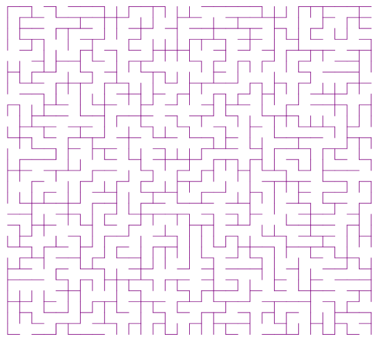
Because of its relationship to random walk, the transfer current appears in the study of many probabilistic models on graphs. The random spanning tree model is the probability measure on spanning trees of which assigns a probability proportional to the products of the edge-weights of the tree (see Figure 1 for a sample).
The transfer current theorem of Burton and Pemantle [7] states that the spanning tree model, viewed as a point process on the set of undirected edges of the graph, is determinantal with kernel . This means that all local statistics have a closed-form expression in terms of the transfer current of the local edges: for any finite collection of disjoint undirected edges in the graph, we have
Any local statistics of the spanning tree is thus a local computation provided we know the value of the transfer current (which depends on the graph in its whole). This is the case for periodic infinite graphs as already pointed out above. Note that the matrix defined above is also a kernel of this process (since it is the conjugate of by a diagonal matrix): since it is symmetric, we say that the spanning tree model is a symmetric determinantal process (this implies further properties of the process that we review in Section 5.6).
In many cases, although an explicit form of the transfer current is not easy to obtain, one can show that on a large scale, or equivalently in the scaling limit for macroscopically distant points, the transfer current is close to its continuous counterpart. For graphs which approximate a smooth domain in a nice way (we call these good approximations), the transfer current between two macroscopically distant edges tends (up to a local constant depending on the edge weights) to the derivative of Green’s function along the directions given by the edges. This is our first main result (see Theorem 1). The proof is an adaptation of the classical arguments from a special case of [9]. The goal is to show the universality of the limit on a large class of graphs in any dimension. Our assumptions on the graph are quite strong (thus the proof is simpler), but these are satisfied by many interesting examples.
Three other models are closely related to the spanning tree model: the two-component spanning forest, the spanning unicycle, and the abelian sandpile model of Dhar [11]. There exist natural couplings between them which enable to express the probability of any event for these models as a spanning tree computation (see [22] for the first two models and see [34, 19] for the abelian sandpile; also see [31]). However, local statistics for these models are not necessarily local statistics for the spanning tree and may require the knowledge of the geometry of the spanning tree as a whole. We focus in this paper only on the local statistics that are local statistics for the spanning tree as well. These type of statistics can be computed explicitly and have a well-defined universal limit, expressed in terms of the scaling limit of transfer currents. This is our second main result (Theorems 2 and 3; another application is Theorem 4).
A possible realization of the random process in a finite subregion is called a pattern. Given a collection of countable patterns on disjoint supports, we can define a new point process, or equivalently a random spin field which is the indicator of the occurrence of these patterns. Under sufficiently fast decay of correlations with the distance, pattern fields of determinantal point processes converge to Gaussian white noise (Theorem 5). We use this to study the fields generated by the local events mentioned above in the spanning tree and sandpile models. More precisely, we express local events fields as pattern fields in the spanning tree model and use the determinantal structure of the spanning tree process to show that these fields are Gaussian white noise. This is our third main result (Theorems 6, 7, and 8). For the special case of the zero-height field of the sandpile on , the result was already obtained by Dürre. The study of pattern fields of determinantal point processes originated in the work of Boutillier [6], who studied them in fluid dimer models on the plane. Gaussian fluctuations for symmetric determinantal point fields were first observed by Soshnikov [38] (this corresponds to patterns consisting of a single point present).
Computing probabilities of local events which are not local for the spanning tree is much harder. In the planar case, it has been addressed by Wilson [40] using methods of Kenyon and Wilson [27].
Describing the scaling limits of spanning trees and related models is challenging. In two dimensions, using conformal invariance, the scaling limit is well understood in terms of Schramm–Loewner evolutions [30]. In dimension three, Kozma [28] has shown the existence of the scaling limit of the loop-erased random walk (that is, the branches of the spanning tree by a theorem of Pemantle [36]) and in high dimension, the scaling limit is also known due to the lace expansion [10]. Furthermore, the geometry of the infinite volume limit has been well-studied [4, 3]. However, many natural questions about the geometry of spanning trees on infinite graphs and their scaling limits remain open. The pattern fields we study encode certain information of spanning trees in any dimension, and their scaling limit might tell us something about the scaling limit of spanning trees. Our method is based on the determinantal nature of spanning trees and the study of its kernel, the transfer current. Pattern fields are local quantities, however we give in Section 4.2, for future use, some properties which relate the transfer current to global geometric properties of trees.
The paper is organized as follows. In Section 2, we introduce some concepts from discrete harmonic analysis: weighted graphs, vector field, derivative, Laplacian, harmonic functions, Green’s functions, and transfer current. In Section 3 we define and exhibit good approximations for domains in . We prove Theorem 1 which states that on good approximations, the transfer current convergences (up to a local factor) to the derivative (in both variables along the direction of the edges) of Green’s function. In Section 4 we review some couplings between spanning trees and the other models and relate the probability of events that correspond to local events for the spanning tree, expressed in terms of the transfer current. We derive from this two types of results: on the one hand, the connection between combinatorics of trees and discrete analytic properties of ; on the other hand, we use Theorem 1 to show that certain correlations of the trees and sandpiles have a universal and conformally covariant limit. Finally, we concentrate in Section 5 on pattern fields of certain determinantal point processes and show as an application of what precedes (for this, we only need the order of decay of in the limit , not its precise value) that the pattern fields of a random spanning tree and the minimal-pattern (e.g. zero-height) fields of the abelian sandpile converge to Gaussian white noise in the scaling limit, under good approximation of a domain.
2. Discrete harmonic analysis
Let be a finite connected weighted graph with vertex-set , edge-set , weight function , and a boundary-vertex-set which consists of a (possibly empty) subset of the vertices. We let and call its elements the interior vertices.
Let denote the space of functions over the interior vertices and be the space of -forms, that is antisymmetric functions over the set of directed edges (two directed edges per element of ). We endow with its canonical scalar product coming from its identification with , that is , and endow with the scalar product given by .
In the case where is infinite, we now abuse the notations and and suppose that these actually denote the subspaces of elements with finite norm (the spaces).
We define the map by and the map by . The maps and are dual to one another, in the sense that for any and .
The Laplacian is defined by , and it is easy to check that for any and , we have
where the sum is over neighboring vertices (including boundary vertices). A function is said to be harmonic at a vertex whenever .
The Green function is the inverse of the Laplacian. Two cases may occur: if the boundary is non empty (), is invertible on , hence . In the case when the boundary is empty (), is the inverse of on the space of mean zero functions. The first one is called the Dirichlet Green function (or wired Green function), the second is called the Neumann Green function (or free Green function) 111Our choice of the qualifier “Neumann” for this Green function comes from the fact that we can replace the free boundary conditions by Neumann boundary conditions by artificially adding a boundary to the graph. The Laplacian acts on the extended space of functions which take same values at any boundary vertex and its adjacent interior vertex. This corresponds to a vanishing normal derivative on the boundary. This modification of the Laplacian does not change the local times of the random walk at interior points which is sufficient for our needs. In the limit, this “Neumann” Green function actually converges to the elementary solution for the Neumann problem.. Given a weighted graph we will sometimes consider simultaneously both Green’s functions by looking at the wired or free boundary conditions.
When the space of harmonic forms, is trivial (which is always the case on a finite connected graph: harmonic functions are constant), the space of -forms has an orthogonal decomposition (Hodge) as
Under this assumption (), when the graph is infinite, Theorem 7.3. of [4] implies that free and wired spanning forests measures coincide.
The orthogonal projection of onto is . Any directed edge defines a -form and we often identify the directed edge with this -form. The transfer current is the matrix of in the basis indexed by . For two directed edges and , it therefore satisfies
| (1) | ||||
According to the boundary condition chosen (free or wired), we obtain two different transfer currents.
A vector field on is the choice for each vertex of an outgoing edge . For any vertex and directed edge , we define to be . In particular, is the neighbor of to which the vector points at. We define the derivative of a function with respect to the vector field to be the function . The derivative of a function with respect to a vector field satisfies , an equality which is coherent with the one from calculus.
The -forms are dual to vector fields and naturally act on them. Another way to see the action of is
Under this formulation, the projection can be written as acting on the divergence of vector fields with kernel given by Green’s function. The continuum analog of this projection is widely used and is known as the Hodge-Helmholtz projection.
3. Scaling limits
3.1. Good approximations of domains
Let and be a simply connected open set, with smooth boundary . We call such a set a domain. We consider a sequence of connected weighted graphs with boundary-set embedded in . By “embedded”, we mean that the vertices are points inside and boundary vertices lie in . The edges are mapped to smooth non-intersecting segments in such a way that edges between boundary vertices lie inside . We let be the Laplacian on .
We say that a sequence of functions , converges uniformly on a compact subset of to a function , if the sequence defined by converges uniformly to on .
We say that the sequence is a good approximation of if the following properties hold.
-
(1)
(Approximate mean value property) For any bounded harmonic function on , and any ball , we have .
-
(2)
(Paths approximation) For any straight line in joining to , there exists finite paths inside joining two vertices to such that , , and uniformly tends to a path . Moreover, the discrete length of is bounded by an absolute constant times the length of .
Examples of good approximations include: the lattices for and for some domain (the Approximate mean value property follows from Lemma 6 in [20]; the Paths approximation property is clear), and for , isoradial graphs with bounded half-angles, see [25] (see Appendix A for a quick review of the definition of isoradial graphs and a justification of why there are good approximations).
The Paths approximation property is rather easy to check on a given graph. It is less so for the Approximate mean value property: see Remark 4 below for a practical way to check it.
3.2. Convergence of the derivative
In the following, denotes the Euclidean length of the edge viewed as an embedded segment. For any vertex , we denote the discrete ball of center and radius in , and by its cardinality.
We say that a compact subset of is interior if its distance to the complement of is strictly positive.
Proposition 1.
Let be a good approximation of a domain . Consider a vector field . Suppose a sequence of harmonic functions on converges uniformly on interior compact subsets of to a harmonic function . Then the sequence of their rescaled discrete derivatives is uniformly close in the limit , on all interior compact subsets of , to the derivative of .
Proof.
Let be a compact subset of . Let be an interior compact subset such that and is at a positive distance from the exterior of . The function is bounded on , hence the sequence as well. Let and be an approximation of . By the approximate mean value property at and , there exists a constant such that, for any , we have
Now,
where we used, in the last equality, the bound of on the surface-area-to-volume ratio of a ball or radius in . The sequence is therefore uniformly bounded on .
Therefore, one can extract a subsequence , so that converges uniformly on compact subsets to some bounded function . We now prove that for any subsequential limit , which finishes the proof.
By the Paths approximation property (and because is locally convex), for any close enough, and any , we can take a discrete poly-line segment , such that , , and converges (in the uniform topology) to the line . We replace the vector field along this line so that it is aligned with it. Along a subsequence , we have
Taking , uniform convergence implies
By taking at every , and letting , we have . ∎
Remark 1.
Since the derivative of a harmonic function is a harmonic function, Proposition 1 may be applied successively to show that any higher order derivative also converges under the same assumptions.
3.3. Green’s function and transfer current
In this paper, we consider to be the positive definite Laplacian. Recall that the Green function with Neumann (resp. Dirichlet) boundary conditions is the (unique up to constant) smooth symmetric kernel over solution to
with boundary condition for , where is the normal vector at the boundary point (resp. for ). On a bounded domain the Neumann Green function is defined up to an additive constant, and we identify it with its action on functions of mean zero.
We now make some further assumptions on our good approximations. First, we suppose that they form an exhausting sequence of some infinite embedded graph . We assume that Green’s function on , denoted by , converges uniformly, upon rescaling, on compact sets (away from the diagonal) to the continuous Green’s function on with control on the error term, and that the invariance principle holds:
-
A1
(Green’s function asymptotics) .
-
A2
(Invariance principle) The random walk on converges in the supremum norm to Brownian motion in .
These assumptions are satisfied by the following good approximations: the lattices , see [15, 29], and for , isoradial graphs, see [25, 9] and Appendix A.
Theorem 1.
Suppose the conditions of Proposition 1 hold. Then under assumptions (A1) and (A2), we have
| (2) |
where is Green’s function with the corresponding boundary conditions on , and its differential.
Proof.
Let denote the transfer current associated with Green’s function on the whole space, defined in (1). By Assumption A1, the rescaled Green’s function on the infinite graph converges uniformly on all interior compact subsets to Green’s function on the whole plane . Applying Assumption A1 to (1) and differentiating twice, we have
| (3) |
Consider the discrete harmonic function . By the invariance principle (Assumption A2), converges to the continuous harmonic function with boundary values given by . Applying the same (mean value) argument as in the proof of Proposition 1, the discrete gradient of is uniformly bounded. Therefore converges to , uniformly on interior compact subsets of . By applying Proposition 1 twice, we obtain the uniform convergence of the rescaled double increment of to the double derivative of . Since
combined with (3), this implies
which finishes the proof. ∎
Remark 2.
Remark 3.
By using the interpretation of Green’s function as the density of time spent in the neighborhood of when started at and the explicit Brownian time-space scaling, one can use (A2) to prove a weaker form of (A1), namely that .
Remark 4.
If we suppose that the discrete Laplacian of homogeneous polynomials of degree in is , where is the coefficient of , then, by using (A.1), the Approximate mean value property may be shown, following the proof of Proposition A.2 in [9]. This assumption also implies that random walk is isotropic (and the variance of the increments is of order of the volume around each vertex) and thus implies (A.2).
As in the setup of [24, Theorem 13], in order to control the behavior of Green’s function for points on the boundary, we slightly modify the way we approximate the domain by ensuring that the approximating graphs have piecewise linear boundaries in the following sense. We consider a sequence such that , as , and an increasing sequence of domains such that lies within of and such that its boundary is a polytope (polygon, when ) with hyperfaces (segments, when ) of size . is furthermore assumed to be convex for .
We can obtain convergence of the transfer current for points on the boundary whenever we consider, as a replacement of a good approximation to , a diagonal subsequence of good approximations of the domains . This follows from the fact that on domains with piecewise linear boundaries, we can use a reflection argument.
Corollary 1.
Let , be a convex domain with smooth boundary, or be simply connected with smooth boundary. Assume the approximation sequence is chosen as above. Formula (2) holds for points on the boundary.
Proof.
Reflect the approximation graph of across the flat piece of the boundary, and glue it with the original graph. The result follows by noting that Green’s function on the new graph is a linear combination of Green’s function on the original graph. When the argument works for any simply connected surface (see Proposition 7). ∎
3.4. Planar graphs
On any planar embedded graph, the conjugate of a harmonic function on the graph is a harmonic function on the planar dual which is defined by the following discrete Cauchy–Riemann equations: (for any directed edge , denote by the dual edge directed in such a way that ) for any dual edges and (where is the discrete derivative in the dual and primal graph, respectively).
In particular, we have the following.
Lemma 1.
Let be the Green function of a planar graph . Let be the harmonic conjugate of . For any , let be the dual edge to . We have
where is the Green function on the dual graph .
Lemma 1 is the discrete analog to the fact that the ‘complex’ Green function defined as where is the Dirichlet Green function and the Neumann Green function, is analytic (away from the diagonal) hence satisfies the Cauchy–Riemann equations.
On the whole plane, we can compute this explicitly for comparison. Start with . Then by taking the harmonic conjugate (in one of the variables) we obtain (it is the same in either variable by a simple geometrical fact about parallel angles being equal). Now taking the harmonic conjugate with respect to the other variable we get back again, up to an additive constant. By taking differences of Green functions as in the lemma we get equality.
Proof of Lemma 1.
Let . The function is harmonic with a defect of harmonicity at and at . Its harmonic conjugate is the function . This is a univalued harmonic function with a defect of harmonicity at and at (This may be seen by comparing the harmonic extension of avoiding edge and the harmonic extension crossing that edge. Since this move is local, when one extends from to , one obtains the result). Thus it is equal to . ∎
Corollary 2.
Let and be two edges. Then
where is the transfer current on , and the transfer current on the dual graph .
4. Transfer current in statistical physics
In this section, we explain ways in which the transfer current describes models of statistical physics on weighted graphs: point correlations and geometrical properties. Using Theorem 1, we can find the scaling limits of some of these expressions. We also relate analytical properties of to its combinatorial properties.
4.1. Spanning trees
Let be a finite connected weighted graph. A spanning tree on is a subgraph , where is a set of edges, which contains no cycles and is connected. We weight each spanning tree by the product over edges in the tree of their weight and call the corresponding probability measure the random spanning tree on .
By the transfer current theorem of Burton and Pemantle [7], the transfer current is a kernel for the random spanning tree measure, that is, for any distinct edges , the probability that the random spanning tree contains them is
Given an edge in , we let denote the random variable that takes value if belongs to the spanning tree, and otherwise (this is an example of a pattern field, defined in Section 5 below). For distinct edges , the covariance of the corresponding random variables is .
Theorem 2.
Under the assumptions of Theorem 1, the rescaled correlations of the spanning tree model have a universal and conformally covariant limit.
4.2. Two-component spanning forests and spanning unicycles
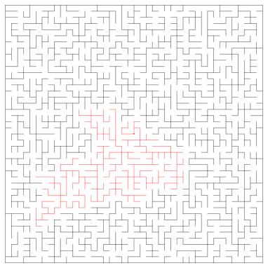
A two-component spanning forest (SF) on is a subgraph , where is a set of edges, which contains no cycles and has exactly two connected components. A spanning unicycle (or cycle-rooted spanning tree) is a connected subgraph where (it thus contains a unique cycle). See a picture on Figure 2. On planar graphs these two notions are dual to one another. In the following we do not need to suppose however (unless otherwise stated) that the graphs are planar.
As for spanning trees, we consider the weight of a subgraph to be the product over edges (of the subgraph) of the edge-weights. We define a probability measure on SFs (respectively, random spanning unicycles) by giving a SF (respectively, a spanning unicycle) a probability proportional to its weight. This defines the random SFs and random spanning unicycles considered hereupon.
A spanning unicycle can be thought of as a spanning tree to which an edge is added. Note however, that the measure obtained from taking a random spanning tree and adding a uniformly random edge is different than the random spanning unicycle defined above, and the Radon-Nikodym derivative is simply the length of the cycle. Nevertheless, we observe that the law of the cycle of the random spanning unicycle conditional on the event that the cycle contains some edge is the law of the path between the extremities of in the spanning tree model on the graph where is removed. The event that the cycle is of a given shape is therefore the union of translates of events for the spanning tree, which can be evaluated explicitly for infinite periodic graphs. In particular for , using the explicit values of the transfer current computed in [7], we obtain that the probability that the cycle is of length is .
 |
 |
Let be the weighted sum of spanning trees and the weighted sum of spanning unicycles. In the following, whenever denotes a directed edge , we say that is its head, and its tail. Furthermore, the symbol denotes the directed edge with same support and opposite direction, that is, .
In the wired case (), using the fact (Theorem 3 of [22]) that is the weighted number of two-component spanning forests such that and are disconnected from the boundary, we have for any two directed edges and ,
| (4) |
where is the weighted number of two-component forests such that the extremities of belong to different components, as well as for the extremities of , and these are the same for both heads and both tails.
In the free boundary case (), we start with the following result.
Lemma 2 (Lemma 1.2.12 in [21]).
Let be the set of all spanning unicycles. For any , we have
where and is the choice of a directed representative of the unique cycle of the unicycle .
Proof.
It is an immediate corollary of Proposition 7.3 of [5]. The map is the orthogonal projection on , which is the orthogonal complement of . Recall from [5] that a fundamental cycle associated to a spanning tree and a directed edge not on the tree, is the directed cycle defined by the union of that edge with the unique path joining the extremities of that edge in the tree (the direction of the cycle is given by the direction of the edge). A basis of is given by the (-forms corresponding to) fundamental cycles associated to a spanning tree. Hence
where is the fundamental cycle of in . ∎
Remark 5.
Lemma 2 may also be proved by expanding the determinant of the line bundle Laplacian (introduced in [26]) around the trivial connection along (that is, expand near the family of Laplacian determinants associated to the connection ). This yields yet another geometric interpretation of the transfer current.
In the planar case, we obtain the following. Taking to be the indicator on directed edge on the dual graph, we have
| (5) |
where is the number of spanning unicycles, the cycle of which contains and . In the planar case, the dual of a SF is a spanning unicycle. It follows from (4) and (5) that , which gives another proof of Corollary 2 above.
Lemma 2 gives a way to compute the expected winding of the cycle of the spanning unicycle.
We conclude this subsection by giving two applications of Theorem 2 to the case of planar graphs or graphs embedded in .
For planar graphs with two marked faces and ’, let and be the set of east-directed edges crossed by two disjoint dual paths from the outer face to and ’, respectively. Taking to be the -form indicator of and , we obtain that the probability that two faces lies inside the cycle of the uniform spanning unicycle on a planar graph is
This formula simplifies to by Corollary 2 and was observed in [22]. For any isoradial graphs, the ratio converges to a constant , see [23] (and [31] for the case of ).
In the case of , we obtain the following.
Corollary 3.
Consider to be the subgraph of whose vertex-set is . Let be a face in the plane with coordinates . Let be the winding number of the uniform spanning unicycle in around the tube . Its second moment is given by
where , and is a constant.
Proof.
Consider a -form defined to be the indicator of the edges on a directed “curtain” of edges that connect the tube to the boundary of : more precisely we consider a path in the plane from to the boundary and the curtain consists of the edges on oriented consistently. In that way, any oriented simple closed curve satisfies where is the algebraic winding number of that curve around the tube.
4.3. Minimal subconfigurations of the abelian sandpile
The abelian sandpile model is constructed as the stationary distribution of a certain Markov chain on integer functions over interior vertices of a graph. A sandpile configuration is a particle configuration . If for some we have , then the vertex may topple, that is send one particle to each of its neighbors (this corresponds to the operation ). Particles that reach the boundary (referred to as the sink in this context) are lost. A sandpile is stable if for any . A bilinear operation can be defined on the set of stable configurations: addition in followed by toppling until stabilization. (The order in which toppling occurs does not matter, it is an abelian network [11].)
The Markov chain on the set of stable sandpiles is the following. At any given time, add (using ) a particle to the configuration at a uniformly chosen vertex in . It was shown in [11] that the stationary distribution of this chain is unique and is uniform on the set of recurrent states. The recurrent configurations of the sandpile are defined as the recurrent states of this Markov chain.
The set of recurrent configurations has a local description given by the burning algorithm [11]. A stable configuration is recurrent if and only if any subconfiguration satisfies that it is unstable regarded as a configuration on the subgraph on which it lives. Using this criterion, Majumdar and Dhar constructed a bijection (called the burning bijection) mapping recurrent configurations of the abelian sandpile to spanning trees [34, 35]. It depends on the choice of an ordering of edges around each vertex. See [37] for a theoretical physics perspective on the sandpile as a field theory.
In the case of a weighted graph, we define a measure on the set of recurrent configurations which is the pullback of the weighted spanning tree measure under the burning bijection. There is a way to relate to the discrete projection of the continuous sandpile (whose dynamics is analog to the one described above for unweighted graphs [16, 23]).
Under the burning bijection, any local event for the sandpile therefore translates into an event for the spanning tree, however not necessarily local. An important concept is that of minimal subconfiguration (the original definition is from [12] where it is called weakly allowed subconfiguration).
A subconfiguration on a subgraph is minimal if it is part of a recurrent configuration, but by decreasing any of its heights, this is no longer true. In particular, conditional on a minimal subconfiguration, the measure on the outside of is the sandpile measure on , still with sink at .
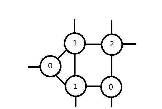
The easiest example of a minimal subconfiguration is a single vertex with height , or any collection of vertices with height provided none of these vertices are neighbors. There are minimal subconfigurations on any subgraph of , see Figure 3 for a more elaborate example.
Let be the graph obtained by wiring all the vertices in with , and removing all self edges. The following proposition is the generalization of Theorem 1 of [19] to the weighted graph setting.
Proposition 2.
Given any spanning tree of , let be the edge set
For any minimal configuration supported on , there is a spanning tree of (given by our choice of burning bijection) such that
where the sums are over spanning trees of .
Proof.
By Lemma 4 in [19], the minimal subconfigurations are mapped (by the burning bijection) to spanning trees for which the projection of the tree on is again a tree. Therefore, the probability of a minimal configuration is the probability that the small tree is the image of the subconfiguration on . By the Gibbs property of the weighted spanning tree measure, this is simply the probability that the tree measure on does not contain the edges of . Under the choice of orientation, the probability that (for a fixed subconfiguration) we map it to is proportional to the edge weights in the tree. ∎
Theorem 3.
Under the hypotheses of Theorem 1, the rescaled correlations of a finite number of macroscopically distant minimal subconfigurations has a universal scaling limit. In particular, the rescaled correlations of zero heights converge to a universal scaling limit (which is conformally covariant in dimension ).
4.4. Discrete Gaussian free field current flow
The discrete Gaussian free field (DGFF) (with free or wired boundary conditions) is the Gaussian vector with zero mean and covariance matrix given by Green’s function (with free or wired boundary conditions).
The current flow of the DGFF, defined by , is a Gaussian -form with zero mean and covariance matrix given by the transfer current, since for any -form , we have
where we used the fact that and are dual.
Whenever the discrete Green function converges to the continuous one, the discrete Gaussian free field converges weakly in distribution to the continuous Gaussian free field. In virtue of Theorem 1, it is also the case for the current flow, which converges to its continuous counterpart.
Theorem 4.
Under the hypotheses of Theorem 1, the flows converge weakly in distribution to , where is the GFF and the derivative is in the distributional sense.
5. Random point fields
5.1. Patterns
A simple point process (point process for short) on a discrete 222The result of this section easily adapts to the case of (uncountable) Polish spaces but we restrict to the discrete case to avoid cumbersome technicalities. space is a random subset , or equivalently, a random configuration of -valued spins at each point . We define a pattern to be a finite (deterministic) spin configuration which can be represented as a pair of disjoint sets , where is the set of points with spin and the set of points with spin . The support of a pattern is the set which we denote by . We say that two patterns are disjoint when their supports are disjoint. A mono-pattern is a pattern where all spins have the same value.
Given a collection of patterns , a point process on induces a point process on the disjoint union of the patterns, which we may still view as a point process on (for example, by fixing an ordering of points in and identifying the pattern with its element of least index). This is the pattern field associated to .
Formally, a pattern field can be represented as , which is an element of the dual of . We will omit the dependence on if it is clear from the context. For any , we write and if is the indicator of a subset .
5.2. Symmetric and block determinantal processes
Let be the kernel of a trace-class self-dual map in with eigenvalues in , that is a symmetric matrix indexed by . For any finite set , denote the restriction of onto . Let be the diagonal matrix with s on the entries indexed by and elsewhere. defines a symmetric determinantal process, which means that for any pattern , we have
| (6) |
The kernel is a kernel for the complement process .
Although the underlying point process is determinantal, the pattern field is not. However, joint probabilities of patterns can still be written as a large minor of a modified matrix. More precisely,
| (7) |
Therefore it can be viewed as a block determinantal process, see Section 5.3 for more details.
It follows from a short computation that for any finite set , we have
| (8) |
which signifies that the number of points in is a sum of independent Bernoullis. These facts are well-known, see e.g. Chapter 4 of [17] for an introduction to determinantal processes.
Proposition 3.
Let be a symmetric determinantal point field. Let be a family of disjoint patterns. The number of points observed in , where is any finite subset, is a sum of independent Bernoullis.
Proof.
For any finite set of patterns , we have
In the case when the patterns are singletons, is just a subset of , and
Thus the variance is given by
5.3. Fluctuations for block determinantal processes
Before studying the scaling limits of pattern fields, we show (following ideas of Boutillier [6]) a fluctuation result for general block determinantal fields (without assuming the kernels to be symmetric). In combination with the covariance structure studied in the next section, this implies that under the right decay of correlation, pattern fields of determinantal processes converge to Gaussian white noise.
Let and be a domain. Let be the space of locally finite particle configurations in . Denote to be the measurable subsets of , generated by the cylinder sets
where is a Borel set and . is said to be a block determinantal process, if for any and ,
where the point correlation function
| (9) |
and each is a matrix. We will abuse the notation below and let denote .
Proposition 4.
Let be a family of block determinantal processes. Assume that is bounded from below by a strictly positive constant, and converges as to a limit satisfying as . Then a rescaling-recentering of the associated point field converges weakly in distribution to a Gaussian field: for any test function , we have
We will prove the proposition by verifying Wick’s theorem for the counting field, and shows the finite dimensional distributions converge to that of a Gaussian field (see e.g. [18]). The Wick’s theorem states if is a random field such that all of its moments can be expressed in terms of the covariance structure as follows: for any smooth test functions ,
| (10) |
then is Gaussian. In practice, by polarization identities it suffices to check the above identity for .
The basic idea is that when computing higher moments, all the contributions not coming from pair correlations vanish, since the correlations decay fast enough. The argument follows the spirit of [6].
Proof.
We first verify the Wick formula in the case where the contribution points are macroscopically distant. Let
Note the following exclusion-inclusion formula
where .
Now expand the determinant, and notice that the off-diagonal entries of the matrix are small (bounded by ). One can rewrite the above expression in terms of sums over permutations fixing no block (or equivalently, as products of cycles), and the support of which intersect each block exactly once. We thus obtain
where the term accounts for the contribution from permutations that has at least two non-fixed point in some block. Indeed, for a particular that partitions into cycles , one can write
Let denote some partition of . Therefore,
It suffices to show all the contributions from a cycle of length vanish. It is easy to verify that
Therefore each term arising from a cycle of length is bounded by
| (11) |
for some . Since , the decay rate of is the same as , which implies that for any . Apply the following elementary inequality to (11),
and note that each term can be bounded by . For instance, the first corresponding term satisfies
by successively summing over . Therefore (11) can be bounded by , which vanishes in the limit for .
All the terms contributing to the limit are thus coming from pairings, and we verified Wick’s formula (10).
When the ’s are not necessarily all distinct, we can verify the Wick formula for higher moments by the same argument as in Section 3.2.2 in [6], and we omit the computation here. ∎
5.4. Central limit theorem for pattern fields
Suppose that is infinite and embedded in in a discrete way (no accumulation points). Let be a simply connected domain containing . Define : these sets (when remultiplied by ) form an exhausting sequence of subsets of . We suppose that each is equipped with a determinantal process with kernel . We assume that pointwise. This implies that the point process on is the weak limit of the process defined on . As we will see, this implies that scaling limits of fields constructed from local events do not feel the influence of the boundary shape of .
For each , let be a collection of patterns in . When the choice of is fixed, we write instead of .
Theorem 5.
Assume that . If for any and , is uniformly bounded from below, then as , converges in law to a standard Gaussian.
In the case where the patterns are singletons, the only condition we require is that , and the result follows from the Lindenberg–Feller theorem as explained in Theorem 4.6.1 of [17].
Proof.
By pointwise convergence of to , we have for any . The result now follows from Proposition 4 since the pattern field is block determinantal. ∎
It follows from Theorem 5 that the rescaled-recentered field constructed from converges to a Gaussian field, that can be viewed as a random element of . By the lower bound on , the growth rate of is (which we will take to be of the order of ) and compute the covariance structure of the Gaussian random field obtained as the limit of .
To characterize the law of a Gaussian field, it suffices to compute for any test function (see [18]). If
then is a Gaussian field with correlation kernel . When , where is the Dirac mass and , the field is Gaussian white noise, is proportional to and is called the intensity.
Let be an increasing sequence of finite collections of disjoint patterns on , such that . Denote . We consider the associated random fields .
Assume to be periodic (as an embedded set), that is, suppose it has a finite number of orbits under the action of a rank group of translations . We also suppose the collection of patterns itself to be invariant under , that is, it can be written as the disjoint union of the translates of a finite collection of patterns .
Theorem 6.
Let be a periodic subset of as above. Let be a simply connected domain containing and define . We suppose that on each of these is defined a determinantal process with kernel satisfying the conditions in Theorem 5. Then, for any periodic set of patterns generated by a pattern , the corresponding field satisfies that converges weakly to a Gaussian white noise with intensity
| (12) |
Proof.
As explained above, we already know that the limit exists and is Gaussian. Let us identify the covariance structure. In the following, we make the abuse of notation to denote the value of where is the location (center of mass) of the support of the pattern.
Given any test function , we have
| (13) |
Consider a small (and write for ). We split the previous sum into three contributions as follows
We will show that the main contribution comes from the third term.
By the assumptions of Theorem 5, we know that there is a matrix such that for , we have
which is a finite alternating sum of products that contain at least two off-diagonal block terms. Every such term is bounded by
where . Therefore .
The first term therefore yields a contribution of . Due to the smoothness of , the second term yields a contribution of
since the sum of covariances is absolutely convergent.
The third term yields a contribution of
which, by periodicity, converges, as long as , to
| (14) |
where .
In the case of singleton patterns, the intensity can be written as
5.5. Interpretation of the intensity
Suppose the determinantal point field is at the same time a Gibbs random field, in the sense that the weight of any configuration is given by , for some . In that case, the noise intensity can be interpreted as a second derivative of a free energy. Indeed, the partition function is defined by . In particular, for a fixed pattern , choose the weight function so that it gives weight on , and on all . Let be the corresponding partition function. A short computation shows that , which can be interpreted as an electric susceptibility of the network.
5.6. Pattern fields of the spanning tree model
Let , be a bounded simply connected domain containing . Let be an infinite weighted graph embedded in invariant under a rank lattice . We define to be the edge-set of .
The spanning tree model on is a symmetric determinantal process on with kernel given by the transfer current (another kernel, which is symmetric itself, is the matrix defined on page 1 in the introduction).
In this context, a pattern is a finite set of edges in a fundamental domain of , where the edges are present and are forbidden. Suppose that lies inside a fundamental domain , and let denote the union of its translates that lie inside . We define the corresponding pattern field , where denotes the translate of pattern by .
The mean of the pattern field on a finite set may sometimes be computed: when and is isoradially embedded, the density of edges has the following limit. The probability of an edge on an isoradial graph is , where is the half-angle of that edge by [25] (see Appendix A). Hence, the expected number of edges in a finite set is
Theorem 7.
Under the assumptions of Theorem 1, each rescaled pattern density field converges weakly in distribution to Gaussian white noise. The sum of two pattern fields also converges to Gaussian white noise.
Proof.
The intensity of the white noise is given by (12). When we study correlation among fields (that is, the cross-term in the covariance structure of the sum of two pattern fields), say between two fields corresponding to patterns and , which generate two collections and , the intensity (which may be negative) is given (computation omitted) by
Let us give the example of an infinite -regular graph: at each vertex, edges are numbered . We consider the pattern field generated by all edges of type . The intensities of the joint fields are denoted . Since the total number of points in is constant ( is a projector), for any , we have . Hence, we obtain
| (15) |
A similar relation is true for the liquid dimers pattern fields in two dimension, see the remark following Theorem 7 in [6].
When is the collection of all edges, and , the non-rescaled covariance of the variables (which represents the number of edges inside ) has a limit. (A similar statement is true for other patterns.)
Proposition 5.
Under the assumptions of Theorem 1 and given two disjoint subregions and of , the correlation between the number of edges and is
Proof.
This follows from Theorem 1. ∎
5.7. Minimal-pattern fields of the abelian sandpile
Minimal subconfigurations of the sandpile correspond to local events for the spanning tree model. However, they cannot always be written as simple patterns: the probability that a vertex has height zero is equal to a weighted sum of the probability of (non-disjoint) patterns consisting of a single edge present (and all other missing). We therefore need to deal with the mixture of measures and an argument is provided in the following proposition.
Proposition 6.
Let be a random element in that satisfies a central limit theorem (as a sequence in ), be a random measure on finite subsets of . For any , , where are uniformly bounded, and the sum runs over all the elements of . Then satisfies a central limit theorem with the same speed.
Proof.
The result follows by directly verifying Wick’s formula. Consider the moment of the rescaled field applied to a test function :
It suffices to check
This is easily verified using the corresponding result for . For instance, when is even, only contains contributions from the sum of point marginal () of Each of these marginals can be expressed as a finite linear combination of point marginals of . The central limit theorem for implies that the corresponding sum of point marginals of is . Therefore . ∎
We now study the abelian sandpile model on the following class of graphs. Let be an infinite weighted graph embedded in , and invariant under a rank lattice . This graph is in particular amenable and satisfies the one-end property [33]. The infinite volume limit on sandpiles is thus well-defined [1, 19].
Let be a domain. Without loss of generality, we may suppose that lies inside the domain and we define . For a fixed minimal subconfiguration (that we call minimal-pattern) lying inside the fundamental domain , let be the collection of its translates lying inside . Let be the associated random field in .
Theorem 8.
Under the assumptions of Theorem 1, and for any minimal-pattern, the corresponding field converges weakly in distribution to Gaussian white noise.
Proof.
When is a regular lattice with uniform weights, each spanning tree described in Proposition 2 carries the same weight. Therefore we can choose a pattern for the spanning tree model (on the edges of the graph) such that the minimal-pattern is in bijection with the event under the burning bijection. The field can therefore be seen as a pattern field of the spanning tree model (associated to ) (note that the union of two adjacent minimal subconfigurations occurs with zero probability, because of Dhar’s burning test). The result is then a corollary of Theorem 7.
Let us deal with the general case. We start by showing that the limit exists and is Gaussian. Recall from Proposition 2 that the probability of a minimal subconfiguration is a linear combination of pattern probabilities for the spanning tree model. By Proposition 6, it suffices to prove the result for a fixed tree pattern . This follows from Theorem 7.
The intensity of the field is computed as follows. The probability of having two adjacent minimal subconfigurations is zero. The intensity of the white noise which is of the form (12) does not include adjacent patterns. Therefore, each covariance can be replaced (using Proposition 2) by a linear combination of expressions involving the transfer current. It may therefore be evaluated using the explicit formula for the transfer current when this latter is known.
In the special case of the zero height field, one has , where is the height of sand at . The asymptotic density of zero height is known in certain cases. Let be some set of vertices. We have , where and . In the case of , the fundamental domain has size and by using the explicit expression of the transfer current (see [34] for the computation).
6. Questions
-
(1)
We have not dealt with non-minimal subconfigurations in the sandpile: do the corresponding fields also have Gaussian fluctuations?
-
(2)
Can closed-form numerical expressions be obtained for the different intensities of the pattern fields? Are there algebraic relations between different intensities, generalizing (15)?
-
(3)
From the proofs above, one sees that the critical rate of correlation decay in dimension is , where is the distance. If the correlation decays faster, the random field fluctuations converge to Gaussian white noise. Boutillier [6] studied the random field associated with liquid dimers on planar graphs, which are in the critical regime, and obtained some long range Gaussian random field in the limit. Are there any natural critical models in higher dimensions?
-
(4)
Does the approximate mean value property hold for supercritical percolation cluster and random conductance models, thus allowing one to study the scaling limit of statistical physics models on these random environments? In the random conductance model on [2] the Green function is shown to have the same decay as the continuous Green function. Provided the approximate mean value property is valid, one can show that the transfer current has the decay of which implies that the pattern fields considered above (on this random environment) would have the same fluctuations as in the current paper.
-
(5)
What is the distribution of the number of points of a pattern field for a symmetric determinantal process on a finite space?
Appendix A Isoradial graphs
In this appendix, we recall why isoradial graphs are good approximations of planar domains which satisfy Assumption (A1) and (A2) (on page A1) about the convergence of the Green functions on the whole plane. Our main reference for this section is [9].
Good approximations
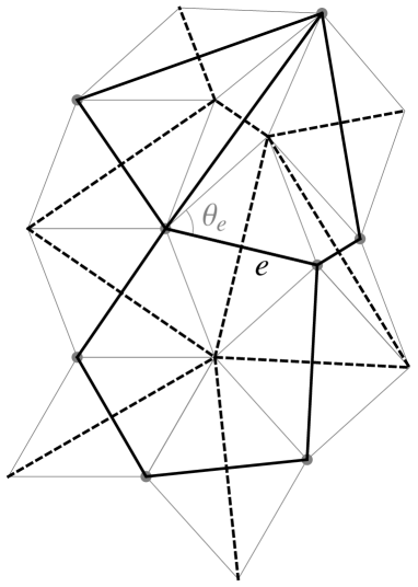
Let us first recall the setting (see e.g. [25, 9] and references therein for earlier works on the subject). Let be an infinite planar isoradial graph and for each we denote by a planar isoradial embedding of with mesh size (we may suppose that an isoradial embedding of with mesh size is fixed and that other embeddings are obtained by dilation with respect to a fixed vertex). The planar dual of is also isoradial with same radius and the diamond graph is defined to be the graph whose faces are the rhombi for all edges , obtained by joining the vertices of an edge and its dual. The angle between an edge and the side of at its left is denoted . It is the half-angle at the origin of edge of the rhombus , see Figure 4.
We make the customary assumption (bounded half-angles property) that all angles of these rhombi are uniformly bounded away from and . This ensures that for vertices of , the combinatorial distance in the graph and the Euclidean distance are uniformly related by a factor of . Let be a simply-connected compact planar domain. For every , consider to be a finite isoradial subgraph of whose vertices lie in , which is “simply connected” in the sense that the union of its closed faces is simply connected. A sequence is said to approximate if the Hausdorff distance from to is .
In the following, we assume that is endowed with its critical isoradial conductances
where is the half-angle of the rhombi (see [25] for a longer definition), and consider the corresponding Laplacian .
It is shown in [9] that isoradial graphs satisfy the Approximate mean value property. The Paths approximation property follows from the bounded angle property mentioned above. Thus, isoradial graphs are good approximations.
Furthemore, the random walk (biased by weights) on the embedded graph is isotropic. A local time-reparametrization of it converges to Brownian motion. This implies assumption (A2).
Green’s functions convergence
It was proved by Kenyon in [25], up to an improvement given by Bücking in [8], that the Green function on satisfies the following expansion 333On , an all-order expansion is known [15].: for any two vertices , we have
This implies that converges to the Green function on the whole plane , as .
This is assumption (A1). We have thus recalled why isoradial graphs are good approximations satisfying assumptions (A1) and (A2).
Since the Laplace equation is conformally invariant, for any simply-connected surface with boundary, , the Neumann and Dirichlet Green function are obtained by their image under a conformal map between the upper half plane and of the Green function on with corresponding boundary conditions.
Discrete harmonic functions on isoradial graphs converge to continuous harmonic functions in a very strong sense described in [9]. In particular, the Dirichlet Green function is shown to converge building on Kenyon’s asymptotics for the whole plane. We give here the proof for the free boundary Green function. The proof follows from arguments in [9] although the result is not stated explictly there.
Proposition 7.
For any graph approximating a simply connected surface with boundary in the sense that is embedded in and there exists a system of coordinate patches and conformal maps that map the graph to an isoradial planar graph on these patches, the discrete Neumann Green function converges uniformly on any compact set inside the surface to its continuous counterpart.
Proof.
Let us first show it for the unit disk . Let be an infinite isoradial graph with mesh size such that is a subgraph of it. Write where is harmonic with Neumann boundary conditions equal to the normal derivative of . By convergence of when the mesh size goes to zero, the values of the normal derivative converge. Now consider the dual graph of . The harmonic conjugate of is univalued since is simply-connected. Its values on the boundary are determined (up to a constant which we take to be ) and converge to a limit . By [9] the harmonic function converges to the harmonic extension of . Hence, its dual converges too, to a function . The limit of is therefore which is equal to Neumann Green’s function (up to a constant).
In the case where is another domain (even non planar), we use a conformal map to bring it back to the previous case. Since convergence is a local result, we may again use the convergence result of [9] and the above argument. ∎
Comments on previous related work
Asymptotics of the Green function on isoradial graphs and its derivatives have been well studied in the literature. Among others, we may state [39, 15] for asymptotics of the Green function on and [25, 8] for the case of isoradial graphs on the whole plane (stated above). For the convergence of the increment rate of the rescaled Green function over , see Lemma 17 in [24].
Dürre in [14] showed in the case of in the Dirichlet case the analog of our Theorem 1 and also gave the application to the study of zero-height fields in the abelian sandpile (our Theorems 3 and 8 for this particular minimal-pattern in the case of ).
Important results of convergence of discrete harmonic functions and their derivatives (in the Carathéodory topology) in domains with boundary (in particular the Dirichlet Green function) to their continuous counterpart are gathered in [9]. Theorem 1 directly follows from their arguments in the case of isoradial graphs by using convergence of the wired Green function in each variable. For the free case it follows from Proposition 7 above.
Carathéodory convergence is weaker than Hausdorff convergence, which we suppose. Therefore, the results of [9] applied to the transfer current give the uniform convergence.
Note that for isoradial graphs there is an explicit formula for the transfer current in terms of path integral which is a linear combination of the Green function explicit formula derived in [25]. We do not use it here because we are interested only in the scaling limit asymptotics which are easier to derive.
Acknowledgements
We thank Cédric Boutillier, Richard Kenyon, and David Wilson for helpful discussions and feedback. We also thank the anonymous referee for helpful suggestions.
References
- [1] S. R. Athreya, A. A. Járai, Infinite volume limit for the stationary distribution of abelian sandpile models, Communications in Mathematical Physics, 249 (2004), 197–213. MR2077255 (2005m:82106)
- [2] M. T. Barlow, J.-D. Deuschel, Invariance principle for the random conductance model with unbounded conductances, Ann. Probab. 38 (2010), no. 1, 234–276. MR2599199 (2011c:60329)
- [3] I. Benjamini, H. Kesten, Y. Peres, O. Schramm, Geometry of the uniform spanning forest: transitions in dimensions 4,8,12,…, Ann. of Math. (2) 160 (2004), no. 2, 465–491. MR2123930 (2005k:60026)
- [4] I. Benjamini, R. Lyons, Y. Peres, O. Schramm, Uniform spanning forests, Ann. Prob. 29 (2001), 1–65. MR1825141 (2003a:60015)
- [5] N. Biggs, Algebraic potential theory on graphs, Bull. London Math. Soc. 29 (1997), no. 6, 641–682. MR1468054 (98m:05120)
- [6] C. Boutillier, Pattern densities in non-frozen dimer models, Comm. Math. Phys. 271 (1) (2007), 55–91. arXiv:math/0603324
- [7] R. Burton, R. Pemantle, Local characteristics, entropy, and limit theorems for spanning trees and domino tilings via transfer impedances, Ann. Probab. 21 (3) (1993), 1329–1371. MR1235419 (94m:60019)
- [8] U. Bücking, Approximation of conformal mappings by circle patterns, Geom. Dedicata 137 (2008), 163–197. MR2449151 (2010k:30054)
- [9] D. Chelkak, S. Smirnov, Discrete complex analysis on isoradial graphs, Adv. in Math. 228 (3) (2011), 1590–1630. MR2824564 (2012k:60137)
- [10] E, Derbez, G. Slade, The scaling limit of lattice trees in high dimensions, Comm. Math. Phys. 193 (1998), no. 1, 69–104. MR1620301 (99b:60138)
- [11] D. Dhar, Self-organized critical state of sandpile automaton models, Phys. Rev. Lett. 64 (1990), 1613–1616. MR1044086 (90m:82053)
- [12] D. Dhar, S. N. Majumdar, Abelian sandpile model on the Bethe lattice, J. Phys. A: Math. Gen. 23 (1990) 4333.
- [13] P. G. Doyle, J. L. Snell, Random walks and electric networks, Carus Mathematical Monographs, 22. Mathematical Association of America, Washington, DC, 1984. MR0920811 (89a:94023)
- [14] M. Dürre, Conformal covariance of the abelian sandpile height one field, Stochastic Process. Appl. 119 (2009), 2725–2743. MR2554026 (2011c:60311)
- [15] Y. Fukai, K. Uchiyama, Potential kernel for two-dimensional random walk, Ann. Probab. 24 (4) (1996), 1979–1992. MR1415236 (97m:60098)
- [16] A. Gabrielov, Abelian avalanches and Tutte polynomials, Phys. A, 195(1-2):253–274, 1993. MR1215018 (94c:82085)
- [17] B. J. Hough, M. Krishnapur, Y. Peres, B. Virag, Zeros of Gaussian Analytic Functions and Determinantal Point Processes, University Lecture Series, 51. American Mathematical Society, Providence, RI, 2009. MR2552864 (2011f:60090)
- [18] S. Janson, Gaussian Hilbert spaces, Cambridge Tracts in Mathematics, 129. Cambridge University Press, Cambridge, 1997. MR1474726 (99f:60082)
- [19] A. A. Járai, N. Werning, Minimal configurations and sandpile measures, Journal of Theoretical Probability, doi:10.1007/s10959-012-0446-z. arXiv:1110.4523
- [20] D. Jerison, L. Levine, S. Sheffield, Internal DLA in higher dimensions, Electronic Journal of Probability (2013) 18(98): 1–14. arXiv:1012.3453
- [21] A. Kassel, Laplacians on graphs on surfaces and applications to statistical physics, PhD thesis, Orsay University, 2013.
- [22] A. Kassel, R. Kenyon, W. Wu, Random two-component spanning forests, to appear in Ann. Inst. Henri Poincaré Probab. Stat., arXiv:1203.4858.
- [23] A. Kassel, D. B. Wilson, The looping rate and sandpile density of planar graphs, arXiv:1402.4169.
- [24] R. Kenyon, Conformal invariance of domino tiling, Ann. Probab. 28 (2) (2000), 759–795. MR1782431 (2002e:52022)
- [25] R. Kenyon, The Laplacian and Dirac operators on critical planar graphs, Inventiones 150 (2002), 409–439. arXiv:math-ph/0202018
- [26] R. Kenyon, Spanning forests and the vector bundle Laplacian, Ann. Probab. 39 (2011), no. 5, 1983–2017. MR2884879 (2012k:82011)
- [27] R. Kenyon, D. B. Wilson, Spanning trees of graphs on surfaces and the intensity of loop-erased random walk on , to appear in J. Amer. Math. Soc. arXiv:1107.3377
- [28] G. Kozma, The scaling limit of loop-erased random walk in three dimensions, Acta Math. 199 (2007), no. 1, 29–152. MR2350070 (2009e:60223)
- [29] G. F. Lawler, V. Limic, Random Walk: A modern introduction, Cambridge Studies in Advanced Mathematics 123, 2010. MR2677157 (2012a:60132)
- [30] G. Lawler, O. Schramm, W. Werner, Conformal invariance of planar loop-erased random walks and uniform spanning trees, Ann. Probab. 32 (2004), no. 1B, 939–995. MR2044671 (2005f:82043)
- [31] L. Levine, Y. Peres, The looping constant of , Random Structures & Algorithms, Random Struct. Alg.. doi: 10.1002/rsa.20478. arXiv:1106.2226
- [32] L. Lovász, Random walks on graphs: a survey, Combinatorics, Paul Erdös is eighty, Vol. 2 (Keszthely, 1993), 353–397, Bolyai Soc. Math. Stud., 2, János Bolyai Math. Soc., Budapest, 1996. MR1395866 (97a:60097)
- [33] R. Lyons, B. Morris, O. Schramm, Ends in uniform spanning forests, Electron. J. Probab. 13 (2008), no. 58, 1702–1725. MR2448128 (2010a:60031)
- [34] S. Majumdar, D. Dhar, Height correlations in the Abelian sandpile model, J. Phys. A. 24 (1991), 357–362.
- [35] S. N. Majumdar, D. Dhar, Equivalence between the Abelian sandpile model and the limit of the Potts model, Physica A, 185:129–145, 1992.
- [36] R. Pemantle, Choosing a spanning tree for the integer lattice uniformly, Ann. Probab. 19 (1991), no. 4, 1559–1574. MR1127715 (92g:60014)
- [37] P. Ruelle, Logarithmic conformal invariance in the Abelian sandpile model, J. Phys. A: Math. Theor. 46 494014 doi:10.1088/1751-8113/46/49/494014. arXiv:1303.4310
- [38] A. Soshnikov, Gaussian limit for determinantal random point fields, Ann. Probab. 30 (1) (2001), 1–17. MR1894104 (2003e:60106)
- [39] A. Stöhr, Über einige lineare partielle Differenzengleichungen mit konstanter Koeffizienten III, Math. Nachr. 3 (1954), 330–357.
- [40] D. B. Wilson, Local statistics of the abelian sandpile model, manuscript, 2013.