An experimental proposal for a Gaussian amendable quantum channel

Abstract

We propose a quantum optics experiment where a single two-mode Gaussian entangled state is used for realizing the paradigm of an amendable Gaussian channel recently presented in Phys. Rev. A, 87, 062307 (2013). Depending on the choice of the experimental parameters the entanglement of the probe state is preserved or not and the relative map belongs or not to the class of entanglement breaking channels. The scheme has been optimized to be as simple as possible: it requires only a single active non-linear operation followed by four passive beam-splitters. The effects of losses, detection inefficiencies and statistical errors are also taken into account, proving the feasibility of the experiment with current realistic resources.

I Introduction

Decoherence embodies the detrimental effects of noise on any quantum system whose coherence, in its widest sense, is smeared causing the loss of information of the initial state zurek . This represents a focal point in quantum information theory nc as it limits both the attainable fidelity and the variety of accessible protocols zurek ; deco ; PRA2012 . In particular, entanglement REVENT01 ; REVENT02 represents a fundamental resource in quantum computation nc and thus it should be protected against dechorence. In this regard, the most “undesirable”family of quantum processes is given by the so-called entanglement breaking (EB) maps EBT ; holevoEBG01 ; holevoEBG02 ; holevoEBG03 , under whose action any entanglement initially installed between the system and an external ancilla is completely lost. These are maps acting on one component of an entangled pair leaving unperturbed the other.

Amendable channels strongly related to EB maps mucritico . They realize an EB map when applied twice consecutively on the same system, but they admit a filtering operation that, applied in between the first and the second action of the map, prevents the global transformation from being entanglement breaking. Identifying the set of amendable channels and their associated filtering operations is an important quantum error correction task which have profound implications in many research areas. In particular this could be useful in developing efficient long-range communication schemes based on quantum repeaters architectures QREP01 ; QREP02 ; QREP03 where the signaling process takes place through intermediaries (the quantum repeaters) who collect, process, and redistribute the messages sent by the communicating parties (in this picture the action of an amendable channel simulates the transferring from two communicating parties and one repeater, while the filtering operation corresponds to the data processing performed by the latter).

The study of amendable channels is particularly relevant in the context of the so called Bosonic Gaussian Channels (BGCs) gaussian01 ; gaussian02 ; gaussian03 ; gaussian04 . These are completely positive trace preserving maps deco ; review , which provide prototypical examples of decoherence processes that occurs in continuous variable (CV) systems CVSYS , e.g. in the transmission of optical signals through lossy dispersive optical fibers and/or in free-space  REVCAVES . Examples of BGCs which are amendable were first discussed in Ref amendableChTEO . Moving from those observations, in this paper we propose and discuss in details a feasible quantum optics experiment for the realization and the experimental test of an amendable map using Gaussian channels. In particular, having at disposal a two-mode squeezed vacuum state PRL2009 generated by a type-II sub–threshold OPO APB2008 , we show that by suitable passive linear optical manipulations it is possible to realize an EB Gaussian channel. Then we prove that it is possible to amend the EB channel in a simple way thus preserving the initial entanglement of the probe state. The proposed experimental set–up is an effective realization of the conceptual scheme discussed in Sec. III A of Ref. amendableChTEO .

The paper is structured as follows: in Sec. II we present a brief review of the theory of Gaussian amendable channels introducing some useful notation (see II.1) and the conceptual theoretical scheme (see II.2). In Sec. III we give a glance over the experimental proposal. In particular we prove that (see III.1) a proper manipulation of the output of a single type–II sub–threshold OPO is sufficient for generating both an entangled probe state and a local squeezed ancilla. Then, we show that an effective EB channel can be obtained by using only passive optical elements (see III.2). In Sec. IV, we estimate the correlations of the output state looking for suitable experimental conditions that would make EB the resulting map. Then, we find the parameters setting that makes the map effectively amendable. Finally, (see IV.1) we analyze the feasibility of the experiment in presence of losses, measurement uncertainty and detection inefficiencies.

II Review of the theory of Gaussian amendable channels

In this section we review some basic theoretical notions and discuss a simple example of Gaussian amendable channel. A more detailed analysis can be found in Ref. amendableChTEO .

II.1 Notation

Consider $n$ optical radiation modes described by their position and momentum quadrature operators $q_{1}$, $q_{2}$, $\cdots$, $q_{n}$, and $p_{1}$, $p_{2}$, $\cdots$, $p_{n}$ which we group in a vector of $2n$ components: $R=(q_{1},p_{1},\dots q_{n},p_{n})$. Such operators can be chosen to be dimensionless so that they obey the canonical commutation rules $[q_{i},p_{j}]=i\delta_{i,j}$, $[q_{i},q_{j}]=[p_{i},p_{j}]=0$. To any state $\rho$ of the system we can associate its first and second statistical moments defined respectively by the real vector $\langle R\rangle$ and by the $2n\times 2n$ covariance matrix (CM) $V$ with entries

$$V_{ij}=\frac{\langle R_{i}R_{j}+R_{j}R_{i}\rangle}{2}-\langle R_{i}\rangle\langle R_{j}\rangle,$$ (1)

where the symbol $\langle\cdots\rangle$ indicates expectation values with respect to $\rho$. Gaussian density matrices are fully characterized once $\langle R\rangle$ and $V$ are assigned HOLEVOBOOK . They correspond to states of the $n$–mode system whose associated characteristic function is Gaussian. Examples of Gaussian states which will play an important role in the next section are the following pure states: single mode vacuum state, single mode squeezed vacuum state and two-mode squeezed vacuum state (TMSV). According to this notation the vacuum state is characterized by $\langle R\rangle=(0,0)$ and

$$V_{0}=\frac{1}{2}\left(\begin{array}[]{cc}1&0\\ 0&1\end{array}\right),$$ (2)

the squeezed state by $\langle R\rangle=(0,0)$ and

$$V_{1}(r)=\frac{1}{2}\left(\begin{array}[]{cc}e^{r}&0\\ 0&e^{-r}\end{array}\right),$$ (3)

while the TMSV state has $\langle R\rangle=(0,0,0,0)$ and

$$V_{2}(r)=\frac{1}{2}\left(\begin{array}[]{cccc}\cosh(r)&0&\sinh(r)&0\\ 0&\cosh(r)&0&-\sinh(r)\\ \sinh(r)&0&\cosh(r)&0\\ 0&-\sinh(r)&0&\cosh(r)\end{array}\right).$$ (4)

Gaussian channels are quantum operations which map Gaussian states into Gaussian states gaussian01 ; gaussian02 ; gaussian03 ; gaussian04 . Therefore, they are completely defined by their action on the displacement vector $\langle R\rangle$ and the matrix $V$. Moreover, since the level of entanglement of a state depends only on the correlations and it is insensitive to displacement operations, the action on $\langle R\rangle$ can be completely neglected for the purpose of the present paper. In particular in the following we will make extensive use of the transformation associated to a beam splitter of transmissivity $\eta$. Given two input modes with CM $V$ it will produce at the output a two-mode state with CM $V^{\prime}(\eta)=B(\eta)VB(\eta)$, where

$$B(\eta)=\left(\begin{array}[]{cccc}\sqrt{\eta}&0&\sqrt{1-\eta}&0\\ 0&\sqrt{\eta}&0&\sqrt{1-\eta}\\ \sqrt{1-\eta}&0&-\sqrt{\eta}&0\\ 0&\sqrt{1-\eta}&0&-\sqrt{\eta}\end{array}\right).$$ (5)

If we mix a single mode state with the vacuum on a beam splitter and we trace out one of the output modes we are left with a non-unitary attenuation (or lossy) channel $\Phi_{At}(\eta)$ CGH acting on the CMs as

$$V\rightarrow V^{\prime}=\eta V+(1-\eta)V_{0},$$ (6)

where $V_{0}$ is the CM of the vacuum given in Eq. (2). Another important single mode operation we will use in the following is the single mode squeezing acting as $V\rightarrow V^{\prime}(r)=S(r)VS(r)$ with

$$S(r)=\left(\begin{array}[]{cc}e^{r}&0\\ 0&e^{-r}\end{array}\right).$$ (7)

The previous states, operations and combinations thereof are the main ingredients of the scheme which will be presented in the following. Finally we stress that in a real experiment the CM of, at most, a two–mode state can be fully reconstructed by a single homodyne detection scheme JOB2005 .

II.2 Theoretical scheme

Our goal is identifying an experimentally feasible scheme for realizing the paradigms of Gaussian amendable channels. As recalled in the introduction a channel $\Phi$ is amendable if it is entanglement breaking of order $2$, i.e.

$$\Phi\circ\Phi\in\mathrm{EB},$$ (8)

and there exists a unitary filter such that

$$\Phi\circ\mathcal{U}\circ\Phi\notin\mathrm{EB}.$$ (9)

This problem is equivalent to the following one: find a channel $\Phi^{\prime}$ and a unitary $\mathcal{U}^{\prime}$ such that

$$\Phi^{\prime}\circ\mathcal{U}^{\prime}\circ\Phi^{\prime}\in\mathrm{EB},$$ (10)

while

$$\Phi^{\prime}\circ\Phi^{\prime}\notin\mathrm{EB}.$$ (11)

Indeed if Eq.s (10) and (11) hold, it is straightforward to check that $\Phi=\mathcal{U}\circ\Phi^{\prime}$ and $\mathcal{U}=\mathcal{U}^{\prime{\dagger}}$ satisfy Eq.s (8) and (9) in view of the invariance of entanglement under local unitaries. It turns out that, for Gaussian channels, the second problem is simpler to address and therefore in this paper we focus on the latter pair of conditions, Eq.s (10,11).

In Ref. amendableChTEO , it was shown that an attenuation channel (Eq. (6)) and a local squeezing operation (Eq. (7)) are valid examples of $\Phi^{\prime}$ and $\mathcal{U}^{\prime}$ respectively. Indeed one has that, for some values of the channel transmissivity $\eta$ and squeezing parameter $r$

$$\Phi_{1}:=\Phi_{At}(\eta)\circ\mathcal{S}(r)\circ\Phi_{At}(\eta)\in{\mathrm{EB}},$$ (12)

while

$$\Phi_{2}:=\Phi_{At}(\eta)\circ\Phi_{At}(\eta)\notin{\mathrm{EB}}.$$ (13)

A natural way to verify that $\Phi_{1}$ is $\mathrm{EB}$ while $\Phi_{2}$ is not would be to apply those maps to one part of a maximally entangled state and check whether the initial entanglement is preserved or not. In continuous variables systems, however maximally entangled states are not physically realizable but, as proven in Ref. amendableChTEO , the test can be performed by using a pure two-mode squeezed state with finite entanglement and mean energy. However, we note here that if the incoming state is mixed, e.g. due to the presence of losses in the state preparation stage, this equivalence property is not valid any more and the output state may result in being separable even if the map is not EB. It goes without saying that even in this case it may happen that a unitary filter, acting at a proper stage, will restore the lost entanglement.

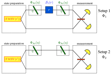
Figure 1: (Color online) Theoretical scheme of a specific example of channels satisfying Eq.s (10) and (11) proving the existence of Gaussian amendable maps. In both cases a TMSV state is prepared. In Setup 1 the channel $\Phi_{1}$ is applied to one part of the state, while in setup 2 the channel $\Phi_{2}$ is used. By measuring the entanglement of output state one can check for which set of parameters $\Phi_{1}$ is EB while $\Phi_{2}$ is not EB.

The theoretical model of this test is graphically depicted in Fig. 1, where we sketch the scheme of $\Phi_{1}$ and $\Phi_{2}$. In both cases the map is applied to one side of a TMSV state with squeezing parameter $r^{\prime}$ (see Eq. (4)). After the application of $\Phi_{1}$ it has been proved (see Fig. 4a of Ref. amendableChTEO ) that there exists a range of $\eta$ for which the output state is separable. On the other hand, when $\Phi_{2}$ is applied the output state is always entangled, for all values of $r^{\prime}$ and $\eta$ (see Fig. 4b of Ref. amendableChTEO ). The equivalence between Eq.s (10,11) and Eq.s (8,9) implies that the Gaussian map $\Phi=\mathcal{S}(r)\circ\Phi_{At}(\eta)$ is amendable via a squeezing unitary filter $\mathcal{S}^{\dagger}(r)$. This theoretical scheme will be our starting point for designing a more realistic experimental proposal.

III Experimental proposal

In this section we propose an experimental set–up in order to realize an effective amendable Gaussian map, endowed with the appealing property of being quite simple to be realized in the laboratory. Furthermore, we will also take into account the effects of losses, detection inefficiency and, eventually, measurement indeterminacy.

III.1 Preparation stage

Our starting point is the theoretical model given in Fig. 1. Notice that, even though appearing quite simple, the first set–up associated with the channel $\Phi_{1}$ in principle requires, in addition to the state preparation part, a non-trivial active operation on the system: the local squeezing between the two beam splitters. In quantum optics active operations can be realized by non-linear interactions. In most squeezing schemes, the initial state (e.g. vacuum, coherent, squeezed and/or thermal) interacts with a strong classical field in an optical nonlinear medium. This can be achieved for example by a sub–threshold optical parametric oscillator (OPO) squeezedOPO . Compared with passive transformations, active operations are relatively difficult to be engineered and experimentally costly. In order to get around this obstacle, our idea is to use a single initial active operation both for the generation of the entangled (probe) state and for the (indirect) realization of the local squeezing. These resources will be obtained in the preparation stage described in Fig. 2.

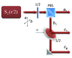
Figure 2: (Color online) Experimental scheme for the generation of the resource states. A type II OPO gives a twin beam described by the covariance matrix (4). The entangled modes $a$ and $b$ are orthogonally polarized. By applying a $\lambda/2$ wave plate and a polarizing beam splitter (PBS) to $a$ and $b$, we can obtain two independent single mode squeezed vacuum states $a_{1}$ and $b_{1}$ with orthogonal squeezing phases (Eq. (14)). Then, through a balanced beam splitter (the red one), polarization insensitive, we mix mode $b_{1}$ with the vacuum state $v$ obtaining the pair $\left(c_{1},c_{2}\right)$, a pure TMSV (Eq. (III.1)). This pair represents the entangled system on which we will test the entanglement–breaking properties of the maps $\Phi_{1}$ and $\Phi_{2}$ defined in Eq.s (12,13). The pure single mode beam $a_{1}$ will be used for implementing the squeezing transformation $\mathcal{S}(r)$.

At the output of a type II OPO one has at disposal two cross-polarized but frequency degenerate entangled modes PRL2009 , say $a$ and $b$. As shown in Fig. 2, by means of a $\lambda/2$ wave plate and a polarizing beam–splitter (PBS) it is possible to manipulate the entangled state in order to obtain two independent single-mode squeezed vacuum states JOB2005 $a_{1}$ and $b_{1}$, with orthogonal squeezing phases. According to the notation introduced in Section II.1, the correlation matrix of the latter modes can be written as

$${V}^{a_{1},b_{1}} = B(1/2)V_{2}^{a,b}(r^{\prime})B(1/2)$$ (14)

$$= V_{1}^{a}(r^{\prime})\oplus V_{1}^{b}(-r^{\prime}\ )\,.$$

Then, combining the mode $b_{1}$ with the vacuum $v$ by means of a balanced polarization insensitive beam splitter (the red plate in Fig. 2 with $\eta=1/2$), we generate the pair of modes $c_{1},c_{2}$ with correlation matrix

$$V^{c_{1},c_{2}} = B\left(\frac{1}{2}\right)[V_{1}^{b_{1}}(-r)\oplus V_{0}]B\left(\frac{1}{2}\right)$$

$$= [S(-\frac{r}{4})\oplus S((-\frac{r}{4})]V_{2}(-\frac{r}{2})[S((-\frac{r}{4})\oplus S((-\frac{r}{4})]\,.$$

Notice that, up to local (single-mode) operations, $c_{1}$ and $c_{2}$ are in a TMSV state with squeezing parameter $r^{\prime}=-r/2$, i.e. half of the original two–mode squeezing characterizing the pair $a$ and $b$ at the OPO output. At the same time, we will have at disposal an auxiliary single–mode squeezed vacuum $a_{1}$ that, in a certain sense, carries the second half of the original squeezing.

Summarizing, at the output of the above described generation stage we have at disposal three optical modes: the entangled pair $c_{1},c_{2}$, which will play the role of the probe state for testing the entanglement–breaking properties of the Gaussian maps $\Phi_{1}$ and $\Phi_{2}$, and the squeezed mode $a_{1}$ which will be used as a resource for mimicking a single-mode squeezer. We expect that suitably setting the OPO squeezing $r$ and the beam splitters transmissivity $\eta$, we can find that the final state, of the pair $(c_{1},\,c_{2})$, is separable under the action of $\Phi_{1}$ and entangled for $\Phi_{2}$.

III.2 Channel stage

In this Section, we will show how to implement the maps $\Phi_{1}$ and $\Phi_{2}$ defined in Eq.s (12,13), and graphically represented in Fig. 1.

Let us first consider $\Phi_{1}$. As recalled in Section II.1, each attenuation map $\Phi_{At}(\eta)$ can be directly implemented by letting the incoming mode pass through a beam splitter of transmissivity $\eta$. Less trivial is the passive implementation of the local squeezing $\mathcal{S}(r)$ without using another OPO. This can be indirectly achieved mixing the auxiliary squeezed mode $a_{1}$ with $c_{1}$ onto a beam splitter of transmissivity $\eta$. As a matter of fact, by observing that

$$[S(r)\oplus S(r)]B(\eta)=B(\eta)[S(r)\oplus S(r)]\,,$$ (16)

it derives that combining an incoming mode with a single mode squeezed vacuum on a beam splitter is equivalent to indirectly attenuating and then squeezing the system, as graphically shown in Fig. 3.

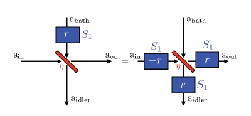
Figure 3: (Color online) Graphical representation of the equivalence between mixing a single mode squeezing and a generic state onto a beam splitter of a given transmissivity $\eta$ and a more complex operation consisting in the sequence $\mathcal{S}(r)\circ\Phi_{At}\circ S(-r)$. In both case the idler mode is traced out. This shows how a squeezed ancilla mode can be used to effectively realize a squeezing operation on a given input state.

More precisely, we have that the effect of the first optical circuit of Fig. 3, tracing out the idler mode, is equivalent to the sequence

$$\mathcal{S}(r)\circ\Phi_{At}\circ S(-r).$$ (17)

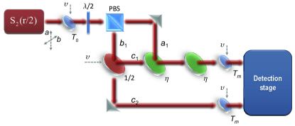
Figure 4: (Color online) Full scheme composed by the preparation stage (see Fig. (2)) followed by the implementation of $\Phi_{1}$ and $\Phi_{2}$ by means of two BSs with transmissivity $\eta$ (lower right corner of the picture). Three fictitious BSs, see Sec. IV A, mimic the effects of losses (BS with transmissivity $T_{0}$) and detection inefficiencies (BSs with transmissivity $T_{m}$).

By applying this equivalence property, we can easily implement the action of $\Phi_{1}$ on the incoming mode $c_{1}$, as pictorially represented in the full experimental set–up given in Fig. 4. Here the green beam splitters act on the incoming mode $c_{1}$ as

$$\Phi_{At}\circ\mathcal{S}(r)\circ\Phi_{At}\circ S(-r)=\Phi_{1}\circ S(-r)\,,$$ (18)

thus experimentally realizing the map of Eq.(12) up to the unitary transformation $S(-r)$. We recall that the entanglement-breaking properties of a map, are invariant under unitary redefinition of the input and output spaces EBT , that is $\Phi_{1}\circ S(-r)\in\mathrm{EB}$ iff $\Phi_{1}\in\mathrm{EB}$.

On the other hand, the implementation of the channel $\Phi_{2}$ defined in Eq. (13) can be straightforwardly implemented by discarding the auxiliary mode $a_{1}$ and substituting it with the vacuum. In other words, one should simply let the mode $c_{1}$ pass through the green beam splitters without feeding any light in the empty ports.

We can therefore conclude that the experimental setup represented in Fig.  4 is, up to experimental losses, equivalent to the theoretical scheme in Fig. 1. For the sake of clearness, let us point out that while in the theoretical scheme of Fig. 1 the squeezing parameters $r^{\prime}$ and $r$ are totally independent, in the realistic setup of Fig. 4 the structure of the scheme forces $r^{\prime}=-r/2$. Nonetheless, this lack of freedom does not affect the feasibility of the experiment.

IV Effective channel properties

As explained in Section II.2 (see Eq.s (10-13)), in order to experimentally prove the existence of Gaussian amendable channels we need to show that $\Phi_{1}$ is entanglement-breaking while $\Phi_{2}$ is not. This can be done by measuring the output state of our experimental circuit and checking its separability for different choices of the experimental parameters. In particular we will apply the PPT criterion PPT01 ; PPT02 ; PPT03 to the CM of the output state.

Here we discuss the proposed experimental scheme and we theoretically estimate $V^{out}$, the expected CM for the final state. By writing it in $2\times 2$ blocks

$$V^{out}=\begin{pmatrix}\mathbf{A}&\mathbf{C}\\ \mathbf{C^{\top}}&\mathbf{B}\end{pmatrix}\,,$$ (19)

one can easily compute the minimum symplectic eigenvalue $\nu$ of the partially transposed state

$$\nu=\sqrt{\frac{\Sigma-\sqrt{\Sigma^{2}-4\det[V^{out}]}}{2}}$$ (20)

where $\Sigma=\det[\mathbf{A}]+\det[\mathbf{B}]-2\det[\mathbf{C}]$. From the PPT criterion it can be shown that the output state is entangled if and only if

$$\nu^{2}<\frac{1}{4}$$ (21)

(see gaussian03 and references therein). The relation above, provides a necessary and sufficient criterion for testing the separability of the output state and thus for studying the entanglement-breaking properties of the applied map.

The behaviour of $\nu^{2}(\eta)$ for initial squeezing $\left|r\right|=1.3$ is given in Fig. 5, that refers to the case of ideal (lossless) preparation stage and detectors with unit efficiency. It results that, if on the one hand $\Phi_{2}$ can never become ${\mathrm{EB}}$ for any value of the transmissivity $\eta$ (i.e. $\nu^{2}$ is always lower than $1/4$ so that the state keeps its entanglement), on the other hand there exists a finite interval of $\eta$ such that $\Phi_{1}\in{\mathrm{EB}}$ and thus its output state is separable. This separability interval has been computed in amendableChTEO and corresponds to $\eta\leq\tilde{\eta}(r^{\prime})$ with

$$\tilde{\eta}(r^{\prime})=\frac{1}{2}\left(\cosh(2r^{\prime})-\sqrt{2\cosh(2r^{\prime})-1}\right)\text{csch}^{2}(r^{\prime})\,.$$ (22)

In the next subsection, we will consider the effects of losses, detection inefficiencies and measurement uncertainties.

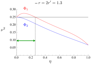
Figure 5: (Color online) Entanglement witness parameter $\nu^{2}$ as a function of the transmissivity $\eta$, computed for the outcomes of $\Phi_{1}$ and $\Phi_{2}$, in absence of losses and noise. As expected, $\Phi_{2}$ preserves the entanglement of the incoming twin-beam for all $\eta$, indeed $\nu^{2}<1/4$ (as signaled by the lower (blue) curve). On the other hand, there exists a finite interval of transmissivity such that the output state of $\Phi_{1}$ is separable ($\nu^{2}>1/4$).

IV.1 Measurement uncertainty, losses and inefficiencies

In a realistic implementation we cannot neglect the statistical uncertainty affecting the measurement process and, at the same time, we also have to consider the effects of losses (decoherence) and detection efficiency.

In order to take into account the experimental indeterminacy into Eq. (20) we have considered typical experimental values for the uncertainties relative to the CM elements. These values are used in propagating the measurement’s errors into the formula that gives $\nu^{2}$ in terms of CM elements (a detailed discussion on the errors affecting the different elements can be found in Ref. JOSAB2010 ). Thus we obtain the statistical error $\delta(\nu^{2})$ for $\nu^{2}$. From the experimental point of view claiming that $\Phi_{1}\in{\mathrm{EB}}$ requires that $\nu_{\Phi_{1}}^{2}-1/4>2\delta(\nu^{2})$, i.e. the distance from the separability threshold must overcome the measurement confidence interval (i.e. twice the uncertainty).

In Fig. 6 we have fixed $r^{\prime}=-r/2=0.5$ and plotted $\nu^{2}$ as a function of $\eta$. The dashed lines represent the boundaries of the confidence interval for $\nu^{2}$. From this plot we conclude that in this case the confidence interval $2\delta(\nu^{2})$ would make ambiguous, from the experimental point of view, the statement that $\Phi_{1}\in{\mathrm{EB}}$. This ambiguity can be overcome by considering an increased level of the squeezing for the pure state generated by the type–II OPO. For example, it is sufficient to raise $|r|$ from $1$ to $1.3$ to obtained a clear experimental proof that $\Phi_{1}\in{\mathrm{EB}}$ for $\eta\leq\tilde{\eta}$, as shown in Fig. 6. Here $\nu^{2}\left(\eta\right)$ is plotted for $r^{\prime}=-r/2=0.65$, and $\nu_{\Phi_{1}}^{2}-1/4$ is greater than the expected confidence interval in a range of values for $\eta$ contained in $[0,\tilde{\eta}]$.

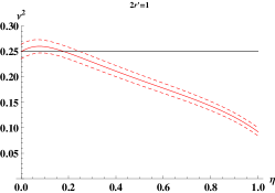
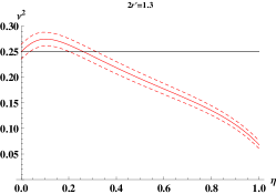
Figure 6: (Color online)Entanglement witness parameter $\nu^{2}$ as a function of $\eta$ for two different values of the squeezing parameter associated to the initial modes $a$ and $b$: $r^{\prime}=-r/2=0.5$ in (a) and $r^{\prime}=-r/2=0.65$ in (b). The dashed lines indicate the confidence interval one should expect for $\nu^{2}$ in a typical measurement of the covariance matrix elements via homodyne detection.

Furthermore, real experiments face the effects of absorption losses and non–ideal detection, which can be modeled by the three fictitious beam splitters we have introduced in Fig. 4. The first one of transmissivity $T_{0}$ (on the left) simulates the effects of losses and in particular, the OPO cavity escape efficiency PRL2009 that unavoidably makes any state at the output of an OPO cavity a mixed one mixed . The last two beam splitters of transmissivity $T_{m}$ (on the right) model the inefficiency of the detectors.

It is interesting to see that the conclusions retrieved from the analysis performed in Fig. 6 are still valid if losses and detection inefficiencies are taken into account. In Fig. 7 we plot the behavior of $\nu^{2}\left(\eta\right)$ in a realistic scenario, setting the losses at $25\%$ so that $T_{0}=0.75$ and detection efficiency at $T_{m}=0.90$, and assuming the same statistical indeterminacy used in the case without losses. The effect of $T_{0}<1$ and $T_{m}<1$ is, on one hand, to reduce the maximum value for $\nu^{2}$ inside the EB region (the maximum also moves to a higher $\eta$’s value), on the other hand, to enlarge the $\eta$ interval for which $\Phi_{1}=\Phi^{2}\in{\mathrm{EB}}$.

We note that while reducing the weight of losses and detection inefficiencies is surely possible ($T_{0}=0.95$ and $T_{m}=0.97$ have been recently reported Schnabel2013 ) experimental indeterminacy cannot be avoided and, as far as we know, the value used in Ref. JOSAB2010 is the lowest one for the experimental determination of the CM of a bipartite Gaussian state.

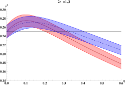
Figure 7: (Color online) Entanglement witness parameter $\nu^{2}$ as a function of $\eta$. We have fixed the squeezing parameter associated to the initial modes $a$ and $b$ to $r^{\prime}=-r/2=0.65$. We compare the ideal case (no-loss and unit detection efficiency, red line) with a realistic case where $T_{0}=0.75$ and $T_{m}=0.90$ (blu dashed line). The plotted lines correspond to the expectation values while shadowed areas encompass confidence intervals. The plot, clearly, shows that the proposed scheme is quite insensitive to losses and detection inefficiency.

V Conclusions

In this work we have proposed a realistic quantum optics experiment based on continuous variable systems that would provide the existence of Gaussian amendable maps and give more insight on entanglement breaking channels from a practical point of view.

The proposed scheme is translated into a rather simple experimental set–up. Indeed, it is based on a single initial non-linear operation (realized by a type–II sub–threshold OPO) which has the role of preparing both the input entangled state and a squeezed ancilla. The rest of the scheme is extremely simple since it requires only passive operations such as beam splitters and wave-plates.

The proposal has been realistically analyzed by taking into account the typical statistical uncertainty of Gaussian state quantum homodyne tomography. The effects of losses and detector inefficiencies have also been considered. We have shown that, even in presence of such errors and losses, the experiment is still feasible. Indeed, a conclusive test can be achieved by appropriately tuning the experimental parameters. The proposed scheme can be readily implemented in any laboratory having at disposal a running source of bipartite Gaussian entangled states.

References

- (1) W. H. Zurek, ”Decoherence, einselection, and the quantum origins of the classical”, Rev. Mod. Phys. 75, 715–775 (2003);
- (2) M. A. Nielsen and I. L. Chuang, Quantum Computation and Quantum Information, (Cambridge University, 2000);
- (3) A. Serafini, M. G. A. Paris, F. Illuminati, and S. De Siena, ”Quantifying decoherence in continuous variable systems ” J. Opt. B: Quantum Semiclass. Opt. 7, R19–R36 (2005);
- (4) D. Buono, G. Nocerino, A. Porzio, and S. Solimeno, ”Experimental analysis of decoherence in continuous-variable bipartite systems”, Phys. Rev. A 86, 042308 (2012);
- (5) R. Horodecki, P. Horodecki, M. Horodecki, and K. Horodecki, ”Quantum entanglement” Rev. Mod. Phys. 81, 865–942 (2009);
- (6) O. Gühne and G. Tóth, ”Entanglement detection”, Phys. Rep. 474, 1–75 (2009);
- (7) M. Horodecki, P. W. Shor, M. B. Ruskai, ”General Entanglement Breaking Channels”, Rev. Math. Phys. 15, 629–641 (2003);
- (8) A. S. Holevo, ”Quantum coding theorems”, Russian Math. Surveys, 53, 1295–1331 (1999);
- (9) A. S. Holevo, M. E. Shirokov and R. F. Werner, ”On the notion of entanglement in Hilbert spaces” Russ. Math. Surv. 60, 359–360 (2005);
- (10) A. S. Holevo, ”Entanglement-Breaking Channels in Infinite Dimensions ”, Problems of Information Transmission 44, 171–184 (2008);
- (11) A. De Pasquale and V. Giovannetti, ”Quantifying the noise of a quantum channel by noise addition”, Phys. Rev. A 86, 052302 (2012);
- (12) H.-J. Briegel, W. Dür, J. I. Cirac, and P. Zoller, Phys. Rev. Lett. 81, 5932 (1998);
- (13) L.-M. Duan, M. D. Lukin, J. I. Cirac, and P. Zoller, Nature 414, 413 (2001);
- (14) N. Sangouard, C. Simon, J. Minář, H. Zbinden, H. de Riedmatten, and N. Gisin, Phys. Rev. A 76, 050301(R) (2007).
- (15) A. S. Holevo and R. F. Werner, ”Evaluating capacities of bosonic Gaussian channels”, Phys. Rev. A 63, 032312 (2001);
- (16) J. Eisert and M. M. Wolf, ”Gaussian quantum channels” in Quantum Information with Continous Variables of Atoms and Light, N.J. Cerf, G. Leuchs, and E.S. Polzik eds. (Imperial College Press, London, 2007), pp. 23–42;
- (17) C. Weedbrook, S. Pirandola, R. García-Patrón, N. J. Cerf, T. C. Ralph, J. H. Shapiro, and S. Lloyd, ”Gaussian Quantum Information” Rev. Mod. Phys. 84, 621–669 (2012);
- (18) S. Olivares, ”Quantum optics in the phase space - A tutorial on Gaussian states” Eur. Phys. J. Special Topics 203, pp. 3–24 (2012);
- (19) A. S. Holevo and V. Giovannetti, ”Quantum channels and their entropic characteristics”, Rep. Prog. Phys. 75, 046001 (2012);
- (20) S. L. Braunstein and P. Van Loock, ”Quantum information with continuous variables” Rev. Mod. Phys. 77, 513–577 (2005);
- (21) C. M. Caves and P. D. Drummond, ”Quantum limits on bosonic communication rates” Rev. Mod. Phys. 66, 481–537 (1994).
- (22) A. De Pasquale, A. Mari, A. Porzio, and V. Giovannetti, ”Amendable Gaussian channels: Restoring entanglement via a unitary filter”, Phys. Rev. A, 87, 062307 (2013);
- (23) V. D’Auria, S. Fornaro, A. Porzio, S. Solimeno, S. Olivares, and M. G. A. Paris, ”Full Characterization of Gaussian Bipartite Entangled States by a Single Homodyne Detector”, Phys. Rev. Lett. 102, 020502 (2009).
- (24) V. D’Auria, S. Fornaro, A. Porzio, E. A. Sete, and S. Solimeno, ”Fine tuning of a triply resonant OPO for generating frequency degenerate CV entangled beams at low pump powers”, Appl. Phys. B 91, 309–314 (2008).
- (25) A. S. Holevo “Probabilistic and Statistical Aspects of Quantum Theory” 2nd ed. (Edizioni della Normale, Pisa 2011).
- (26) F. Caruso, V. Giovannetti, and A. S. Holevo, ”One-mode bosonic Gaussian channels: a full weak-degradability classification”, New J. Phys. 8, 310 (2006);
- (27) V. D’Auria, A. Porzio, S. Solimeno, S. Olivares, and M. G. A. Paris, ”Characterization of bipartite states using a single homodyne detector”, J. Opt. B: Quantum Semiclass. Opt. 7, S750–S753 (2005);
- (28) L.-An Wu, H. J. Kimble, J. L. Hall, and H. Wu, ”Generation of Squeezed States by Parametric Down Conversion”, Phys. Rev. Lett. 57, 2520–2523 (1986);
- (29) A. Peres, ”Separability Criterion for Density Matrices”, Phys. Rev. Lett. 77, 1413–1415 (1996);
- (30) P. Horodecki, ”Separability criterion and inseparable mixed states with positive partial transposition”, Phys. Lett. A 232, 333–339 (1997);
- (31) R. Simon, ”Peres-Horodecki Separability Criterion for Continuous Variable Systems”, Phys. Rev. Lett. 84, 2726–2729 (2000);
- (32) D. Buono, G. Nocerino, V. D’Auria, A. Porzio, S. Olivares, and M. G. A. Paris, ”Quantum characterization of bipartite Gaussian states”, J. Opt. Soc. Am. B, 27, A110–A118 (2010);
- (33) V. D’Auria, C. de Lisio, A. Porzio, S. Solimeno, and M. G. A. Paris, ”Transmittivity measurements by means of squeezed vacuum light”, J. Phys. B: At. Mol. Opt. Phys. 39, 1187–1198 (2006);
- (34) S. Steinlechner, Jöran Bauchrowitz, T. Eberle, and R. Schnabel, ”Strong Einstein-Podolsky-Rosen steering with unconditional entangled states”, Phys. Rev. A 87, 022104 (2013).