On oscillations of solutions of the fourth-order thin film equation near heteroclinic bifurcation point

Abstract.

The behaviour of solutions of the Cauchy problem for the 1D fourth-order thin film equation (the TFE–4)

$$u_{t}=-(|u|^{n}u_{xxx})_{x}\quad\mbox{in}\quad\mathbb{R}\times\mathbb{R}_{+},$$

where, mainly, $n\in(\frac{3}{2},2]$, is studied. Using the standard mass-preserving (ZKB-type) similarity solution of the TFE–4, a third-order ODE for the profile $f(y)$ occurs:

$$\begin{matrix}u_{\rm s}(x,t)=t^{-\frac{1}{4+n}}f(y),\,\,\,y=\frac{x}{t^{1/(4+n)}}\quad\Longrightarrow\quad-(|f|^{n}f^{\prime\prime\prime})^{\prime}+\frac{1}{4+n}\,(yf)^{\prime}=0\vskip 3.0pt plus 1.0pt minus 1.0pt\\ \quad\Longrightarrow\quad-|f|^{n}f^{\prime\prime\prime}+\frac{1}{n+4}\,yf=0.\end{matrix}$$

For the Cauchy problem, the oscillatory behaviour of $f(y)$ near the interface was studied in [13, 16], etc. It was shown that a periodic oscillatory component $\varphi(s)$, describing the actual sign-changing behaviour of $u_{\rm s}(x,t)$ close to finite interfaces, exists up to a critical homoclinic bifurcation exponent $n_{\rm h}$, i.e., for

$$0<n<n_{\rm h}\in(\frac{3}{2},n_{\rm+}),\quad\mbox{where}\quad n_{\rm+}=\frac{9}{3+\sqrt{3}}=1.9019238...\,.$$

Careful numerics show that $n_{\rm h}=1.75987...\,.$

In the present paper, a non-oscillatory behaviour of $f(y)$ for $n\in[n_{\rm h},2]$, i.e., above the heteroclinic value, is revealed by a combination of analytical and numerical methods. In particular, this implies that, for $n\in[n_{\rm h},2]$ (and, at least, up to $3$), the Cauchy setting coincides with the standard zero-height-angle-flux free-boundary one (with non-negative solutions), studied in detail in many well-known papers since the end of 1980s, including Bernis–Friedman’s seminal paper [2] of 1990.

1. Introduction: TFE–4, first similarity solution, and main result

1.1. The TFE–4 and first mass-preserving similarity solution

We study the first mass-preserving self-similar solution of the fourth-order thin film equation (the TFE–4) in one dimension

(1.1) $$u_{t}=-(|u|^{n}u_{xxx})_{x}\quad\mbox{in}\,\,\,\mathbb{R}\times\mathbb{R}_{+},$$

where, in the most of the cases, $n\in(\frac{3}{2},2]$ is a fixed exponent. Equation (1.1) is written for solutions of changing sign, which is an essential feature for the Cauchy problem (CP) to be considered, though, in a supercritical parameter $n$-range (see below), solutions turn out to be non-negative, as happens for the standard and much more well-studied (at least, since 1980s) free-boundary problem (FBP) with zero-height, zero-contact angle, and zero-flux conditions; see references in [13] and in several other papers mentioned below.

Thus, we will need well-known similarity solutions of the TFE–4 (1.1). Source-type mass-preserved (i.e., of a ZKB-type) similarity solutions of the FBP for (1.1) for arbitrary $n$ were studied in [6] for $N=1$ and in [15] for the equation in $\mathbb{R}^{N}$. More information on similarity and other solutions can be found in [1, 3, 4, 7, 9, 10]. TFEs admit non-negative solutions constructed by “singular” parabolic approximations of the degenerate nonlinear coefficients. We refer to the pioneering paper by Bernis and Friedman [2] (1990) and to various extensions in [11, 12, 18, 20, 19, 22, 23, 26] and the references therein. See also [21] for mathematics of solutions of the FBP and CP of changing sign (such a class of solutions of the CP will be considered later on).

In both the FBP and the CP, the source-type solutions of the TFE–4 (1.1) are

(1.2) $$\textstyle{u_{\rm s}(x,t)=t^{-\frac{1}{4+n}}f(y),\quad y=\frac{x}{t^{1/(4+n)}},}$$

where, on substitution of (1.2) into (1.1), $f(y)$ solves a divergent fourth-order ordinary differential equation (ODE):

(1.3) $$\textstyle{-(|f|^{n}f^{\prime\prime\prime})^{\prime}+\frac{1}{4+n}\,(yf)^{\prime}=0.}$$

On integration once, by using the continuity of the flux function $|f|^{n}f^{\prime\prime\prime}$ at the interface, where $f=0$, one obtains a simpler third-order ODE of the form

(1.4) $$\textstyle{|f|^{n}f^{\prime\prime\prime}=\frac{1}{4+n}\,yf.}$$

In view of existence of evident scaling, we, first, get rid of the multiplier $\frac{1}{4+n}$, and, next, pose the symmetry condition at the origin and the last normalizing one to get

(1.5) $$|f|^{n}f^{\prime\prime\prime}=yf\quad\mbox{for}\quad y>0,\quad\mbox{with}\quad f^{\prime}(0)=0,\quad\mbox{and}\quad f(0)=1.$$

Later on, for asymptotic expansions close to the interface point, assuming that such a solution has its interface as some finite $y_{0}>0$ (so that $f(y)\equiv 0$ for $y\geq y_{0}$), we perform a reflection,

(1.6) $$y-y_{0}\mapsto y\quad\Longrightarrow\quad|f|^{n}f^{\prime\prime\prime}=-(y_{0}-y)f\quad\mbox{for small}\quad y>0.$$

From now on, we will mainly concentrate on solutions and the corresponding profiles $f(y)$ for the Cauchy problem only, though, for some supercritical range from $n\in\big{(}\frac{3}{2},2\big{]}$ and even further, as will turn out, we will conclude that this covers the FBP setting as well.

For the Cauchy problem, it was formally shown that there exists an oscillatory similarity profile of (1.3), that are infinitely oscillatory as $y\to y_{0}^{-}$, for not that large exponents

(1.7) $$n\in(0,n_{\rm h}),\quad\mbox{where}\quad n_{\rm h}=1.75987...;$$

see [13]. For $n\in(0,1)$, existence and uniqueness (up to the mass-scaling) of an oscillatory $f(y)$ are straightforward consequences of the result in [5] on oscillatory solutions for the fully divergent fourth-order porous medium equation; see (2.4) below. See also some details in [17, § 3.7] and interesting oscillatory features of similarity dipole solutions of the TFE (1.1) observed in [8]. Stability of such sign changing similarity solutions is quite plausible but was not proved rigorously being an open problem.

Thus, in the present paper, we concentrate on the still unknown parameter range

(1.8) $$n\in[n_{\rm h},2].$$

Our main goal is to show that, in this parameter range, the above similarity solutions, as solutions of the Cauchy problem, are not oscillatory, and, moreover, do not change sign in small neingbourhoods of finite interfaces. In addition, we then claim that, for such $n$’s in (1.8), similarity (and, most plausibly, not only those) solutions of the CP and the FBP (see a number of papers mentioned above) coincide.

2. Heteroclinic subcritical and supecritical ranges

We begin with a brief explanation of known results on what happens in the heteroclinic subcritical range (1.7), which is important for our final conclusions.

2.1. Local oscillatory structure near interfaces for $n\in(0,n_{\rm h})$

Namely, it is known that the asymptotic behaviour of $f(y)$ satisfying equation (1.4) near the interface point as $y\to y_{0}^{-}>0$ is given by the expansion

(2.1) $$f(y)=(y_{0}-y)^{\mu}\varphi(s),\quad s=\ln(y_{0}-y),\quad\mu=\frac{3}{n},$$

where, on substitution to (1.5), after scaling, the oscillatory component $\varphi$ satisfies the following autonomous ODE, where an exponentially small as $s\to-\infty$ term (occurring by setting $y=y_{0}-{\mathrm{e}}^{s}$) is omitted:

(2.2) $$\textstyle{\varphi^{\prime\prime\prime}+3(\mu-1)\varphi^{\prime\prime}+(3\mu^{2}-6\mu+2)\varphi^{\prime}+\mu(\mu-1)(\mu-2)\varphi+\frac{\varphi}{|\varphi|^{n}}=0.}$$

It was shown that here exists a stable (as $s\to+\infty$) changing sign periodic solution $\varphi_{*}(s)$ of (2.2). The bifurcation value $n_{\rm h}$ was obtained in [13] by some analytic and numerical evidence showing that, as $n\to n_{\rm h}^{-}$, the ODE (2.2) exhibits a usual heteroclinic bifurcation, where a periodic solution is generated from a heteroclinic path of two constant equilibria, [24, Ch. 4]. According to (2.1), this gives similarity profiles of changing sign, which being extended by $f(y)\equiv 0$ for $y>y_{0}$ form a compactly supported solution $f\in C^{\alpha}$ in a neighbourhood of $y=y_{0}$, with $\alpha\sim\frac{3}{n}$. Notice that $\alpha\to+\infty$ as $n\to 0^{+}$, so the regularity at $y=y_{0}$ improves to $C^{\infty}$ at $n=0^{+}$ (and eventually, to an analytic profile $F(y)$ for $n=0$ for all $y>0$, being the “Gaussian” kernel of the fundamental solution $b(x,t)=t^{-\frac{1}{4}}F(x/t^{\frac{1}{4}})$ of the linear parabolic operator $D_{t}+D_{x}^{4}$).

Remark: TFE in $\mathbb{R}^{N}$. The above conclusions, at least, formally can be applied to the Cauchy problem for the TFE–4 in $\mathbb{R}^{N}$:

(2.3) $$u_{t}=-\nabla\cdot(|u|^{n}\nabla\Delta u)\quad\mbox{in}\quad\mathbb{R}^{N}\times\mathbb{R}_{+},$$

with a bounded compactly supported data $u_{0}(x)$. Namely, at any point of a sufficiently smooth interface surface, at which there exists a unique tangent hyperplane $\pi$, the same 1D oscillatory behaviour is expected to occur in the direction of the inward unit normal to $\pi$. In other words, the principal phenomenon of existence of oscillatory sign-changing behaviour near the smooth interfaces is essentially 1D, excluding some special and “singular” non-generic cases.

On the other hand, at possible points of singular “cusps” at the interfaces (anyway, expected to be non-generic), such an easy approach is not applicable, though almost nothing is known about those singular phenomena for (2.3) for any $N\geq 2$.

Note that the first results on the oscillatory behaviour of similarity profiles for fourth-order ODEs related to the source-type solutions of the divergent parabolic PDE of the porous medium type (the PME–4)

(2.4) $$u_{t}=-(|u|^{m-1}u)_{xxxx}\quad(m>1)$$

were obtained in [5]. It turns out that these results can be applied to the rescaled TFE (1.3), but for $n\in(0,1)$ only. As shown in [13], the corresponding ODEs for source-type similarity solutions for (1.1) and (2.4) then coincide after a change of parameters $n$ and $m$:

$$m=\frac{1}{1-n},\quad n\in(0,1).$$

Some results on existence and multiplicity of periodic solutions of ODEs such as (2.2) are known [13], and often lead to a number of open problems. Therefore, numerical and some analytic evidence remain key, especially for sixth and higher-order TFEs; see [14] and [17, Ch. 3].

Returning to the behaviour as $s\to-\infty$ for (2.2), i.e., approaching the interface, we express the above results as follows: in the heteroclinic subcritical range, there exists a 2D bundle of asymptotic solutions of (2.2) in $\mathbb{R}$ having the expansion (2.1) (an exponentially small term is again omitted)

(2.5) $$f(y)=(y_{0}-y)^{\frac{3}{n}}[\varphi_{*}(s+s_{0})+...],\quad\mbox{with parameters $y_{0}>0$ and $s_{0}\in\mathbb{R}$},$$

where we take into account the phase shift $s_{0}$ of the periodic orbit $\varphi_{*}(s)$. Here, we should treat $y_{0}$ as a free parameter, though, in the above setting, it is fixed by conditions at $y=0$. Recall that, as $s\to-\infty$, the periodic solution $\varphi_{*}(s)$ is thus unstable by the obvious reason: a 1D unstable manifold is then generated by small perturbations of $y_{0}$.

Therefore, matching the 2D bundle (2.5) with two symmetry conditions at the origin in (1.5) leads to a formally well-posed problem of 2D matching. However, using this matching approach directly is a difficult open problem (for $n\in(1,n_{\rm h})$, where existence of $f(y)$ was not properly proved; recall that, for $n=1$, there is a pure algebraic approach to construct such a unique oscillatory profile [13]). Note that, in the case of an analytic dependence on parameters involved, such a problem cannot possess more than a countable set of isolated solutions.

2.2. $n\in(\frac{3}{2},2]$: numerical results

Before deriving proper asymptotic expansions in the supercritical range in the next section, we present some numerical evidence that, at $n=n_{\rm h}$, oscillations of $f(y)$, as a solution of (1.5), near the interface disappear.

As usual, for numerics, we use the regularization in the third-order operator in (1.5) by replacing

(2.6) $$|f|^{n}\mapsto(\varepsilon^{2}+f^{2})^{\frac{n}{2}},\quad\mbox{with}\quad\varepsilon=10^{-11},$$

which is sufficient for the accuracy required; see below. Note that, for our purposes in the Cauchy problem, we principally cannot use the pioneering FBP-regularization, introduced in Bernis–Friedman [2] (not analytic as in (2.6), except $n=2$, to be treated specially), leading, in many cases, to non-negative solutions. However, we expect that, for $n\in[n_{\rm h},2]$, both analytic and non-analytic $\varepsilon$-regularizations lead to the same solutions, i.e., the Cauchy and FBP settings coincide (though proving that rigorously is very difficult).

In our numerics by the MatLab, we were often obliged to keep a high accuracy, with both tolerancies $\sim 10^{-12}$, and the total number of points on the interval $y\in(0,3)$ of about 50000–100000, though using the simplest ODE solver for the Cauchy problem ode45 took, sometimes, 5–10 minutes for each shooting from $y=0$ for each fixed value of $n$.

There appears a simple one-parameter shooting problem for the ODE (1.5) from $y=0$ with the only parameter

(2.7) $$f^{\prime\prime}(0)=\mu\in\mathbb{R}.$$

Then, varying $\mu<0$, we are trying to approach as close as possible to the corresponding finite interface at some $y_{0}>0$, and, eventually, to see whether $f(y)$ changes sign or not in a small vicinity of $y_{0}^{-}$. A few of such results are presented below.

Thus, let us begin with the oscillatory range (1.7). In Figure 1, our numerics catch a changing sign behaviour as $y\to y_{0}^{-}$ for $n=1.7<n_{\rm h}$. Our shooting from $y=0$, with $f(0)=1$, even with the above mentioned accuracy and with about $10^{5}$ points, allows us to see just a single zero near $y_{0}^{-}$. We do not think that, in a few minutes of PC time, as here, the next, to say nothing of other zeros of $f(y)$, near $y_{0}^{-}$ can be viewed by such a shooting.

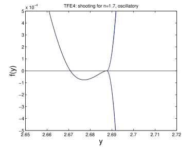
Figure 1. The first zero, close to $y=2.67$, of $f(y)$ near $y=y_{0}$ for $n=1.7$.

In the next Figure 2, we start to approach the heteroclinic bifurcation value $n_{\rm h}$ from below. Namely, we take $n=1.75$, which is still slightly less. We again were able to see the first zero, though to reach that, we increased the number of points, but still observed a “non-smooth” profile $f(y)$ close to the interface. We see that a negative hump in this figure, which is already of the order $\sim 10^{-7}$, so one can expect that further approaching $n_{\rm h}$ from below will require a completely different and more powerful computer tools.

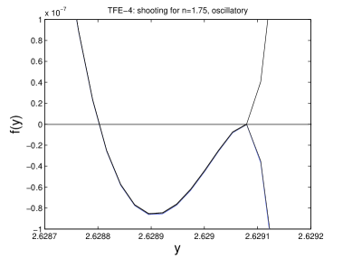
Figure 2. The first zero, close to $y=2.6288$, of $f(y)$ near $y=y_{0}$ for $n=1.75<n_{\rm h}$. Here, for the last profile, $f^{\prime\prime}(0)=-0.434097009$.

We next take $n$ very close to $n_{\rm h}$, where

(2.8) $$n=1.75987,\quad f^{\prime\prime}(0)=\mu=-0.435513146293,\quad y_{0}=2.6197.$$

In this case we enhance our numerics by taking 200000 points on the interval $(0,2.7)$ to get the results in Figure 3. Thus, up to the accuracy $10^{-7}$ (and more, as easily seen), $f(y)$ is not oscillatory for $y\approx y_{0}^{-}$, as our analytical predictions said earlier.

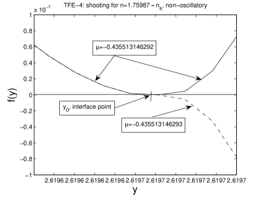
Figure 3. Non-oscillatory $f(y)$ near $y=y_{0}$ for $n=1.75987\approx n_{\rm h}^{-}$. Here, for the last profile, $\mu=f^{\prime\prime}(0)=-0.435513146293$.

Now, consider the supercritical range above $n_{\rm h}$. Figure 4, constructed for $n=1.8>n_{\rm h}$ (but rather close to it), shows that, with the prescribed accuracy, we do not see any sign changes near the interfaces, unlike the previous figures. In Figure 5, we show a global structure of this $f(y)$, which looks like being non-negative, but, to verify that, one needs more “microscopic” structure near the interface given in the previous figure.

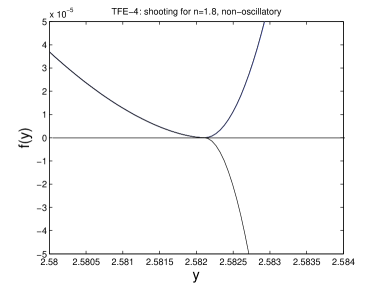
Figure 4. Non-oscillatory $f(y)$ for $n=1.8>n_{\rm h}$.

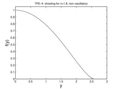
Figure 5. The non-oscillatory profile $f(y)$ for $n=1.8>n_{\rm h}$.

Finally, for completeness, in Figure 6, we present a full view of $f(y)$ for the special case $n=2$, where both analytic and non-analytic (for the FBP) regularizations coincide. Again, “microscopically”, no sign changes of $f(y)$ were observed.

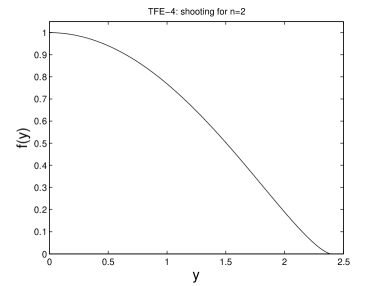
Figure 6. The non-negative profile $f(y)$ for $n=2$.

We do not expect (and did not see) any essential changes by further increasing $n\in(2,3)$ until the special $n=3$ to be treated next.

2.3. $n=3$: logarithmically perturbed linear asymptotics and existence of $f(y)$ for the CP

For $n=3$, similar to the case $n=\frac{3}{2}$ for the FBP, we observe a logarithmically perturbed linear asymptotics (we do not reveal the second term, since $n=3$ is currently out of our main interests): as $y\to y_{0}^{-}$,

(2.9) $$\textstyle{f(y)=\frac{3}{\sqrt{2}}\,(y_{0}-y)|\ln(y_{0}-y)|^{\frac{1}{3}}+...\,.}$$

The corresponding shooting of $f(y)$ is presented in Figure 7. Obviously, such similarity solutions with the expansion (2.9) do not satisfy the zero contact angle condition (however, other FBPs can be posed), but can be proper solutions of the Cauchy problem, so that this behaviour at interfaces can be that of a maximal regularity.

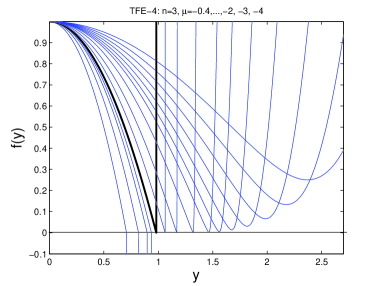
Figure 7. Non-oscillatory $f(y)$ for $n=3$, the bold-face line. For it, $\mu=f^{\prime\prime}(0)=-2.274...$  , $y_{0}=0.943...$  .

2.4. $n=4$: nonexistence of $f(y)$

As a simple illustration of the general results for the TFE–4 in [2], saying that solutions of this PDE are strictly positive for all $n$ large enough, consider our ODE (1.5) for the next integer $n=4$. The results of shooting from $y=0$ are shown in Figure 8: no solutions for $\mu=f^{\prime\prime}(0)$ from $-2$ to $-1000$ can reach the zero level $f=0$. It is clear that one does not need any proof (though it is already available in [2], and in much more general PDE fashion).

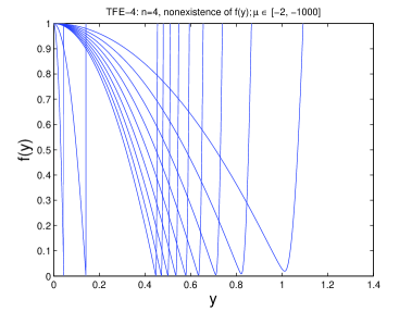
Figure 8. Nonexistence of $f(y)$ with a finite interface for $n=4$.

Anyway, as an ODE illustration again, we see from (1.6), $y_{0}=1$ by scaling, multiplying by $f^{\prime}$ and integrating that, keeping the main singular terms,

(2.10) $$\textstyle{f^{\prime}f^{\prime\prime}=\int(f^{\prime\prime})^{2}+\frac{1}{2}\,\frac{1}{f^{2}}+...\geq\frac{1}{2}\,\frac{1}{f^{2}}\,.}$$

However, the resulting “majorising” ODE

(2.11) $$\textstyle{f^{\prime}f^{\prime\prime}=\frac{1}{2}\,\frac{1}{f^{2}}}$$

does not admit increasing positive solutions for $y>0$ small (here, $y_{0}=0$ and $f(0)=0$, recall). Indeed, multiplying by $f^{\prime}$ and integrating yields:

(2.12) $$\textstyle{\frac{1}{3}\,(f^{\prime})^{3}=-\frac{1}{2}\,\frac{1}{f}+...<0\quad\mbox{for any small}\quad f>0.}$$

3. Positive expansions near interface for $n\in(\frac{3}{2},3)$

Thus, we consider the ODE (1.6) close to the interface $y_{0}=1$, by scaling. Assuming that $f(y)>0$ for small $y>0$ yields the following equation:

(3.1) $$f^{n-1}f^{\prime\prime\prime}=-1+y.$$

First of all, we cannot use the standard “parabolic” expansion from dozens of recent papers, since it is suitable for the FBP for $n\in(0,\frac{3}{2})$.

Therefore, we are looking for an expansion about a different profile (an explicit solution of (3.1) with $-1$ on the RHS):

(3.2) $$\textstyle{f_{0}(y)=B_{0}y^{m},\quad\mbox{where}\quad m=\frac{3}{n}\quad\mbox{and}\quad B_{0}^{n}=\big{[}\frac{3}{n}\big{(}\frac{3}{n}-1\big{)}\big{(}2-\frac{3}{n}\big{)}\big{]}^{-1},}$$

which makes sense for any

(3.3) $$\textstyle{n\in\big{(}\frac{3}{2},3\big{)}.}$$

We next use an algebraic perturbation of (3.2) by setting

(3.4) $$\textstyle{f(y)=B_{0}y^{m}+Dy^{l}+...,\quad\mbox{where}\quad l>m=\frac{3}{n}}$$

and $D\in\mathbb{R}$ is an arbitrary parameter (recall that we need a 1D bundle to shoot a single symmetry boundary condition $f^{\prime}(0)=0$). Substituting into (3.1) yields

(3.5) $$D[B_{0}^{n-1}(n-1)m(m-1)(m-2)+B_{0}l(l-1)(l-2)]\,y^{m(n-1)+l-3}=-y+...\,.$$

One can see that equating both algebraic functions on both sides of (3.5) is no good: this yields a unique orbit, and not a 1D bundle (see below). Therefore, the only possible way is to assume that

(3.6) $$\textstyle{m(n-1)+l-3<1\quad\Longrightarrow\quad\frac{3}{n}<l<1+\frac{3}{n},}$$

and equate to zero the square bracket on the LHS in (3.5). This gives the following cubically algebraic (“characteristic”) equation for the exponent $l$:

(3.7) $$\textstyle{l:\quad l(l-1)(l-2)=B_{0}^{n-2}(n-1)\frac{3}{n}\big{(}\frac{3}{n}-1\big{)}\big{(}2-\frac{3}{n}\big{)}.}$$

It is worth mentioning that a literal balancing $m(n-1)+l-3=1$ in (3.8) just means that $D=0$ in such an (3.4), i.e., this orbit also belongs to the above 1D bundle.

After simple transformations, this is reduced to the cubic equation

(3.8) $$\framebox{$\textstyle{l:\quad H_{n}(l)\equiv l(l-1)(l-2)-(n-1)\big{[}\frac{3}{n}\big{(}\frac{3}{n}-1\big{)}\big{(}2-\frac{3}{n}\big{)}\big{]}^{\frac{2}{n}}=0.}$}$$

Here, we are looking for positive real roots $l$ of (3.8) satisfying two conditions in (3.6).

We begin our study of a proper solvability of the “nonlinear characteristic” equation (3.8) with the analytic case $n=2$, as shown in Figure 9, where we present the graph of the algebraic function $H_{2}(l)$. Then we have

(3.9) $$\textstyle{n=2:\quad l=2.15159...\in\big{(}\frac{3}{2},\frac{5}{2}\big{)},}$$

so that conditions in (3.6) holds. Note that (3.8) shows that there always exists an $l>2$, and, since $2>\frac{3}{n}$ in our parameter range, $l>\frac{3}{n}$ always.

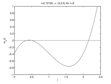
Figure 9. The graph of $H_{2}(l)$ in (3.8) (for $n=2$): $l=2.15159...$ .

For $n=1.8$ (still non-oscillatory), the value of $l$ is explained in Figure 10, where

(3.10) $$n=1.8:\quad l=2.1128...\,,$$

also satisfying conditions in (3.6).

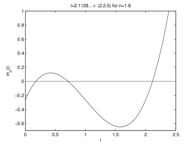
Figure 10. The graph of $H_{n}(l)$ in (3.8) for $n=1.8$: $l=2.1128...$ .

Finally, we have got that such a positive 1D bundle perfectly exists also in the oscillatory range, i.e., for $n<n_{\rm h}$: see Figure 11, where

(3.11) $$n=1.7<n_{\rm h}:\quad l=2.08074...\,.$$

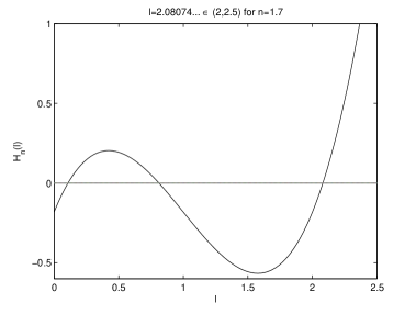
Figure 11. The graph of $H_{n}(l)$ in (3.8) for $n=1.7<n_{\rm h}$: $l=2.08074...$ .

Concerning a proper justification of the actual existence of the bundle (3.4), (3.8) on a small interval $y\in[0,\delta]$, on one hand, this can be done by reducing the third-order non-autonomous ODE (3.1) to a dynamical system in $\mathbb{R}^{4}$. On the other hand, since the right-hand side of

(3.12) $$\textstyle{f^{\prime\prime\prime}=-\frac{1-y}{f^{n-1}}}$$

is singular at $y=0$, there occurs an integrability problem. Indeed, a direct first integration of (3.12) over a small interval $(0,y)$ is impossible since, in the present parameter $n$-range, $f^{\prime\prime}(0)=+\infty$. Therefore, one has to use another representation of the equation.

To clarify this, consider, e.g., the case $n=2$. We then integrate (3.1) over $(0,y)$ to get

(3.13) $$\textstyle{ff^{\prime\prime}-\frac{1}{2}\,(f^{\prime})^{2}=-\big{(}y-\frac{y^{2}}{2}\big{)},}$$

where all accompanying integrals are convergent at $y=0$. Hence,

(3.14) $$\textstyle{f^{\prime\prime}=\frac{1}{f}\,\big{[}\frac{1}{2}\,(f^{\prime})^{2}-\big{(}y-\frac{y^{2}}{2}\big{)}\big{]}.}$$

Note that, in the class of solutions close to (3.4) (with $m=\frac{3}{2}$ for $n=2$), both terms on the right-hand side of (3.14) are equally involved into the behaviour of $f(y)$ as $y\to 0^{+}$. Integrating (3.14) two times, with all integrals convergent, since $m=\frac{3}{n}=\frac{3}{2}>1$, so $f^{\prime}(y)$ is locally bounded, we arrive at a system for $\{f,f^{\prime}\}$ of a standard form

(3.15) $$\left(\begin{matrix}f\\ f^{\prime}\end{matrix}\right)={\bf M}\left(\begin{matrix}f\\ f^{\prime}\end{matrix}\right),$$

with an integral operator ${\bf M}$, easily reconstructed from (3.14), being a contraction in $C([0,\delta])$ for sufficiently small $\delta>0$ (meaning $C^{1}$ for $f$) in a properly chosen invariant neighbourhood of each orbit from (3.4) for any fixed $D\in\mathbb{R}$. As a “measure” of this neighbourhood, one can use the third term in (3.4), i.e., that one appeared for $D=0$ (we have mentioned it above).

One can see from (3.8) that a proper characteristic root $l$ exists for all $n\in\big{(}\frac{3}{2},3\big{)}$, so that a positive expansion (3.4), (3.8) close to interfaces for the Cauchy problem always exists in this whole parameter range. Moreover, one can see that, in this parameter range,

(3.16) $$\textstyle{n\in\big{(}\frac{3}{2},3\big{)}:\quad f(0)=f^{\prime}(0)=(f^{n}f^{\prime\prime\prime})(0)=0,}$$

i.e., standard zero-high, zero-contact angle, and zero-flux conditions, which are requirements of the FBP (for the CP, exhibiting, usually, a smoother behaviour at the interface, those are also valid), take place.

We, thus, naturally, come to our:

4. Final conclusions

Thus, we have seen that the positive expansion (3.4), (3.8) exists for all $n$ in our range $n\in\big{(}\frac{3}{2},2]$, and also for all $n\in(2,3)$, though this range is out of our current interests.

So, the following natural question arises: why then do we need to take into account an oscillatory behaviour for $\frac{3}{2}<n<n_{\rm h}$? The answer is as follows:

1. It turns out that the shooting, via the positive 1D bundle (3.4), (3.8) posed at $y=y_{0}^{-}$, the single symmetry condition at the origin $f^{\prime}(0)=0$ is consistent not for all $n$’s, and only for $n\geq n_{\rm h}$.

2. So, there exists a heteroclinic bifurcation point $n=n_{\rm h}$, starting with which using positive expansion near the interface becomes inconsistent, so a new oscillatory 1D bundle is necessary, which allows to shoot a proper similarity profile $f(y)$.

A naive analogy in linear spectral non-self-adjoint theory is: a spectral parameter $\lambda$, starting at some critical value of a parameter, must become complex, with a non-zero imaginary part (meaning oscillations of eigenfunctions), in order to make consistent algebraic systems arising.

As a consequence and as an answer of a possible (quite reasonable) critics concerning a definite lack of rigorous results in the present paper on the actual global existence of the similarity profiles $f(y)$ for the Cauchy problem in our range $n\in(\frac{3}{2},2]$, it is worth mentioning that any kind of shooting using the positive or oscillatory bundle at the interface must reveal this critical exponent $n_{\rm h}$. Recall that $n$ comes from the ODE (2.2) by using a “microscopic blow-up” analysis of the ODE (1.5) for $f(y)$. We do not think that any king of a global-type study of this ODE (1.5) (without a blow-up one as $y\to y_{0}^{-}$) can reveal this critical heteroclinic exponent.

3. Finally, bearing in mind (3.16) and the uniqueness of an admissible (positive) expansion, we end up with the following expected conclusion:

(4.1) for $$n\in[n_{\rm h},3)$$, the FBP and CP have the same solutions,

which was already announced in our earlier papers, but, unfortunately, without sufficiently convincing details.

Acknowledgements. The author would like to thank J.D. Evans for discussions and good questions, essentially initiated the present research, to be continued for the sixth-order thing film equation (the TFE–6; in lines with our previous papers [14], where all asymptotic/numerical tools get more complicated).

References

- [1] J. Becker and G. Grün, The thin-film equation: recent advances and some new perspectives, J. Phys.: Condens. Matter, 17 (2005), S291–S307.
- [2] F. Bernis and A. Friedman, Higher order nonlinear degenerate parabolic equations, J. Differ. Equat., 83 (1990), 179–206.
- [3] F. Bernis, J. Hulshof, and J.R. King, Dipoles and similarity solutions of the thin film equation in the half-line, Nonlinearity, 13 (2000), 413–439.
- [4] F. Bernis, J. Hulshof, and F. Quirós, The “linear” limit of thin film flows as an obstacle-type free boundary problem, SIAM J. Appl. Math., 61 (2000), 1062–1079.
- [5] F. Bernis and J.B. McLeod, Similarity solutions of a higher order nonlinear diffusion equation, Nonl. Anal., 17 (1991), 1039–1068.
- [6] F. Bernis, L.A. Peletier, and S.M. Williams, Source type solutions of a fourth order nonlinear degenerate parabolic equation, Nonl. Anal., 18 (1992), 217–234.
- [7] M. Bowen, J. Hulshof, and J.R. King, Anomaluous exponents and dipole solutions for the thin film equation, SIAM J. Appl. Math., 62 (2001), 149–179.
- [8] M. Bowen and T.P. Witelski, The linear limit of the dipole problem for the thin film equation, SIAM J. Appl. Math., 66 (2006), 1727–1748.
- [9] E.C. Carlen and S. Ulusoy, Asymptotic equipartition and long-time behaviour of solutions of a thin film eqwuation, J. Differ. Equat., 241 (2007), 279–292.
- [10] J.A. Carrillo and G. Toscani, Long-time asymptotic behaviour for strong solutions of the thin film eqwuations, Comm. Math. Phys., 225 (2002), 551–571.
- [11] C.M. Elliott and H. Garcke, On the Cahn–Hilliard equation with degenerate mobility, SIAM J. Math. Anal., 27 (1996), 404–423.
- [12] C. Elliott and Z. Songmu, On the Cahn-Hilliard equation, Arch. Rat. Mech. Anal., 96 (1986), 339–357.
- [13] J.D. Evans, V.A. Galaktionov, and J.R. King, Source-type solutions of the fourth-order unstable thin film equation, Euro J. Appl. Math., 18 (2007), 273–321.
- [14] J.D. Evans, V.A. Galaktionov, and J.R. King, Unstable sixth-order thin film equation. I. Blow-up similarity solutions; II. Global similarity patterns, Nonlinearity, 20 (2007), 1799–1841, 1843–1881.
- [15] R. Ferreira and F. Bernis, Source-type solutions to thin-film equations in higher dimensions, European J. Appl. Math., 8 (1997), 507–524.
- [16] V.A. Galaktionov and P.J. Harwin, On centre subspace behaviour in thin film equations, SIAM J. Appl. Math., 69 (2009), 1334–1358 (an earlier preprint in arXiv:0901.3995).
- [17] V.A. Galaktionov and S.R. Svirshchevskii, Exact Solutions and Invariant Subspaces of Nonlinear Partial Differential Equations in Mechanics and Physics, ChapmanHall/CRC, Taylor and Francis Group, Boca Raton, FL, 2007.
- [18] L. Giacomelli, H. Knüpfer, and F. Otto, Smooth zero-contact-angle solutions to a thin film equation around the steady state, J. Differ. Equat., 245 (2008), 1454–1506.
- [19] H.P. Greenspan, On the motion of a small viscous droplet that wets a surface, J. Fluid Mech., 84 (1978), 125–143.
- [20] L.V. Govor, J. Parisi, G.H. Bauer, and G. Reiter, Instability and droplet formation in evaporating thin films of a binary solution, Phys. Rev. E, 71, 051603 (2005).
- [21] G. Grün, Degenerate parabolic equations of fourth order and a plasticity model with non-local hardening, Z. Anal. Anwendungen, 14 (1995), 541–573.
- [22] R.S. Laugesen and M.C. Pugh, Energy levels of steady states for thin-film-type equations, J. Differ. Equat., 182 (2002), 377–415.
- [23] A. Oron, S.H. Davies, and S.G. Bankoff, Long-scale evolution of thin liquids films, Rev. Modern Phys., 69 (1997), 931–980.
- [24] L. Perko, Differential Equations and Dynamical Systems, Springer-Verlag, New York, 1991.
- [25] N.F. Smyth and J.M. Hill, High-order nonlinear diffusion, IMA J. Appl. Math., 40 (1988), 73–86.
- [26] T.P. Witelski, A.J. Bernoff, and A.L. Bertozzi, Blow-up and dissipation in a critical-case unstable thin film equation, Euro J. Appl. Math., 15 (2004), 223–256.