Stochastic approximation of score functions for Gaussian processes

Abstract

We discuss the statistical properties of a recently introduced unbiased stochastic approximation to the score equations for maximum likelihood calculation for Gaussian processes. Under certain conditions, including bounded condition number of the covariance matrix, the approach achieves $O(n)$ storage and nearly $O(n)$ computational effort per optimization step, where $n$ is the number of data sites. Here, we prove that if the condition number of the covariance matrix is bounded, then the approximate score equations are nearly optimal in a well-defined sense. Therefore, not only is the approximation efficient to compute, but it also has comparable statistical properties to the exact maximum likelihood estimates. We discuss a modification of the stochastic approximation in which design elements of the stochastic terms mimic patterns from a $2^{n}$ factorial design. We prove these designs are always at least as good as the unstructured design, and we demonstrate through simulation that they can produce a substantial improvement over random designs. Our findings are validated by numerical experiments on simulated data sets of up to 1 million observations. We apply the approach to fit a space–time model to over 80,000 observations of total column ozone contained in the latitude band $40^{\circ}$–$50^{\circ}$N during April 2012.

T0Government License. The submitted manuscript has been created by UChicago Argonne, LLC, Operator of Argonne National Laboratory (“Argonne”). Argonne, a U.S. Department of Energy Office of Science laboratory, is operated under Contract No. DE-AC02-06CH11357. The U.S. Government retains for itself, and others acting on its behalf, a paid-up nonexclusive, irrevocable worldwide license in said article to reproduce, prepare derivative works, distribute copies to the public, and perform publicly and display publicly, by or on behalf of the Government.

, and

t1Supported by the U.S. Department of Energy Grant DE-SC0002557.

t2Supported by the U.S. Department of Energy through Contract DE-AC02-06CH11357.

1 Introduction

Gaussian process models are widely used in spatial statistics and machine learning. In most applications, the covariance structure of the process is at least partially unknown and must be estimated from the available data. Likelihood-based methods, including Bayesian methods, are natural choices for carrying out the inferences on the unknown covariance structure. For large data sets, however, calculating the likelihood function exactly may be difficult or impossible in many cases.

Assuming we are willing to specify the covariance structure up to some parameter $\theta\in\Theta\subset{\mathbb{R}}^{p}$, the generic problem we are faced with is computing the loglikelihood for $Z\sim N(0,K(\theta))$ for some random vector $Z\in{\mathbb{R}}^{n}$ and $K$ an $n\times n$ positive definite matrix indexed by the unknown $\theta$. In many applications, there would be a mean vector that also depends on unknown parameters, but since unknown mean parameters generally cause fewer computational difficulties, for simplicity we will assume the mean is known to be 0 throughout this work. For the application to ozone data in Section 6, we avoid modeling the mean by removing the monthly mean for each pixel. The simulations in Section 5 all first preprocess the data by taking a discrete Laplacian, which filters out any mean function that is linear in the coordinates, so that the results in those sections would be unchanged for such mean functions. The loglikelihood is then, up to an additive constant, given by

$${\cal L}(\theta)=-\tfrac{1}{2}Z^{\prime}K(\theta)^{-1}Z-\tfrac{1}{2}\log\det\bigl{\{}K(\theta)\bigr{\}}.$$

If $K$ has no exploitable structure, the standard direct way of calculating ${\cal L}(\theta)$ is to compute the Cholesky decompositon of $K(\theta)$, which then allows $Z^{\prime}K(\theta)^{-1}Z$ and $\log\det\{K(\theta)\}$ to be computed quickly. However, the Cholesky decomposition generally requires $O(n^{2})$ storage and $O(n^{3})$ computations, either of which can be prohibitive for sufficiently large $n$.

Therefore, it is worthwhile to develop methods that do not require the calculation of the Cholesky decomposition or other matrix decompositions of $K$. If our goal is just to find the maximum likelihood estimate (MLE) and the corresponding Fisher information matrix, we may be able to avoid the computation of the log determinants by considering the score equations, which are obtained by setting the gradient of the loglikelihood equal to 0. Specifically, defining $K_{i}=\frac{\partial}{\partial\theta_{i}}K(\theta)$, the score equations for $\theta$ are given by (suppressing the dependence of $K$ on $\theta$)

$$\tfrac{1}{2}Z^{\prime}K^{-1}K_{i}K^{-1}Z-\tfrac{1}{2}\operatorname{tr}\bigl{(}K^{-1}K_{i}\bigr{)}=0$$ (1)

for $i=1,\ldots,p$. If these equations have a unique solution for $\theta\in\Theta$, this solution will generally be the MLE.

Iterative methods often provide an efficient (in terms of both storage and computation) way of computing solves in $K$ (expressions of the form $K^{-1}x$ for vectors $x$) and are based on being able to multiply arbitrary vectors by $K$ rapidly. In particular, assuming the elements of $K$ can be calculated as needed, iterative methods require only $O(n)$ storage, unlike matrix decompositions such as the Cholesky, which generally require $O(n^{2})$ storage. In terms of computations, two factors drive the speed of iterative methods: the speed of matrix–vector multiplications and the number of iterations. Exact matrix–vector multiplication generally requires $O(n^{2})$ operations, but if the data form a partial grid, then it can be done in $O(n\log n)$ operations using circulant embedding and the fast Fourier transform. For irregular observations, fast multipole approximations can be used [Anitescu, Chen and Wang (2012)]. The number of iterations required is related to the condition number of $K$ (the ratio of the largest to smallest singular value), so that preconditioning [Chen (2005)] is often essential; see Stein, Chen and Anitescu (2012) for some circumstances under which one can prove that preconditioning works well.

Computing the first term in (1) requires only one solve in $K$, but the trace term requires $n$ solves (one for each column of $K_{i}$) for $i=1,\ldots,p$, which may be prohibitive in some circumstances. Recently, Anitescu, Chen and Wang (2012) analyzed and demonstrated a stochastic approximation of the trace term based on the Hutchinson trace estimator [Hutchinson (1990)]. To define it, let $U_{1},\ldots,U_{N}$ be i.i.d. random vectors in ${\mathbb{R}}^{n}$ with i.i.d. symmetric Bernoulli components, that is, taking on values 1 and $-1$ each with probability $\frac{1}{2}$. Define a set of estimating equations for $\theta$ by

$$g_{i}(\theta,N)=\frac{1}{2}Z^{\prime}K^{-1}K_{i}K^{-1}Z-\frac{1}{2N}\sum_{j=1}^{N}U_{j}^{\prime}K^{-1}K_{i}U_{j}=0$$ (2)

for $i=1,\ldots,p$. Throughout this work, $E_{\theta}$ means to take expectations over $Z\sim N(0,K(\theta))$ and over the $U_{j}$’s as well. Since $E_{\theta}(U_{1}^{\prime}K^{-1}K_{i}U_{1})=\operatorname{tr}(K^{-1}K_{i})$, $E_{\theta}g_{i}(\theta,N)=0$ and (2) provides a set of unbiased estimating equations for $\theta$. Therefore, we may hope that a solution to (2) will provide a good approximation to the MLE. The unbiasedness of the estimating equations (2) requires only that the components of the $U_{j}$’s have mean 0 and variance 1; but, subject to this constraint, Hutchinson (1990) shows that, assuming the components of the $U_{j}$’s are independent, taking them to be symmetric Bernoulli minimizes the variance of $U_{1}^{\prime}MU_{1}$ for any $n\times n$ matrix $M$. The Hutchinson trace estimator has also been used to approximate the GCV (generalized cross-validation) statistic in nonparametric regression [Girard (1998), Zhang et al. (2004)]. In particular, Girard (1998) shows that $N$ does not need to be large to obtain a randomized GCV that yields results nearly identical to those obtained using exact GCV.

Suppose for now that it is possible to take $N$ much smaller than $n$ and obtain an estimate of $\theta$ that is nearly as efficient statistically as the exact MLE. From here on, assume that any solves in $K$ will be done using iterative methods. In this case, the computational effort to computing (1) or (2) is roughly linear in the number of solves required (although see Section 4 for methods that make $N$ solves for a common matrix $K$ somewhat less than $N$ times the effort of one solve), so that (2) is much easier to compute than (1) when $N/n$ is small. An attractive feature of the approximation (2) is that if at any point one wants to obtain a better approximation to the score function, it suffices to consider additional $U_{j}$’s in (2). However, how exactly to do this if using the dependent sampling scheme for the $U_{j}$’s in Section 4 is not so obvious.

Since this stochastic approach provides only an approximation to the MLE, one must compare it with other possible approximations to the MLE. Many such approaches exist, including spectral methods, low-rank approximations, covariance tapering and those based on some form of composite likelihood. All these methods involve computing the likelihood itself and not just its gradient, and thus all share this advantage over solving (2). Note that one can use randomized algorithms to approximate $\log\det K$ and thus approximate the loglikelihood directly [Zhang (2006)]. However, this approximation requires first taking a power series expansion of $K$ and then applying the randomization trick to each term in the truncated power series; the examples presented by Zhang (2006) show that the approach does not generally provide a good approximation to the loglikelihood. Since the accuracy of the power series approximation to $\log\det K$ depends on the condition number of $K$, some of the filtering ideas described by Stein, Chen and Anitescu (2012) and used to good effect in Section 4 here could perhaps be of value for approximating $\log\det K$, but we do not explore that possibility. See Aune, Simpson and Eidsvik (2013) for some recent developments on stochastic approximation of log determinants of positive definite matrices.

Let us consider the four approaches of spectral methods, low-rank approximations, covariance tapering and composite likelihood in turn. Spectral approximations to the likelihood can be fast and accurate for gridded data [Whittle (1954), Guyon (1982), Dahlhaus and Künsch (1987)], although even for gridded data they may require some prefiltering to work well [Stein (1995)]. In addition, the approximations tend to work less well as the number of dimensions increase [Dahlhaus and Künsch (1987)] and thus may be problematic for space–time data, especially if the number of spatial dimensions is three. Spectral approximations have been proposed for ungridded data [Fuentes (2007)], but they do not work as well as they do for gridded data from either a statistical or computational perspective, especially if large subsets of observations do not form a regular grid. Furthermore, in contrast to the approach we propose here, there appears to be no easy way of improving the approximations by doing further calculations, nor is it clear how to assess the loss of efficiency by using spectral approximations without a large extra computational burden.

Low-rank approximations, in which the covariance matrix is approximated by a low-rank matrix plus a diagonal matrix, can greatly reduce the burden of memory and computation relative to the exact likelihood [Cressie and Johannesson (2008), Eidsvik et al. (2012)]. However, for the kinds of applications we have in mind, in which the diagonal component of the covariance matrix does not dominate the small-scale variation of the process, these low-rank approximations tend to work poorly and are not a viable option [Stein (2008)].

Covariance tapering replaces the covariance matrix of interest by a sparse covariance matrix with similar local behavior [Furrer, Genton and Nychka (2006)]. There is theoretical support for this approach [Kaufman, Schervish and Nychka (2008), Wang and Loh (2011)], but the tapered covariance matrix must be very sparse to help a great deal with calculating the log determinant of the covariance matrix, in which case Stein (2012) finds that composite likelihood approaches will often be preferable. There is scope for combining covariance tapering with the approach presented here in that sparse matrices lead to efficient matrix–vector multiplication, which is also essential for our implementation of computing (2) based on iterative methods to do the matrix solves. Sang and Huang (2012) show that covariance tapering and low-rank approximations can also sometimes be profitably combined to approximate likelihoods.

We consider methods based on composite likelihoods to be the main competitor to solving (2). The approximate loglikelihoods described by Vecchia (1988), Stein, Chi and Welty (2004), Caragea and Smith (2007) can all be written in the following form: for some sequence of pairs of matrices $(A_{j},B_{j})$, $j=1,\ldots,q$, all with $n$ columns, at most $n$ rows and full rank,

$$\sum_{j=1}^{q}\log f_{j,\theta}(A_{j}Z\mid B_{j}Z),$$ (3)

where $f_{j,\theta}$ is the conditional Gaussian density of $A_{j}Z$ given $B_{j}Z$. As proposed by Vecchia (1988) and Stein, Chi and Welty (2004), the rank of $B_{j}$ will generally be larger than that of $A_{j}$, in which case the main computation in obtaining (3) is finding Cholesky decompositions of the covariance matrices of $B_{1}Z,\ldots,B_{q}Z$. For example, Vecchia (1988) just lets $A_{j}Z$ be the $j$th component of $Z$ and $B_{j}Z$ some subset of $Z_{1},\ldots,Z_{j-1}$. If $m$ is the largest of these subsets, then the storage requirements for this computation are $O(m^{2})$ rather than $O(n^{2})$. Comparable to increasing the number of $U_{j}$’s in the randomized algorithm used here, this approach can be updated to obtain a better approximation of the likelihood by increasing the size of the subset of $Z_{1},\ldots,Z_{j-1}$ to condition on when computing the conditional density of $Z_{j}$. However, for this approach to be efficient from the perspective of flops, one needs to store the Cholesky decompositions of the covariance matrices of $B_{1}Z,\ldots,B_{q}Z$, which would greatly increase the memory requirements of the algorithm. For dealing with truly massive data sets, our long-term plan is to combine the randomized approach studied here with a composite likelihood by using the randomized algorithms to compute the gradient of (3), thus making it possible to consider $A_{j}$’s and $B_{j}$’s of larger rank than would be feasible if one had to do exact calculations.

Section 2 provides a bound on the efficiency of the estimating equations based on the approximate likelihood relative to the Fisher information matrix. The bound is in terms of the condition number of the true covariance matrix of the observations and shows that if the covariance matrix is well conditioned, $N$ does not need to be very large to obtain nearly optimal estimating equations. Section 3 shows how one can get improved estimating equations by choosing the $U_{j}$’s in (2) based on a design related to $2^{n}$ factorial designs. Section 4 describes details of the algorithms, including methods for solving the approximate score equations and the role of preconditioning. Section 5 provides results of numerical experiments on simulated data. These results show that the basic method can work well for moderate values of $N$, even sometimes when the condition numbers of the covariance matrices do not stay bounded as the number of observations increases. Furthermore, the algorithm with the $U_{j}$’s chosen as in Section 3 can lead to substantially more accurate approximations for a given $N$. A large-scale numerical experiment shows that for observations on a partially occluded grid, the algorithm scales nearly linearly in the sample size. Section 6 applies the methods to OMI (Ozone Monitoring Instrument) Level 3 (gridded) total column ozone measurements for April 2012 in the latitude band $40^{\circ}$–$50^{\circ}$N.

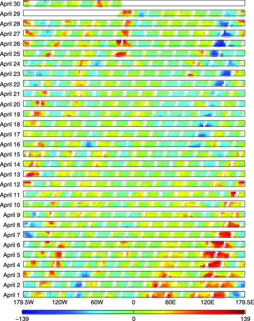
Figure 1: Demeaned ozone data (Dobson units) plotted using a heat color map. Missing data is colored white.

The data are given on a $1^{\circ}\times 1^{\circ}$ grid, so if the data were complete, there would be a total of $360\times 10\times 30=108\mbox{,}000$ observations. However, as Figure 1 shows, there are missing observations, mostly due to a lack of overlap in data from different orbits taken by OMI, but also due to nearly a full day of missing data on April 29–30, so that there are 84,942 observations. By acting as if all observations are taken at noon local time and assuming the process is stationary in longitude and time, the covariance matrix for the observations can be embedded in a block circulant matrix, greatly reducing the computational effort needed for multiplying the covariance matrix by a vector. Using (2) and a factorized sparse inverse preconditioner [Kolotilina and Yeremin (1993)], we are able to compute an accurate approximation to the MLE for a simple model that captures some of the main features in the OMI data, including the obvious movement of ozone from day to day visible in Figure 1 that coincides with the prevailing westerly winds in this latitude band.

2 Variance of stochastic approximation of the score function

This section gives a bound relating the covariance matrices of the approximate and exact score functions. Let us first introduce some general notation for unbiased estimating equations. Suppose $\theta$ has $p$ components and $g(\theta)=(g_{1}(\theta),\ldots,g_{p}(\theta))^{\prime}=0$ is a set of unbiased estimating equations for $\theta$ so that $E_{\theta}g(\theta)=0$ for all $\theta$. Write $\dot{g}(\theta)$ for the $p\times p$ matrix whose $ij$th element is $\frac{\partial}{\partial\theta_{i}}g_{j}(\theta)$ and $\operatorname{cov}_{\theta}\{g(\theta)\}$ for the covariance matrix of $g(\theta)$. The Godambe information matrix [Varin, Reid and Firth (2011)],

$$\mathcal{E}\bigl{\{}g(\theta)\bigr{\}}=E_{\theta}\bigl{\{}\dot{g}(\theta)\bigr{\}}\bigl{[}\operatorname{cov}_{\theta}\bigl{\{}g(\theta)\bigr{\}}\bigr{]}^{-1}E_{\theta}\bigl{\{}\dot{g}(\theta)\bigr{\}}$$

is a natural measure of the informativeness of the estimating equations [Heyde (1997), Definition 2.1]. For positive semidefinite matrices $A$ and $B$, write $A\succeq B$ if $A-B$ is positive semidefinite. For unbiased estimating equations $g(\theta)=0$ and $h(\theta)=0$, then we can say $g$ dominates $h$ if $\mathcal{E}\{g(\theta)\}\succeq\mathcal{E}\{h(\theta)\}$. Under sufficient regularity conditions on the model and the estimating equations, the score equations are the optimal estimating equations [Bhapkar (1972)]. Specifically, for the score equations, the Godambe information matrix equals the Fisher information matrix, ${\cal I}(\theta)$, so this optimality condition means ${\cal I}(\theta)\succeq\mathcal{E}\{g(\theta)\}$ for all unbiased estimating equations $g(\theta)=0$. Writing $M_{ij}$ for the $ij$th element of the matrix $M$, for the score equations in (1), ${\cal I}_{ij}(\theta)=\frac{1}{2}\operatorname{tr}(K^{-1}K_{i}K^{-1}K_{j})$ [Stein (1999), page 179]. For the approximate score equations (2), it is not difficult to show that $E_{\theta}\dot{g}(\theta,N)=-{\cal I}(\theta)$. Furthermore, writing $W^{i}$ for $K^{-1}K_{i}$ and defining the matrix ${\cal J}(\theta)$ by ${\cal J}_{ij}(\theta)=\operatorname{cov}(U_{1}^{\prime}W^{i}U_{1},U_{1}^{\prime}W^{j}U_{1})$, we have

$$\operatorname{cov}_{\theta}\bigl{\{}g(\theta,N)\bigr{\}}={\cal I}(\theta)+\frac{1}{4N}{\cal J}(\theta),$$ (4)

so that $\mathcal{E}\{g(\theta,N)\}={\cal I}(\theta)\{{\cal I}(\theta)+\frac{1}{4N}{\cal J}(\theta)\}^{-1}{\cal I}(\theta)$, which, as $N\to\infty$, tends to ${\cal I}(\theta)$.

In fact, as also demonstrated empirically by Anitescu, Chen and Wang (2012), one may often not need $N$ to be that large to get estimating equations that are nearly as efficient as the exact score equations. Writing $U_{1j}$ for the $j$th component of $U_{1}$, we have

$${\cal J}_{ij}(\theta) = \sum_{k,\ell,p,q=1}^{n}\operatorname{cov}\bigl{(}W_{k\ell}^{i}U_{1k}U_{1\ell},W_{pq}^{j}U_{1p}U_{1q}\bigr{)}$$

$$= \sum_{k\neq\ell}\bigl{\{}\operatorname{cov}\bigl{(}W_{k\ell}^{i}U_{1k}U_{1\ell},W_{k\ell}^{j}U_{1k}U_{1\ell}\bigr{)}+\operatorname{cov}\bigl{(}W_{k\ell}^{i}U_{1k}U_{1\ell},W_{\ell k}^{j}U_{1k}U_{1\ell}\bigr{)}\bigr{\}}$$

$$= \sum_{k\neq\ell}\bigl{(}W_{k\ell}^{i}W_{k\ell}^{j}+W_{k\ell}^{i}W_{\ell k}^{j}\bigr{)}$$

$$= \operatorname{tr}\bigl{(}W^{i}W^{j}\bigr{)}+\operatorname{tr}\bigl{\{}W^{i}\bigl{(}W^{j}\bigr{)}^{\prime}\bigr{\}}-2\sum_{k=1}^{n}W_{kk}^{i}W_{kk}^{j}.$$

As noted by Hutchinson (1990), the terms with $k=\ell$ drop out in the second step because $U_{1j}^{2}=1$ with probability 1. When $K(\theta)$ is diagonal for all $\theta$, then $N=1$ gives the exact score equations, although in this case computing $\operatorname{tr}(K^{-1}K_{i})$ directly would be trivial.

Writing $\kappa(\cdot)$ for the condition number of a matrix, we can bound$\operatorname{cov}_{\theta}\{g(\theta,N)\}$ in terms of ${\cal I}(\theta)$ and $\kappa(K)$. The proof of the following result is given in the Appendix.

Theorem 2.1

$$\operatorname{cov}_{\theta}\bigl{\{}g(\theta,N)\bigr{\}}\preceq{\cal I}(\theta)\biggl{\{}1+\frac{(\kappa(K)+1)^{2}}{4N\kappa(K)}\biggr{\}}.$$ (6)

It follows from (6) that

$$\mathcal{E}\bigl{\{}g(\theta,N)\bigr{\}}\succeq\biggl{\{}1+\frac{(\kappa(K)+1)^{2}}{4N\kappa(K)}\biggr{\}}^{-1}{\cal I}(\theta).$$

In practice, if $\frac{(\kappa(K)+1)^{2}}{4N\kappa(K)}<0.01$, so that the loss of information in using (2) rather than (1) was at most 1%, we would generally be satisfied with using the approximate score equations and a loss of information of even 10% or larger might be acceptable when one has a massive amount of data. For example, if $\kappa(K)=5$, a bound of 0.01 is obtained with $N=180$ and a bound of 0.1 with $N=18$.

It is possible to obtain unbiased estimating equations similar to (2) whose statistical efficiency does not depend on $\kappa(K)$. Specifically, if we write $\operatorname{tr}(K^{-1}K_{i})$ as $\operatorname{tr}((G^{\prime})^{-1}K_{i}G^{-1})$, where $G$ is any matrix satisfying $G^{\prime}G=K$, we then have that

$$h_{i}(\theta,N)=\frac{1}{2}Z^{\prime}K^{-1}K_{i}K^{-1}Z-\frac{1}{2N}\sum_{j=1}^{N}U_{j}^{\prime}\bigl{(}G^{\prime}\bigr{)}^{-1}K_{i}G^{-1}U_{j}=0$$ (7)

for $i=1,\ldots,p$ are also unbiased estimating equations for $\theta$. In this case, $\operatorname{cov}_{\theta}\{h(\theta,N)\}\preceq(1+\frac{1}{N}){\cal I}(\theta)$, whose proof is similar to that of Theorem 2.1 but exploits the symmetry of $(G^{\prime})^{-1}K_{i}G^{-1}$. This bound is less than or equal to the bound in (6) on $\operatorname{cov}_{\theta}\{g(\theta,N)\}$. Whether it is preferable to use (7) rather than (2) depends on a number of factors, including the sharpness of the bound in (6) and how much more work it takes to compute $G^{-1}U_{j}$ than to compute $K^{-1}U_{j}$. An example of how the action of such a matrix square root can be approximated efficiently using only $O(n)$ storage is presented by Chen, Anitescu and Saad (2011).

3 Dependent designs

Choosing the $U_{j}$’s independently is simple and convenient, but one can reduce the variation in the stochastic approximation by using a more sophisticated design for the $U_{j}$’s; this section describes such a design. Suppose that $n=Nm$ for some nonnegative integer $m$ and that $\beta_{1},\ldots,\beta_{N}$ are fixed vectors of length $N$ with all entries $\pm 1$ for which $\frac{1}{N}\sum_{j=1}^{N}\beta_{j}\beta^{\prime}_{j}=I$. For example, if $N=2^{q}$ for a positive integer $q$, then the $\beta_{j}$’s can be chosen to be the design matrix for a saturated model of a $2^{q}$ factorial design in which the levels of the factors are set at $\pm 1$ [Box, Hunter and Hunter (2005), Chapter 5]. In addition, assume that $X_{1},\ldots,X_{m}$ are random diagonal matrices of size $N$ and $Y_{jk}$, $j=1,\ldots,N;k=1,\ldots,m$ are random variables such that all the diagonal elements of the $X_{j}$’s and all the $Y_{jk}$’s are i.i.d. symmetric Bernoulli random variables. Then define

$$U_{j}=\pmatrix{Y_{j1}X_{1}\cr\vdots\cr Y_{jm}X_{m}}\beta_{j}.$$ (8)

One can easily show that for any $Nm\times Nm$ matrix $M$, $E(\frac{1}{N}\sum_{j=1}^{N}U_{j}^{\prime}MU_{j})=\operatorname{tr}(M)$. Thus, we can use this definition of the $U_{j}$’s in (2), and the resulting estimating equations are still unbiased.

This design is closely related to a class of designs introduced by Avron and Toledo (2011), who propose selecting the $U_{j}$’s as follows. Suppose $H$ is a Hadamard matrix, that is, an $n\times n$ orthogonal matrix with elements $\pm 1$. Avron and Toledo (2011) actually consider $H$ a multiple of a unitary matrix, but the special case $H$ Hadamard makes their proposal most similar to ours. Then, using simple random sampling (with replacement), they choose $N$ columns from this matrix and multiply this $n\times N$ matrix by an $n\times n$ diagonal matrix with diagonal entries made up of independent symmetric Bernoulli random variables. The columns of this resulting matrix are the $U_{j}$’s. We are also multiplying a subset of the columns of a Hadamard matrix by a random diagonal matrix, but we do not select the columns by simple random sampling from some arbitrary Hadamard matrix.

The extra structure we impose yields beneficial results in terms of the variance of the randomized trace approximation, as the following calculations show. Partitioning $M$ into an $m\times m$ array of $N\times N$ matrices with $k\ell$th block $M^{b}_{k\ell}$, we obtain the following:

$$\frac{1}{N}\sum_{j=1}^{N}U_{j}^{\prime}MU_{j}=\frac{1}{N}\sum_{k,\ell=1}^{m}\sum_{j=1}^{N}Y_{jk}Y_{j\ell}\beta_{j}^{\prime}X_{k}M^{b}_{k\ell}X_{\ell}\beta_{j}.$$ (9)

Using $Y_{jk}^{2}=1$ and $X_{k}^{2}=I$, we have

$$\frac{1}{N}\sum_{j=1}^{N}Y_{jk}^{2}\beta_{j}^{\prime}X_{k}M^{b}_{kk}X_{k}\beta_{j} = \frac{1}{N}\operatorname{tr}\Biggl{(}X_{k}M^{b}_{kk}X_{k}\sum_{j=1}^{N}\beta_{j}\beta_{j}^{\prime}\Biggr{)}$$

$$= \operatorname{tr}\bigl{(}M^{b}_{kk}X_{k}^{2}\bigr{)}$$

$$= \operatorname{tr}\bigl{(}M^{b}_{kk}\bigr{)},$$

which is not random. Thus, if $M$ is block diagonal (i.e., $M^{b}_{k\ell}$ is a matrix of zeroes for all $k\neq\ell$), (9) yields $\operatorname{tr}(M)$ without error. This result is an extension of the result that independent $U_{j}$’s give $\operatorname{tr}(M)$ exactly for diagonal $M$. Furthermore, it turns out that, at least in terms of the variance of $\frac{1}{N}\sum_{j=1}^{N}U_{j}^{\prime}MU_{j}$, for the elements of $M$ off the block diagonal, we do exactly the same as we do when the $U_{j}$’s are independent. Write $B(\theta)$ for $\operatorname{cov}\{g(\theta,N)\}$ with $g(\theta,N)$ defined as in (2) with independent $U_{j}$’s. Define $g^{d}(\theta,N)=0$ for the unbiased estimating equations defined by (2) with dependent $U_{j}$’s defined by (8) and $B^{d}(\theta)$ to be the covariance matrix of $g^{d}(\theta,N)$. Take $T(N,n)$ to be the set of pairs of positive integers $(k,\ell)$ with $1\leq\ell<k\leq n$ for which $\lfloor k/N\rfloor=\lfloor\ell/N\rfloor$. We have the following result, whose proof is given in the Appendix.

Theorem 3.1

For any vector $v=(v_{1},\ldots,v_{p})^{\prime}$,

$$v^{\prime}B(\theta)v-v^{\prime}B^{d}(\theta)v=\frac{2}{N}\sum_{(k,\ell)\in T(N,n)}\Biggl{\{}\sum_{i=1}^{p}v_{i}\bigl{(}W_{k\ell}^{i}+W_{\ell k}^{i}\bigr{)}\Biggr{\}}^{2}.$$ (10)

Thus, $B(\theta)\succeq B^{d}(\theta)$. Since $E_{\theta}\dot{g}(\theta,N)=E_{\theta}\dot{g}^{d}(\theta,N)=-\mathcal{I}(\theta)$, it follows that $\mathcal{E}\{g^{d}(\theta,N)\}\succeq\mathcal{E}\{g(\theta,N)\}$.

How much of an improvement will result from using dependent $U_{j}$’s depends on the size of the $W_{k\ell}^{i}$’s within each block. For spatial data, one would typically group spatially contiguous observations within blocks. How to block for space–time data is less clear. The results here focus on the variance of the randomized trace approximation. Avron and Toledo (2011) obtain bounds on the probability that the approximation error is less than some quantity and note that these results sometimes give rankings for various randomized trace approximations different from those obtained by comparing variances.

4 Computational aspects

Finding $\theta$ that solves the estimating equations (2) requires a nonlinear equation solver in addition to computing linear solves in $K$. The nonlinear solver starts at an initial guess $\theta^{0}$ and iteratively updates it to approach a (hopefully unique) zero of (2). In each iteration, at $\theta^{i}$, the nonlinear solver typically requires an evaluation of $g(\theta^{i},N)$ in order to find the next iterate $\theta^{i+1}$. In turn, the evaluation of $g$ requires employing a linear solver to compute the set of vectors $K^{-1}Z$ and $K^{-1}U_{j}$, $j=1,\ldots,N$.

The Fisher information matrix $\mathcal{I}(\theta)$ and the matrix $\mathcal{J}(\theta)$ contain terms involving matrix traces and diagonals. Write $\operatorname{diag}(\cdot)$ for a column vector containing the diagonal elements of a matrix and $\circ$ for the Hadamard (elementwise) product of matrices. For any real matrix $A$,

$$\operatorname{tr}(A)=E_{U}\bigl{(}U^{\prime}AU\bigr{)}\quad\mbox{and}\quad\operatorname{diag}(A)=E_{U}(U\circ AU),$$

where the expectation $E_{U}$ is taken over $U$, a random vector with i.i.d. symmetric Bernoulli components. One can unbiasedly estimate $\mathcal{I}(\theta)$ and $\mathcal{J}(\theta)$ by

$$\widehat{\mathcal{I}}_{ij}(\theta)=\frac{1}{2N_{2}}\sum_{k=1}^{N_{2}}U_{k}^{\prime}W^{i}W^{j}U_{k}$$ (11)

and

$$\widehat{\mathcal{J}}_{ij}(\theta) = \frac{1}{N_{2}}\sum_{k=1}^{N_{2}}U_{k}^{\prime}W^{i}W^{j}U_{k}+\frac{1}{N_{2}}\sum_{k=1}^{N_{2}}U_{k}^{\prime}W^{i}\bigl{(}W^{j}\bigr{)}^{\prime}U_{k}$$

$${}-2\sum_{\ell=1}^{n}\Biggl{[}\frac{1}{N_{2}}\sum_{k=1}^{N_{2}}\bigl{(}U_{k}\circ W^{i}U_{k}\bigr{)}\Biggr{]}_{\ell}\Biggl{[}\frac{1}{N_{2}}\sum_{k=1}^{N_{2}}\bigl{(}U_{k}\circ W^{j}U_{k}\bigr{)}\Biggr{]}_{\ell}.$$

Note that here the set of vectors $U_{k}$ need not be the same as that in (2) and that $N_{2}$ may not be the same as $N$, the number of $U_{j}$’s used to compute the estimate of $\theta$. Evaluating $\widehat{\mathcal{I}}(\theta)$ and $\widehat{\mathcal{J}}(\theta)$ requires linear solves since $W^{i}U_{k}=K^{-1}(K_{i}U_{k})$ and $(W^{i})^{\prime}U_{k}=K_{i}(K^{-1}U_{k})$. Note that one can also unbiasedly estimate $\mathcal{J}_{ij}(\theta)$ as the sample covariance of $U^{\prime}_{k}W^{i}U_{k}$ and $U^{\prime}_{k}W^{j}W_{k}$ for $k=1,\ldots,N$, but (4) directly exploits properties of symmetric Bernoulli variables (e.g., $U^{2}_{1j}=1$). Further study would be needed to see when each approach is preferred.

4.1 Linear solver

We consider an iterative solver for solving a set of linear equations $Ax=b$ for a symmetric positive definite matrix $A\in{\mathbb{R}}^{n\times n}$, given a right-hand vector $b$. Since the matrix $A$ (in our case the covariance matrix) is symmetric positive definite, the conjugate gradient algorithm is naturally used. Let $x^{i}$ be the current approximate solution, and let $r^{i}=b-Ax^{i}$ be the residual. The algorithm finds a search direction $q^{i}$ and a step size $\alpha^{i}$ to update the approximate solution, that is, $x^{i+1}=x^{i}+\alpha^{i}q^{i}$, such that the search directions $q^{i},\ldots,q^{0}$ are mutually $A$-conjugate [i.e., $(q^{i})^{\prime}Aq^{j}=0$ for $i\neq j$] and the new residual $r^{i+1}$ is orthogonal to all the previous ones, $r^{i},\ldots,r^{0}$. One can show that the search direction is a linear combination of the current residual and the past search direction, yielding the following recurrence formulas:

$$x^{i+1} = x^{i}+\alpha^{i}q^{i},$$

$$r^{i+1} = r^{i}-\alpha^{i}Aq^{i},$$

$$q^{i+1} = r^{i+1}+\beta^{i}q^{i},$$

where $\alpha^{i}=\langle r^{i},r^{i}\rangle/\langle Aq^{i},q^{i}\rangle$ and $\beta^{i}=\langle r^{i+1},r^{i+1}\rangle/\langle r^{i},r^{i}\rangle$, and $\langle\cdot,\cdot\rangle$ denotes the vector inner product. Letting $x^{*}$ be the exact solution, that is, $Ax^{*}=b$, then $x^{i}$ enjoys a linear convergence to $x^{*}$:

$$\bigl{\|}x^{i}-x^{*}\bigr{\|}_{A}\leq 2\biggl{(}\frac{\sqrt{\kappa(A)}-1}{\sqrt{\kappa(A)}+1}\biggr{)}^{i}\bigl{\|}x^{0}-x^{*}\bigr{\|}_{A},$$ (13)

where $\|\cdot\|_{A}=\langle A\cdot,\cdot\rangle^{{1/2}}$ is the $A$-norm of a vector.

Asymptotically, the time cost of one iteration is upper bounded by that of multiplying $A$ by $q^{i}$, which typically dominates other vector operations when $A$ is not sparse. Properties of the covariance matrix can be exploited to efficiently compute the matrix–vector products. For example, when the observations are on a lattice (regular grid), one can use the fast Fourier transform (FFT), which takes time $O(n\log n)$ [Chan and Jin (2007)]. Even when the grid is partial (with occluded observations), this idea can still be applied. On the other hand, for nongridded observations, exact multiplication generally requires $O(n^{2})$ operations. However, one can use a combination of direct summations for close-by points and multipole expansions of the covariance kernel for faraway points to compute the matrix–vector products in $O(n\log n)$, even $O(n)$, time [Barnes and Hut (1986), Greengard and Rokhlin (1987)]. In the case of Matérn-type Gaussian processes and in the context of solving the stochastic approximation (2), such fast multipole approximations were presented by Anitescu, Chen and Wang (2012). Note that the total computational cost of the solver is the cost of each iteration times the number of iterations, the latter being usually much less than $n$.

The number of iterations to achieve a desired accuracy depends on how fast $x^{i}$ approaches $x^{*}$, which, from (13), is in turn affected by the condition number $\kappa$ of $A$. Two techniques can be used to improve convergence. One is to perform preconditioning in order to reduce $\kappa$; this technique will be discussed in the next section. The other is to adopt a block version of the conjugate gradient algorithm. This technique is useful for solving the linear system for the same matrix with multiple right-hand sides. Specifically, denote by $AX=B$ the linear system one wants to solve, where $B$ is a matrix with $s$ columns, and the same for the unknown $X$. Conventionally, matrices such as $B$ are called block vectors, honoring the fact that the columns of $B$ are handled simultaneously. The block conjugate gradient algorithm is similar to the single-vector version except that the iterates $x^{i}$, $r^{i}$ and $q^{i}$ now become block iterates $X^{i}$, $R^{i}$ and $Q^{i}$ and the coefficients $\alpha^{i}$ and $\beta^{i}$ become $s\times s$ matrices. The detailed algorithm is not shown here; interested readers are referred to O’Leary (1980). If $X^{*}$ is the exact solution, then $X^{i}$ approaches $X^{*}$ at least as fast as linearly:

$$\bigl{\|}\bigl{(}X^{i}\bigr{)}_{j}-\bigl{(}X^{*}\bigr{)}_{j}\bigr{\|}_{A}\leq C_{j}\biggl{(}\frac{\sqrt{\kappa_{s}(A)}-1}{\sqrt{\kappa_{s}(A)}+1}\biggr{)}^{i},\qquad j=1,\ldots,s,$$ (14)

where $(X^{i})_{j}$ and $(X^{*})_{j}$ are the $j$th column of $X^{i}$ and $X^{*}$, respectively; $C_{j}$ is some constant dependent on $j$ but not $i$; and $\kappa_{s}(A)$ is the ratio between $\lambda_{n}(A)$ and $\lambda_{s}(A)$ with the eigenvalues $\lambda_{k}$ sorted increasingly. Comparing (13) with (14), we see that the modified condition number $\kappa_{s}$ is less than $\kappa$, which means that the block version of the conjugate gradient algorithm has a faster convergence than the standard version does. In practice, since there are many right-hand sides (i.e., the vectors $Z$, $U_{j}$’s and $K_{i}U_{k}$’s), we always use the block version.

4.2 Preconditioning/filtering

Preconditioning is a technique for reducing the condition number of the matrix. Here, the benefit of preconditioning is twofold: it encourages the rapid convergence of an iterative linear solver and, if the effective condition number is small, it strongly bounds the uncertainty in using the estimating equations (2) instead of the exact score equations (1) for estimating parameters (see Theorem 2.1). In numerical linear algebra, preconditioning refers to applying a matrix $M$, which approximates the inverse of $A$ in some sense, to both sides of the linear system of equations. In the simple case of left preconditioning, this amounts to solving $MAx=Mb$ for $MA$ better conditioned than $A$. With certain algebraic manipulations, the matrix $M$ enters into the conjugate gradient algorithm in the form of multiplication with vectors. For the detailed algorithm, see Saad (2003). This technique does not explicitly compute the matrix $MA$, but it requires that the matrix–vector multiplications with $M$ can be efficiently carried out.

For covariance matrices, certain filtering operations are known to reduce the condition number, and some can even achieve an optimal preconditioning in the sense that the condition number is bounded by a constant independent of the size of the matrix [Stein, Chen and Anitescu (2012)]. Note that these filtering operations may or may not preserve the rank/size of the matrix. When the rank is reduced, then some loss of statistical information results when filtering, although similar filtering is also likely needed to apply spectral methods for strongly correlated spatial data on a grid [Stein (1995)]. Therefore, we consider applying the same filter to all the vectors and matrices in the estimating equations, in which case (2) becomes the stochastic approximation to the score equations of the filtered process. Evaluating the filtered version of $g(\theta,N)$ becomes easier because the linear solves with the filtered covariance matrix converge faster.

4.3 Nonlinear solver

The choice of the nonlinear solver is problem dependent. The purpose of solving the score equations (1) or the estimating equations (2) is to maximize the loglikelihood function $\mathcal{L}(\theta)$. Therefore, investigation into the shape of the loglikelihood surface helps identify an appropriate solver.

In Section 5, we consider the power law generalized covariance model ($\alpha>0$):

$$G(x;\theta)=\cases{\Gamma(-\alpha/2)r^{\alpha},&\quad if $\alpha/2\notin{\mathbb{N}}$,\cr(-1)^{1+\alpha/2}r^{\alpha}\log r,&\quad if $\alpha/2\in{\mathbb{N}}$,}$$ (15)

where $x=[x_{1},\ldots,x_{d}]\in{\mathbb{R}}^{d}$ denotes coordinates, $\theta$ is the set of parameters containing $\alpha>0$, $\ell=[\ell_{1},\ldots,\ell_{d}]\in{\mathbb{R}}^{d}$, and $r$ is the elliptical radius

$$r=\sqrt{\frac{x_{1}^{2}}{\ell_{1}^{2}}+\cdots+\frac{x_{d}^{2}}{\ell_{d}^{2}}}.$$ (16)

Allowing a different scaling in different directions may be appropriate when, for example, variations in a vertical direction may be different from those in a horizontal direction. The function $G$ is conditionally positive definite; therefore, only the covariances of authorized linear combinations of the process are defined [Chilès and Delfiner (2012), Section 4.3]. In fact, $G$ is $p$-conditionally positive definite if and only if $2p+2>\alpha$ [see Chilès and Delfiner (2012), Section 4.5], so that applying the discrete Laplace filter (which gives second-order differences) $\tau$ times to the observations yields a set of authorized linear combinations when $\tau\geq\frac{1}{2}\alpha$. Stein, Chen and Anitescu (2012) show that if $\alpha=4\tau-d$, then the covariance matrix has a bounded condition number independent of the matrix size. Consider the grid $\{\delta\mathbf{j}\}$ for some fixed spacing $\delta$ and $\mathbf{j}$ a vector whose components take integer values between $0$ and $m$. Applying the filter $\tau$ times, we obtain the covariance matrix

$$K_{\mathbf{i}\mathbf{j}}=\operatorname{cov}\bigl{\{}\Delta^{\tau}Z(\delta\mathbf{i}),\Delta^{\tau}Z(\delta\mathbf{j})\bigr{\}},$$

where $\Delta$ denotes the discrete Laplace operator

$$\Delta Z(\delta\mathbf{j})=\sum_{p=1}^{d}\bigl{\{}Z(\delta\mathbf{j}-\delta\mathbf{e}_{p})-2Z(\delta\mathbf{j})+Z(\delta\mathbf{j}+\delta\mathbf{e}_{p})\bigr{\}}$$

with $\mathbf{e}_{p}$ meaning the unit vector along the $p$th coordinate. If $\tau=\operatorname{round}((\alpha+d)/4)$, the resulting $K$ is both positive definite and reasonably well conditioned.

Figure 2 shows a sample loglikelihood surface for $d=1$ based on an observation vector $Z$ simulated from a 1D partial regular grid spanning the range $[0,100]$, using parameters $\alpha=1.5$ and $\ell=10$. (A similar 2D grid is shown later in Figure 3.) The peak of the surface is denoted by the solid white dot, which is not far away from the truth $\theta=(1.5,10)$. The white dashed curve (profile of the surface) indicates the maximum loglikelihoods $\mathcal{L}$ given $\alpha$. The curve is also projected on the $\alpha-\mathcal{L}$ plane and the $\alpha-\ell$ plane. One sees that the loglikelihood value has small variation (ranges from $48$ to $58$) along this curve compared with the rest of the surface, whereas, for example, varying just the parameter $\ell$ changes the loglikelihood substantially.

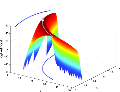
Figure 2: A sample loglikelihood surface for the power law generalized covariance kernel, with profile curve and peak plotted.

A Newton-type nonlinear solver starts at some initial point $\theta^{0}$ and tries to approach the optimal point (one that solves the score equations). Let the current point be $\theta^{i}$. The solver finds a direction $q^{i}$ and a step size $\alpha^{i}$ in some way to move the point to $\theta^{i+1}=\theta^{i}+\alpha^{i}q^{i}$, so that the value of $\mathcal{L}$ is increased. Typically, the search direction $q^{i}$ is the inverse of the Jacobian multiplied by $\theta^{i}$, that is, $q^{i}=\dot{g}(\theta^{i},N)^{-1}\theta^{i}$. This way, $\theta^{i+1}$ is closer to a solution of the score equations. Figure 2 shows a loglikelihood surface when $d=1$. The solver starts somewhere on the surface and quickly climbs to a point along the profile curve. However, this point might be far away from the peak. It turns out that along this curve a Newton-type solver is usually unable to find a direction with an appropriate step size to numerically increase $\mathcal{L}$, in part because of the narrow ridge indicated in the figure. The variation of $\mathcal{L}$ along the normal direction of the curve is much larger than that along the tangent direction. Thus, the iterate $\theta^{i}$ is trapped and cannot advance to the peak. In such a case, even though the estimated maximized likelihood could be fairly close to the true maximum, the estimated parameters could be quite distant from the MLE of $(\alpha,\ell)$.

To successfully solve the estimating equations, we consider each component of $\ell$ an implicit function of $\alpha$. Denote by

$$g_{i}(\alpha,\ell_{1},\ldots,\ell_{d})=0,\qquad i=1,\ldots,d+1,$$ (17)

the estimating equations, ignoring the fixed variable $N$. The implicit function theorem indicates that a set of functions $\ell_{1}(\alpha),\ldots,\ell_{d}(\alpha)$ exists around an isolated zero of (17) in a neighborhood where (17) is continuously differentiable, such that

$$g_{i}\bigl{(}\alpha,\ell_{1}(\alpha),\ldots,\ell_{d}(\alpha)\bigr{)}=0\qquad\mbox{for }i=2,\ldots,d+1.$$

Therefore, we need only to solve the equation

$$g_{1}\bigl{(}\alpha,\ell_{1}(\alpha),\ldots,\ell_{d}(\alpha)\bigr{)}=0$$ (18)

with a single variable $\alpha$. Numerically, a much more robust method than a Newton-type method exists for finding a root of a one-variable function. We use the standard method of Forsythe, Malcolm and Moler [(1976/1977), see the Fortran code Zeroin] for solving (18). This method in turn requires the evaluation of the left-hand side of (18). Then, the $\ell_{i}$’s are evaluated by solving $g_{2},\ldots,g_{d+1}=0$ fixing $\alpha$, whereby a Newton-type algorithm is empirically proven to be an efficient method.

5 Experiments

In this section we show a few experimental results based on a partially occluded regular grid. The rationale for using such a partial grid is to illustrate a setting where spectral techniques do not work so well but efficient matrix–vector multiplications are available. A partially occluded grid can occur, for example, when observations of some surface characteristics are taken by a satellite-based instrument and it is not possible to obtain observations over regions with sufficiently dense cloud cover. The ozone example in Section 6 provides another example in which data on a partial grid occurs. This section considers a grid with physical range $[0,100]\times[0,100]$ and a hole in a disc shape of radius $10$ centered at $(40,60)$. An illustration of the grid, with size $32\times 32$, is shown in Figure 3. The matrix–vector multiplication is performed by first doing the multiplication using the full grid via circulant embedding and FFT, followed by removing the entries corresponding to the hole of the grid. Recall that the covariance model is defined in Section 4.3, along with the explanation of the filtering step.

Figure 3: A $32\times 32$ grid with a region of missing observations in a disc shape. Internal grid points are grouped to work with the dependent design in Section 3.

When working with dependent samples, it is advantageous to group nearby grid points such that the resulting blocks have a plump shape and that there are as many blocks with size exactly $N$ as possible. For an occluded grid, this is a nontrivial task. Here we use a simple heuristic to effectively group the points. We divide the grid into horizontal stripes of width $\lfloor\sqrt{N}\rfloor$ (in case $\lfloor\sqrt{N}\rfloor$ does not divide the grid size along the vertical direction, some stripes have a width $\lfloor\sqrt{N}\rfloor+1$). The stripes are ordered from bottom to top, and the grid points inside the odd-numbered stripes are ordered lexicographically in their coordinates, that is, $(x,y)$. In order to obtain as many contiguous blocks as possible, the grid points inside the even-numbered stripes are ordered lexicographically according to $(-x,y)$. This ordering gives a zigzag flow of the points starting from the bottom-left corner of the grid. Every $N$ points are grouped in a block. The coloring of the grid points in Figure 3 shows an example of the grouping. Note that because of filtering, observations on either an external or internal boundary are not part of any block.

5.1 Choice of $N$

One of the most important factors that affect the efficacy of approximating the score equations is the value $N$. Theorem 2.1 indicates that $N$ should increase at least like $\kappa(K)$ in order to guarantee the additional uncertainty introduced by approximating the score equations be comparable with that caused by the randomness of the sample $Z$. In the ideal case, when the condition number of the matrix (possibly with filtering) is bounded independent of the matrix size $n$, then even taking $N=1$ is sufficient to obtain estimates with the same rate of convergence as the exact score equations. When $\kappa$ grows with $n$, however, a better guideline for selecting $N$ is to consider the growth of $\mathcal{I}^{-1}\mathcal{J}$.

Figure 4 plots the condition number of $K$ and the spectral norm of $\mathcal{I}^{-1}\mathcal{J}$ for varying sizes of the matrix and preconditioning using the Laplacian filter. Although performing a Laplacian filtering will yield provably bounded condition numbers only for the case $\alpha=2$, one sees that the filtering is also effective for the cases $\alpha=1$ and $1.5$. Moreover, the norm of $\mathcal{I}^{-1}\mathcal{J}$ is significantly smaller than $\kappa$ when $n$ is large and, in fact, it does not seem to grow with $n$. This result indicates the bound in Theorem 1 is sometimes far too conservative and that using a fixed $N$ can be effective even when $\kappa$ grows with $n$.

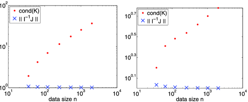
Figure 4: Growth of $\kappa$ compared with that of $\|\mathcal{I}^{-1}\mathcal{J}\|$, for power law kernel in 2D. Left: $\alpha=1$; right: $\alpha=1.5$.

Of course, the norm of $\mathcal{I}^{-1}\mathcal{J}$ is not always bounded. In Figure 5 we show two examples using the Matérn covariance kernel with smoothness parameter $\nu=1$ and 1.5 (essentially $\alpha=2$ and 3). Without filtering, both $\kappa(K)$ and $\|\mathcal{I}^{-1}\mathcal{J}\|$ grow with $n$, although the plots show that the growth of the latter is significantly slower than that of the former.

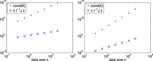
Figure 5: Growth of $\kappa$ compared with that of $\|\mathcal{I}^{-1}\mathcal{J}\|$, for Matérn kernel in 1D, without filtering. Left: $\nu=1$; right: $\nu=1.5$.

If the occluded observations are more scattered, then the fast matrix–vector multiplication based on circulant embedding still works fine. However, if the occluded pixels are randomly located and the fraction of occluded pixels is substantial, then using a filtered data set only including Laplacians centered at those observations whose four nearest neighbors are also available might lead to an unacceptable loss of information. In this case, one might instead use a preconditioner based on a sparse approximation to the inverse Cholesky decomposition as described in Section 6.

5.2 A $32\times 32$ grid example

Here, we show the details of solving the estimating equations (2) using a $32\times 32$ grid as an example. Setting the truth $\alpha=1.5$ and $\ell=(7,10)$ [i.e., $\theta=(1.5,7,10)$], consider exact and approximate maximum likelihood estimation based on the data obtained by applying the Laplacian filter once to the observations. Writing $\mathcal{G}$ for $\mathcal{E}\{g(\theta,N)\}$, one way to evaluate the approximate MLEs is to compute the ratios of the square roots of the diagonal elements of $\mathcal{G}^{-1}$ to the square roots of the diagonal elements of $\mathcal{I}^{-1}$. We know these ratios must be at least 1, and that the closer they are to 1, the more nearly optimal the resulting estimating equations based on the approximate score function are. For $N=64$ and independent sampling, we get 1.0156, 1.0125 and 1.0135 for the three ratios, all of which are very close to 1. Since one generally cannot calculate $\mathcal{G}^{-1}$ exactly, it is also worthwhile to compare a stochastic approximation of the diagonal values of $\mathcal{G}^{-1}$ to their exact values. When this approximation was done once for $N=64$ and by using $N_{2}=100$ in (11) and (4), the three ratios obtained were 0.9821, 0.9817 and 0.9833, which are all close to 1.

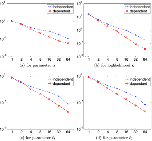
Figure 6: Effects of $N$ (1, 2, 4, 8, 16, 32, 64). In each plot, the curve with the plus sign corresponds to the independent design, whereas that with the circle sign corresponds to the dependent design. The horizontal axis represents $N$. In plots (a), (c) and (d), the vertical axis represents the mean squared differences between the approximate and exact MLEs divided by the mean squared errors for the exact MLEs, for the components $\alpha$, $\ell_{1}$ and $\ell_{2}$, respectively. In plot (b), the vertical axis represents the mean squared difference between the loglikelihood values at the exact and approximate MLEs.

Figure 6 shows the performance of the resulting estimates (to be compared with the exact MLEs obtained by solving the standard score equations). For $N=1$, $2$, $4$, $8$, $16$, $32$ and $64$, we simulated 100 realizations of the process on the $32\times 32$ occluded grid, applied the discrete Laplacian once, and then computed exact MLEs and approximations using both independent and dependent (as described in the beginning of Section 5) sampling. When $N=1$, the independent and dependent sampling schemes are identical, so only results for independent sampling are given. Figure 6 plots, for each component of $\theta$, the mean squared differences between the approximate and exact MLEs divided by the mean squared errors for the exact MLEs. As expected, these ratios decrease with $N$, particularly for dependent sampling. Indeed, dependent sampling is much more efficient than independent sampling for larger $N$; for example, the results in Figure 6 show that dependent sampling with $N=32$ yields better estimates for all three parameters than does independent sampling with $N=64$.

5.3 Large-scale experiments

We experimented with larger grids (in the same physical range). We show the results in Table 1 and Figure 7 for $N=64$. When the matrix becomes large, we are unable to compute $\mathcal{I}$ and $\mathcal{G}$ exactly. Based on the preceding experiment, it seems reasonable to use $N_{2}=100$ in approximating $\mathcal{I}$ and $\mathcal{G}$. Therefore, the elements of $\mathcal{I}$ and $\mathcal{G}$ in Table 1 were computed only approximately.

Table 1: Estimates and estimated standard errors for increasingly dense grids. The last three rows show the ratio of standard errors of the approximate to the exact MLEs

Grid size	$\bolds{32\times 32}$	$\bolds{64\times 64}$	$\bolds{128\times 128}$	$\bolds{256\times 256}$	$\bolds{512\times 512}$	$\bolds{1024\times 1024}$
$\widehat{\theta}^{N}$	1.5355	$1.5084$	$1.4919$	$1.4975$	1.5011	1.5012
	6.8507	$6.9974$	$7.1221$	$7.0663$	6.9841	6.9677
	9.2923	$10.062$	$10.091$	$10.063$	9.9818	9.9600
$\sqrt{(\mathcal{I}^{-1})_{ii}}$	0.0882	$0.0406$	$0.0196$	$0.0096$	0.0048	0.0024
	0.5406	$0.3673$	$0.2371$	$0.1464$	0.0877	0.0512
	0.8515	$0.5674$	$0.3605$	$0.2202$	0.1309	0.0760
$\frac{\sqrt{(\mathcal{G}^{-1})_{ii}}}{\sqrt{(\mathcal{I}^{-1})_{ii}}}$	1.0077	$1.0077$	$1.0077$	$1.0077$	1.0077	1.0077
	1.0062	$1.0070$	$1.0073$	$1.0074$	1.0075	1.0076
	1.0064	$1.0071$	$1.0073$	$1.0075$	1.0075	1.0076

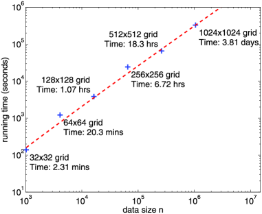
Figure 7: Running time for increasingly dense grids. The dashed curve fits the recorded times with a function of the form of $n\log n$ times a constant.

One sees that as the grid becomes larger (denser), the variance of the estimates decreases as expected. The matrices $\mathcal{I}^{-1}$ and $\mathcal{G}^{-1}$ are comparable in all cases and, in fact, the ratios stay roughly the same across different sizes of the data. The experiments were run for data size up to around one million, and the scaling of the running time versus data size is favorable. The results show a strong agreement of the recorded times with the scaling $O(n\log n)$.

6 Application

Ozone in the stratosphere blocks ultraviolet radiation from the sun and is thus essential to all land-based life on Earth. Satellite-based instruments run by NASA have been measuring total column ozone in the atmosphere daily on a near global scale since 1978 (although with a significant gap in 1994–1996) and the present instrument is the OMI. Here, we consider Level 3 gridded data for the month April 2012 in the latitude band $40^{\circ}$–$50^{\circ}$N [Aura OMI Ozone Level-3 Global Gridded ($1.0\times 1.0$ deg) Data Product-OMTO3d (V003)]. Because total column ozone shows persistent patterns of variation with location, we demeaned the data by, for each pixel, subtracting off the mean of the available observations during April 2012. Figure 1 displays the resulting demeaned data. There are potentially $360\times 10=3600$ observations on each day in this latitude strip. However, Figure 1 shows 14 or 15 strips of missing observations each day, which is due to a lack of overlap in OMI observations between orbits in this latitude band (the orbital frequency of the satellite is approximately 14.6 orbits per day). Furthermore, there is nearly a full day of missing observations toward the end of the record. For the 30-day period, a complete record would have 108,000 observations, of which 84,942 are available.

The local time of the Level 2 data on which the Level 3 data are based is generally near noon due to the sun-synchronous orbit of the satellite, but there is some variation in local time of Level 2 data because OMI simultaneously measures ozone over a swath of roughly 3000 km, so that the actual local times of the Level 2 data vary up to about 50 minutes from local noon in the latitude band we are considering. Nevertheless, Fang and Stein (1998) showed that, for Level 3 total column ozone levels (as measured by a predecessor instrument to the OMI), as long as one stays away from the equator, little distortion is caused by assuming all observations are taken at exactly local noon and we will make this assumption here. As a consequence, within a given day, time (absolute as opposed to local) and longitude are completely confounded, which makes distinguishing longitudinal and temporal dependencies difficult. Indeed, if one analyzed the data a day at a time, there would be essentially no information for distinguishing longitude from time, but by considering multiple days in a single analysis, it is possible to distinguish their influences on the dependence structure.

Fitting various Matérn models to subsets of the data within a day, we found that the local spatial variation in the data is described quite well by the Whittle model (the Matérn model with smoothness parameter 1) without a nugget effect. Results in Stein (2007) suggest some evidence for spatial anisotropy in total column ozone at midlatitudes, but the anisotropy is not severe in the band $40^{\circ}$–$50^{\circ}$N and we will ignore it here. The most striking feature displayed in Figure 1 is the obvious westerly flow of ozone across days.

Based on these considerations, we propose the following simple model for the demeaned data $Z(\mathbf{x},t)$. Denoting by $r$ the radius of the Earth, $\varphi$ the latitude, $\psi$ the longitude, and $t$ the time, we assume $Z$ is a 0 mean Gaussian process with covariance function (parameterized by $\theta_{0}$, $\theta_{1}$, $\theta_{2}$ and $v$):

$$\operatorname{cov}\bigl{\{}Z(\mathbf{x}_{1},t_{1}),Z(\mathbf{x}_{2},t_{2})\bigr{\}}=\theta_{0}\mathrm{M}_{1}\biggl{(}\sqrt{\frac{T^{2}}{\theta_{1}^{2}}+\frac{S^{2}}{\theta_{2}^{2}}}\biggr{)},$$

where $T=t_{1}-t_{2}$ is the temporal difference, $S=\|\mathbf{x}(r,\varphi_{1},\psi_{1}-vt_{1})-\mathbf{x}(r,\varphi_{2},\allowbreak\psi_{2}-vt_{2})\|$ is the (adjusted for drift) spatial difference and $\mathbf{x}(r,\varphi,\psi)$ maps a spherical coordinate to ${\mathbb{R}}^{3}$. Here, $\mathrm{M}_{\nu}$ is the Matérn correlation function

$$\mathrm{M}_{\nu}(x)=\frac{(\sqrt{2\nu}x)^{\nu}\mathrm{K}_{\nu}(\sqrt{2\nu}x)}{2^{\nu-1}\Gamma(\nu)}$$ (19)

with $\mathrm{K}_{\nu}$ the modified Bessel function of the second kind of order $\nu$. We used the following unit system: $\varphi$ and $\psi$ are in degrees, $t$ is in days, and $r\equiv 1$. In contravention of standard notation, we take longitude to increase as one heads westward in order to make longitude increase with time within a day. Although the use of Euclidean distance in $S$ might be viewed as problematic [Gneiting (2013)], it is not clear that great circle distances are any more appropriate in the present circumstance in which there is strong zonal flow. The model (19) has the virtues of simplicity and of validity: it defines a valid covariance function on the sphere${}\times{}$time whenever $\theta_{0},\theta_{1}$ and $\theta_{2}$ are positive. A more complex model would clearly be needed if one wanted to consider the process on the entire globe rather than in a narrow latitude band.

Because the covariance matrix $K(\theta_{0},\theta_{1},\theta_{2},v)$ can be written as $\theta_{0}M(\theta_{1},\break\theta_{2},v)$, where the entries of $M$ are generated by the Matérn function, the estimating equations (2) give $\widehat{\theta}_{0}=Z^{\prime}M(\widehat{\theta}_{1},\widehat{\theta}_{2},\widehat{v})^{-1}Z/n$ as the MLE of $\theta_{0}$ given values for the other parameters. Therefore, we only need to solve (2) with respect to $\theta_{1}$, $\theta_{2}$ and $v$. Initial values for the parameters were obtained by applying a simplified fitting procedure to a subset of the data.

We first fit the model using observations from one latitude at a time. Since there are about 8500 observations per latitude band, it is possible, although challenging, to compute the exact MLEs for the observations within a single band using the Cholesky decomposition. However, we chose to solve (2) with the number $N$ of i.i.d. symmetric Bernoulli vectors $U_{j}$ fixed at 64. A first order finite difference filtering [Stein, Chen and Anitescu (2012)] was observed to be the most effective in encouraging the convergence of the linear solve. Differences across gaps in the data record were included, so the resulting sizes of the filtered data sets were just one less than the number of observations available in each longitude. Under our model, the covariance matrix of the observations within a latitude can be embedded in a circulant matrix of dimension 21,600, greatly speeding up the necessary matrix–vector multiplications. Table 2 summarizes the resulting estimates and the Fisher information for each latitude band. The estimates are consistent across latitudes and do not show any obvious trends with latitude except perhaps at the two most northerly latitudes. The estimates of $v$ are all near $-7.5^{\circ}$, which qualitatively matches the westerly flow seen in Figure 1. The differences between $\sqrt{(\mathcal{G}^{-1})_{ii}}/\sqrt{(\mathcal{I}^{-1})_{ii}}$ and $1$ were all less than $0.01$, indicating that the choice of $N$ is sufficient.

Table 2: Estimates and standard errors for each latitude

					$\bolds{\sqrt{(\mathcal{I}^{-1})_{ii}}}$
Latitude	$\bolds{\widehat{\theta}_{0}^{N}}$ $\bolds{(\times}$10$\bolds{{}^{3})}$	$\bolds{\widehat{\theta}_{1}^{N}}$	$\bolds{\widehat{\theta}_{2}^{N}}$	$\bolds{\widehat{v}^{N}}$	$\bolds{(\times}$10$\bolds{{}^{3})}$
$40.5^{\circ}$N	1.076	2.110	$11.466$	$-6.991$	0.106	0.127	0.586	0.244
$41.5^{\circ}$N	1.182	2.172	$11.857$	$-6.983$	0.123	0.136	0.634	0.251
$42.5^{\circ}$N	1.320	2.219	$12.437$	$-7.118$	0.144	0.145	0.698	0.266
$43.5^{\circ}$N	1.370	2.107	$12.104$	$-7.369$	0.145	0.136	0.660	0.285
$44.5^{\circ}$N	1.412	2.059	$11.845$	$-7.368$	0.145	0.130	0.628	0.294
$45.5^{\circ}$N	1.416	2.010	$11.814$	$-7.649$	0.147	0.128	0.632	0.313
$46.5^{\circ}$N	1.526	2.075	$12.254$	$-8.045$	0.166	0.138	0.686	0.320
$47.5^{\circ}$N	1.511	2.074	$11.939$	$-7.877$	0.161	0.135	0.654	0.319
$48.5^{\circ}$N	1.325	1.887	$10.134$	$-7.368$	0.128	0.114	0.505	0.303
$49.5^{\circ}$N	1.246	1.846	$9.743$	$-7.120$	0.117	0.110	0.473	0.305

The following is an instance of the asymptotic correlation matrix, obtained by normalizing each entry of $\mathcal{I}^{-1}$ (at $49.5^{\circ}$N) with respect to the diagonal:

$$\left[\matrix{\hphantom{-}1.0000&\hphantom{-}0.8830&\hphantom{-}0.9858&-0.0080\cr\hphantom{-}0.8830&\hphantom{-}1.0000&\hphantom{-}0.8767&-0.0067\cr\hphantom{-}0.9858&\hphantom{-}0.8767&\hphantom{-}1.0000&-0.0238\cr-0.0080&-0.0067&-0.0238&\hphantom{-}1.0000}\right].$$

We see that $\widehat{\theta}_{0},\widehat{\theta}_{1}$ and $\widehat{\theta}_{2}$ are all strongly correlated. The high correlation of the estimated range parameters $\widehat{\theta}_{1}$ and $\widehat{\theta}_{2}$ with the estimated scale $\widehat{\theta}_{0}$ is not unexpected considering the general difficulty of distinguishing scale and range parameters for strongly correlated spatial data [Zhang (2004)]. The strong correlation of the two range parameters is presumably due to the near confounding of time and longitude for these data.

Next, we used the data at all latitudes and progressively increased the number of days. In this setting, the covariance matrix of the observations can be embedded in a block circulant matrix with blocks of size $10\times 10$ corresponding to the 10 latitudes. Therefore, multiplication of the covariance matrix times a vector can be accomplished with a discrete Fourier transform for each pair of latitudes, or ${10\choose 2}=55$ discrete Fourier transforms. Because we are using the Whittle covariance function as the basis of our model, we had hoped filtering the data using the Laplacian would be an effective preconditioner. Indeed, it does well at speeding the convergence of the linear solves, but it unfortunately appears to lose most of the information in the data for distinguishing spatial from temporal influences, and thus is unsuitable for these data. Instead, we used a banded approximate inverse Cholesky factorization [Kolotilina and Yeremin (1993), (2.5), (2.6)] to precondition the linear solve. Specifically, we ordered the observations by time and then, since observations at the same longitude and day are simultaneous, by latitude south to north. We then obtained an approximate inverse by subtracting off the conditional mean of each observation given the previous 20 observations, so the approximate Cholesky factor has bandwidth 21. We tried values besides 20 for the number of previous observations on which to condition, but 20 seemed to offer about the best combination of fast computing and effective preconditioning. The number $N$ of i.i.d. symmetric Bernoulli vectors $U_{j}$ was increased to 128, in order that the differences between $\sqrt{(\mathcal{G}^{-1})_{ii}}/\sqrt{(\mathcal{I}^{-1})_{ii}}$ and $1$ were around $0.1$. The results are summarized in Table 3. One sees that the estimates are reasonably consistent with those shown in Table 2. Nevertheless, there are some minor discrepancies such as estimates of $v$ that are modestly larger (in magnitude) than found in Table 3, suggesting that taking account of correlations across latitudes changes what we think about the advection of ozone from day to day.

Table 3: Estimates and standard errors for all ten latitudes

					$\bolds{\sqrt{(\mathcal{I}^{-1})_{ii}}}$
Days	$\bolds{\widehat{\theta}_{0}^{N}}$ $\bolds{(\times}$10$\bolds{{}^{3})}$	$\bolds{\widehat{\theta}_{1}^{N}}$	$\bolds{\widehat{\theta}_{2}^{N}}$	$\bolds{\widehat{v}^{N}}$	$\bolds{(\times}$10$\bolds{{}^{3})}$
i.i.d. $U_{j}$’s
1–3	$1.594$	$2.411$	$12.159$	$-8.275$	$0.362$	$0.334$	$1.398$	$0.512$
1–10	$1.301$	$1.719$	$11.199$	$-8.368$	$0.146$	$0.121$	$0.639$	$0.407$
1–20	$1.138$	$1.774$	$10.912$	$-9.038$	$0.090$	$0.085$	$0.436$	$0.252$
1–30	$1.265$	$1.918$	$11.554$	$-8.201$	$0.089$	$0.081$	$0.414$	$0.198$
dependent $U_{j}$’s
1–30	$1.260$	$1.907$	$11.531$	$-8.211$	$0.088$	$0.079$	$0.406$	$0.200$

Note that the approximate inverse Cholesky decomposition, although not as computationally efficient as applying the discrete Laplacian, is a full rank transformation and thus does not throw out any statistical information. The method does require ordering the observations, which is convenient in the present case in which there are at most 10 observations per time point. Nevertheless, we believe this approach may be attractive more generally, especially for data that are not on a grid.

We also estimated the parameters using the dependent sampling scheme described in Section 3 with $N=128$ and obtained estimates given in the last row of Table 3. It is not as easy to estimate $B^{d}$ as defined in Theorem 3.1 as it is to estimate $B$ with independent $U_{j}$’s. We have carried out limited numerical calculations by repeatedly calculating $g^{d}(\widehat{\theta},N)$ for $\widehat{\theta}$ fixed at the estimates for dependent samples of size $N=128$ and have found that the advantages of using the dependent sampling are negligible in this case. We suspect that the reason the gains are not as great as those shown in Figure 6 is due to the substantial correlations of observations that are at similar locations a day apart.

7 Discussion

We have demonstrated how derivatives of the loglikelihood function for a Gaussian process model can be accurately and efficiently calculated in situations for which direct calculation of the loglikelihood itself would be much more difficult. Being able to calculate these derivatives enables us to find solutions to the score equations and to verify that these solutions are at least local maximizers of the likelihood. However, if the score equations had multiple solutions, then, assuming all the solutions could be found, it might not be so easy to determine which was the global maximizer. Furthermore, it is not straightforward to obtain likelihood ratio statistics when only derivatives of the loglikelihood are available.

Perhaps a more critical drawback of having only derivatives of the loglikelihood occurs when using a Bayesian approach to parameter estimation. The likelihood needs to be known only up to a multiplicative constant, so, in principle, knowing the gradient of the loglikelihood throughout the parameter space is sufficient for calculating the posterior distribution. However, it is not so clear how one might calculate an approximate posterior based on just gradient and perhaps Hessian values of the loglikelihood at some discrete set of parameter values. It is even less clear how one could implement an MCMC scheme based on just derivatives of the loglikelihood.

Despite this substantial drawback, we consider the development of likelihood methods for fitting Gaussian process models that are nearly $O(n)$ in time and, perhaps more importantly, $O(n)$ in memory, to be essential for expanding the scope of application of these models. Calling our approach nearly $O(n)$ in time admittedly glosses over a number of substantial challenges. First, we need to have an effective preconditioner for the covariance matrix $K$. This allows us to treat $N$, the number of random vectors in the stochastic trace estimator, as a fixed quantity as $n$ increases and still obtain estimates that are nearly as efficient as full maximum likelihood. The availability of an effective preconditioner also means that the number of iterations of the iterative solve can remain bounded as $n$ increases. We have found that $N=100$ is often sufficient and that the number of iterations needed for the iterative solver to converge to a tight tolerance can be several dozen, so writing $O(n)$ can hide a factor of several thousand. Second, we are assuming that matrix–vector multiplications can be done in nearly $O(n)$ time. This is clearly achievable when the number of nonzero entries in $K$ is $O(n)$ or when observations form a partial grid and a stationary model is assumed so that circulant embedding applies. For dense, unstructured matrices, fast multipole methods can achieve this rate, but the method is only approximate and the overhead in the computations is substantial so that $n$ may need to be very large for the method to be faster than direct multiplication. However, even when using exact multiplication, which requires $O(n^{2})$ time, despite the need for $N$ iterative solves, our approach may still be faster than computing the Cholesky decomposition, which requires $O(n^{3})$ computations. Furthermore, even when $K$ is dense and unstructured, the iterative algorithm is $O(n)$ in memory, assuming that elements of $K$ can be calculated as needed, whereas the Cholesky decomposition requires $O(n^{2})$ memory. Thus, for example, for $n$ in the range 10,000–100,000, even if $K$ has no exploitable structure, our approach to approximate maximum likelihood estimation may be much easier to implement on the current generation of desktop computers than an approach that requires calculating the Cholesky decomposition of $K$.

The fact that the condition number of $K$ affects both the statistical efficiency of the stochastic trace approximation and the number of iterations needed by the iterative solver indicates the importance of having good preconditioners to make our approach effective. We have suggested a few possible preconditioners, but it is clear that we have only scratched the surface of this problem. Statistical problems often yield covariance matrices with special structures that do not correspond to standard problems arising in numerical analysis. For example, the ozone data in Section 6 has a partial confounding of time with longitude that made Laplacian filtering ineffective as a preconditioner. Further development of preconditioners, especially for unstructured covariance matrices, will be essential to making our approach broadly effective.

Appendix: Proofs

Proof of Theorem 2.1 Since $K$ is positive definite, it can be written in the form $S\Lambda S^{\prime}$ with $S$ orthogonal and $\Lambda$ diagonal with elements $\lambda_{1}\geq\cdots\geq\lambda_{n}>0$. Then $Q^{i}:=S^{\prime}K_{i}S$ is symmetric,

$$\quad\operatorname{tr}\bigl{(}W^{i}W^{j}\bigr{)}=\operatorname{tr}\bigl{(}S^{\prime}K^{-1}SS^{\prime}K_{i}SS^{\prime}K^{-1}SS^{\prime}K_{j}S\bigr{)}=\operatorname{tr}\bigl{(}\Lambda^{-1}Q^{i}\Lambda^{-1}Q^{j}\bigr{)}$$ (20)

and, similarly,

$$\operatorname{tr}\bigl{\{}W^{i}\bigl{(}W^{j}\bigr{)}^{\prime}\bigr{\}}=\operatorname{tr}\bigl{(}\Lambda^{-1}Q^{i}Q^{j}\Lambda^{-1}\bigr{)}.$$ (21)

For real $v_{1},\ldots,v_{p}$,

$$\sum_{i,j=1}^{p}v_{i}v_{j}\sum_{k=1}^{n}W_{kk}^{i}W_{kk}^{j}=\sum_{k=1}^{n}\Biggl{\{}\sum_{i=1}^{p}v_{i}W_{kk}^{i}\Biggr{\}}^{2}\geq 0.$$ (22)

Furthermore, by (20),

$$\sum_{i,j=1}^{p}v_{i}v_{j}\operatorname{tr}\bigl{(}W^{i}W^{j}\bigr{)}=\sum_{k,\ell=1}^{n}\frac{1}{\lambda_{k}\lambda_{\ell}}\Biggl{\{}\sum_{i=1}^{p}v_{i}Q^{i}_{k,\ell}\Biggr{\}}^{2}$$ (23)

and, by (21),

$$\sum_{i,j=1}^{p}v_{i}v_{j}\operatorname{tr}\bigl{\{}W^{i}\bigl{(}W^{j}\bigr{)}^{\prime}\bigr{\}}=\sum_{k,\ell=1}^{n}\frac{1}{\lambda_{k}^{2}}\Biggl{\{}\sum_{i=1}^{p}v_{i}Q^{i}_{k,\ell}\Biggr{\}}^{2}.$$ (24)

Write $\gamma_{k\ell}$ for $\sum_{i=1}^{p}v_{i}Q^{i}_{k,\ell}$ and note that $\gamma_{k\ell}=\gamma_{\ell k}$. Consider finding an upper bound to

$$\frac{\sum_{i,j=1}^{p}v_{i}v_{j}\operatorname{tr}\{W^{i}(W^{j})^{\prime}\}}{\sum_{i,j=1}^{p}v_{i}v_{j}\operatorname{tr}(W^{i}W^{j})}=\frac{\sum_{k=1}^{n}{\gamma_{kk}^{2}}/{\lambda_{k}^{2}}+\sum_{k>\ell}\gamma_{k\ell}^{2}({1}/{\lambda_{k}^{2}}+{1}/{\lambda_{\ell}^{2}})}{\sum_{k=1}^{n}{\gamma_{kk}^{2}}/{\lambda_{k}^{2}}+\sum_{k>\ell}{2\gamma_{k\ell}^{2}}/{\lambda_{k}\lambda_{\ell}}}.$$

Think of maximizing this ratio as a function of the $\gamma_{k\ell}^{2}$’s for fixed $\lambda_{k}$’s. We then have a ratio of two positively weighted sums of the same positive scalars (the $\gamma_{k\ell}^{2}$’s for $k\geq\ell$), so this ratio will be maximized if the only positive $\gamma_{k\ell}^{2}$ values correspond to cases for which the ratio of the weights, here

$$\frac{{1}/{\lambda_{k}^{2}}+{1}/{\lambda_{\ell}^{2}}}{{2}/({\lambda_{k}\lambda_{\ell}})}=\frac{1+({\lambda_{k}}/{\lambda_{\ell}})^{2}}{{2\lambda_{k}}/{\lambda_{\ell}}}$$ (25)

is maximized. Since we are considering only $k\geq\ell$, $\frac{\lambda_{k}}{\lambda_{\ell}}\geq 1$ and $\frac{1+x^{2}}{2x}$ is increasing on $[1,\infty)$, so (25) is maximized when $k=n$ and $\ell=1$, yielding

$$\frac{\sum_{i,j=1}^{p}v_{i}v_{j}\operatorname{tr}\{W^{i}(W^{j})^{\prime}\}}{\sum_{i,j=1}^{p}v_{i}v_{j}\operatorname{tr}(W^{i}W^{j})}\leq\frac{\kappa(K)^{2}+1}{2\kappa(K)}.$$

The theorem follows by putting this result together with (4), (2) and (22).

Proof of Theorem 3.1 Define $\beta_{ia}$ to be the $a$th element of $\beta_{i}$ and $X_{\ell a}$ the $a$th diagonal element of $X_{\ell}$. Then note that for $k\neq\ell$ and $k^{\prime}\neq\ell^{\prime}$ and $a,b\in\{1,\ldots,N\}$,

$$(U_{i,(k-1)N+a}U_{i,(\ell-1)N+b},U_{j,(k^{\prime}-1)N+a^{\prime}}U_{j,(\ell^{\prime}-1)N+b^{\prime}})$$

$$\qquad=(\beta_{ia}\beta_{ib}Y_{ik}X_{ka}Y_{i\ell}X_{\ell b},\beta_{ja^{\prime}}\beta_{jb^{\prime}}Y_{jk^{\prime}}X_{k^{\prime}a^{\prime}}Y_{j\ell^{\prime}}X_{\ell^{\prime}b^{\prime}})$$

have the same joint distribution as for independent $U_{j}$’s. Specifically, the two components are independent symmetric Bernoulli random variables unless $i=j,a=a^{\prime},b=b^{\prime}$ and $k=k^{\prime}\neq\ell=\ell^{\prime}$ or $i=j,a=b^{\prime},b=a^{\prime}$ and $k=\ell^{\prime}\neq\ell=k^{\prime}$, in which case they are the same symmetric Bernoulli random variable. Straightforward calculations yield (10).

References

- Anitescu, Chen and Wang (2012) {barticle}[mr] \bauthor\bsnmAnitescu, \bfnmMihai\binitsM., \bauthor\bsnmChen, \bfnmJie\binitsJ. and \bauthor\bsnmWang, \bfnmLei\binitsL. (\byear2012). \btitleA matrix-free approach for solving the parametric Gaussian process maximum likelihood problem. \bjournalSIAM J. Sci. Comput. \bvolume34 \bpagesA240–A262. \biddoi=10.1137/110831143, issn=1064-8275, mr=2890265 \bptokimsref \endbibitem
- Aune, Simpson and Eidsvik (2013) {barticle}[author] \bauthor\bsnmAune, \bfnmE.\binitsE., \bauthor\bsnmSimpson, \bfnmD.\binitsD. and \bauthor\bsnmEidsvik, \bfnmJ.\binitsJ. (\byear2013). \btitleParameter estimation in high dimensional Gaussian distributions. \bjournalStatist. Comput. \bnoteTo appear. \bptokimsref \endbibitem
- Avron and Toledo (2011) {barticle}[mr] \bauthor\bsnmAvron, \bfnmHaim\binitsH. and \bauthor\bsnmToledo, \bfnmSivan\binitsS. (\byear2011). \btitleRandomized algorithms for estimating the trace of an implicit symmetric positive semi-definite matrix. \bjournalJ. ACM \bvolume58 \bpagesArt. 8, 17. \biddoi=10.1145/1944345.1944349, issn=0004-5411, mr=2786589 \bptokimsref \endbibitem
- Barnes and Hut (1986) {barticle}[author] \bauthor\bsnmBarnes, \bfnmJ. E.\binitsJ. E. and \bauthor\bsnmHut, \bfnmP.\binitsP. (\byear1986). \btitleA hierarchical force-calculation algorithm. \bjournalNature \bvolume324 \bpages446–449. \bptokimsref \endbibitem
- Bhapkar (1972) {barticle}[mr] \bauthor\bsnmBhapkar, \bfnmV. P.\binitsV. P. (\byear1972). \btitleOn a measure of efficiency of an estimating equation. \bjournalSankhyā Ser. A \bvolume34 \bpages467–472. \bidissn=0581-572X, mr=0334374 \bptokimsref \endbibitem
- Box, Hunter and Hunter (2005) {bbook}[mr] \bauthor\bsnmBox, \bfnmGeorge E. P.\binitsG. E. P., \bauthor\bsnmHunter, \bfnmJ. Stuart\binitsJ. S. and \bauthor\bsnmHunter, \bfnmWilliam G.\binitsW. G. (\byear2005). \btitleStatistics for Experimenters: Design, Innovation, and Discovery, \bedition2nd ed. \bpublisherWiley, \blocationHoboken, NJ. \bidmr=2140250 \bptokimsref \endbibitem
- Caragea and Smith (2007) {barticle}[mr] \bauthor\bsnmCaragea, \bfnmPetruţa C.\binitsP. C. and \bauthor\bsnmSmith, \bfnmRichard L.\binitsR. L. (\byear2007). \btitleAsymptotic properties of computationally efficient alternative estimators for a class of multivariate normal models. \bjournalJ. Multivariate Anal. \bvolume98 \bpages1417–1440. \biddoi=10.1016/j.jmva.2006.08.010, issn=0047-259X, mr=2364128 \bptokimsref \endbibitem
- Chan and Jin (2007) {bbook}[mr] \bauthor\bsnmChan, \bfnmRaymond Hon-Fu\binitsR. H.-F. and \bauthor\bsnmJin, \bfnmXiao-Qing\binitsX.-Q. (\byear2007). \btitleAn Introduction to Iterative Toeplitz Solvers. \bseriesFundamentals of Algorithms \bvolume5. \bpublisherSIAM, \blocationPhiladelphia, PA. \biddoi=10.1137/1.9780898718850, mr=2376196 \bptokimsref \endbibitem
- Chen (2005) {bbook}[mr] \bauthor\bsnmChen, \bfnmKe\binitsK. (\byear2005). \btitleMatrix Preconditioning Techniques and Applications. \bseriesCambridge Monographs on Applied and Computational Mathematics \bvolume19. \bpublisherCambridge Univ. Press, \blocationCambridge. \biddoi=10.1017/CBO9780511543258, mr=2169217 \bptokimsref \endbibitem
- Chen, Anitescu and Saad (2011) {barticle}[mr] \bauthor\bsnmChen, \bfnmJie\binitsJ., \bauthor\bsnmAnitescu, \bfnmMihai\binitsM. and \bauthor\bsnmSaad, \bfnmYousef\binitsY. (\byear2011). \btitleComputing via least squares polynomial approximations. \bjournalSIAM J. Sci. Comput. \bvolume33 \bpages195–222. \biddoi=10.1137/090778250, issn=1064-8275, mr=2783192 \bptokimsref \endbibitem
- Chilès and Delfiner (2012) {bbook}[mr] \bauthor\bsnmChilès, \bfnmJean-Paul\binitsJ.-P. and \bauthor\bsnmDelfiner, \bfnmPierre\binitsP. (\byear2012). \btitleGeostatistics: Modeling Spatial Uncertainty, \bedition2nd ed. \bpublisherWiley, \blocationHoboken, NJ. \biddoi=10.1002/9781118136188, mr=2850475 \bptokimsref \endbibitem
- Cressie and Johannesson (2008) {barticle}[mr] \bauthor\bsnmCressie, \bfnmNoel\binitsN. and \bauthor\bsnmJohannesson, \bfnmGardar\binitsG. (\byear2008). \btitleFixed rank kriging for very large spatial data sets. \bjournalJ. R. Stat. Soc. Ser. B Stat. Methodol. \bvolume70 \bpages209–226. \biddoi=10.1111/j.1467-9868.2007.00633.x, issn=1369-7412, mr=2412639 \bptokimsref \endbibitem
- Dahlhaus and Künsch (1987) {barticle}[mr] \bauthor\bsnmDahlhaus, \bfnmR.\binitsR. and \bauthor\bsnmKünsch, \bfnmH.\binitsH. (\byear1987). \btitleEdge effects and efficient parameter estimation for stationary random fields. \bjournalBiometrika \bvolume74 \bpages877–882. \biddoi=10.1093/biomet/74.4.877, issn=0006-3444, mr=0919857 \bptokimsref \endbibitem
- Eidsvik et al. (2012) {barticle}[mr] \bauthor\bsnmEidsvik, \bfnmJo\binitsJ., \bauthor\bsnmFinley, \bfnmAndrew O.\binitsA. O., \bauthor\bsnmBanerjee, \bfnmSudipto\binitsS. and \bauthor\bsnmRue, \bfnmHåvard\binitsH. (\byear2012). \btitleApproximate Bayesian inference for large spatial datasets using predictive process models. \bjournalComput. Statist. Data Anal. \bvolume56 \bpages1362–1380. \biddoi=10.1016/j.csda.2011.10.022, issn=0167-9473, mr=2892347 \bptokimsref \endbibitem
- Fang and Stein (1998) {barticle}[author] \bauthor\bsnmFang, \bfnmD.\binitsD. and \bauthor\bsnmStein, \bfnmM. L.\binitsM. L. (\byear1998). \btitleSome statistical methods for analyzing the TOMS data. \bjournalJournal of Geophysical Research \bvolume103 \bpages26, 165–26, 182. \bptokimsref \endbibitem
- Forsythe, Malcolm and Moler (1976/1977) {bbook}[author] \bauthor\bsnmForsythe, \bfnmG. E.\binitsG. E., \bauthor\bsnmMalcolm, \bfnmM. A.\binitsM. A. and \bauthor\bsnmMoler, \bfnmC. B.\binitsC. B. (\byear1976/1977). \btitleComputer Methods for Mathematical Computations. \bpublisherPrentice Hall, \blocationEnglewood Cliffs, NJ. \bidmr=0458783 \bptokimsref \endbibitem
- Fuentes (2007) {barticle}[mr] \bauthor\bsnmFuentes, \bfnmMontserrat\binitsM. (\byear2007). \btitleApproximate likelihood for large irregularly spaced spatial data. \bjournalJ. Amer. Statist. Assoc. \bvolume102 \bpages321–331. \biddoi=10.1198/016214506000000852, issn=0162-1459, mr=2345545 \bptokimsref \endbibitem
- Furrer, Genton and Nychka (2006) {barticle}[mr] \bauthor\bsnmFurrer, \bfnmReinhard\binitsR., \bauthor\bsnmGenton, \bfnmMarc G.\binitsM. G. and \bauthor\bsnmNychka, \bfnmDouglas\binitsD. (\byear2006). \btitleCovariance tapering for interpolation of large spatial datasets. \bjournalJ. Comput. Graph. Statist. \bvolume15 \bpages502–523. \biddoi=10.1198/106186006X132178, issn=1061-8600, mr=2291261 \bptokimsref \endbibitem
- Girard (1998) {barticle}[mr] \bauthor\bsnmGirard, \bfnmDidier A.\binitsD. A. (\byear1998). \btitleAsymptotic comparison of (partial) cross-validation, GCV and randomized GCV in nonparametric regression. \bjournalAnn. Statist. \bvolume26 \bpages315–334. \biddoi=10.1214/aos/1030563988, issn=0090-5364, mr=1608164 \bptokimsref \endbibitem
- Gneiting (2013) {barticle}[author] \bauthor\bsnmGneiting, \bfnmT.\binitsT. (\byear2013). \btitleStrictly and non-strictly positive definite functions on spheres. \bjournalBernoulli. \bnoteTo appear. \bptokimsref \endbibitem
- Greengard and Rokhlin (1987) {barticle}[mr] \bauthor\bsnmGreengard, \bfnmL.\binitsL. and \bauthor\bsnmRokhlin, \bfnmV.\binitsV. (\byear1987). \btitleA fast algorithm for particle simulations. \bjournalJ. Comput. Phys. \bvolume73 \bpages325–348. \biddoi=10.1016/0021-9991(87)90140-9, issn=0021-9991, mr=0918448 \bptokimsref \endbibitem
- Guyon (1982) {barticle}[mr] \bauthor\bsnmGuyon, \bfnmXavier\binitsX. (\byear1982). \btitleParameter estimation for a stationary process on a -dimensional lattice. \bjournalBiometrika \bvolume69 \bpages95–105. \bidissn=0006-3444, mr=0655674 \bptokimsref \endbibitem
- Heyde (1997) {bbook}[mr] \bauthor\bsnmHeyde, \bfnmChristopher C.\binitsC. C. (\byear1997). \btitleQuasi-Likelihood and Its Application: A General Approach to Optimal Parameter Estimation. \bpublisherSpringer, \blocationNew York. \biddoi=10.1007/b98823, mr=1461808 \bptokimsref \endbibitem
- Hutchinson (1990) {barticle}[mr] \bauthor\bsnmHutchinson, \bfnmM. F.\binitsM. F. (\byear1990). \btitleA stochastic estimator of the trace of the influence matrix for Laplacian smoothing splines. \bjournalComm. Statist. Simulation Comput. \bvolume19 \bpages433–450. \biddoi=10.1080/03610919008812864, issn=0361-0918, mr=1075456 \bptokimsref \endbibitem
- Kaufman, Schervish and Nychka (2008) {barticle}[mr] \bauthor\bsnmKaufman, \bfnmCari G.\binitsC. G., \bauthor\bsnmSchervish, \bfnmMark J.\binitsM. J. and \bauthor\bsnmNychka, \bfnmDouglas W.\binitsD. W. (\byear2008). \btitleCovariance tapering for likelihood-based estimation in large spatial data sets. \bjournalJ. Amer. Statist. Assoc. \bvolume103 \bpages1545–1555. \biddoi=10.1198/016214508000000959, issn=0162-1459, mr=2504203 \bptokimsref \endbibitem
- Kolotilina and Yeremin (1993) {barticle}[mr] \bauthor\bsnmKolotilina, \bfnmL. Yu.\binitsL. Y. and \bauthor\bsnmYeremin, \bfnmA. Yu.\binitsA. Y. (\byear1993). \btitleFactorized sparse approximate inverse preconditionings. I. Theory. \bjournalSIAM J. Matrix Anal. Appl. \bvolume14 \bpages45–58. \biddoi=10.1137/0614004, issn=0895-4798, mr=1199543 \bptokimsref \endbibitem
- O’Leary (1980) {barticle}[mr] \bauthor\bsnmO’Leary, \bfnmDianne P.\binitsD. P. (\byear1980). \btitleThe block conjugate gradient algorithm and related methods. \bjournalLinear Algebra Appl. \bvolume29 \bpages293–322. \biddoi=10.1016/0024-3795(80)90247-5, issn=0024-3795, mr=0562766 \bptokimsref \endbibitem
- Saad (2003) {bbook}[author] \bauthor\bsnmSaad, \bfnmY.\binitsY. (\byear2003). \btitleIterative Methods for Sparse Linear Systems, \bedition2nd ed. \bpublisherSIAM, \blocationPhiladelphia, PA. \bptokimsref \endbibitem
- Sang and Huang (2012) {barticle}[mr] \bauthor\bsnmSang, \bfnmHuiyan\binitsH. and \bauthor\bsnmHuang, \bfnmJianhua Z.\binitsJ. Z. (\byear2012). \btitleA full scale approximation of covariance functions for large spatial data sets. \bjournalJ. R. Stat. Soc. Ser. B Stat. Methodol. \bvolume74 \bpages111–132. \biddoi=10.1111/j.1467-9868.2011.01007.x, issn=1369-7412, mr=2885842 \bptokimsref \endbibitem
- Stein (1995) {barticle}[mr] \bauthor\bsnmStein, \bfnmMichael L.\binitsM. L. (\byear1995). \btitleFixed-domain asymptotics for spatial periodograms. \bjournalJ. Amer. Statist. Assoc. \bvolume90 \bpages1277–1288. \bidissn=0162-1459, mr=1379470 \bptokimsref \endbibitem
- Stein (1999) {bbook}[mr] \bauthor\bsnmStein, \bfnmMichael L.\binitsM. L. (\byear1999). \btitleInterpolation of Spatial Data: Some Theory for Kriging. \bpublisherSpringer, \blocationNew York. \biddoi=10.1007/978-1-4612-1494-6, mr=1697409 \bptokimsref \endbibitem
- Stein (2007) {barticle}[mr] \bauthor\bsnmStein, \bfnmMichael L.\binitsM. L. (\byear2007). \btitleSpatial variation of total column ozone on a global scale. \bjournalAnn. Appl. Stat. \bvolume1 \bpages191–210. \biddoi=10.1214/07-AOAS106, issn=1932-6157, mr=2393847 \bptokimsref \endbibitem
- Stein (2008) {barticle}[mr] \bauthor\bsnmStein, \bfnmMichael L.\binitsM. L. (\byear2008). \btitleA modeling approach for large spatial datasets. \bjournalJ. Korean Statist. Soc. \bvolume37 \bpages3–10. \biddoi=10.1016/j.jkss.2007.09.001, issn=1226-3192, mr=2420389 \bptokimsref \endbibitem
- Stein (2012) {bmisc}[author] \bauthor\bsnmStein, \bfnmM. L.\binitsM. L. (\byear2012). \bhowpublishedStatistical properties of covariance tapers. J. Comput. Graph. Statist. DOI:\doiurl10.1080/10618600.2012.719844. \bptokimsref \endbibitem
- Stein, Chen and Anitescu (2012) {barticle}[mr] \bauthor\bsnmStein, \bfnmMichael L.\binitsM. L., \bauthor\bsnmChen, \bfnmJie\binitsJ. and \bauthor\bsnmAnitescu, \bfnmMihai\binitsM. (\byear2012). \btitleDifference filter preconditioning for large covariance matrices. \bjournalSIAM J. Matrix Anal. Appl. \bvolume33 \bpages52–72. \biddoi=10.1137/110834469, issn=0895-4798, mr=2902671 \bptokimsref \endbibitem
- Stein, Chi and Welty (2004) {barticle}[mr] \bauthor\bsnmStein, \bfnmMichael L.\binitsM. L., \bauthor\bsnmChi, \bfnmZhiyi\binitsZ. and \bauthor\bsnmWelty, \bfnmLeah J.\binitsL. J. (\byear2004). \btitleApproximating likelihoods for large spatial data sets. \bjournalJ. R. Stat. Soc. Ser. B Stat. Methodol. \bvolume66 \bpages275–296. \biddoi=10.1046/j.1369-7412.2003.05512.x, issn=1369-7412, mr=2062376 \bptokimsref \endbibitem
- Varin, Reid and Firth (2011) {barticle}[mr] \bauthor\bsnmVarin, \bfnmCristiano\binitsC., \bauthor\bsnmReid, \bfnmNancy\binitsN. and \bauthor\bsnmFirth, \bfnmDavid\binitsD. (\byear2011). \btitleAn overview of composite likelihood methods. \bjournalStatist. Sinica \bvolume21 \bpages5–42. \bidissn=1017-0405, mr=2796852 \bptokimsref \endbibitem
- Vecchia (1988) {barticle}[mr] \bauthor\bsnmVecchia, \bfnmA. V.\binitsA. V. (\byear1988). \btitleEstimation and model identification for continuous spatial processes. \bjournalJ. R. Stat. Soc. Ser. B Stat. Methodol. \bvolume50 \bpages297–312. \bidissn=0035-9246, mr=0964183 \bptokimsref \endbibitem
- Wang and Loh (2011) {barticle}[mr] \bauthor\bsnmWang, \bfnmDaqing\binitsD. and \bauthor\bsnmLoh, \bfnmWei-Liem\binitsW.-L. (\byear2011). \btitleOn fixed-domain asymptotics and covariance tapering in Gaussian random field models. \bjournalElectron. J. Stat. \bvolume5 \bpages238–269. \biddoi=10.1214/11-EJS607, issn=1935-7524, mr=2792553 \bptokimsref \endbibitem
- Whittle (1954) {barticle}[mr] \bauthor\bsnmWhittle, \bfnmP.\binitsP. (\byear1954). \btitleOn stationary processes in the plane. \bjournalBiometrika \bvolume41 \bpages434–449. \bidissn=0006-3444, mr=0067450 \bptokimsref \endbibitem
- Zhang (2004) {barticle}[mr] \bauthor\bsnmZhang, \bfnmHao\binitsH. (\byear2004). \btitleInconsistent estimation and asymptotically equal interpolations in model-based geostatistics. \bjournalJ. Amer. Statist. Assoc. \bvolume99 \bpages250–261. \biddoi=10.1198/016214504000000241, issn=0162-1459, mr=2054303 \bptokimsref \endbibitem
- Zhang (2006) {binproceedings}[author] \bauthor\bsnmZhang, \bfnmY.\binitsY. (\byear2006). \btitleUniformly distributed seeds for randomized trace estimator on -operation log-det approximation in Gaussian process regression. In \bbooktitleProceedings of the 2006 IEEE International Conference on Networking, Sensing and Control ICNSC’06 \bpages498–503. \bpublisherElsevier, \blocationAmsterdam. \bptokimsref \endbibitem
- Zhang et al. (2004) {barticle}[mr] \bauthor\bsnmZhang, \bfnmHao Helen\binitsH. H., \bauthor\bsnmWahba, \bfnmGrace\binitsG., \bauthor\bsnmLin, \bfnmYi\binitsY., \bauthor\bsnmVoelker, \bfnmMeta\binitsM., \bauthor\bsnmFerris, \bfnmMichael\binitsM., \bauthor\bsnmKlein, \bfnmRonald\binitsR. and \bauthor\bsnmKlein, \bfnmBarbara\binitsB. (\byear2004). \btitleVariable selection and model building via likelihood basis pursuit. \bjournalJ. Amer. Statist. Assoc. \bvolume99 \bpages659–672. \biddoi=10.1198/016214504000000593, issn=0162-1459, mr=2090901 \bptokimsref \endbibitem