A Bayesian linear model for the high-dimensional inverse problem of seismic tomography

Abstract

We apply a linear Bayesian model to seismic tomography, a high-dimensional inverse problem in geophysics. The objective is to estimate the three-dimensional structure of the earth’s interior from data measured at its surface. Since this typically involves estimating thousands of unknowns or more, it has always been treated as a linear(ized) optimization problem. Here we present a Bayesian hierarchical model to estimate the joint distribution of earth structural and earthquake source parameters. An ellipsoidal spatial prior allows to accommodate the layered nature of the earth’s mantle. With our efficient algorithm we can sample the posterior distributions for large-scale linear inverse problems and provide precise uncertainty quantification in terms of parameter distributions and credible intervals given the data. We apply the method to a full-fledged tomography problem, an inversion for upper-mantle structure under western North America that involves more than 11,000 parameters. In studies on simulated and real data, we show that our approach retrieves the major structures of the earth’s interior as well as classical least-squares minimization, while additionally providing uncertainty assessments.

, and

t1Supported by the Munich Center of Advanced Computing (MAC/IGSSE) and by the LRZ Supercomputing Center.

1 Introduction

Seismic tomography is a geophysical imaging method that allows to estimate the three-dimensional structure of the earth’s deep interior, using observations of seismic waves made at its surface. Seismic waves generated by moderate or large earthquakes travel through the entire planet, from crust to core, and can be recorded by seismometers anywhere on earth. They are by far the most highly resolving wave type available for exploring the interior at depths to which direct measurement methods will never penetrate (tens to thousands of kilometers). Seismic tomography takes the shape of a large, linear(ized) inverse problem, typically featuring thousands to millions of measurements and similar numbers of parameters to solve for.

To first order, the earth’s interior is layered under the overwhelming influence of gravity. Its resulting, spherically symmetric structure had been robustly estimated by the 1980s [Dziewonski and Anderson (1981), Kennett and Engdahl (1991)] and is characterized by $O(10^{2})$ parameters. Since then seismologists have been mainly concerned with estimating lateral deviations from this spherically symmetric reference model [Nolet (2008)]. Though composed of solid rock, the earth’s mantle is in constant motion (the mantle extends from roughly 30 km to 2900 km depth and is underlain by the fluid iron core). Rock masses are rising and sinking at velocities of a few centimeters per year, the manifestation of advective heat transfer: the hot interior slowly loses its heat into space. This creates slight lateral variations in material properties, on the order of a few percent, relative to the statically layered reference model. The goal of seismic tomography is to map these three-dimensional variations, which embody the dynamic nature of the planet’s interior.

Beneath well-instrumented regions—such as our chosen example, the United States—seismic waves are capable of resolving mantle heterogeneity on scales of a few tens to a few hundreds of kilometers. Parameterizing the three-dimensional earth, or even just a small part of it, into blocks of that size results in the mentioned large number of unknowns, which mandate a linearization of the inverse problem. Fortunately this is workable, thanks to the rather weak lateral material deviations of only a few percent (larger differences cannot arise in the very mobile mantle).

Seismic tomography is almost always treated as an optimization problem. Most often a least squares approach is followed requiring general matrix inverses [Aki and Lee (1976), Crosson (1976), Montelli et al. (2004), Sigloch, McQuarrie and Nolet (2008)], while adjoint techniques are used when an explicit matrix formulation is computationally too expensive [Tromp, Tape and Liu (2005), Sieminski et al. (2007), Fichtner et al. (2009)]. While probabilistic seismic tomography using Markov chain Monte Carlo (MCMC) methods has been given considerable attention by the geophysical (seismological) community, these applications have been restricted to linear or nonlinear problems of much lower dimensionality assuming Gaussian errors [Mosegaard and Tarantola (1995, 2002), Sambridge and Mosegaard (2002)]. For example, Dȩbski (2010) compares the damped least-squares method (LSQR), a genetic algorithm and the Metropolis–Hastings (MH) algorithm in a low-dimensional linear tomography problem involving copper mining data. He finds that the MCMC sampling technique provides more robust estimates of velocity parameters compared to the other approaches. Bodin and Sambridge (2009) capture the uncertainty of the velocity parameters in a linear model by selecting the representation grid of the corresponding field, using a reversible jump MCMC (RJMCMC) approach. In Bodin et al. (2012a, 2012b) again RJMCMC algorithms are developed to solve certain transdimensional nonlinear tomography problems with Gaussian errors, assuming unknown variances. Khan, Zunino and Deschamps (2011) and Mosca et al. (2012) study seismic and thermo-chemical structures of the lower mantle and solve a corresponding low-dimensional nonlinear problem using a standard MCMC algorithm.

For exploring high-dimensional parameter space the MCMC sampling faces difficulties in evaluating the expensive nonlinear physical model while efficiently traversing the high-dimensional parameter space. We approach linearized tomographic problems (physical forward model inexpensive to solve) in a Bayesian framework, for a fully dimensioned, continental-scale study that features $\approx$53,000 data points and $\approx$11,000 parameters. To our knowledge, this is by far the highest dimensional application of Monte Carlo sampling to a seismic tomographic problem so far. Assuming Gaussian distributions for the error and the prior, our MCMC sampling scheme allows for characterization of the posterior distribution of the parameters by incorporating flexible spatial priors using Gaussian Markov random field (GMRF). Spatial priors using GMRF arise in spatial statistics [Pettitt, Weir and Hart (2002), Congdon (2003), Rue and Held (2005)], where they are mainly used to model spatial correlation. In our geophysical context we apply a spatial prior to the parameters rather than to the error structure, since the parameters represent velocity anomalies in three-dimensional space. Thanks to the sparsity of the linearized physical forward matrix as well as the spatial prior sampling from the posterior density, a high-dimensional multivariate Gaussian can be achieved by a Cholesky decomposition technique from Wilkinson and Yeung (2002) or Rue and Held (2005). Their technique is improved by using a different permutation algorithm. To demonstrate the method, we estimate a three-dimensional model of mantle structure, that is, variations in seismic wave velocities, beneath the Unites States down to 800 km depth.

Our approach is also applicable to other kinds of travel time tomography, such as cross-borehole tomography or mining-induced seismic tomography [Dȩbski (2010)]. Other types of tomography, such as X-ray tomography in medical imaging, can also be recast as a linear matrix problem of large size with a very sparse forward matrix. However, the response is measured on pixel areas and, thus, the error structure is governed by a spatial Markov random field, while the regression parameters are modeled nonspatially using, for example, Laplace priors [Kolehmainen et al. (2007), Mohammad-Djafari (2012)]. Some other inverse problems such as image deconvolution and computed tomography [Bardsley (2012)], electromagnetic source problems deriving from electric and magnetic encephalography, cardiography [Hämäläinen and Ilmoniemi (1994), Uutela, Häämäläinen and Somersalo (1999), Kaipio and Somersalo (2007)] or convection-diffusion contamination transport problems [Flath et al. (2011)] can also be written as linear models. However, the physical forward matrix of those problems is dense in contrast to the situation we consider. For solutions to these problems, matrix-inversion or low-rank approximation to the posterior covariance matrix, as introduced in Flath et al. (2011), are applied to high-dimensional linear problems. In image reconstruction problems Bardsley (2012) demonstrates Gibbs sampling on (1D and 2D-) images using an intrinsic GMRF prior with the preconditioned conjugate gradient method in cases where efficient diagonalization or Cholesky decomposition of the posterior covariance matrix is not available. In other tomography problems, such as electrical capacitance tomography, electrical impedance tomography or optical absorbtion and scattering tomography, the physical forward model cannot be linearized, so that the Bayesian treatment of those problems is limited to low dimensions [Kaipio and Somersalo (2007), Watzenig and Fox (2009)].

The remainder of this paper is organized as follows: Section 2 describes the geophysical forward model and the seismic travel time data. Section 3 discusses flexible specifications for the spatial prior of the three-dimensional velocity model and the Metropolis–Gibbs sampling algorithm for estimating its posterior distribution. Method performance under various model assumptions is examined in simulation studies in Section 4. Section 5 applies the method to real travel time data, which have previously been used in conventional tomography [Sigloch, McQuarrie and Nolet (2008), Sigloch (2011)], allowing for comparison. Section 6 discusses the advantages, limitations and possible extensions of our model.

2 Geophysical models and the data

Here we explain the physics and the data that enter seismic tomography and how they are formulated into a linear inverse problem, which will be treated by our Markov chain Monte Carlo method in subsequent sections.

2.1 The linear inverse problem of seismic tomography

Every larger earthquake generates seismic waves of sufficient strength to be recorded by seismic stations around the globe. Such seismograms are time series at discrete surface locations, that is, spatially sparse point samples of a continuous wavefield that exists

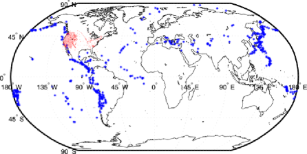
Figure 1: Distribution of the seismic wave sources (large earthquakes, blue) and receivers (seismic broadband stations, red) that generated our data. This is a regional tomography study that includes only data recorded in North America. In the mantle under this region, down to a few hundreds of kilometers depth, paths of incoming waves cross densely and from many directions, yielding good resolution for a three-dimensional imaging study.

everywhere inside the earth and at its surface. Figure 1 illustrates the spatial distribution of sources (large earthquakes, blue) and receivers (seismic broadband stations, red) that generated our data. Each datum $y_{i}$ measures the difference between an observed arrival time $y_{i}^{\mathrm{obs}}$ of a seismic wave $i$ and its predicted arrival time $y_{i}^{\mathrm{pred}}$:

$$y_{i}=y_{i}^{\mathrm{obs}}-y_{i}^{\mathrm{pred}}.$$

$y_{i}^{\mathrm{pred}}$ is evaluated using the spherically symmetric reference model IASP91 by Kennett and Engdahl (1991). For the teleseismic P waves used in our application, this difference $y_{i}$ would typically be on the order of one second, whereas $y_{i}^{\mathrm{obs}}$ and $y_{i}^{\mathrm{pred}}$ are on the order 600–1000 seconds. $y_{i}$ can be explained by slightly decreasing the modeled velocity in certain sub-volumes of the mantle.

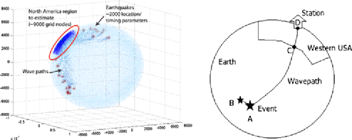
Figure 2: Physical setup and forward modeling of the seismic tomography problem. Left: parametrization of the spherical earth. Grid nodes are shown as blue dots. The goal is to estimate seismic velocity deviations $\bolds{\beta}$ at $\sim$9000 grid nodes under North America, inside the subvolume marked by the red ellipse. Red stars mark a few of the earthquake sources shown in Figure 1. The densified point clouds, between the sources and a few stations in North America, map out the sensitivity kernels of the selected wave paths. Each sensitivity kernel fills one row of matrix $X$. Left: schematic illustration of the components of an individual wave path.

We adopt the parametrization and a subset of the data measured by Sigloch, McQuarrie and Nolet (2008). The earth is meshed as a sphere of irregular tetrahedra with 92,175 mesh nodes. At each mesh mode, the parameters of interest are the relative velocity variation of the mantle with respect to the reference velocity of spherically-symmetric model IASP91 [Kennett and Engdahl (1991)]. The parameter vector is denoted as $\bolds{\beta}:=(\beta(\mathbf{r}),\mathbf{r}\in M_{\mathrm{Earth}})\in\mathbb{R}^{92{,}175}$, where the set of mesh node $M_{\mathrm{Earth}}$ fills the entire interior of the earth. Since both travel time deviations $y_{i}$ and the $\beta(\mathbf{r})$ are small, the wave equation may be linearized around the layered reference model:

$$y_{i}=\int\!\!\int\!\!\int_{\mathrm{Earth}}x_{i}(\mathbf{r})\beta(\mathbf{r})\,d^{3}\mathbf{r},$$ (1)

where $x_{i}(\mathbf{r})\in\mathbb{R}$ represents the Fréchet sensitivity kernel of the $i$th wavepath, that is, the partial derivatives of the chosen misfit measure or data $y_{i}$ with respect to the parameters $\beta(\mathbf{r})$. After numerical integration of kernel $x_{i}(\mathbf{r})$ onto the mesh, (1) takes the form

$$y_{i}=\sum_{\mathbf{r}\in M_{\mathrm{Earth}}}x_{i}(\mathbf{r})\beta(\mathbf{r})=\mathbf{x}_{i}^{\prime}\bolds{\beta}.$$ (2)

Geometrically speaking, row vector $\mathbf{x}_{i}^{\prime}$ maps out the mantle subvolume that would influence the travel time $y_{i}$ if some velocity anomaly $\beta(\mathbf{r})$ were located within it. This sensitivity region between an earthquake and a station essentially has ray-like character (Figure 2), though in physically more sophisticated approximations, the ray widens into a banana shape [Dahlen, Hung and Nolet (2000)]. Over the past decade, intense research effort has gone into the computability of sensitivity kernels under more and more realistic approximations [Dahlen, Hung and Nolet (2000), Tromp, Tape and Liu (2005), Tian et al. (2007), Nolet (2008)]. Since this issue is only tangential to our focus, we chose to keep the sensitivity calculations as simple as possible by modeling them as rays (the $\mathbf{x}_{i}^{\prime}$ are computed only once and stored). We note that the dependence of $x_{i}$ on $\bolds{\beta}$ can be neglected, as is common practice. This is justified by two facts: (i) velocity anomalies $\bolds{\beta}$ deviate from those of the (spherically symmetric) reference model by only a few percent, since the very mobile mantle does not support larger disequilibria, and (ii), even though the ray path in the true earth differs (slightly) from that in the reference model, this variation affects the travel time observable only to second order, according to Fermat’s principle [and analogous arguments for true finite-frequency sensitivities, Dahlen, Hung and Nolet (2000), Nolet (2008), Mercerat and Nolet (2013)]. Whatever the exact modeling is, it is very sparse, since every ray or banana visits only a small subvolume of the entire mantle—this sparsity is important for the computational efficiency of the MCMC sampling.

Gathering all $N$ observations, (2) can be rewritten as $\mathbf{y}=X\bolds{\beta}$, where sparse matrix $X\in\mathbb{R}^{N\times d}$ contains in its rows the $N$ sensitivity kernels. The left panel of Figure 2 illustrates the sensitivity kernels between one station and several earthquakes (i.e., several matrix rows). In practice, the problem never attains full rank, so that regularization must be added to remove the remaining nonuniqueness. The linear system $\mathbf{y}=X\bolds{\beta}$ is usually solved by some sparse matrix solver—a popular choice is the Sparse Equations and Least Squares (LSQR) algorithm by Paige and Saunders (1982), which minimizes $\|X\bolds{\beta}-\mathbf{y}\|^{2}+\lambda^{2}\|\bolds{\beta}\|^{2}$, where $\lambda$ is a regularization parameter that removes the underdeterminacy in $X$ [Montelli et al. (2004), Sigloch, McQuarrie and Nolet (2008), Tian, Sigloch and Nolet (2009), Dȩbski (2010)].

In summary, we have formulated the seismic tomography problem as it is overwhelmingly practiced by the geophysical community today. We use travel time differences $y_{i}$ as the misfit criterion, that is, as input data to the inverse problem, and seek to estimate the three-dimensional distribution of seismic velocity deviations $\bolds{\beta}$ that have caused these travel time anomalies. The sensitivity kernels $\mathbf{x}_{i}^{\prime}$ are modeled using ray theory, a high-frequency approximation to the full wave equation. In the conventional optimization approach, a regularization term is added, and the inverse problem is solved by minimizing the L2 norm misfit.

2.2 Setup of our example problem

Since all 92,175 velocity deviation parameters of the entire earth are currently not manageable for MCMC sampling, we regard as free parameters only 8977 of those parameters which are located beneath the western U.S., that is, between latitudes $20^{\circ}$N to $60^{\circ}$N, longitudes $90^{\circ}$W to $130^{\circ}$W, and 0–800 km depth. Tetrahedra nodes are spaced by 60–150 km. We denote this subset of velocity parameters as $\bolds{\beta}_{\mathrm{usa}}$.

Besides velocity parameters, we also consider the uncertainty in the location and the origin time of each earthquake source, which contribute to the travel time measurement. Government and research institutions routinely publish location estimates for every larger earthquake, but any event may easily be mistimed by a few seconds, and mislocated by ten or more kilometers (corresponding to a travel duration of 1 s or more). This is a problem, since the structural heterogeneities themselves only generate travel time delays on the order of a few seconds. Hence, the exact locations and timings of the earthquakes—or rather: their deviations from the published catalogue values—need to be treated as additional free parameters, to be estimated jointly with the structural parameters. These so-called “source corrections” are captured by three-dimensional shift corrections of the hypocenter ($\bolds{\beta}_{\mathrm{hyp}}$) and time corrections ($\bolds{\beta}_{\mathrm{time}}$) per earthquake.

Using the LSQR method, Sigloch, McQuarrie and Nolet (2008) jointly estimate all 92,175 parameters together with these “source corrections.” Using those LSQR solutions, we have two modeling alternatives for the earth structural inversion with $N$ travel delay time observations $\mathbf{y}\in\mathbb{R}^{N}$:

$$\mbox{{Model} 1:}\quad\mathbf{y}_{\mathrm{usa}}=X_{\mathrm{usa}}\bolds{\beta}_{\mathrm{usa}}+\bolds{\varepsilon},\qquad\bolds{\varepsilon}\sim\mathcal{N}_{N}\biggl{(}\mathbf{0},\frac{1}{\phi}I_{N}\biggr{)},$$ (3)

where $X_{\mathrm{usa}}\in\mathbb{R}^{N\times 8977}$ denotes the ensemble of sensitivity kernels of the western USA. $\mathcal{N}_{N}(\bolds{\mu},\Sigma)$ denotes the $N$-dimensional multivariate normal distribution with mean $\bolds{\mu}$ and covariance $\Sigma$, and the $N$-dimensional unity matrix is denoted by $I_{N}$. In model 1, we only estimate the velocity parameters $\bolds{\beta}_{\mathrm{usa}}$ and keep the part of the travel delay time for the corrections parameters (path AB in right panel of Figure 2) fixed at the LSQR solutions of $\bolds{\beta}_{\mathrm{hyp}}$ and $\bolds{\beta}_{\mathrm{time}}$ estimated by Sigloch, McQuarrie and Nolet (2008). The extended model with joint estimation of source corrections is given by

$$\mbox{{Model} 2:}\quad\mathbf{y}_{\mathrm{cr}} = X_{\mathrm{usa}}\bolds{\beta}_{\mathrm{usa}}+X_{\mathrm{hyp}}\bolds{\beta}_{\mathrm{hyp}}+X_{\mathrm{time}}\bolds{\beta}_{\mathrm{time}}+\bolds{\varepsilon},$$

$$\bolds{\varepsilon} \sim \mathcal{N}_{N}\biggl{(}\mathbf{0},\frac{1}{\phi}I_{N}\biggr{)}.$$

Here we apply the travel delay time $\mathbf{y}_{\mathrm{cr}}$ assuming that the part of the travel time running through path AC is given. This given part of the travel times is again based on the LSQR solution estimated by Sigloch, McQuarrie and Nolet (2008).

The number of travel time data from source-receiver pairs is $N=53\mbox{,}270$, collected from 760 stations and 529 events. The number of hypocenter correction parameters is 1587 (529 earthquakes${}\times{}$3) and there are 529 time correction parameters. Sigloch (2008) found that in the uppermost mantle, between 0 km to 100 km depth, the velocity can deviate by more than $\pm 5\%$ from the spherically symmetric reference model. As depth increases, the mantle becomes more homogeneous and the velocity deviates less from the reference model.

3 Estimation method

3.1 Modeling the spatial structure of the velocity parameters

In both models (3) and (2.2) we have the spatial parameter $\bolds{\beta}_{\mathrm{usa}}$, which we denote generically as $\bolds{\beta}$ in this section. In the Bayesian approach we need a proper prior distribution for this high-dimensional parameter vector $\bolds{\beta}$. To account for their spatially correlated structure, we apply the conditional autoregressive model (CAR) and assume a Markov random field structure for $\bolds{\beta}$. This assumption says that the conditional distribution of the local characteristics $\beta_{i}$, given all other parameters $\beta_{j}$, $j\neq i$, only depends on the neighbors, that is, $P(\beta_{i}\mid\bolds{\beta}_{-i})=P(\beta_{i}\mid\beta_{j},j\sim i)$, where $\bolds{\beta}_{-i}:=(\beta_{1},\ldots,\beta_{i-1},\beta_{i+1},\ldots,\beta_{d})^{\prime}$ and “$\sim$$i$” denotes the set of neighbors of site $i$. The CAR model and its application have been investigated in many studies, such as Pettitt, Weir and Hart (2002) or Rue and Held (2005). Since the earth is heterogeneous and layered, lateral correlation length scales are larger than over depths, and so we propose an ellipsoidal neighborhood structure for the velocity parameters. Let $(x_{j},y_{j},z_{j})^{\prime}\in\mathbb{R}^{3}$ be the positions of the $i$th and the $j$th nodes in Cartesian coordinates. The $j$th node is a neighbor of node $i$ if the ellipsoid equation is satisfied, that is, $(\frac{x_{i}-x_{j}}{D_{x}})^{2}+(\frac{y_{i}-y_{j}}{D_{y}})^{2}+(\frac{z_{i}-z_{j}}{D_{z}})^{2}\leq 1$. To add a rotation of the ellipsoid to an arbitrary direction in the space, we could simply modify the vector $(x_{i}-x_{j},y_{i}-y_{j},z_{i}-z_{j})^{\prime}$ to $R(x_{i}-x_{j},y_{i}-y_{j},z_{i}-z_{j})^{\prime}$ with a rotation matrix $R=R_{x}R_{y}R_{z}$ for given rotation matrices in the $x$, $y$ and $z$ directions, respectively. The spherical neighborhood structure is a special case of the ellipsoidal structure with $D_{x}=D_{y}=D_{z}$. Let $D$ be the maximum distance of $D_{x}$, $D_{y}$ and $D_{z}$. For weighting the neighbors we adopt either the exponential $w_{e}(\cdot)$ or reciprocal weight functions $w_{r}(\cdot)$, that is,

$$w_{e}(d_{ij}):=\exp\biggl{\{}-\frac{3d_{ij}^{2}}{D^{2}}\biggr{\}}\quad\mbox{and}\quad w_{r}(d_{ij}):=\frac{D}{d_{ij}}-1,$$ (5)

where $d_{ij}$ is the Euclidean distance between node $i$ and node $j$. The exponential weight function is bounded while the reciprocal weight function is unbounded. Those weighting functions have been studied by Pettitt, Weir and Hart (2002) or Congdon (2003). The left panel of Figure 3 illustrates the weight functions for $D=300$ km.

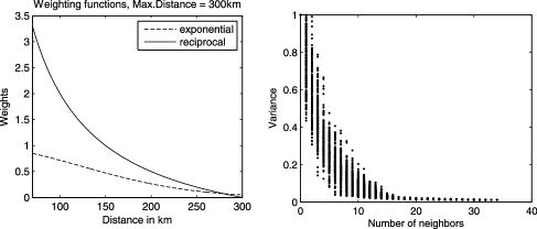
Figure 3: Left: exponential and reciprocal weight functions for the spatial prior, for $D=150$ km and $D=300$ km. Right: the trade-off relationship between numbers of neighbors and the prior variance $\operatorname{diag}(Q^{-1}(\psi)),\psi=10$, $D=150$ km, $w=\mbox{reciprocal}$ weights.

Let $\omega(d_{ij})$ be either $w_{e}(\cdot)$ or $w_{r}(\cdot)$ in (5). To model the spatial structure of $\bolds{\beta}_{\mathrm{usa}}$ in (3) and (2.2), a CAR model is used. Following Pettitt, Weir and Hart (2002), let $\bolds{\beta}_{\mathrm{usa}}\sim\mathcal{N}_{d_{\mathrm{usa}}}(\mathbf{0},\frac{1}{\eta_{\mathrm{usa}}}Q^{-1}(\psi))$ with precision matrix

$$Q_{ij}(\psi):=\cases{\displaystyle 1+|\psi|\sum_{i:j\sim i}\omega(d_{ij}),&\quad$i=j$,\vspace*{2pt}\cr\displaystyle-\psi\omega(d_{ij}),&\quad$i\neq j,i\sim j\mbox{ for }\psi\in\mathbb{R}$.}$$ (6)

They showed that $Q$ is symmetric and positive definite, and that conditional correlations can be explicitly determined. For $\psi\rightarrow 0$, the precision matrix $Q$ converges to the identity matrix, that is, $\psi=0$ corresponds to independent elements of $\bolds{\beta}$. The precision matrix in (6) for both elliptical and spherical cases indicates anisotropic covariance structure and depends on the distance between nodes, the number of neighbors of each node and the weighting functions. The elliptical precision matrix additionally depends on the orientation. The right panel of Figure 3 shows the trade-off between numbers of neighbors and prior variance, which indicates that the more neighbors the $i$th node has, the smaller is its prior variance $(Q^{-1}(\psi))_{ii}$. Posterior distribution of velocity parameters from regions with less neighborhood information can be rough, since they are not highly regularized due to the large prior covariances. This may produce sharp edges in the tomographic image. However, this is a more realistic modeling method since one is more sure about the optimization solution if a velocity parameter has more neighbors. Moreover, this prior specification is adapted to the construction of the tetrahedral mesh: regions with many nodes have better ray coverage than regions with less nodes. In summary, the prior incorporates diverse spatial knowledge about the velocity parameters. Since a precision matrix is defined, which is sparse and positive definite, it provides a computational advantage in sampling from a high-dimensional Gaussian distribution as required in our algorithm (shown in the following sections).

3.2 A Gibbs–Metropolis sampler for parameter estimation in high dimensions

To quantify uncertainty, we adopt a Bayesian approach. Posterior inference for the model parameters is facilitated by a Metropolis within Gibbs sampler [Brooks et al. (2011)]]. Recall the linear model in (2.2),

$$\mathbf{Y}=X\bolds{\beta}+\bolds{\varepsilon},\qquad\bolds{\varepsilon}\sim\mathcal{N}_{N}\biggl{(}\mathbf{0},\frac{1}{\phi}I_{N}\biggr{)},$$

where $\bolds{\beta}:=(\bolds{\beta}_{\mathrm{usa}},\bolds{\beta}_{\mathrm{hyp}},\bolds{\beta}_{\mathrm{time}})^{\prime}$ and $X:=(X_{\mathrm{usa}},X_{\mathrm{hyp}},X_{\mathrm{time}})$. We now specify the prior distribution of $\bolds{\beta}$ as

$$\bolds{\beta}\sim\mathcal{N}_{d}(\bolds{\beta}_{0},\Sigma_{\beta})\qquad\mbox{with }\bolds{\beta}_{0}:=(\bolds{\beta}_{0,\mathrm{usa}},\bolds{\beta}_{0,\mathrm{hyp}},\bolds{\beta}_{0,\mathrm{time}})^{\prime}.$$

The prior covariance matrix $\Sigma_{\beta}$ is chosen as

$$\Sigma_{\beta}:=\pmatrix{\displaystyle\frac{1}{\eta_{\mathrm{usa}}}Q^{-1}(\psi)&\mathbf{0}&\mathbf{0}\vspace*{2pt}\cr\mathbf{0}&\displaystyle\frac{1}{\eta_{\mathrm{hyp}}}I_{d_{\mathrm{hyp}}}&\mathbf{0}\vspace*{2pt}\cr\mathbf{0}&\mathbf{0}&\displaystyle\frac{1}{\eta_{\mathrm{time}}}I_{d_{\mathrm{time}}}}.$$ (7)

Since we are interested in modeling positive spatial dependence, we impose that the spatial dependence parameter $\psi$ is the truncated normal distribution a priori, that is, $\psi\sim\mathcal{N}(\mu_{\psi},\sigma^{2}_{\psi})\mathbh{1}(\psi>0)$. The priors for the precision scale parameters $\eta_{\mathrm{usa}}$, $\eta_{\mathrm{hyp}}$, $\eta_{\mathrm{time}}$ and $\phi$ are specified in terms of a Gamma distribution $\Gamma(a,b)$ with density $g(x;a,b)=\frac{b^{a}}{\Gamma(a)}x^{a-1}\exp\{-bx\}$, $x>0$. The corresponding first two moments are $\frac{a}{b}$ and $\frac{a}{b^{2}}$, respectively.

The MCMC procedure is derived as follows: the full conditionals of $\bolds{\beta}$ are

$$\bolds{\beta}\mid\mathbf{y},\psi,\bolds{\eta} \sim \mathcal{N}_{d}\bigl{(}\Omega_{\beta}^{-1}\bolds{\xi}_{\beta},\Omega_{\beta}^{-1}\bigr{)},$$ (9)

$$\eqntext{\mbox{with }\Omega_{\beta}:=\Sigma_{\beta}^{-1}+\phi X^{\prime}X,\bolds{\xi}_{\beta}:=\Sigma_{\beta}^{-1}\bolds{\beta}_{0}+\phi X^{\prime}\mathbf{y}}$$

and $\bolds{\eta}:=(\eta_{\mathrm{usa}},\eta_{\mathrm{hyp}},\eta_{\mathrm{time}})$. For $\eta_{\mathrm{usa}}$, $\eta_{\mathrm{hyp}}$, $\eta_{\mathrm{time}}$ and $\phi$, the full conditionals are again Gamma distributed. The estimation of $\psi$ requires a Metropolis–Hastings (MH) step. The logarithm of the full conditional of $\psi$ is proportional to

$$\log\pi(\psi\mid\mathbf{y},\bolds{\beta},\bolds{\eta}) \propto \frac{1}{2}\log\bigl{|}Q(\psi)\bigr{|}$$

$${}-\frac{\eta_{\mathrm{usa}}}{2}(\bolds{\beta}_{\mathrm{usa}}-\bolds{\beta}_{0,\mathrm{usa}})^{\prime}Q(\psi)(\bolds{\beta}_{\mathrm{usa}}-\bolds{\beta}_{0,\mathrm{usa}})$$

$${}-\frac{(\psi-\mu_{\psi})^{2}}{2\sigma_{\psi}^{2}}.$$

For the MH step, we choose a truncated normal random walk proposal for $\psi$ to obtain a new sample, that is, $\mathcal{N}(\psi^{\mathrm{old}},\bar{\sigma}_{\psi}^{2})\mathbh{1}(\psi>0)$. We use a Cholesky decomposition with permutation to obtain a sample of $\bolds{\beta}$ in (9) (Section 3.4). The method by Pettitt, Weir and Hart (2002), solving a sparse matrix equation, is not useful. Here, computing the determinant of the Cholesky factor of $Q(\psi)$ is much more efficient than calculating its eigenvalues, due to the size and sparseness of $Q(\psi)$.

3.3 Relationship to ridge regression

To show the relationship between our approach and ridge regression (also called Tikhonov regularization), we consider only model 1. For simplicity we neglect the notation “usa” in (3). The analysis is also applicable to model 2.

Let $\hat{\bolds{\beta}}{}^{\mathrm{ridge}}(\lambda):=(X^{\prime}X+\lambda I_{d})^{-1}X^{\prime}\mathbf{y}$ be the corresponding ordinary ridge regression (ORR) estimate with shrinkage parameter $\lambda$ [Hoerl and Kennard (1970), Swindel (1976), Dȩbski (2010)]. For given hyperparameters $\eta$, $\phi$ and $\psi$, the full conditional of $\bolds{\beta}$ is $\bolds{\beta}\mid\eta,\phi,\psi\sim\mathcal{N}_{d}(\Omega^{-1}_{\beta}\bolds{\xi}_{\beta},\Omega^{-1}_{\beta})$ with $\Omega_{\beta}:=\eta Q(\psi)+\phi X^{\prime}X$ and $\bolds{\xi}_{\beta}:=\eta Q(\psi)\bolds{\beta}_{0}+\phi X^{\prime}\mathbf{y}$. The corresponding full conditional mean can therefore be expressed as

$$E[\bolds{\beta}\mid\mathbf{y},\psi,\eta]=\biggl{(}X^{\prime}X+\frac{\eta}{\phi}Q(\psi)\biggr{)}^{-1}\biggl{(}X^{\prime}y+\frac{\eta}{\phi}Q(\psi)\bolds{\beta}_{0}\biggr{)}.$$

This is close to the modified ridge regression estimator $\hat{\bolds{\beta}}{}^{\mathrm{ridge}}(\lambda,\bolds{\beta}_{0}):=(X^{\prime}X+\lambda I_{d})^{-1}(X^{\prime}\mathbf{y}+\lambda\bolds{\beta}_{0})$ defined in Swindel (1976). We can see that if $\psi\rightarrow 0$, then $\frac{\eta}{\phi}Q(\psi)\rightarrow\frac{\eta}{\phi}$, which is the equivalent to $\lambda$ in the modified ridge regression. This shows that the prior precision matrix $\eta Q(\psi)$ is a regularization matrix with parameter $\psi$ controlling the prior covariance. As discussed in Section 3.1, the prior covariance $\frac{1}{\eta}Q^{-1}(\psi)$ also varies with the specified weights in (5) with maximum distance $D$ and with number of neighboring nodes. For large $\psi$ or large weights function values, as well as large number of neighbors, the prior variances are small, which well reflects the prior knowledge about the data coverage and parameter uncertainty. Thus, the full conditional mean is close to the prior mean in this case.

3.4 Computational issues

Since the size of the travel time data requires high-dimensional parameters to be estimated, the traditional method of sampling the parameter vector $\bolds{\beta}$ from $\mathcal{N}_{d}(\Omega_{\beta}^{-1}\bolds{\xi}_{\beta},\Omega_{\beta}^{-1})$ directly, as defined in (9), is not efficient with respect to computing time. We instead use a Cholesky decomposition of $\Omega_{\beta}$. Since the sensitivity kernel $X$ is sparse, and the prior covariance matrix is sparse and positive definite, the matrix $\Omega_{\beta}$ remains sparse and symmetric positive definite. Therefore, we can reduce the cost of the Cholesky decompositions. For this we apply an approximate minimum degree ordering algorithm (AMD algorithm) to find a permutation $P$ of $\Omega_{\beta}$ so that the number of nonzeros in its Cholesky factor is reduced [Amestoy, Davis and Duff (1996)]. In our case, the number of nonzeros of the full conditional precision matrix $\Omega_{\beta}$ in (9) is about $5\%$ of all elements. After this permutation the nonzeros of the Cholesky factor are reduced by $50\%$ compared to the original number of nonzeros.

To sample a multivariate normal distributed vector after permutation, we follow Rue and Held (2005). Given the permutation matrix $P$ of $\Omega_{\beta}$, we sample a vector $\mathbf{v}:=P\bolds{\beta}$, where $\mathbf{v}=(L_{p}^{\prime})^{-1}((L_{p}^{-1})P\bolds{\xi}_{\beta}+\mathbf{Z})$ with $L_{p}$ a lower triangular matrix resulting from the Cholesky decomposition of $P\Omega_{\beta,}$ and $\mathbf{Z}$ a standard normal distributed vector, that is, $\mathbf{Z}\sim\mathcal{N}_{d}(\mathbf{0},I_{d})$. The original parameter vector of interest $\bolds{\beta}$ can be obtained after permuting vector $\mathbf{v}$ again. Rue and Held (2005) suggested finding a permutation such that the matrix is banded. However, we found that in our case the AMD algorithm is more efficient with regard to computing time. Using MATLAB built-in functions, the Cholesky decomposition with an approximate minimum degree ordering takes 8 seconds on a Linux-Cluster 8-way Opteron with 32 cores, while the Cholesky decomposition based on a banded matrix takes 15 seconds. The traditional method without permutation requires 118.5 seconds.

4 Simulation study

4.1 Simulation setups

In this section we examine the performance of our approach for model 1. We want to investigate whether the method works correctly under the correct model assumptions and how much influence the prior has on the posterior estimation. We consider five different prior neighborhood structures of $\bolds{\beta}_{\mathrm{usa}}$:

(0) Independent model of $\bolds{\beta}_{\mathrm{usa}}$, $\psi=0$ fixed, that is, $\bolds{\beta}_{\mathrm{usa}}\sim\mathcal{N}_{d_{\mathrm{usa}}}(\bolds{\beta}_{0},\break\frac{1}{\eta_{\mathrm{usa}}}I_{d_{\mathrm{usa}}})$,

(1) Spherical neighborhood structure with reciprocal weight function,

(2) Ellipsoidal neighborhood structure with reciprocal weight function,

(3) Spherical neighborhood structure with exponential weight function,

(4) Ellipsoidal neighborhood structure with exponential weight function.

Note that the independent model of $\bolds{\beta}_{\mathrm{usa}}$ corresponds to the Bayesian ridge estimator as described in Section 3.3. For the weight functions in (5), we set $D_{x}=D_{y}=300$ km and $D_{z}=150$ km for modeling ellipsoidal neighborhood structures, and $D=150$ km for the spherical neighborhood distance.

Setup I: Assume the solution by Sigloch, McQuarrie and Nolet (2008), denoted as $\hat{\bolds{\beta}}{}^{\mathrm{LSQR}}_{\mathrm{usa}}$, represents true mantle structure beneath North America. We use the forward model $X\hat{\bolds{\beta}}{}^{\mathrm{LSQR}}_{\mathrm{usa}}$ to compute noise-free, synthetic data. Then, we generate two types of noisy data, that is, $\mathbf{Y}=\mathbf{X}\hat{\bolds{\beta}}{}^{\mathrm{LSQR}}_{\mathrm{usa}}+\bolds{\varepsilon}$ with:

(A) Gaussian noise ($\bolds{\varepsilon}\sim\mathcal{N}_{N}(\mathbf{0},\frac{1}{\phi_{\mathrm{tr}}}I_{N})$, $\phi_{\mathrm{tr}}=0.4$),

(B) $t$-noise ($\bolds{\varepsilon}\sim t_{N}(\mathbf{0},I_{N},\nu_{\mathrm{tr}})$, $\nu_{\mathrm{tr}}=3$, corresponds to $\phi_{\mathrm{tr}}=0.333$).

Although we add $t$-noise to our synthetic earth model $\hat{\bolds{\beta}}{}^{\mathrm{LSQR}}_{\mathrm{usa}}$, our posterior calculation is based on Gaussian errors. Additionally, we compare two priors for $\bolds{\beta}_{\mathrm{usa}}\sim\mathcal{N}_{d_{\mathrm{usa}}}(\bolds{\beta}_{0},\frac{1}{\eta_{\mathrm{usa}}}Q^{-1}(\psi))$ to examine the sensitivity of the posterior estimates to the prior choices:

(a) $\bolds{\beta}_{0}\sim\mathcal{N}_{d_{\mathrm{usa}}}(\hat{\bolds{\beta}}{}^{\mathrm{LSQR}}_{\mathrm{usa}},0.32^{2}I_{d})$,

(b) $\bolds{\beta}_{0}=\mathbf{0}$ (spherically symmetric reference model).

The priors for the hyperparameters are set as follows: $\psi\sim\mathcal{N}(10,0.2^{2})$, $\phi\sim{\Gamma}(1,0.1)$ resulting in expectation and standard deviation of 10, $\eta_{\mathrm{usa}}\sim{\Gamma}(10,2)$ resulting in expectation of 5 and standard deviation of 1.6.

Setup II: In this case we examine the performance under known prior neighborhood structures. We construct a synthetic true mantle model with two types of known prior neighborhood structures: $\bolds{\beta}_{\mathrm{usa},\mathrm{tr}}\sim\mathcal{N}_{d_{\mathrm{usa}}}(\hat{\bolds{\beta}}{}^{\mathrm{LSQR}}_{\mathrm{usa}},\break\frac{1}{\eta_{\mathrm{usa},\mathrm{tr}}}Q^{-1}(\psi_{\mathrm{tr}}))$ with $\eta_{\mathrm{usa},\mathrm{tr}}=0.18$ and $\psi_{\mathrm{tr}}=10$ using:

(a) a spherical neighborhood structure for $\bolds{\beta}_{\mathrm{usa},\mathrm{tr}}$ with reciprocal weights,

(b) an ellipsoidal neighborhood structure for $\bolds{\beta}_{\mathrm{usa},\mathrm{tr}}$ with reciprocal weights.

Again, Gaussian noise is added to the forward model, that is, $\mathbf{Y}=\break X\hat{\bolds{\beta}}{}^{\mathrm{LSQR}}_{\mathrm{usa}}+\bolds{\varepsilon}$, $\bolds{\varepsilon}\sim\mathcal{N}_{N}(0,\frac{1}{\phi_{\mathrm{tr}}}I_{N})$, $\phi_{\mathrm{tr}}=0.4$. Posterior estimation is carried out assuming the five different prior structures.

The number of MCMC iterations for scenarios in setups I and II is 3000, thinning is 15, and burn-in after thinning is 100. For convergence diagnostics we compute the trace, autocorrelation and estimated density plots as well as the effective sample size (ESS) using coda package in R for those samples. According to Brooks et al. (2011), the ESS is defined by $\mathrm{ESS}:=\frac{n}{1+2\sum_{k=1}^{\infty}\rho_{k}}$, with the original sample size $n$ and autocorrelation $\rho_{k}<0.05$ at lag $k$. The infinite sum can be truncated at lag $k$ when $\rho_{k}$ becomes smaller than 0.05 [Kass et al. (1998), Liu (2008)].

4.2 Performance evaluation measures

To evaluate the results, we use the standardized Euclidean norm for both data and model misfits, $\|\cdot\|_{\Sigma_{y}}$ and $\|\cdot\|_{\Sigma_{\beta}}$, respectively. The function $\|\mathbf{x}\|_{\Sigma}$ of a vector $\mathbf{x}$ of mean $\bolds{\mu}$ and covariance $\Sigma$ is called the Mahalanobis distance, defined by $\|\mathbf{x}\|_{\Sigma}:=\break\sqrt{(\mathbf{x}-\bolds{\mu})^{\prime}\Sigma^{-1}(\mathbf{x}-\bolds{\mu})}$. To include model complexity, we calculate the deviance information criterion (DIC) [Spiegelhalter et al. (2002)]. Let $\bolds{\theta}$ denote the parameter vector to be estimated. Furthermore, the likelihood of the model is denoted by $\ell(\mathbf{y}\mid\bar{\bolds{\theta}})$, where $\bar{\bolds{\theta}}$ is the estimated posterior mean of $\bolds{\theta}$, estimated by $\frac{1}{R}\sum_{r=1}^{R}\bolds{\theta}^{r}$ with $R$ number of independent MCMC samples. According to Spiegelhalter et al. (2002) and Celeux et al. (2006), the deviance is defined as $D(\bolds{\theta})=-2\log(\ell(\mathbf{y}\mid\bar{\bolds{\theta}}))+2\log h(\mathbf{y})$. The term $h(\mathbf{y})$ is a standardizing term which is a function of the data alone and does not need to be known. Thus, for model comparison we take $D(\bolds{\theta})=-2\log(\ell(\mathbf{y}\mid\bar{\bolds{\theta}}))$. The effective number of parameters in the model, denoted by $p_{D}$, is defined by $p_{D}:=E_{\theta}[D(\bolds{\theta})]-D(\bar{\bolds{\theta}})$. The term $E_{\theta}[D(\bolds{\theta})]$ is the posterior mean deviance and is estimated by $\frac{1}{R}\sum_{r=1}^{R}D(\bolds{\theta}^{r})$. This term can be regarded as a Bayesian measure of fit. In summary, the DIC is defined as $\mathrm{DIC}=E_{\theta}[D(\bolds{\theta})]+p_{D}=D(\bar{\bolds{\theta}})+2p_{D}$. The model with the smallest DIC is the preferred model under the trade-off of model fit and model complexity.

= Setup I Prior Mode Noises struct $\bolds{\|\mathbf{y}-X\hat{\bolds{\beta}}\|_{\Sigma_{y}}}$ $\bolds{\|\mathbf{y}-X\hat{\bolds{\beta}}_{L}\|_{\Sigma_{y}}}$ $\bolds{\|\mathbf{y}-X\hat{\bolds{\beta}}_{U}\|_{\Sigma_{y}}}$ $\bolds{\|\hat{\bolds{\beta}}-\bolds{\beta}_{\mathrm{tr}}\|_{\Sigma_{\beta}}}$ DIC $\bolds{\hat{\eta}_{\mathrm{usa}}}$ (a) $\bolds{\beta}\sim\mathcal{N}_{d}(\bolds{\beta}_{0},\frac{1}{\eta_{\mathrm{usa}}}Q^{-1}(\psi))$, $\bolds{\beta}_{0}\sim\mathcal{N}_{d}(\hat{\bolds{\beta}}{}^{\mathrm{LSQR}}_{\mathrm{usa}},0.32^{2}I_{d})$ (A) Gaussian noise (0) 232.28 312.82 308.27 $91.30$ 103,748 9.28    $\varepsilon_{i}\sim N(0,1/\phi_{\mathrm{tr}})$ (1) 231.71 258.32 255.74 $349.70$ 103,467 2.89    $\phi_{\mathrm{tr}}=0.4$, $\eta_{\mathrm{usa}}$, (2) 231.67 264.81 261.59 $200.34$ 103,442 0.11    $\psi$ unknown (3) 231.77 263.89 260.96 $256.52$ 103,478 2.70 (4) 231.70 267.81 264.44 $185.04$ 103,456 0.20 (B) $t$-noises (0) 227.74 602.35 604.21 $46.83$ 112,436 0.57    $\varepsilon_{i}\sim t(0,1,\nu_{\mathrm{tr}})$ (1) 228.58 443.00 443.02 $69.50$ 112,226 0.09    $\phi_{\mathrm{tr}}=0.33$, (2) 228.57 437.58 437.80 $57.83$ 112,118 0.01    $\nu_{\mathrm{tr}}=3$, $\eta_{\mathrm{usa}}$, (3) 228.51 450.67 450.27 $62.03$ 112,175 0.11    $\psi$ unknown (4) 228.52 445.22 445.42 $55.87$ 112,126 0.01 (b) $\bolds{\beta}\sim\mathcal{N}_{d}(\mathbf{0},\frac{1}{\eta_{\mathrm{usa}}}Q^{-1}(\psi))$ (A) Gaussian noise (0) 234.33 635.99 632.19 $50.53$ 106,563 0.59    $\varepsilon_{i}\sim N(0,1/\phi_{\mathrm{tr}})$ (1) 233.46 458.55 454.42 $40.53$ 105,365 0.09    $\phi_{\mathrm{tr}}=0.4$, $\eta_{\mathrm{usa}}$, (2) 233.36 449.35 444.06 $42.45$ 105,200 0.01    $\psi$ unknown (3) 233.52 466.36 462.04 $38.55$ 105,357 0.12 (4) 233.40 458.05 452.60 $42.71$ 105,256 0.01 (B) $t$-noises (0) 226.53 831.85 832.84 $40.10$ 113,023 0.19    $\varepsilon_{i}\sim t(0,1/\phi_{\mathrm{tr}},\nu_{\mathrm{tr}})$ (1) 227.60 599.53 598.99 $33.50$ 112,575 0.03    $\phi_{\mathrm{tr}}=0.33$, (2) 227.56 596.04 595.78 $33.62$ 112,512 0.00    $\nu_{\mathrm{tr}}=3$, $\eta_{\mathrm{usa}}$, (3) 227.61 606.60 605.77 $33.48$ 112,541 0.03    $\psi$ unknown (4) 227.55 607.03 606.69 $34.03$ 112,536 0.00

Table 1: Posterior estimation results of the simulation study under setups I and II, using synthetic earth models. The posterior mode of the velocity parameters is denoted as $\hat{\bolds{\beta}}$. The quantities $\hat{\bolds{\beta}}_{L}$ and $\hat{\bolds{\beta}}_{U}$ are lower and upper quantiles of the $90\%$ credible interval of the MCMC estimates, respectively

= Setup II Prior Mode Noises struct $\bolds{\|\mathbf{y}-X\hat{\bolds{\beta}}\|_{\Sigma_{y}}}$ $\bolds{\|\mathbf{y}-X\hat{\bolds{\beta}}_{L}\|_{\Sigma_{y}}}$ $\bolds{\|\mathbf{y}-X\hat{\bolds{\beta}}_{U}\|_{\Sigma_{y}}}$ $\bolds{\|\hat{\bolds{\beta}}-\bolds{\beta}_{\mathrm{tr}}\|_{\Sigma_{\beta}}}$ DIC $\bolds{\hat{\eta}_{\mathrm{usa}}}$ (a) $\bolds{\beta}\sim\mathcal{N}_{d}(\bolds{\beta}_{0},\frac{1}{\eta_{\mathrm{usa}}}Q^{-1}(\psi))$ with a spherical neighborhood structure for $Q$ Gaussian noise (0) 279.38 575.55 520.63 40.06 129,433 $1.09$    $\varepsilon_{i}\sim N(0,1/\phi_{\mathrm{tr}})$ (1) 279.82 439.32 389.22 35.83 128,882 $0.20$    $\phi_{\mathrm{tr}}=0.4$, (2) 279.78 475.57 422.49 36.95 129,034 $0.01$    $\eta_{\mathrm{usa}}=0.18$, (3) 279.96 455.81 404.30 36.23 128,986 $0.22$    $\psi=10$ (4) 279.79 481.30 427.90 37.10 129,066 $0.02$ (b) $\bolds{\beta}\sim\mathcal{N}_{d}(\bolds{\beta}_{0},\frac{1}{\eta_{\mathrm{usa}}}Q^{-1}(\psi))$ with an ellipsoidal neighborhood structure for $Q$ Gaussian noise (0) 234.71 305.10 292.47 27.71 104,662 $11.84$    $\varepsilon_{i}\sim N(0,1/\phi_{\mathrm{tr}})$ (1) 234.37 257.34 249.46 26.10 104,262 $4.19$    $\phi_{\mathrm{tr}}=0.4$, (2) 234.27 251.55 244.20 24.59 104,152 $0.30$    $\eta_{\mathrm{usa}}=0.18$, (3) 234.41 260.03 251.59 25.72 104,284 $4.22$    $\psi=10$ (4) 234.30 253.50 245.76 24.50 104,173 $0.53$

Table 1: (Continued)

4.3 Results and interpretations

The first two blocks in Table 1 illustrate posterior estimation results for setup I. It shows that the estimation method with ellipsoidal prior structures (2) and (4) turn out to be the most adequate, according to the DIC criterion. The standardized data misfit criteria $\|\cdot\|_{\Sigma_{y}}$ given the estimated posterior mode $\hat{\bolds{\beta}}$ show similar results in all scenarios. However, this measure ignores the uncertainty of $\bolds{\beta}_{\mathrm{usa}}$. The criteria $\|\mathbf{y}-X\hat{\bolds{\beta}}_{L}\|_{\Sigma_{y}}$ and $\|\mathbf{y}-X\hat{\bolds{\beta}}_{U}\|_{\Sigma_{y}}$ show the data misfit given the $90\%$ credible interval with lower and upper quantile posterior estimates $\hat{\bolds{\beta}}_{L}$ and $\hat{\bolds{\beta}}_{U}$, respectively. These estimates give a range of the data misfit for all possible posterior solutions of $\bolds{\beta}_{\mathrm{usa}}$ and show that methods with independent prior generally yield larger ranges of misfit values than the ones with spatial structures. This indicates that the credible intervals of methods with spatial priors can fit the data better. Further, methods with spatial priors in setup I(b) show smaller model misfit under $\|\cdot\|_{\Sigma_{\beta}}$ than ones with independent prior, while in setup I(a) results with independent priors are better. Generally, estimated posterior modes of $\eta_{\mathrm{usa}}$ vary considerably due to the different prior assumptions. Models with ellipsoidal neighborhood structures have a stronger prior (in the sense of a smaller prior variance) than models with spherical neighborhood structure. Similarly, models with reciprocal weights have a stronger regularization toward the prior mean than models with exponential weights. This means that the posterior estimates of $\eta_{\mathrm{usa}}$ adapt to different prior settings. Moreover, we notice that the estimate of the spatial dependence parameter $\psi$ depends strongly on its prior, as the prior mean is close to the posterior estimates of $\psi$ in all scenarios. The last two blocks in Table 1 illustrate results from setup II assuming known spatial structure including hyperparameters. The DIC values indicate that our approach correctly detects the underlying prior structures [in (a) it is prior structure (1), in (b) it is prior structure (2)]. We can also observe that our approach estimates the hyperparameters correctly. Estimated posterior modes of the parameters from the identified model are close to their true values.

Generally, tomographic images illustrate velocity parameters as deviation of the solution from the spherically symmetric reference model (in %). Blue colors represent zones that have faster seismic velocities than the reference earth model, while red colors denote slower velocities. Physically, blue colors usually imply that those regions are colder than the default expectation for the corresponding mantle depth, while red regions are hotter than expected. In our simulation study, we assumed the true earth to be represented by the solution of Sigloch, McQuarrie and Nolet (2008), shown in the left column of Figure 4. The middle and right columns of Figure 4 illustrate the estimated posterior modes $\hat{\bolds{\beta}}_{\mathrm{usa}}$ from setup I with ellipsoidal neighborhood structure and reciprocal weight for both Gaussian and $t$-noises, respectively. They show that the parameter estimates from Gaussian noises are close to the true solution, while the solution from the $t$-noises tends to overestimate the parameters. The magnitude of mantle anomalies is overestimated but major structures are correctly recovered. The same effect can be seen in the last column of Figure 4 which displays the estimated posterior modes of the tomographic solutions in setup I(b). We have overestimation since the noise is not adequate to the Gaussian model assumption. Moreover, we also observe that tomographic solutions with the prior mean $\bolds{\beta}_{0}\neq\mathbf{0}$ are smoother than the ones with the prior mean $\bolds{\beta}_{0}=\mathbf{0}$.

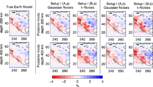
Figure 4: Mantle models resulting from the simulation study. Left column shows the “true” model, used to generate the synthetic data. The unit on the color bar is velocity deviation $\bolds{\beta}$ in % from the spherically symmetric reference model. All other columns show the posterior mode of velocity deviation $\bolds{\beta}$, estimated using ellipsoidal prior structure with reciprocal weights. Middle columns show results for setup I(a), which uses the prior mean $\bolds{\beta}\neq\mathbf{0}$. Right columns show results for setup I(b) assuming prior mean $\bolds{\beta}_{0}=\mathbf{0}$.

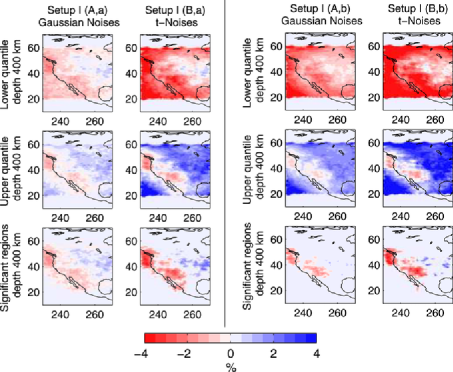
Figure 5: Continuation of Figure 4. The maps show velocity deviation in % from the reference Earth model. Left half shows the results under setup I(a), which uses the prior mean $\bolds{\beta}_{0}\neq\mathbf{0}$; right half describes setup I(b), which uses prior mean $\bolds{\beta}_{0}=\mathbf{0}$. First and second rows map out the lower and upper quantiles of the 90% confidence interval. Third row shows the posterior mode of velocity structure $\bolds{\beta}$, but rendered only in regions that differ significantly from the reference model, according to the 90% confidence interval.

Figure 5 shows estimated credible intervals for the solutions of Figure 4. Credible intervals for solutions with $t$-noises are larger than those for the Gaussian noises, as indicated by the darker shades of blue/red colors, which denote higher/lower quantile estimates. This implies that parameter uncertainty is greater if noise does not fit the model assumption. The same effect can be seen for results with the prior mean $\bolds{\beta}_{0}=\mathbf{0}$. The bottom row of Figure 5 maps out how the regions differ from the reference model with $90\%$ posterior probability. For model-conform Gaussian distributed noises and informative prior mean, more regions differ from the reference model with $90\%$ posterior probability than if we added $t$-noise or used the less informative prior. In the case of an informative prior and/or correctly modeled noise, we achieve more certainty about the velocity deviations from the reference earth model.

5 Application to real seismic travel time data

In this section we apply our MCMC approach to actually measured travel time data.

The measurements are a subset of those generated by Sigloch, McQuarrie and Nolet (2008). We use the same wave paths, but only measurements made on the broadband waveforms, whereas they further bandpassed the data for finite-frequency measurements and also included amplitude data [Sigloch and Nolet (2006)]. Most stations are located in the western U.S., as part of the largest-ever seismological experiment (USArray), which is still in the process of rolling across the continent from west to east. Numerous tomographic studies have incorporated USArray data—the ones most similar to ours are Burdick et al. (2008), Sigloch, McQuarrie and Nolet (2008), Tian, Sigloch and Nolet (2009), and Schmandt and Humphreys (2010). All prior studies obtained their solutions through least-squares minimization, which yields no uncertainty estimates. Here we use 53,270 broadband travel time observations to estimate velocity structure under western North America (over 11,000 parameters), plus source corrections for 529 events (2116 parameters). We conduct our Bayesian inversion following two different scenarios:

Model 1: We only invert for earth structural parameters. For the velocity parameters we assume $\bolds{\beta}\sim\mathcal{N}_{d_{\mathrm{usa}}}(\hat{\bolds{\beta}}{}^{\mathrm{LSQR}}_{\mathrm{usa}},\frac{1}{\eta_{\mathrm{usa}}}Q^{-1}(\psi))$ as in (3) with $\psi\sim\mathcal{N}(10,\allowbreak 0.5^{2})\mathbh{1}(\psi>0)$, $\phi\sim{\Gamma}(1,0.1)$ and $\eta_{\mathrm{usa}}\sim{\Gamma}(10,2)$.

Model 2: We invert for both earth structural parameters and the source corrections. The prior distributions are set to $\bolds{\beta}\sim\mathcal{N}_{d}(\hat{\bolds{\beta}}{}^{\mathrm{LSQR}},\Sigma_{\beta})$ as in (2.2) and $\Sigma_{\beta}$ as defined in (7). For $\psi$, $\phi$ and $\eta_{\mathrm{usa}}$, we adopt the same distribution as in model 1. For the parameters of the source corrections we adopt $\eta_{\mathrm{hyp}}\sim{\Gamma}(1,5)$ and $\eta_{\mathrm{time}}\sim{\Gamma}(10,2)$.

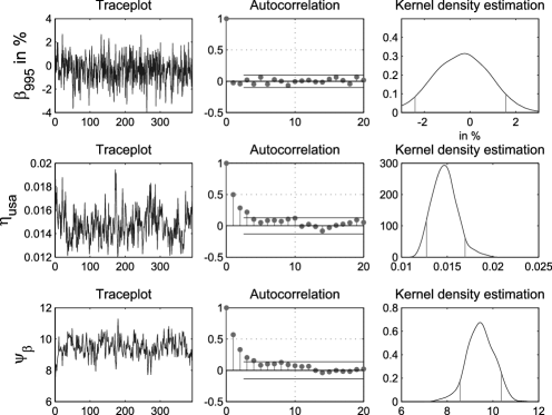
Figure 6: Convergence diagnostics: trace plot, autocorrelation and kernel density estimation of the parameters $\bolds{\beta}_{\mathrm{usa}}$ at node $955$, $\eta_{\mathrm{usa}}$ and $\psi_{\beta}$. For 10,000 MCMC iterations the samples shown in plots are based on a burn-in of 200 and a thinning rate of 25.

We use the same five prior structures (0)–(4) as in the simulation study and run the MCMC algorithm for 10,000 iterations. The high-dimensional $\bolds{\beta}$ vector can be sampled efficiently in terms of ESS with low burn-in and thinning rates thanks to the efficient Gibbs sampling scheme in (9). However, the hyperparameters, for example, $\psi_{\beta}$, are more difficult to sample. To achieve a good mixing, we applied a burn-in of 200 and a thinning rate of 25 (393 samples for each parameter) in our analysis. On average, the effective sample size ESS values for $\bolds{\beta}_{\mathrm{usa}}$, $\bolds{\beta}_{\mathrm{hyp}}$ and $\bolds{\beta}_{\mathrm{time}}$ are about $393$, $393$ and $327$, respectively, which indicate very low autocorrelations for most of the parameters. The ESS of both $\eta_{\mathrm{usa}}$ and $\psi_{\beta}$ is about 103, while both $\eta_{\mathrm{hyp}}$ and $\phi$ have good mixing characteristics with ESS values equal to the sample size, and $\eta_{\mathrm{time}}$ has ESS value equal to 165. Figure 6 shows as examples the parameters $\beta_{\mathrm{usa},955}$ at node $955$, $\eta_{\mathrm{usa}}$ and $\psi_{\beta}$. The computing cost of our algorithm is about $O(n^{4})$. Sampling model 1 with about 9000 parameters, our algorithm needs 12 hours in 10,000 runs on a 32-core cluster, while under the same condition it needs 38 hours for model 2.

Table 2: Posterior estimation results for the inversion using real data, under models 1 and 2 specifications

Model 1
Prior					Mode	Mode	Mode
struct	$\bolds{\|\mathbf{y}-X\hat{\bolds{\beta}}\|_{\Sigma_{y}}}$	$\bolds{\|\mathbf{y}-X\hat{\bolds{\beta}}_{L}\|_{\Sigma_{y}}}$	$\bolds{\|\mathbf{y}-X\hat{\bolds{\beta}}_{U}\|_{\Sigma_{y}}}$	DIC	$\bolds{\hat{\phi}}$	$\bolds{\hat{\eta}_{\mathrm{usa}}}$	$\bolds{\hat{\psi}}$
(0)	228.46	490.92	490.46	102,928	0.40	1.40	$-$
(1)	229.14	389.73	390.21	104,096	0.39	0.20	9.63
(2)	228.72	464.73	465.67	103,466	0.40	0.01	9.98
(3)	228.90	430.78	431.34	103,749	0.39	0.17	9.63
(4)	228.74	471.50	472.37	103,408	0.40	0.01	9.98

Model 2
Prior					Mode	Mode	Mode	Mode	Mode
struct	$\bolds{\|\mathbf{y}-X\hat{\bolds{\beta}}\|_{\Sigma_{y}}}$	$\bolds{\|\mathbf{y}-X\hat{\bolds{\beta}}_{L}\|_{\Sigma_{y}}}$	$\bolds{\|\mathbf{y}-X\hat{\bolds{\beta}}_{U}\|_{\Sigma_{y}}}$	DIC	$\bolds{\hat{\phi}}$	$\bolds{\hat{\eta}_{\mathrm{usa}}}$	$\bolds{\hat{\psi}}$	$\bolds{\hat{\eta}_{\mathrm{hyp}}}$	$\bolds{\hat{\eta}_{\mathrm{time}}}$
(0)	225.40	483.96	488.35	93,788	0.49	1.15	$-$	0.01	5.01
(1)	225.76	515.29	524.61	94,993	0.48	0.10	$9.63$	0.01	4.53
(2)	225.48	498.96	501.45	94,374	0.48	0.00	$9.55$	0.01	4.70
(3)	225.61	503.20	512.01	94,669	0.48	0.11	$9.63$	0.01	4.53
(4)	225.44	496.69	498.97	94,312	0.49	0.01	$10.00$	0.01	4.70

Table 2 shows the results from model 1 (estimation of earth structure) and model 2 (earth structure plus source corrections). For both models, results from the independent prior structures, corresponding to the Bayesian ridge estimator, provide the best fit according to the DIC criterion. We also run the model 1 with prior mean $\bolds{\beta}_{0}=\mathbf{0}$ (the spherically symmetric reference model) and different covariance structures (0)–(2). The DIC results for priors (0), (1) and (2) are 103,100, 103,700 and 103,370, respectively. Two reasons may explain the selection of prior (0): (1) the data has generally more correlation structure than the i.i.d. Gaussian assumption, which can not be solely explained by the spatial prior structure of the $\bolds{\beta}$-fields. However, in our simulation study where different prior structures and the corrected data error are applied (Table 1), the DIC was able to identify the correct models; (2) Since the data are noisy, fitting could be difficult without a shrinkage prior. The prior in (0) can be compared to shrinkage in the ridge regression, which is the limiting case of priors in (1) to (4). Priors in (1) to (4) do not shrink the solutions of $\bolds{\beta}$-fields as much as prior (0). They better reflect the uncertainty since the prior covariances in (1)–(4) are larger than variances in prior (0) in regions that have no data (no neighboring nodes), and smaller in regions with lots of data (lots of neighboring nodes).

Furthermore, the standardized data misfit criteria $\|\cdot\|_{\Sigma_{y}}$ do not show much difference between models with different prior specifications. According to the estimated $90\%$ credible interval, estimates using spherical prior structure show a smaller range of data misfit in model 1, whereas in model 2, the independence prior shows a better result. Since our method assumes i.i.d. Gaussian errors, the resulting residuals might not be optimally fitted as expected. With regard to computational time, the independent prior model has a definite advantage over other priors in both models 1 and 2. The general advantage of our Bayesian method is that the independent model yields an estimate given as the ratio between the variance of the data and the variance of the priors corresponding to ridge estimates with automatically chosen shrinkage described in Section 3.3, whereas in Aster, Borchers and Thurber (2005), Sigloch, McQuarrie and Nolet (2008), Bodin et al. (2012a) and all other prior work, the shrinkage parameter (strength of regularization) had to be chosen by the user a priori.

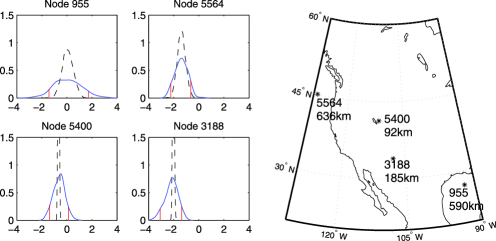
Figure 7: Results of the Bayesian tomography using real travel time observations. Left: estimated posterior density of $\bolds{\beta}_{\mathrm{usa}}$ at a few selected model nodes, whose locations and depths are indicated on the map. Unit on the x-axes is velocity deviation in %. Dashed lines: prior density, the prior variance can be very small if number of neighbors is large. Solid lines: posterior density with $90\%$ credible intervals.

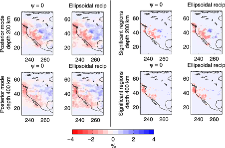
Figure 8: Results of the Bayesian tomography using real travel time data. All maps show estimated velocity deviation from the reference earth model IASP91 (in $\%$). Left columns: estimated posterior mode of velocity deviation, for the scenario of model 2. Right columns: same posterior mode, but rendered are only regions that differ from the reference model with $90\%$ posterior probability.

Figure 7 shows the estimated posterior and prior densities of parameters in model 2, at four different locations of varying depth. We see that parameters at locations with good ray coverage, for example, node 5400 and node 3188, have smaller credible intervals than parameters at locations with no ray coverage, for example, node 5564 and node 995 beneath the uninstrumented oceans. Geologically, the regions between node 5400 and node 3188 are well known to represent the hot upper mantle, where seismic waves travel slower than the reference velocity. This is consistent with our results in Figure 7: the fact that $\bolds{\beta}=\mathbf{0}$ does not fall inside the $90\%$ credible intervals indicates a velocity deviation from the spherically symmetric reference model with high posterior probability. Figure 7 shows that the posterior is more diffuse than the prior. As mentioned in Section 3.1, the spatial prior for $\bolds{\beta}$ depends on distance of neighboring nodes, number of neighbors and orientation. The variance can be very small if the number of neighbors is very large, as shown in Figure 3. Incorporating data, the information about $\bolds{\beta}$ is updated and thus may yield more diffuse posteriors than the priors, as we see here. The left half of Figure 8 shows the estimated posterior modes of mantle structure obtained by model 2, for independent and for ellipsoidal priors with reciprocal weights. The right half of Figure 8 extracts only those regions that differ from the reference model according to the $90\%$ credible interval. The ellipsoidal prior results in higher certainty of velocity deviations at a depth of 200 km compared to the independence prior. At a depth of 400 km, the credible regions resemble each other more strongly. This confirms geological arguments that deeper regions of the mantle are more homogeneous and do not differ as much from the spherically symmetric reference model as shallower regions.

Many lines of geoscientific investigations provide independent confirmation of the significantly anomalous regions of Figure 8. The red areas map out the hot upper mantle under the volcanic, extensional Basin and Range province and Yellowstone; the blue anomalies map out the western edge of the old and cool North American craton.

The overall comparison of our solutions to earlier least-squares inversions, for example, the model by Sigloch (2008) shown in the left column of Figure 4, confirms that Bayesian inversion successfully retrieves the major features of mantle structure. The images are similar, but the major advantage and novelty of our approach is that it also quantifies uncertainties in the solution (which we have chosen to visualize as credible intervals here).

6 Discussion and outlook

Uncertainty quantification in underdetermined, large inverse problems is important, since a single solution is not sufficient for making conclusive judgements. Two central difficulties for MCMC methods have always been the dimensionality of the problem (number of parameters to sample) or the evaluation of the complex physical forward model (nonlinear problems) in each MCMC iteration [Tarantola (2004), Bui-Thanh, Ghattas and Higdon (2011), Martin et al. (2012)].

Consider the model $\mathbf{Y}=f(\bolds{\beta})+\bolds{\varepsilon}$ with the physical forward model $f(\cdot)$, high-dimensional parameter $\bolds{\beta}$ and error $\bolds{\varepsilon}$. In general, if the physical problem is linear $(f(\bolds{\beta})=X\bolds{\beta})$ and the full conditional of $\bolds{\beta}$ is Gaussian, efficient sampling from the high-dimensional Gaussian conditional distribution is essential for the exploration of model space. In this case the error $\bolds{\varepsilon}$ need not necessarily be Gaussian, but may be $t$ or skewed-$t$ distributed [Sahu, Dey and Branco (2003), Frühwirth-Schnatter and Pyne (2010)], or a Gaussian error with a spatial correlation such as considered in Banerjee, Gelfand and Carlin (2003). Given a sparse posterior precision matrix [e.g., (9)], efficient sampling from a multivariate normal can be carried out by Cholesky decomposition of a permuted precision matrix as discussed in Wilkinson and Yeung (2002) or Rue and Held (2005), by using an approximate minimum-degree ordering algorithm. A further improvement to the current sampling approach might be to apply the Krylov subspace method from Simpson, Turner and Pettitt (2008). This would require substantial implementation efforts and is the subject of further research. If the forward matrix or the prior precision matrix is not sparse, a dense posterior precision matrix for $\bolds{\beta}$ will result. In this case our sampling scheme is inefficient, but the model-space reduction method developed by Flath et al. (2011) might be used instead. They exploit the low-rank structure of the preconditioned Hessian matrix of the data misfit, involving eigenvalue calculations. However, this approximation quantifies uncertainty of large-scale linear inverse problems only for known hyperparameters, thus ignoring uncertainty in those parameters. Eigenvalue calculation in each MCMC step can be time consuming and prohibitive for hierarchical models with unknown hyperparameters when the posterior covariance matrix in every MCMC step changes. Here additional research is needed.

If the full conditionals cannot be written as Gaussian [this case includes the cases of a nonlinear $f(\cdot)$, a non-Gaussian prior of $\bolds{\beta}$ or non-Gaussian, nonelliptical distributed errors], using the standard MH algorithm to sample from the high-dimensional posterior distribution is often computationally infeasible. Constructing proposal density that provides a good approximation of the stationary distribution while keeping the high-dimensional forward model $f(\cdot)$ inexpensive to evaluate has been the focus of the research over the past years: Lieberman, Willcox and Ghattas (2010) have drawn samples from an approximate posterior density on a reduced parameter space using a projection-based reduced-order model. In the adaptive rejection sampling technique by Cui, Fox and O’Sullivan (2011), the exact posterior density is evaluated only if its approximation is accepted. The stochastic Newton approach proposed by Martin et al. (2012) approximates the posterior density by local Hessian information, thus resulting in an improvement of the Langevin MCMC by Stramer and Tweedie (1999). Other random-walk-free, optimization-based MCMC techniques for improving the proposal and reducing correlation between parameters have been developed, such as Hamiltonian Monte Carlo (HMC) [Neal (2010)], Adaptive Monte Carlo (AM) [Haario, Saksman and Tamminen (2001), Andrieu and Thoms (2008)] and several variations, for example, delay rejection AM (DRAM) [Haario et al. (2006)], differential evolution MC (DEMC) [Ter Braak (2006)] and differential evolution adaptive Metropolis (DREAM) [Vrugt et al. (2009)], just to mention a few. However, MCMC sampling of high-dimensional problems still requires a massive amount of computing time and resources. For example, the quasi three-dimensional nonlinear model of Herbei, McKeague and Speer (2008) contains about 9000 parameters on a $37\times 19$ grid. We expect a long computing time since they use standard MCMC sampling methods. The example by Cui, Fox and O’Sullivan (2011) shows that their algorithm achieves a significant improvement in both computing time and efficiency of parameter space sampling for a large nonlinear system of PDEs that includes about 10,000 parameters. However, their algorithm gives 11,200 iterations in about 40 days, while our problem requires only 38 hours (on a 32-core cluster) for the same number of iterations for about 11,000 parameters.

While the future may be in effective uncertainty quantification of nonlinear physical problems using model reduction and optimization techniques, the computing time and resources at the moment are too demanding to explore the large model space. This paper demonstrates effective Bayesian analysis tailored to a realistically large seismic tomographic problem, featuring over 11,000 structural and source parameters. We deliver a precise uncertainty quantification of tomographic models in terms of posterior distribution and credible intervals using the MCMC samples, which allows us to detect regions that differ from the reference earth model with high posterior probability. Our approach is the first to solve seismic tomographic problems in such high dimensions on a fine grid, and thus provides ground work in this important research area.

References

- Aki and Lee (1976) {barticle}[author] \bauthor\bsnmAki, \bfnmK.\binitsK. and \bauthor\bsnmLee, \bfnmW.\binitsW. (\byear1976). \btitleDetermination of three-dimensional velocity anomalies under a seismic array using first P arrival times from local earthquakes: 1. A homogeneous initial model. \bjournalJournal of Geophysical Research \bvolume81 \bpages4381–4399. \bptokimsref \endbibitem
- Amestoy, Davis and Duff (1996) {barticle}[mr] \bauthor\bsnmAmestoy, \bfnmPatrick R.\binitsP. R., \bauthor\bsnmDavis, \bfnmTimothy A.\binitsT. A. and \bauthor\bsnmDuff, \bfnmIain S.\binitsI. S. (\byear1996). \btitleAn approximate minimum degree ordering algorithm. \bjournalSIAM J. Matrix Anal. Appl. \bvolume17 \bpages886–905. \biddoi=10.1137/S0895479894278952, issn=0895-4798, mr=1410707 \bptokimsref \endbibitem
- Andrieu and Thoms (2008) {barticle}[mr] \bauthor\bsnmAndrieu, \bfnmChristophe\binitsC. and \bauthor\bsnmThoms, \bfnmJohannes\binitsJ. (\byear2008). \btitleA tutorial on adaptive MCMC. \bjournalStat. Comput. \bvolume18 \bpages343–373. \biddoi=10.1007/s11222-008-9110-y, issn=0960-3174, mr=2461882 \bptokimsref \endbibitem
- Aster, Borchers and Thurber (2005) {bbook}[author] \bauthor\bsnmAster, \bfnmRichard\binitsR., \bauthor\bsnmBorchers, \bfnmBrian\binitsB. and \bauthor\bsnmThurber, \bfnmClifford\binitsC. (\byear2005). \btitleParameter Estimation and Inverse Problems (International Geophysics), \beditionHar/cdr ed. \bpublisherAcademic Press, \blocationSan Diego. \bptokimsref \endbibitem
- Banerjee, Gelfand and Carlin (2003) {bbook}[author] \bauthor\bsnmBanerjee, \bfnmS.\binitsS., \bauthor\bsnmGelfand, \bfnmA. E.\binitsA. E. and \bauthor\bsnmCarlin, \bfnmB. P.\binitsB. P. (\byear2003). \btitleHierarchical Modeling and Analysis for Spatial Data. \bpublisherChapman & Hall/CRC, \blocationBoca Raton, FL. \bptokimsref \endbibitem
- Bardsley (2012) {barticle}[mr] \bauthor\bsnmBardsley, \bfnmJohnathan M.\binitsJ. M. (\byear2012). \btitleMCMC-based image reconstruction with uncertainty quantification. \bjournalSIAM J. Sci. Comput. \bvolume34 \bpagesA1316–A1332. \biddoi=10.1137/11085760X, issn=1064-8275, mr=2970254 \bptokimsref \endbibitem
- Bodin and Sambridge (2009) {barticle}[author] \bauthor\bsnmBodin, \bfnmT.\binitsT. and \bauthor\bsnmSambridge, \bfnmM.\binitsM. (\byear2009). \btitleSeismic tomography with the reversible jump algorithm. \bjournalGeophysical Journal International \bvolume178 \bpages1411–1436. \bptokimsref \endbibitem
- Bodin et al. (2012a) {barticle}[author] \bauthor\bsnmBodin, \bfnmT.\binitsT., \bauthor\bsnmSambridge, \bfnmM.\binitsM., \bauthor\bsnmTkalčić, \bfnmH.\binitsH., \bauthor\bsnmArroucau, \bfnmP.\binitsP., \bauthor\bsnmGallagher, \bfnmK.\binitsK. and \bauthor\bsnmRawlinson, \bfnmN.\binitsN. (\byear2012a). \btitleTransdimensional inversion of receiver functions and surface wave dispersion. \bjournalJournal of Geophysical Research \bvolume117 \bpagesB02301. \bptokimsref \endbibitem
- Bodin et al. (2012b) {barticle}[author] \bauthor\bsnmBodin, \bfnmThomas\binitsT., \bauthor\bsnmSambridge, \bfnmMalcolm\binitsM., \bauthor\bsnmRawlinson, \bfnmNick\binitsN. and \bauthor\bsnmArroucau, \bfnmPierre\binitsP. (\byear2012b). \btitleTransdimensional tomography with unknown data noise. \bjournalGeophysical Journal International \bvolume189 \bpages1536–1556. \bptokimsref \endbibitem
- Brooks et al. (2011) {bbook}[mr] \beditor\bsnmBrooks, \bfnmSteve\binitsS., \beditor\bsnmGelman, \bfnmAndrew\binitsA., \beditor\bsnmJones, \bfnmGalin L.\binitsG. L. and \beditor\bsnmMeng, \bfnmXiao-Li\binitsX.-L., eds. (\byear2011). \btitleHandbook of Markov Chain Monte Carlo. \bpublisherCRC Press, \blocationBoca Raton, FL. \biddoi=10.1201/b10905, mr=2742422 \bptokimsref \endbibitem
- Bui-Thanh, Ghattas and Higdon (2011) {bmisc}[author] \bauthor\bsnmBui-Thanh, \bfnmTan\binitsT., \bauthor\bsnmGhattas, \bfnmOmar\binitsO. and \bauthor\bsnmHigdon, \bfnmDavid\binitsD. (\byear2011). \bhowpublishedAdaptive Hessian-based non-stationary Gaussian process response surface method for probability density approximation with application to Bayesian solution of large-scale inverse problems. Technical report, Institut for computational engineering and sciences, Univ. Texas, Austin. \bptokimsref \endbibitem
- Burdick et al. (2008) {barticle}[author] \bauthor\bsnmBurdick, \bfnmScott\binitsS., \bauthor\bsnmLi, \bfnmChang\binitsC., \bauthor\bsnmMartynov, \bfnmVladik\binitsV., \bauthor\bsnmCox, \bfnmTrilby\binitsT., \bauthor\bsnmEakins, \bfnmJennifer\binitsJ., \bauthor\bsnmMulder, \bfnmTaimi\binitsT., \bauthor\bsnmAstiz, \bfnmLuciana\binitsL., \bauthor\bsnmVernon, \bfnmFrank L.\binitsF. L., \bauthor\bsnmPavlis, \bfnmGary L.\binitsG. L. and \bauthor\bparticlevan der \bsnmHilst, \bfnmRobert D.\binitsR. D. (\byear2008). \btitleUpper mantle heterogeneity beneath North America from travel time tomography with global and USArray transportable array data. \bjournalSeismological Research Letters \bvolume79 \bpages389–392. \bptokimsref \endbibitem
- Celeux et al. (2006) {barticle}[mr] \bauthor\bsnmCeleux, \bfnmG.\binitsG., \bauthor\bsnmForbes, \bfnmF.\binitsF., \bauthor\bsnmRobert, \bfnmC. P.\binitsC. P. and \bauthor\bsnmTitterington, \bfnmD. M.\binitsD. M. (\byear2006). \btitleDeviance information criteria for missing data models. \bjournalBayesian Anal. \bvolume1 \bpages651–673 (electronic). \biddoi=10.1214/06-BA122, issn=1931-6690, mr=2282197 \bptokimsref \endbibitem
- Congdon (2003) {bbook}[mr] \bauthor\bsnmCongdon, \bfnmPeter\binitsP. (\byear2003). \btitleApplied Bayesian Modelling. \bpublisherWiley, \blocationChichester. \biddoi=10.1002/0470867159, mr=1990543 \bptokimsref \endbibitem
- Crosson (1976) {barticle}[author] \bauthor\bsnmCrosson, \bfnmRobert S.\binitsR. S. (\byear1976). \btitleCrustal structure modeling of earthquake data 1. Simultaneous least squares estimation of hypocenter and velocity parameters. \bjournalJournal of Geophysical Research \bvolume81 \bpages3036–3046. \bptokimsref \endbibitem
- Cui, Fox and O’Sullivan (2011) {barticle}[author] \bauthor\bsnmCui, \bfnmT.\binitsT., \bauthor\bsnmFox, \bfnmC.\binitsC. and \bauthor\bsnmO’Sullivan, \bfnmM. J.\binitsM. J. (\byear2011). \btitleBayesian calibration of a large-scale geothermal reservoir model by a new adaptive delayed acceptance Metropolis–Hastings algorithm. \bjournalWater Resources Research \bvolume47 \bpages26 pp. \bptokimsref \endbibitem
- Dahlen, Hung and Nolet (2000) {barticle}[author] \bauthor\bsnmDahlen, \bfnmF. A.\binitsF. A., \bauthor\bsnmHung, \bfnmS. H.\binitsS. H. and \bauthor\bsnmNolet, \bfnmGuust\binitsG. (\byear2000). \btitleFréhet kernels for finite-frequency traveltimes-I. Theory. \bjournalGeophysical Journal International \bvolume141 \bpages157–174. \bptokimsref \endbibitem
- Dȩbski (2010) {barticle}[author] \bauthor\bsnmDȩbski, \bfnmWojciech\binitsW. (\byear2010). \btitleSeismic tomography by Monte Carlo sampling. \bjournalPure and Applied Geophysics \bvolume167 \bpages131–152. \bptokimsref \endbibitem
- Dziewonski and Anderson (1981) {barticle}[author] \bauthor\bsnmDziewonski, \bfnmA. M.\binitsA. M. and \bauthor\bsnmAnderson, \bfnmD. L.\binitsD. L. (\byear1981). \btitlePreliminary reference Earth model. \bjournalPhysics of the Earth and Planetary Interiors \bvolume25 \bpages297–356. \bptokimsref \endbibitem
- Fichtner et al. (2009) {barticle}[author] \bauthor\bsnmFichtner, \bfnmA.\binitsA., \bauthor\bsnmKennett, \bfnmB. L. N.\binitsB. L. N., \bauthor\bsnmIgel, \bfnmH.\binitsH. and \bauthor\bsnmBunge, \bfnmH. P\binitsH. P. (\byear2009). \btitleFull waveform tomography for upper-mantle structure in the Australasian region using adjoint methods. \bjournalGeophysical Journal International \bvolume179 \bpages1703–1725. \bptokimsref \endbibitem
- Flath et al. (2011) {barticle}[mr] \bauthor\bsnmFlath, \bfnmH. P.\binitsH. P., \bauthor\bsnmWilcox, \bfnmL. C.\binitsL. C., \bauthor\bsnmAkçelik, \bfnmV.\binitsV., \bauthor\bsnmHill, \bfnmJ.\binitsJ., \bauthor\bparticlevan \bsnmBloemen Waanders, \bfnmB.\binitsB. and \bauthor\bsnmGhattas, \bfnmO.\binitsO. (\byear2011). \btitleFast algorithms for Bayesian uncertainty quantification in large-scale linear inverse problems based on low-rank partial Hessian approximations. \bjournalSIAM J. Sci. Comput. \bvolume33 \bpages407–432. \biddoi=10.1137/090780717, issn=1064-8275, mr=2783201 \bptokimsref \endbibitem
- Frühwirth-Schnatter and Pyne (2010) {barticle}[author] \bauthor\bsnmFrühwirth-Schnatter, \bfnmS.\binitsS. and \bauthor\bsnmPyne, \bfnmS.\binitsS. (\byear2010). \btitleBayesian inference for finite mixtures of univariate and multivariate skew-normal and skew- distributions. \bjournalBiostatistics \bvolume11 \bpages317–336. \bptokimsref \endbibitem
- Haario, Saksman and Tamminen (2001) {barticle}[mr] \bauthor\bsnmHaario, \bfnmHeikki\binitsH., \bauthor\bsnmSaksman, \bfnmEero\binitsE. and \bauthor\bsnmTamminen, \bfnmJohanna\binitsJ. (\byear2001). \btitleAn adaptive metropolis algorithm. \bjournalBernoulli \bvolume7 \bpages223–242. \biddoi=10.2307/3318737, issn=1350-7265, mr=1828504 \bptokimsref \endbibitem
- Haario et al. (2006) {barticle}[mr] \bauthor\bsnmHaario, \bfnmHeikki\binitsH., \bauthor\bsnmLaine, \bfnmMarko\binitsM., \bauthor\bsnmMira, \bfnmAntonietta\binitsA. and \bauthor\bsnmSaksman, \bfnmEero\binitsE. (\byear2006). \btitleDRAM: Efficient adaptive MCMC. \bjournalStat. Comput. \bvolume16 \bpages339–354. \biddoi=10.1007/s11222-006-9438-0, issn=0960-3174, mr=2297535 \bptokimsref \endbibitem
- Hämäläinen and Ilmoniemi (1994) {barticle}[author] \bauthor\bsnmHämäläinen, \bfnmM. S.\binitsM. S. and \bauthor\bsnmIlmoniemi, \bfnmR. J.\binitsR. J. (\byear1994). \btitleInterpreting magnetic fields of the brain: Minimum norm estimates. \bjournalMedical and Biolgical Engineering and Computing \bvolume32 \bpages35–42. \bptokimsref \endbibitem
- Herbei, McKeague and Speer (2008) {barticle}[author] \bauthor\bsnmHerbei, \bfnmRadu\binitsR., \bauthor\bsnmMcKeague, \bfnmIan W.\binitsI. W. and \bauthor\bsnmSpeer, \bfnmKevin G.\binitsK. G. (\byear2008). \btitleGyres and jets: Inversion of tracer data for ocean circulation structure. \bjournalJournal of Physical Oceanography \bvolume38 \bpages1180–1202. \bptokimsref \endbibitem
- Hoerl and Kennard (1970) {barticle}[author] \bauthor\bsnmHoerl, \bfnmE.\binitsE. and \bauthor\bsnmKennard, \bfnmRobert W.\binitsR. W. (\byear1970). \btitleRidge regression: Biased estimation for nonorthogonal problems. \bjournalTechnometrics \bvolume12 \bpages55–67. \bptokimsref \endbibitem
- Kaipio and Somersalo (2007) {barticle}[mr] \bauthor\bsnmKaipio, \bfnmJari\binitsJ. and \bauthor\bsnmSomersalo, \bfnmErkki\binitsE. (\byear2007). \btitleStatistical inverse problems: Discretization, model reduction and inverse crimes. \bjournalJ. Comput. Appl. Math. \bvolume198 \bpages493–504. \biddoi=10.1016/j.cam.2005.09.027, issn=0377-0427, mr=2260683 \bptokimsref \endbibitem
- Kass et al. (1998) {barticle}[mr] \bauthor\bsnmKass, \bfnmRobert E.\binitsR. E., \bauthor\bsnmCarlin, \bfnmBradley P.\binitsB. P., \bauthor\bsnmGelman, \bfnmAndrew\binitsA. and \bauthor\bsnmNeal, \bfnmRadford M.\binitsR. M. (\byear1998). \btitleMarkov chain Monte Carlo in practice: A roundtable discussion. \bjournalAmer. Statist. \bvolume52 \bpages93–100. \biddoi=10.2307/2685466, issn=0003-1305, mr=1628427 \bptokimsref \endbibitem
- Kennett and Engdahl (1991) {barticle}[author] \bauthor\bsnmKennett, \bfnmB. L. N.\binitsB. L. N. and \bauthor\bsnmEngdahl, \bfnmE. R\binitsE. R. (\byear1991). \btitleTraveltimes for global earthquake location and phase identification. \bjournalGeophysical Journal International \bvolume105 \bpages429–465. \bptokimsref \endbibitem
- Khan, Zunino and Deschamps (2011) {barticle}[author] \bauthor\bsnmKhan, \bfnmA.\binitsA., \bauthor\bsnmZunino, \bfnmA.\binitsA. and \bauthor\bsnmDeschamps, \bfnmF.\binitsF. (\byear2011). \btitleThe thermo-chemical and physical structure beneath the North American continent from Bayesian inversion of surface-wave phase velocitie. \bjournalJournal of Geophysical Research \bvolume116 \bpages23 pp. \bptokimsref \endbibitem
- Kolehmainen et al. (2007) {barticle}[author] \bauthor\bsnmKolehmainen, \bfnmV.\binitsV., \bauthor\bsnmVanne, \bfnmA.\binitsA., \bauthor\bsnmSiltanen, \bfnmS.\binitsS., \bauthor\bsnmJärvenpää, \bfnmS.\binitsS., \bauthor\bsnmKaipio, \bfnmJ. P.\binitsJ. P., \bauthor\bsnmLassas, \bfnmM.\binitsM. and \bauthor\bsnmKalke, \bfnmM.\binitsM. (\byear2007). \btitleBayesian inversion method for 3D dental X-ray imaging. \bjournale & i Elektrotechnik und Informationstechnik \bvolume124 \bpages248–253. \bptokimsref \endbibitem
- Lieberman, Willcox and Ghattas (2010) {barticle}[mr] \bauthor\bsnmLieberman, \bfnmChad\binitsC., \bauthor\bsnmWillcox, \bfnmKaren\binitsK. and \bauthor\bsnmGhattas, \bfnmOmar\binitsO. (\byear2010). \btitleParameter and state model reduction for large-scale statistical inverse problems. \bjournalSIAM J. Sci. Comput. \bvolume32 \bpages2523–2542. \biddoi=10.1137/090775622, issn=1064-8275, mr=2684726 \bptokimsref \endbibitem
- Liu (2008) {bbook}[mr] \bauthor\bsnmLiu, \bfnmJun S.\binitsJ. S. (\byear2008). \btitleMonte Carlo Strategies in Scientific Computing. \bpublisherSpringer, \blocationNew York. \bidmr=2401592 \bptokimsref \endbibitem
- Martin et al. (2012) {barticle}[mr] \bauthor\bsnmMartin, \bfnmJames\binitsJ., \bauthor\bsnmWilcox, \bfnmLucas C.\binitsL. C., \bauthor\bsnmBurstedde, \bfnmCarsten\binitsC. and \bauthor\bsnmGhattas, \bfnmOmar\binitsO. (\byear2012). \btitleA stochastic Newton MCMC method for large-scale statistical inverse problems with application to seismic inversion. \bjournalSIAM J. Sci. Comput. \bvolume34 \bpagesA1460–A1487. \biddoi=10.1137/110845598, issn=1064-8275, mr=2970260 \bptokimsref \endbibitem
- Mercerat and Nolet (2013) {barticle}[author] \bauthor\bsnmMercerat, \bfnmD.\binitsD. and \bauthor\bsnmNolet, \bfnmG.\binitsG. (\byear2013). \btitleOn the linearity of cross-correlation delay times in finite-frequency tomography. \bjournalGeophysical Journal International \bvolume192 \bpages681–687. \bptokimsref \endbibitem
- Mohammad-Djafari (2012) {barticle}[author] \bauthor\bsnmMohammad-Djafari, \bfnmAli\binitsA. (\byear2012). \btitleBayesian approach with prior models which enforce sparsity in signal and image processing. \bjournalEURASIP Journal on Advances in Signal Processing \bvolume2012 \bpages52. \bptokimsref \endbibitem
- Montelli et al. (2004) {barticle}[author] \bauthor\bsnmMontelli, \bfnmR.\binitsR., \bauthor\bsnmNolet, \bfnmG.\binitsG., \bauthor\bsnmDahlen, \bfnmF. A.\binitsF. A., \bauthor\bsnmMasters, \bfnmG.\binitsG., \bauthor\bsnmEngdahl, \bfnmE. R.\binitsE. R. and \bauthor\bsnmHung, \bfnmS. H.\binitsS. H. (\byear2004). \btitleFinite-frequency tomography reveals a variety of plumes in the mantle. \bjournalScience \bvolume303 \bpages338–343. \bptokimsref \endbibitem
- Mosca et al. (2012) {barticle}[author] \bauthor\bsnmMosca, \bfnmI.\binitsI., \bauthor\bsnmCobden, \bfnmL.\binitsL., \bauthor\bsnmDeuss, \bfnmA.\binitsA., \bauthor\bsnmRitsema, \bfnmJ.\binitsJ. and \bauthor\bsnmTrampert, \bfnmJ.\binitsJ. (\byear2012). \btitleSeismic and mineralogical structures of the lower mantle from probabilistic tomography. \bjournalJournal of Geophysical Research \bvolume117 \bpages26 pp. \bptokimsref \endbibitem
- Mosegaard and Tarantola (1995) {barticle}[author] \bauthor\bsnmMosegaard, \bfnmKlaus\binitsK. and \bauthor\bsnmTarantola, \bfnmAlbert\binitsA. (\byear1995). \btitleMonte Carlo sampling of solutions to inverse problems. \bjournalJournal of Geophysical Research \bvolume100 \bpages12431–12447. \bptokimsref \endbibitem
- Mosegaard and Tarantola (2002) {bbook}[author] \bauthor\bsnmMosegaard, \bfnmKlaus\binitsK. and \bauthor\bsnmTarantola, \bfnmAlbert\binitsA. (\byear2002). \btitleInternational Handbook of Earthquake and Engineering Seismology: Probabilistic Approach to Inverse Problems \bpages237–265. \bpublisherAcademic Press, \blocationSan Diego. \bptokimsref \endbibitem
- Neal (2010) {bincollection}[author] \bauthor\bsnmNeal, \bfnmR. M.\binitsR. M. (\byear2010). \btitleMCMC using Hamiltonian dynamics. In \bbooktitleHandbook of Markov Chain Monte Carlo (\beditor\bfnmS.\binitsS. \bsnmBrooks, \beditor\bfnmA.\binitsA. \bsnmGelman, \beditor\bfnmG.\binitsG. \bsnmJones and \beditor\bfnmX. L.\binitsX. L. \bsnmMeng, eds.). \bpublisherChapman & Hall/CRC, \blocationBoca Raton, FL. \bptokimsref \endbibitem
- Nolet (2008) {bbook}[author] \bauthor\bsnmNolet, \bfnmG.\binitsG. (\byear2008). \btitleA Breviary of Seismic Tomography: Imaging the Interior of the Earth and Sun. \bpublisherCambridge Univ. Press, \blocationCambridge. \bptokimsref \endbibitem
- Paige and Saunders (1982) {barticle}[mr] \bauthor\bsnmPaige, \bfnmChristopher C.\binitsC. C. and \bauthor\bsnmSaunders, \bfnmMichael A.\binitsM. A. (\byear1982). \btitleLSQR: An algorithm for sparse linear equations and sparse least squares. \bjournalACM Trans. Math. Software \bvolume8 \bpages43–71. \biddoi=10.1145/355984.355989, issn=0098-3500, mr=0661121 \bptokimsref \endbibitem
- Pettitt, Weir and Hart (2002) {barticle}[mr] \bauthor\bsnmPettitt, \bfnmA. N.\binitsA. N., \bauthor\bsnmWeir, \bfnmI. S.\binitsI. S. and \bauthor\bsnmHart, \bfnmA. G.\binitsA. G. (\byear2002). \btitleA conditional autoregressive Gaussian process for irregularly spaced multivariate data with application to modelling large sets of binary data. \bjournalStat. Comput. \bvolume12 \bpages353–367. \biddoi=10.1023/A:1020792130229, issn=0960-3174, mr=1951708 \bptokimsref \endbibitem
- Rue and Held (2005) {bbook}[mr] \bauthor\bsnmRue, \bfnmHåvard\binitsH. and \bauthor\bsnmHeld, \bfnmLeonhard\binitsL. (\byear2005). \btitleGaussian Markov Random Fields: Theory and Applications. \bseriesMonographs on Statistics and Applied Probability \bvolume104. \bpublisherChapman & Hall/CRC, \blocationBoca Raton, FL. \biddoi=10.1201/9780203492024, mr=2130347 \bptokimsref \endbibitem
- Sahu, Dey and Branco (2003) {barticle}[mr] \bauthor\bsnmSahu, \bfnmSujit K.\binitsS. K., \bauthor\bsnmDey, \bfnmDipak K.\binitsD. K. and \bauthor\bsnmBranco, \bfnmMárcia D.\binitsM. D. (\byear2003). \btitleA new class of multivariate skew distributions with applications to Bayesian regression models. \bjournalCanad. J. Statist. \bvolume31 \bpages129–150. \biddoi=10.2307/3316064, issn=0319-5724, mr=2016224 \bptokimsref \endbibitem
- Sambridge and Mosegaard (2002) {barticle}[author] \bauthor\bsnmSambridge, \bfnmM.\binitsM. and \bauthor\bsnmMosegaard, \bfnmK.\binitsK. (\byear2002). \btitleMonte Carlo methods in geophysical inverse problems. \bjournalReviews of Geophysics \bvolume40 \bpages1–29. \bptokimsref \endbibitem
- Schmandt and Humphreys (2010) {barticle}[author] \bauthor\bsnmSchmandt, \bfnmBrandon\binitsB. and \bauthor\bsnmHumphreys, \bfnmEugene\binitsE. (\byear2010). \btitleComplex subduction and small-scale convection revealed by body-wave tomography of the western United States upper mantle. \bjournalEarth and Planetary Science Letters \bvolume297 \bpages435–445. \bptokimsref \endbibitem
- Sieminski et al. (2007) {barticle}[author] \bauthor\bsnmSieminski, \bfnmAnne\binitsA., \bauthor\bsnmLiu, \bfnmQinya\binitsQ., \bauthor\bsnmTrampert, \bfnmJeannot\binitsJ. and \bauthor\bsnmTromp, \bfnmJeroen\binitsJ. (\byear2007). \btitleFinite-frequency sensitivity of body waves to anisotropy based upon adjoint methods. \bjournalGeophysical Journal International \bvolume171 \bpages368–389. \bptokimsref \endbibitem
- Sigloch (2008) {bmisc}[author] \bauthor\bsnmSigloch, \bfnmKarin\binitsK. (\byear2008). \bhowpublishedMultiple-frequency body-wave tomography. Ph.D. thesis, Princeton Univ., Princeton, NJ. \bptokimsref \endbibitem
- Sigloch (2011) {barticle}[author] \bauthor\bsnmSigloch, \bfnmK.\binitsK. (\byear2011). \btitleMantle provinces under North America from multi-frequency P-wave tomography. \bjournalGeochemistry, Geophysics, Geosystems \bvolume12 \bpagesQ02W08. \bptokimsref \endbibitem
- Sigloch, McQuarrie and Nolet (2008) {barticle}[author] \bauthor\bsnmSigloch, \bfnmK.\binitsK., \bauthor\bsnmMcQuarrie, \bfnmN.\binitsN. and \bauthor\bsnmNolet, \bfnmG.\binitsG. (\byear2008). \btitleTwo-stage subduction history under North America inferred from finite-frequency tomography. \bjournalNature GEO \bvolume1 \bpages458–462. \bptokimsref \endbibitem
- Sigloch and Nolet (2006) {barticle}[author] \bauthor\bsnmSigloch, \bfnmK.\binitsK. and \bauthor\bsnmNolet, \bfnmG.\binitsG. (\byear2006). \btitleMeasuring finite-frequency body-wave amplitudes and traveltimes. \bjournalGeophysical Journal International \bvolume167 \bpages271–287. \bptokimsref \endbibitem
- Simpson, Turner and Pettitt (2008) {bmisc}[author] \bauthor\bsnmSimpson, \bfnmD. P.\binitsD. P., \bauthor\bsnmTurner, \bfnmI. W.\binitsI. W. and \bauthor\bsnmPettitt, \bfnmA. N.\binitsA. N. (\byear2008). \bhowpublishedFast sampling from a Gaussian Markov random field using Krylov subspace approaches. QUT ePrints ID 14376, Queensland Univ. Technology, Brisbane, Australia. \bptokimsref \endbibitem
- Spiegelhalter et al. (2002) {barticle}[mr] \bauthor\bsnmSpiegelhalter, \bfnmDavid J.\binitsD. J., \bauthor\bsnmBest, \bfnmNicola G.\binitsN. G., \bauthor\bsnmCarlin, \bfnmBradley P.\binitsB. P. and \bauthor\bparticlevan der \bsnmLinde, \bfnmAngelika\binitsA. (\byear2002). \btitleBayesian measures of model complexity and fit. \bjournalJ. R. Stat. Soc. Ser. B Stat. Methodol. \bvolume64 \bpages583–639. \biddoi=10.1111/1467-9868.00353, issn=1369-7412, mr=1979380 \bptokimsref \endbibitem
- Stramer and Tweedie (1999) {barticle}[mr] \bauthor\bsnmStramer, \bfnmO.\binitsO. and \bauthor\bsnmTweedie, \bfnmR. L.\binitsR. L. (\byear1999). \btitleLangevin-type models. II. Self-targeting candidates for MCMC algorithms. \bjournalMethodol. Comput. Appl. Probab. \bvolume1 \bpages307–328. \biddoi=10.1023/A:1010090512027, issn=1387-5841, mr=1730652 \bptokimsref \endbibitem
- Swindel (1976) {barticle}[mr] \bauthor\bsnmSwindel, \bfnmBenee F.\binitsB. F. (\byear1976). \btitleGood ridge estimators based on prior information. \bjournalComm. Statist. Theory Methods \bvolumeA5 \bpages1065–1075. \bidissn=0361-0926, mr=0440806 \bptokimsref \endbibitem
- Tarantola (2004) {bbook}[author] \bauthor\bsnmTarantola, \bfnmAlbert\binitsA. (\byear2004). \btitleInverse Problem Theory and Methods for Model Parameter Estimation, \bedition1st ed. \bpublisherSIAM, \blocationPhiladelphia. \bptokimsref \endbibitem
- Ter Braak (2006) {barticle}[mr] \bauthor\bsnmTer Braak, \bfnmCajo J. F.\binitsC. J. F. (\byear2006). \btitleA Markov chain Monte Carlo version of the genetic algorithm differential evolution: Easy Bayesian computing for real parameter spaces. \bjournalStat. Comput. \bvolume16 \bpages239–249. \biddoi=10.1007/s11222-006-8769-1, issn=0960-3174, mr=2242236 \bptokimsref \endbibitem
- Tian, Sigloch and Nolet (2009) {barticle}[author] \bauthor\bsnmTian, \bfnmY.\binitsY., \bauthor\bsnmSigloch, \bfnmK.\binitsK. and \bauthor\bsnmNolet, \bfnmG.\binitsG. (\byear2009). \btitleMultiple-frequency SH-wave tomography of the western US upper mantle. \bjournalGeophysical Journal International \bvolume178 \bpages1384–1402. \bptokimsref \endbibitem
- Tian et al. (2007) {barticle}[mr] \bauthor\bsnmTian, \bfnmYue\binitsY., \bauthor\bsnmMontelli, \bfnmRaffaella\binitsR., \bauthor\bsnmNolet, \bfnmGuust\binitsG. and \bauthor\bsnmDahlen, \bfnmF. A.\binitsF. A. (\byear2007). \btitleComputing traveltime and amplitude sensitivity kernels in finite-frequency tomography. \bjournalJ. Comput. Phys. \bvolume226 \bpages2271–2288. \biddoi=10.1016/j.jcp.2007.07.004, issn=0021-9991, mr=2356411 \bptokimsref \endbibitem
- Tromp, Tape and Liu (2005) {barticle}[author] \bauthor\bsnmTromp, \bfnmJeroen\binitsJ., \bauthor\bsnmTape, \bfnmCarl\binitsC. and \bauthor\bsnmLiu, \bfnmQinya\binitsQ. (\byear2005). \btitleSeismic tomography, adjoint methods, time reversal and banana-doughnut kernels. \bjournalGeophysical Journal International \bvolume160 \bpages195–216. \bptokimsref \endbibitem
- Uutela, Häämäläinen and Somersalo (1999) {barticle}[author] \bauthor\bsnmUutela, \bfnmK.\binitsK., \bauthor\bsnmHäämäläinen, \bfnmM.\binitsM. and \bauthor\bsnmSomersalo, \bfnmE.\binitsE. (\byear1999). \btitleVisualization of magnetoencephalographic data using minimum current estimates. \bjournalNeuroImage \bvolume10 \bpages173–180. \bptokimsref \endbibitem
- Vrugt et al. (2009) {barticle}[author] \bauthor\bsnmVrugt, \bfnmJ. A.\binitsJ. A., \bauthor\bparticleter \bsnmBraak, \bfnmC. J. F.\binitsC. J. F., \bauthor\bsnmDiks, \bfnmC. G. H.\binitsC. G. H., \bauthor\bsnmRobinson, \bfnmB. A.\binitsB. A., \bauthor\bsnmHyman, \bfnmJ. M.\binitsJ. M. and \bauthor\bsnmHigdon, \bfnmD.\binitsD. (\byear2009). \btitleAccelerating Markov chain Monte Carlo simulation by differential evolution with self-adaptive randomized subspace sampling. \bjournalInternational Journal of Nonlinear Sciences & Numerical Simulation \bvolume10 \bpages273–290. \bptokimsref \endbibitem
- Watzenig and Fox (2009) {barticle}[author] \bauthor\bsnmWatzenig, \bfnmD.\binitsD. and \bauthor\bsnmFox, \bfnmC.\binitsC. (\byear2009). \btitleA review of statistical modelling and inference for electrical capacitance tomography. \bjournalMeasurement Science and Technology \bvolume20 \bpages22 pp. \bptokimsref \endbibitem
- Wilkinson and Yeung (2002) {barticle}[mr] \bauthor\bsnmWilkinson, \bfnmDarren J.\binitsD. J. and \bauthor\bsnmYeung, \bfnmStephen K. H.\binitsS. K. H. (\byear2002). \btitleConditional simulation from highly structured Gaussian systems, with application to blocking-MCMC for the Bayesian analysis of very large linear models. \bjournalStat. Comput. \bvolume12 \bpages287–300. \biddoi=10.1023/A:1020711129064, issn=0960-3174, mr=1933515 \bptokimsref \endbibitem