Four remarks on spin coherent states

Abstract

We discuss how to recognize the constellations seen in the Majorana representation of quantum states. Then we give explicit formulas for the metric and symplectic form on $SU(2)$ orbits containing general number states. Their metric and symplectic areas differ unless the states are coherent. Finally we discuss some patterns that arise from the Lieb-Solovej map, and for dimensions up to nine we find the location of those states that maximize the Wehrl-Lieb entropy.

1 Introduction

Much of quantum mechanics concerns the action of some group (perhaps under experimental control) on Hilbert space. The group $SU(2)$ provides a simple and instructive case. We will make four remarks that we believe are new, and worth making. They are detailed in the abstract.

To begin we fix a definite representation of $SU(2)$ by means of Schwinger’s oscillator representation Schwinger . It starts with two commuting pairs of creation and annihilation operators

$$[a_{+},\bar{a}_{+}]=[a_{-},\bar{a}_{-}]=1\ .$$ (1)

There are orthonormal basis states

$$|n_{+},n_{-}\rangle=\frac{(\bar{a}_{+})^{n_{+}}}{\sqrt{n_{+}!}}\frac{(\bar{a}_{-})^{n_{-}}}{\sqrt{n_{-}!}}|0,0\rangle\ .$$ (2)

We refer to these states as number states. In terms of the oscillators we can write the $SU(2)$ Lie algebra generators as well as a number operator $\hat{n}$:

$$S_{x}=\frac{1}{2}(\bar{a}_{+}a_{-}+\bar{a}_{-}a_{+})\hskip 14.22636ptS_{y}=\frac{1}{2i}(\bar{a}_{+}a_{-}-\bar{a}_{-}a_{+})\hskip 14.22636ptS_{z}=\frac{1}{2}(\bar{a}_{+}a_{+}-\bar{a}_{-}a_{-})$$ (3)

$$\hat{n}=\bar{a}_{+}a_{+}+\bar{a}_{-}a_{-}\ .$$ (4)

The Hilbert space is infinite dimensional but we restrict ourselves to eigenspaces of $\hat{n}$, that is we fix $n=n_{+}+n_{-}$ and obtain an irreducible representation of dimension $N=n+1$. If the physics is that of a spin system we set $n_{+}=j+m$ and $n_{-}=j-m$.

An alternative way of seeing how $SU(2)$ acts on ${\bf C}^{n+1}$ is to observe that the components of the vectors are in one-to-one correspondence with the coefficients of an $n$th order polynomial in an auxiliary complex variable $\zeta$ Majorana ; Penrose ; Bacry . Up to an irrelevant complex factor such polynomials are determined by their $n$ complex roots, hence by $n$ possibly coinciding points in the complex plane taken in any order. Finally stereographic projection turns these $n$ points into $n$ unordered points on a sphere. If a root sits at $z_{i}$ the latitude and longitude of the corresponding point on the sphere are given by

$$z_{i}=\tan{\frac{\theta_{i}}{2}}e^{i\phi_{i}}\ .$$ (5)

The South Pole is at $z=\infty$. If the polynomial has $k$ roots there its degree is only $n-k$. A collection of $n$ unordered points on the sphere is called a constellation of stars, since—in Penrose’s original application—the sphere was literally to be identified with the celestial sphere Penrose .

The charming simplicity of the idea is compromised just a little by the care needed to ensure that an $SU(2)$ transformation in Hilbert space corresponds to a rotation of their celestial sphere. A state is described interchangeably as a vector $|\psi\rangle$ or as a polynomial $w(\zeta)$ in an auxiliary variable $\zeta$ through

$$|\psi\rangle=\sum_{k=0}^{n}\psi_{k}|n-k,k\rangle\hskip 14.22636pt\leftrightarrow\hskip 14.22636ptw(\zeta)=\sum_{k=0}^{n}(-1)^{k}\sqrt{{n\choose k}}\psi_{k}\zeta^{n-k}\ .$$ (6)

Up to an irrelevant factor the polynomial admits the unique factorization

$$w(\zeta)=(\zeta-z_{1})(\zeta-z_{2})\cdot\dots\cdot(\zeta-z_{n})=\sum_{k=0}^{n}(-1)^{k}s_{k}(z)\zeta^{n-k}\ .$$ (7)

Here $s_{k}(z)$ is the $k$th symmetric function of the $n$ roots $z_{i}$. These conventions answer all our needs. Given a constellation of $n$ stars on the sphere we can reconstruct the vector up to an irrelevant constant in terms of symmetric functions of the roots. To go the other way we must solve an $n$th order polynomial equation.

Spin coherent states are those for which all the stars coincide,

$$w(\zeta)=(\zeta-z)^{n}\hskip 14.22636pt\leftrightarrow\hskip 14.22636pt|z\rangle=\frac{1}{(1+|z|^{2})^{\frac{n}{2}}}\sum_{k=0}^{n}\sqrt{{n\choose k}}z^{k}|n-k,k\rangle\ .$$ (8)

Here we took care to normalize the states. An arbitrary normalized state is

$$|\psi\rangle=N\sum_{r=0}^{\infty}\frac{s_{k}(z_{1},\dots,z_{n})}{\sqrt{{n\choose k}}}|n-k,k\rangle\ ,$$ (9)

where $N=N(z_{1},\dots,z_{n})$ is a normalizing factor to be worked out. We then define the everywhere non-negative Husimi function

$$Q_{\psi}(z,\bar{z})=\langle\psi|z\rangle\langle z|\psi\rangle\hskip 14.22636pt\Rightarrow\hskip 14.22636pt\frac{n+1}{4\pi}\int d\Omega\ Q_{\psi}=1\ ,$$ (10)

where $d\Omega$ is the measure on the unit sphere and the state is normalized. The implication happens because the coherent states form a POVM. Hence, for all choices of the state the Husimi function is a probability distribution on a sphere—namely on the set of coherent states. Its zeroes occur antipodally to the roots of the polynomial $w(\zeta)$ that defines the state, at

$$\omega_{i}=-\frac{1}{\bar{z}_{i}}\ .$$ (11)

Finally the Wehrl entropy of a pure quantum state is defined as

$$S_{W}(\psi)=-\frac{n+1}{4\pi}\int d\Omega\ Q_{\psi}\ln{Q_{\psi}}\ .$$ (12)

Lieb conjectured Lieb and Lieb and Solovej proved Solovej (after an interval of 35 years during which many people thought about it) that this Wehrl entropy attains its minimum at the spin coherent states, thus singling out the latter as “classical”.

This was brief. Details can be found in books BZ , and elsewhere.

2 First remark: star gazing

Given a constellation of stars, can we recognize the corresponding quantum state without performing a calculation? Sometimes yes. We recognize the number states, we can sometimes see at a glance whether two states are orthogonal, and we can always recognize the time reversed state twistors .

To these cases we add constellations of type $k_{\rm N}$–$k_{1}$–$k_{\rm S}$, $k_{\rm N}$–$k_{1}$–$k_{2}$–$k_{\rm S}$, and so on, meaning that we place $k_{\rm N}$ stars at the North Pole, $k_{i}$ stars on regular polygons at some fixed latitudes, and $k_{\rm S}$ stars at the South Pole. (The vertices of the Platonic solids provide examples.) Let $q$ be a primitive $k_{1}$th root of unity. The configuration $k_{\rm N}$–$k_{1}$–$k_{\rm S}$ gives the polynomial

$$\zeta^{k_{\rm N}}(\zeta-\omega_{1})(\zeta-\omega_{1}q)\cdot\dots(\zeta-\omega_{1}q^{k_{1}-1})=\zeta^{k_{\rm N}}\left(\zeta^{k_{1}}+(-)^{k_{1}}\omega_{1}^{k_{1}}\right)\ .$$ (13)

The equality holds because all but two of the symmetric functions in $q^{r}$ vanish. The resulting (unnormalized) vector is

$$|\psi\rangle=\sqrt{(k_{\rm N}+k_{1})!k_{\rm S}!}|k_{\rm N}+k_{1},k_{\rm S}\rangle+\omega_{1}^{k_{1}}\sqrt{k_{\rm N}!(k_{1}+k_{\rm S})!}|k_{\rm N},k_{1}+k_{\rm S}\rangle\ .$$ (14)

In fact, by varying the latitude and rotating the polygon we sweep out the entire two dimensional subspace spanned by the two number states.

From the configuration $k_{\rm N}$–$k_{1}$–$k_{2}$–$k_{\rm S}$ we obtain a four parameter family of states in a subspace spanned by four number states. If $k_{2}=k_{1}$ two of the number states coincide but there are still four free parameters, and we sweep out an entire subspace spanned by only three number states.

3 Second remark: orbits of number states

The Majorana representation is ideally suited to study orbits under $SU(2)$ Bacry . To find the orbit to which a given constellation belongs, just perform an arbitrary rotation of the celestial sphere. The set of constellations that appear in this way is the orbit. Since the group is three dimensional, so is a typical orbit. Number states, where all the stars sit at an antipodal pair of points, are exceptional and form two dimensional orbits. Intrinsically they are spheres, with antipodal points identified if $k=n/2$.

Now recall that in projective Hilbert space (equipped with the Fubini-Study metric) a two dimensional subspace is intrinsically a Bloch sphere, of radius $1/2$, and also a Kähler manifold. The orbit of coherent states is a Kähler manifold too, but of a different radius. They form a rational curve in projective space Brody , while the subspaces form projective lines. What about the orbits containing general number states? Since they are isolated orbits under the isometry group it immediately follows from a theorem in differential geometry Hsiang that they are minimal submanifolds of projective space. To work out their intrinsic geometry we place $n-k$ stars at the point $z_{1}$ and $k$ stars at the antipode, and calculate

$$\psi_{1}(z)=\langle\psi_{1}|z\rangle=\sqrt{{n\choose k}}|z_{1}|^{n-k}\frac{(z-z_{1})^{k}(z+1/\bar{z}_{1})^{n-k}}{(1+|z_{1}|^{2})^{\frac{n}{2}}(1+|z|^{2})^{\frac{n}{2}}}\ .$$ (15)

Next we take three such states and evaluate the Bargmann invariant

$$\langle\psi_{0}|\psi_{1}\rangle\langle\psi_{1}|\psi_{2}\rangle\langle\psi_{2}|\psi_{0}\rangle=\cos{D(0,1)}\cos{D(1,2)}\cos{D(2,0)}e^{iA_{\Delta}}$$ (16)

to second order in the position of the stars. Here $D$ denotes the length of the geodetic edges of the triangle whose symplectic area is $A_{\Delta}$. Thus we obtain the intrinsic metric and the symplectic form on the orbit,

$$ds^{2}=\frac{n+2k(n-k)}{4}\left[\frac{4dz\otimes_{\rm sym}d\bar{z}}{(1+|z|^{2})^{2}}\right]\ ,\hskip 22.76219pt\Omega=\frac{n-2k}{4}\frac{i4dz\wedge d\bar{z}}{(1+|z|^{2})^{2}}\ .$$ (17)

The metric on the unit sphere appears between square brackets. Metrically the area of the orbit grows as $k$ approaches $n/2$, but symplectically it shrinks. When $k=0$ the states are coherent, the two areas agree and we have a Kähler metric on the coherent state orbit. For even $n$ and $k=n/2$ the symplectic form vanishes. In this sense—which makes more sense than it seems to at first sight—the coherent state orbit contains the “classical” states Klyachko ; Barnum ; Kus .

4 Third remark: the Lieb-Solovej map

In their proof of the Lieb conjecture Lieb Lieb and Solovej Solovej introduced a completely positive map that, in a sense, allows us to approach the classical limit in stages. It maps density matrices acting on ${\cal H}^{n+1}$ to density matrices acting on ${\cal H}^{m+1}$. If $m=n+1$ it is

$$\Phi^{1}(\rho)=\frac{1}{n+2}\left(a_{+}^{\dagger}\rho a_{+}+a_{-}^{\dagger}\rho a_{-}\right)\ ,$$ (18)

and $\Phi^{m-n}$ is defined by iteration if $m>n+1$. It is easy to see that this map is trace preserving, and one also proves the key fact that

$$\Phi^{m-n}([S_{i},\rho])=[S_{i},\Phi^{m-n}(\rho)]\ .$$ (19)

Therefore states on the same $SU(2)$ orbit in ${\cal H}^{n+1}$ will map to states on the same $SU(2)$ orbit in ${\cal H}^{m+1}$, and the resulting density matrices are isospectral. If $\rho$ is a pure coherent state the eigenvalues of $\Phi^{m-n}(|z\rangle\langle z|)$ can be computed. The proof then hinges on the beautiful theorem saying that the resulting spectrum majorizes all other occurring spectra. A modest illustration of this remarkable result seems called for.

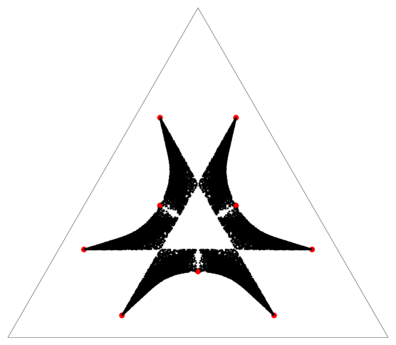
Figure 1: The spectra of 5 000 states under $\Phi^{2}$, $n=3$.

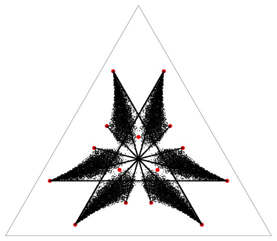
Figure 2: The spectra of 5 000 states under $\Phi^{2}$, $n=4$.

Each time we apply the map $\Phi^{1}$ the rank of the density matrix goes up one step, so $\Phi^{2}$ applied to a pure state gives a spectrum described by a point in a two-dimensional simplex. The figures show results for 5 000 pure states chosen at random according to the Fubini-Study measure, for the initial dimensions 4 and 5. The straight lines that have been added are the spectra arising from linear combinations of two number states with $|n,k\rangle$ and $|n,k^{\prime}\rangle$, $|k-k^{\prime}|>2$; for $n=4$ the image can end up in the centre, but it is highly unlikely to do so. Images of the number states are marked by red dots, with the six coherent state images outermost. The latter do majorize all other spectra since all others lie in their convex hull, typically with a large margin. Interesting patterns arise in higher dimensions, but we have not done a systematic study.

5 Fourth remark: Maximizing the Wehrl-Lieb entropy

Once it is known that the Wehrl entropy attains its minimum at the coherent states it is irresistible to ask where it attains its maximum. In the Majorana representation the problem is to choose a constellation of points on the sphere that maximizes a particular function. Simpler, but still very difficult, relatives of this problem include the Thomson problem of minimizing the electrostatic potential of $n$ electrons on a sphere and the Tammes problem of maximizing the minimal chordal distance between the electrons. The possible physical motivation behind our problem is shared by the Queens of Quantum problem to maximize the distance between a pure state and the convex hull of the coherent states Giraud .

We have not attempted a full scale optimization of the Wehrl entropy. The reason should be evident to anyone who has seen this function written out explicitly as a function of the positions of the Majorana stars Lee ; Schupp . Instead we have taken reasonable candidates for the maximum, including those known to solve the other problems, and then we have checked whether a local maximum of the Wehrl entropy results. In those cases where natural parameters appear in the constellations we have maximized over these parameters. For instance, when $n=8$ the maximum of the Thomson and the Tammes problem is given by two squares on two distinct latitude circles. This is a configuration of type $0$–$4$–$4$–$0$, and by the first remark it lies in the subspace spanned by $|8,0\rangle$, $|4,4\rangle$, and $|0,8\rangle$. We can rotate the squares relative to each other and change the difference in latitude. The Thomson, Tammes and Wehrl problems are all solved by this configuration, but the latitudes differ. In this way we have convinced ourselves that the results in the accompanying table are correct. Full details can be found elsewhere Anna .

Number	Maximum	Queen of	Thomson	Tammes
of stars	Wehrl	Quantum
3	triangle	triangle	triangle	triangle
4	tetrahedron	tetrahedron	tetrahedron	tetrahedron
5	$1$–$4$–$0$	$1$–$4$–$0$	$1$–$4$–$0$	$1$–$4$–$0$
6	octahedron	octahedron	octahedron	octahedron
7	$1$–$5$–$1$	$1$–$5$–$1$	$1$–$5$–$1$	$1$–$3$–$3$–$0$
8	$0$–$4$–$4$–$0$	looks odd	$0$–$4$–$4$–$0$	$0$–$4$–$4$–$0$
9	$0$–$3$–$3$–$3$–$0$	$0$–$3$–$3$–$3$–$0$	$0$–$3$–$3$–$3$–$0$	$0$–$3$–$3$–$3$–$0$

We would like to compare the Wehrl and Queens of Quantum problem in Hilbert spaces of dimensions as high as those number of stars for which the Thomson problem has been studied Erber However, in a note on spherical harmonics which is quite relevant here, Sylvester apologizes for treating some things sketchily because he was “very much pressed for time and within twenty-four hours of steaming back to Baltimore” Sylvester . The twenty-first century is no less pressing than was the nineteenth, and we have not been able to go further.

6 Summary

The Majorana representation of quantum states Majorana , in Hilbert spaces of dimension $N$, as consisting of constellations of $N-1$ unordered stars on a sphere Penrose , is very useful in all contexts where the group $SU(2)$ plays a dominating role. To set the stage we gave a brief discussion of how to see where we are in Hilbert space, given such a constellation. Next we gave explicit formulas for the metric and symplectic form on orbits through general angular momentum eigenstates. These orbits are interesting because they are symplectic but not Kähler, except for the coherent state orbit which goes through the highest weight states. A small observation on the Lieb-Solovej map followed. This map was introduced Solovej in order to prove that coherent states minimize the Lieb-Wehrl entropy. Given that it is irresistible to ask for those states that maximize it. We presented results on this question for dimensions $N\leq 9$. It would be interesting to see results for higher dimensions.

References

- (1) J. Schwinger, On angular momentum, in L. C. Biedenharn and H. van Dam (eds.): Quantum Theory of Angular Momentum, Academic Press 1965.
- (2) E. Majorana, Atomi orientati in campo magnetico variabile, Nuovo Cim. 9 (1932) 43.
- (3) R. Penrose, A spinor approach to general relativity, Ann. Phys. (N.Y.) 10 (1960) 171.
- (4) H. Bacry, Orbits of the rotation group on spin states, J. Math. Phys. 15 (1974) 1686.
- (5) E. H. Lieb, Proof of an entropy conjecture of Wehrl, Commun. Math. Phys. 62 (1978) 35.
- (6) E. H. Lieb and J. P. Solovej, Proof of an entropy conjecture for Bloch coherent states and its generalizations, arXiv:1208.3632.
- (7) I. Bengtsson and K Życzkowski: Geometry of Quantum States, Cambridge UP 2006.
- (8) R. Penrose, Orthogonality of general spin states, Twistor Newsletter 36 (1993) 5.
- (9) D. C. Brody and L. P. Hughston, Geometric quantum mechanics, J. Geom. Phys. 38 (2001) 19.
- (10) W. Y. Hsiang, On compact homogeneous minimal submanifolds, Proc. Nat. Acad. Sci. U.S.A. 56 (1966) 5.
- (11) A. Klyachko, Dynamic symmetry approach to entanglement, in J.-P. Gazeau et al. (eds): Proc. NATO Advanced Study Inst. on Physics and Theoretical Computer Science, IOS, Amsterdam 2007.
- (12) H. Barnum, E. Knill, G. Ortiz, and L. Viola, Generalizations of entanglement based on coherent states and convex sets, Phys. Rev. A68 (2003) 032308.
- (13) A. Sawicki, A. Huckleberry, and M. Kuś, Symplectic geometry of entanglement, Commun. Math. Phys. 305 (2011) 441.
- (14) O. Giraud, P. A. Braun, and D. Braun, Quantifying quantumness and the quest for queens of quantum, New. J. Phys. 12 (2010) 063005.
- (15) C. T. Lee, Wehrl’s entropy of spin states and Lieb’s conjecture, J. Phys. A (1988) 3749.
- (16) P. Schupp, On Lieb’s conjecture for the Wehrl entropy of Bloch coherent states, Commun. Math. Phys. 207 (1999) 481.
- (17) A. Baecklund: Maximization of the Wehrl Entropy in Finite Dimensions, MSc Thesis, KTH 2013.
- (18) T. Erber and G. M. Hockney, Complex systems: Equilibrium configurations of equal charges on a sphere ( ), Adv. Chem. Phys. 98 (1997) 495.
- (19) J. J. Sylvester, Note on Spherical Harmonics, Phil. Mag. 2 (1876) 291.