The Gamma-count distribution in the analysis of experimental underdispersed data

Abstract

Event counts are response variables with non-negative integer values representing the number of times that an event occurs within a fixed domain such as a time interval, a geographical area or a cell of a contingency table. Analysis of counts by Gaussian regression models ignores the discreteness, asymmetry and heterocedasticity and is inefficient, providing unrealistic standard errors or possibily negative predictions of the expected number of events. The Poisson regression is the standard model for count data with underlying assumptions on the generating process which may be implausible in many applications. Statisticians have long recognized the limitation of imposing equidispersion under the Poisson regression model. A typical situation is when the conditional variance exceeds the conditional mean, in which case models allowing for overdispersion are routinely used. Less reported is the case of underdispersion with fewer modelling alternatives and assessments available in the literature. One of such alternatives, the Gamma-count model, is adopted here in the analysis of an agronomic experiment designed to investigate the effect of levels of defoliation on different phenological states upon the number of cotton bolls. Results show improvements over the Poisson model and the semiparametric quasi-Poisson model in capturing the observed variability in the data. Estimating rather than assuming the underlying variance process lead to important insights into the process.

Keywords: Poisson regression, likelihood inference, gamma-count, underdispersion, quasi-Poisson, cotton.

1 Introduction

Regression models are deeply rooted in the analysis of agronomic experiments and least squares methods associated to the linear (Gaussian) model are widely adopted. On the other hand, response variable in the form of counts are not uncommon. They may represent the number of fruits produced by a tree, the number of units infected by a disease, the number of insects on a particular plant structure, among others. Counts are random variables that assume non-negative integer values, representing the number of times an event occurs within a fixed domain that can be continuous, such as an interval of time or space, or discrete, such as the evaluation of an individual or a census tract.

Gaussian regression models for count data are not efficient, typically producing inconsistent standard errors and even negative predictions for the expected number of events (?). Gaussian linear model ignores the discreteness, heterocedasticity, asymmetry and non-negativeness, inherent features of count data. Impacts on the results are greater when the sample size is small and the counts are low.

Poisson regression became the standard model for count data, in particular after the proposal of the unifying class of generalized linear models (?) and the subsequent availability of computational resources for model fitting. The Poisson distribution is an appealing option to model count data given its domain on the non negative integer numbers, moreover, it naturally allows for asymmetry and heterocedasticity that are intrinsic characteristics of this kind of data.

The assumption of variance equals to the mean (equidispersion) underlying Poisson regression models imposes practical restrictions. Parameter estimates will be inefficient, with inconsistent standard errors, and with larger error rates for hypothesis tests when the Poisson model is applied to non-equidispersed data (?; ?).

Overdispersion, with the variance greater than the mean, is largely reported in the literature and may occur due to the absence of relevant covariates, heterogeneity of sampling units, sampling levels, excess of zeros (?). An usual approach is to adopt a generalized linear mixed model (GLMM) describing the extra variability by the inclusion of a non-observed latent random variable. An interesting case is to assume a Poisson model with Gamma distributed random effects leading to a negative binomial marginal distribution for the responses. ? provides an overview of this and other alternatives.

Lesser reported are the cases of underdispersion, with variances smaller than the means. Explanatory mechanisms are more scarce and, typically, heavily dependent on the context. A possible general description can be derived by revisiting the key property of independent exponentially distributed times between events underlying the Poisson model. If inadequate, the occurrence of an event affects the probability of another one, generating over or under dispersed counts. Other continuous probability distributions with positive domain can be assumed such as Gamma (?; ?), lognormal (?) and Weibull (?). Alternative approaches includes weighting the Poisson distribution (?), the COM-Poisson distribution (?; ?) and heavy tail distributions (?).

? explores the connection between models for counts and models for durations (lifetimes) relaxing the assumption of equidispersion at the cost of an extra parameter denoted by $\alpha$. The Gamma-count model is a convenient choice assuming Gamma distributed times between events. The Poisson model becomes a particular case when the restriction $\alpha=1$ implies the durations distribution reduces to the exponential distribution. Varying values for the parameter $\alpha$ induces a flexible probability distribution for the counts, which become underdispersed for $\alpha>1$ and overdispersed for $0<\alpha<1$.

We adopt the Gamma-count model for the analysis of a cotton production agronomic experiment and compare the results against the ones obtained with Poisson and quasi-Poisson models. Firstly, standard Poisson model is not excluded since it becomes a particular case. Secondly, fitting the Gamma-count model allows for investigating whether the occurrences of bolls within a plant are independent events, an arguable assumption under the simpler Poisson model. Thirdly, descriptive analyses of the data provided a clear empirical evidence that the variance is a function of the mean with a constant of proportionality below one. We also analyze the data by a semi-parametric quasi-Poisson model as the benchmark for quantifying the observed variability in the data.

The Gamma-count regression model is not the canonical choice amongst users of applied statistics and not widely available in statistical software. For this reason, generic functions for maximum likelihood inference are available as on-line supplements. This includes key aspects related to inference upon the parameters of the Gamma-count model, such as, construction of confidence intervals, either asymptotic or based on profile likelihoods; hypothesis tests; model comparisons and prediction with corresponding confidence intervals are also included, all used throughout the data analysis.

2 Background

Poisson regression models for count data follows directly from the generalized linear model structure. Alternatively, the Poisson model can be derived by assuming independent and exponentially distributed times between events. The latter allows for the construction of alternatives for under or overdispersed data such as the Gamma-count model (?), as follows below.

Elementary probability arguments establish that the distribution of a count variable can be derived from the distribution of arrival times. Let $\tau_{k}>0$, $k\in\mathbb{N}$, denote a sequence of waiting times between the ($k-1$) and the $k^{th}$ event. Then, the arrival time of the $n^{th}$ event is

$$\vartheta_{n}=\sum_{k=1}^{n}\tau_{k},\qquad n=1,2,\ldots.$$ (1)

Let $N_{T}$ represent the total number of events within a $(0,T)$ interval. $N_{T}$ is a count variable. It follows from the definition of $N_{T}$ and $\vartheta_{n}$ that

$$N_{T}<n\quad \iff\quad\vartheta_{n}\geq T$$

$$\Pr(N_{T}<n) =\Pr(\vartheta_{n}\geq T)=1-F_{n}(T)$$

$$\Pr(N_{T}=n) =F_{n}(T)-F_{n+1}(T),$$ (2)

where $F_{n}(T)$ is the cumulative distribution function of $\vartheta_{n}$. Equation (2) allows obtaining the distribution of counts $N_{T}$ from knowledge of the distribution of arrival times $\vartheta_{n}$.

It is assumed $\tau_{k}$ are identically and independently Gamma ($G(\alpha,\beta)$) distributed with density:

$$f(\tau;\alpha,\beta)=\frac{\beta^{\alpha}}{\Gamma(\alpha)}\,\,\tau^{\alpha-1}\,\,\exp\{-\beta\tau\},\qquad\alpha,\beta\in\mathbb{R}^{+}.$$

with $\tau>0$, mean $\text{E}(\tau)=\alpha/\beta$ and variance $\text{Var}(\tau)=\alpha/\beta^{2}$. By (1), $\vartheta$ is the sum of iid Gamma random variables therefore with density $G(n\alpha,\beta)$. Let $G(n\alpha,\beta T)$ be the cumulative distribution function evaluated at $\beta T$:

$$G(n\alpha,\beta T)=F_{n}(T)=\frac{1}{\Gamma(n\alpha)}\int_{0}^{\beta T}u^{n\alpha-1}\,\,\exp\{-u\}\,\,\text{d}u.$$ (3)

The count distribution (2) for number of events within the time interval (0,$T$) is given by:

$$\Pr(N=n)=G(\alpha n,\beta T)-G(\alpha(n+1),\beta T),$$ (4)

with expected value given by:

$$\text{E}(N_{T})=\sum_{i=1}^{\infty}G(\alpha i,\beta T).$$ (5)

For $\alpha=1$, $f(\tau)$ reduces to the exponential density and (4) simplifies to the Poisson distribution.

For the Gamma-count regression model the parameters depend on a vector of individual covariates, indicated by the subscript $i$. Assuming that the period at risk is the same for all observation, $T$ can be set to unity, without loss of generality. This yields the regression

$$\text{E}(\tau_{i}|x_{i})=\frac{\alpha}{\beta}=\exp\{-x_{i}^{\top}\gamma\}.$$

Is important do emphasize that the regression is for the waiting times $\tau_{i}$ and not for the counts $N_{i}$ since $\text{E}(N_{i}|x_{i})=(\text{E}(\tau_{i}|x_{i}))^{-1}$ does not holds unless $\alpha=1$. For a given $\gamma$, $\text{E}(N_{i}|x_{i})$ is evaluated by (5).

Figure 1 illustrates the relation between the distribution of times between events and counts showing the graphics of density and hazard functions with corresponding simulated values. Gamma distributions with unity mean and different variances are shown in the first line. The second line displays the corresponding increasing, constant and decreasing hazard functions related to smaller, equal or larger variances than the mean. The middle plots correspond to the exponential distribution and its constant hazard function. The middle panel show simulated values with time intervals drawn from each of the above mentioned distributions. Vertical lines indicates fixed width intervals for which events are counted and the counts within each interval are displayed. The distribution of events is nearly regular and the counts have smaller variance in the underdispersed case. For the overdispersed case, the events are clustered with large variances for counts. Differences are evident in the resulting histograms.

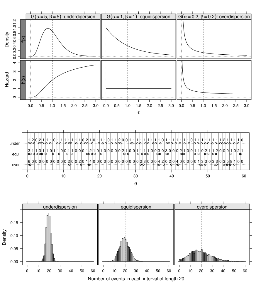
Figure 1: Comparison of different distribution of time between events. Top panel: Gamma densities and hazard functions, middle panel: simulated events and corresponding interval counts for each distribution, bottom panel: counts histograms.

For a sample if independent counts $y_{i},i=1\ldots n$, estimates $\hat{\alpha}$ and $\hat{\gamma}$ can be obtained by maximizing the log-likelihood

$$\ell(\gamma,\alpha;y,x)=\sum_{i=1}^{n}\log\left(G(y_{i}\alpha,\alpha\exp(x_{i}^{\top}\gamma))-G(y_{i}(\alpha+1),\alpha\exp(x_{i}^{\top}\gamma))\right),$$ (6)

where $\gamma$ is the vector of regression parameters describing the interval between the events, $\alpha$ is the dispersion parameter, $x_{i}$ is a vector of covariates and $G()$ is given by (3).

Parameter estimation requires numerical maximization of (6). Confidence intervals and hypotheses tests can be either based upon quadratic approximations of the likelihood function (Wald type intervals) or profile likelihoods.

For a vector $x$ of covariates values, time between events is predicted by:

$$\hat{\eta}=x^{\top}\hat{\gamma}.$$

The covariance matrix for the model parameters is:

$$V=\begin{bmatrix}V_{\alpha\alpha}\quad V_{\alpha\gamma}\\ V_{\gamma\alpha}\quad V_{\gamma\gamma}\end{bmatrix},$$

and estimated by the negative of the inverse Hessian matrix numerically obtained around the maximised log-likelihood. The prediction standard error is given by:

$$\text{se}(\hat{\eta})=\sqrt{x^{\top}V_{\gamma|\alpha}\,x},$$

where $V_{\gamma|\alpha}=V_{\gamma\gamma}-V_{\gamma\alpha}V_{\alpha\alpha}^{-1}V_{\alpha\gamma}$. For the paticular case of the Gamma-count model considered here $\alpha$ is an scalar and found to be nearly orthogonal to $\gamma$ in which case $V_{\gamma|\alpha}\approx V_{\gamma\gamma}$. Confidence intervals for the mean counts are obtained by computing (5) after transform the limits of the confidence interval on the scale of the linear predictor by the inverse link function $g^{-1}()$.

3 Data set and models

The data that motivates this paper come from a greenhouse experiment with cotton plants (Gossypium hirsutum) obtained under a completely randomized design with five replicates. The experiment aimed to assess the effects of five defoliation levels $(0,25,50,75,100\%)$ on the observed the number of bolls produced by plants at five growth stages: vegetative, flower-bud, blossom, fig and cotton boll (?). The experimental unity was a vase with two plants. The number of cotton bolls was recorded at the each culture cycle. Figure 2 (left) shows the number of cotton bolls recorded for each combination of defoliation level and growth stage. All the points in the sample means and variances dispersion diagram (right) are below the identity line, clearly suggesting the presence of underdispersion.

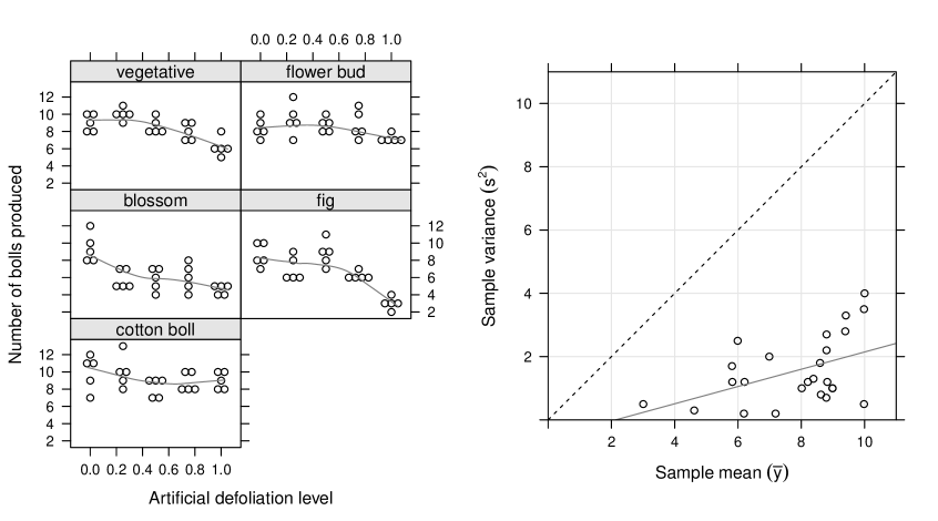
Figure 2: (left) Number of bolls produced for each artificial defoliation level and each growth stage. (right) Sample variance against the sample mean of the five replicates for each combination of defoliation level and growth stage.

The analysis and assessment of the effects of the experimental factors are based on the Gamma-count, Poisson and quasi-Poisson models, with the following structures for the log-link function $g()$:

1. Predictor 1: $g(\mu)=\gamma_{0}$;

2. Predictor 2: $g(\mu)=\gamma_{0}+\gamma_{1}\text{def}$ (first order effect of defoliation);

3. Predictor 3: $g(\mu)=\gamma_{0}+\gamma_{1}\text{def}+\gamma_{2}\text{def}^{2}$ (second order effect of defoliation);

4. Predictor 4: $g(\mu)=\gamma_{0}+\gamma_{1j}\text{def}+\gamma_{2}\text{def}^{2}$ (first order defoliation effect for each growth stage);

5. Predictor 5: $g(\mu)=\gamma_{0}+\gamma_{1j}\text{def}+\gamma_{2j}\text{def}^{2}$ (second order effect defoliation for each growth stage).

The parameter $\mu$ is the expected value of $N$ for the Poisson and quasi-Poisson models and the expected value of the latent random variable $\tau$ equivalent to time between events for the Gamma-count model.

The nested structure of the predictors allows relevant hypothesis tested by likelihood ratios. Predictor 1 contains only the intercept and is fitted simply as a baseline to assess to which extent the structured models improve the fit. Linear and quadratic effects of defoliation are added by Predictor 2 and Predictor 3, respectively. Predictor 4 and Predictor 5 allows the linear and quadratic effects of defoliation to vary between the growth stages, as indicated by the subscript $j$. The parameter $\gamma_{0}$ is not allowed to vary between the growth stage once the effect of no defoliation is the same for all growth stages.

Values of the maximized log-likelihood and the Akaike criterion are recorded for the fully parametric Poisson and Gamma-count models. The semi-parametric quasi-Poisson model is also fitted to assess whether the parametric models produce comparable results. This model is less restrictive concerning model assumptions, albeit without the inferential advantages of the fully parametric counterparts.

4 Results

Table 1 summarises the maximised log-likelihoods and likelihood ratio tests comparing the sequence of predictors for the Poisson and Gamma-count models, as well as fitting results for the quasi-Poisson. The Gamma-count model has a higher log-likelihood with the hypothesis of equidispersion ($\alpha=1$) being rejected by likelihood ratio tests, even for the predictor without covariates. Estimates of $\hat{\alpha}>1$ confirms the number of cotton bolls are underdispersed with increasing hazard functions indicating that the probability of the development of a new cotton boll increases as time progresses. This result supports the hypothesis of a regular sharing of plant resources in the distribution of the number of cotton bolls. The quasi-Poisson model also indicates underdispersion ($\phi<1$), even for the null model.

Table 1: Model fit measures and comparisons between predictors and models.

Poisson	np	$\ell$	AIC	diff np	2(diff $\ell$)	P($>\chi^{2}$)
1	1	-279.933	561.866
2	2	-272.001	548.001	1	15.864	6.805E-05
3	3	-271.354	548.709	1	1.293	2.556E-01
4	7	-258.674	531.348	4	25.360	4.258E-05
5	11	-255.803	533.606	4	5.742	2.193E-01
Gamma-count	np	$\ell$	AIC	diff np	2(diff $\ell$)	P($>\chi^{2}$)	$\hat{\alpha}$	P($>\chi^{2}$)a
1	2	-272.396	548.792				1.764	1.034E-04
2	3	-257.350	520.701	1	30.092	4.121E-08	2.266	6.198E-08
3	4	-255.981	519.962	1	2.738	9.796E-02	2.317	2.940E-08
4	8	-220.145	456.291	4	71.671	1.007E-14	4.206	1.661E-18
5	12	-208.386	440.773	4	23.518	9.976E-05	5.112	2.071E-22
Quasi-Poisson	np	deviance		diff np	diff dev	P($>F$)	$\hat{\phi}$	P($>\chi^{2}$)a
1	1	75.514					0.567	3.660E-04
2	2	59.650		1	34.214	4.235E-08	0.464	5.134E-07
3	3	58.357		1	2.810	9.630E-02	0.460	3.661E-07
4	7	32.997		4	22.768	7.676E-14	0.278	9.154E-16
5	11	27.255		4	5.956	2.241E-04	0.241	3.566E-18

np - number of parameters; $\ell$ - log-likelihood; diff np - difference in np; diff $\ell$ - difference in $\ell$; diff dev - difference in scaled deviance; ^abilateral hypothesis test of dispersion parameter equal to 1.

Unlike the others, the Poisson model does not shown significant effects under Model 5. This is attributed to the inadequate assumption of equidispersion that makes the log-likelihood among predictors less distinguishable. Descriptive levels ($p$-values) are substantially smaller for the Gamma-count and quasi-Poisson, compared with the Poisson model. In the presence of underdispersion the latter becomes conservative for hypothesis testing.

The Gamma-count and the quasi-Poisson models indicate that both, linear and quadratic effects of levels of defoliation, vary between growth stages. Results on Table 2 and Figure 3 show, for all models, no significant effects of defoliation during the floral-bud and cotton boll stages. The ratio between the estimates and the corresponding standard errors for these stages are, in absolute values, smaller than the reference value of 1.96 for a significance level of 5%. The Poisson model only detects the effect of defoliation for the blossom stage, while the Gamma-count and quasi-Poisson models indicate a significant effect of defoliation for the vegetative, blossom and fig stages.

Table 2: Parameter estimates and estimate/standard error rates for the three models.

	Poisson			quasi-Poisson			Gamma-count
Parameter	Estimate	Est/SE		Estimate	Est/SE		Estimate	Est/SE
$\gamma_{0}$	2.1896	34.5724*		2.1896	70.4205*		2.2342	79.7128*
$\gamma_{1vegetative}$	0.4369	0.8473		0.4369	1.7260		0.4122	1.8080
$\gamma_{2vegetative}$	-0.8052	-1.3790		-0.8052	-2.8089*		-0.7628	-2.9544*
$\gamma_{1bud}$	0.2897	0.5706		0.2897	1.1622		0.2744	1.2224
$\gamma_{2bud}$	-0.4879	-0.8613		-0.4879	-1.7544		-0.4642	-1.8534
$\gamma_{1blossom}$	-1.2425	-2.0581*		-1.2425	-4.1921*		-1.1821	-4.4348*
$\gamma_{2blossom}$	0.6728	0.9892		0.6728	2.0149*		0.6453	2.1486*
$\gamma_{1fig}$	0.3649	0.6449		0.3649	1.3135		0.3198	1.2797
$\gamma_{2fig}$	-1.3103	-1.9477		-1.3103	-3.9672*		-1.1990	-4.0385*
$\gamma_{1boll}$	0.0089	0.0178		0.0089	0.0362		0.0070	0.0315
$\gamma_{2boll}$	-0.0200	-0.0361		-0.0200	-0.0736		-0.0185	-0.0756
$\alpha$	-	-		-	-		5.1120	7.4228*

*indicates $|\mathrm{Est/SE}|>1.96$.

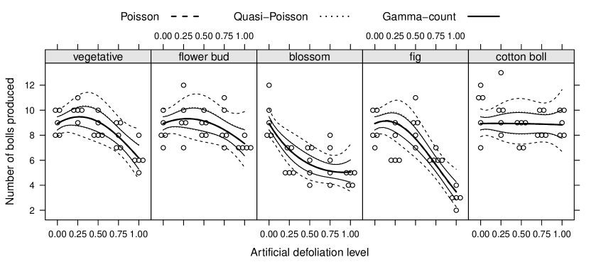
Figure 3: Dispersion diagrams of observed values and curves of predicted values and confidence intervals (95%) as functions of defoliation level for each growth stage.

Parameter estimates for the blossom stage have opposite signal when compared to the other stages. A negative and significant linear term indicates a rapid decay in the number of cotton bolls during the beginning of defoliation. The positive quadratic term indicates concave up response as seen in Figure 3 for the blossom stage. Therefore, the impact of defoliation is greater for the blossom stage and there is a tolerance up to approximately 40% of defoliation for the vegetative stage and 24% for the fig stages. Parameter estimates between models are not directly comparable once they are related to the number of events in the Poisson model and to the distribution of the time between events for the Gamma-count model.

Prediction curves for each stage are shown in Figure 3 and are indistinguishable between the three models. The confidence bands are similar between Gamma-count and quasi-Poisson models and clearly wider for the Poisson model.

Overall the Gamma-count and the quasi-Poisson model produced very similar inferential results, point and interval estimates, hypothesis tests, model comparisons and prediction bands. The semi-parametric quasi-Poisson model is expected to have a better fit to a particular data set, as there is no explicit formulation of a probability model and functional relation between mean and variance. Such flexibility comes with drawbacks. There are no likelihood measures for comparing models and submodels neither an estimated probability distribution for the counts, which could address questions of scientific interest. Table 4 provides the estimated probability distributions for the number of cotton bolls obtained under Poisson and Gamma-count models. At the level zero of defoliation, the expected value is 8.93 cotton bolls per two plants for either model, however with probability distribution more concentrated around the mean value under the Gamma-count model.

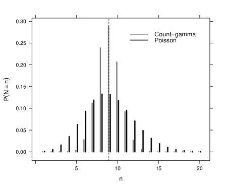
Figure 4: Estimated probabilities from Poisson and Gamma-count models for a level zero of defoliation.

In what follows we further explore aspects of the likelihood function. The profile log-likelihood for $\alpha$ is slightly skewed (left panel, Figure 5). The 95% confidence interval based on the $\chi^{2}$ distribution is $(3.89,6.59)$ while the asymptotic interval is $(3.76,6.46)$. Both have the same range (2.70) however shifted by 0.13 units. This is a small difference and the quadratic approximation of the likelihood is considered satisfactory. Although the precision of the intervals are similar, the interval based on the log-likelihood is preferred to describe the uncertainty associated with $\alpha$ since it is able to detect possible asymmetries and has limits within the $(0,\infty)$ parameter space.

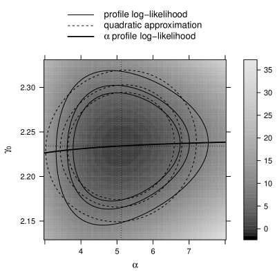
Figure 5: Profile likelihood and quadratic approximation for: (left) $\alpha$ with arrows indicating the 95% confidence intervals and (right) $(90,95,99\%)$ confidence regions for $\gamma_{0}$ and $\alpha$.

The right panel in Figure 5 shows the confidence regions for $\alpha$ and $\gamma_{0}$ obtained via profile likelihood and quadratic approximation of the likelihood. Axes of the confidence regions are nearly parallel to the Cartesian axes suggesting the parameters are nearly orthogonal. Moreover, covariances between $\hat{\alpha}$ and each of the other parameters $\hat{\gamma}$ (not shown) are nearly zero implying the inferences about one parameter are not influenced by the other parameter. The confidence regions are symmetric in the direction of $\gamma_{0}$ and the asymptotic and profile likelihood based confidence intervals are therefore coincident.

Computationally, the asymptotic confidence interval is easier to obtain since it simply requires the inversion of the Hessian matrix around the maximum of the log-likelihood function. The profile log-likelihood requires successive optimizations for a set of values of the parameter of interest. For a larger number of parameters obtaining individual intervals based on the profile the likelihoods will increase the computational burden.

5 Conclusion

The Poisson, Gamma-count and semi-parametric quasi-Poisson models were considered for the analysis of underdispersed count responses from a greenhouse experiment with cotton plants subjected to different artificial defoliation levels and growth stages.

Significance of experimental factors are the same for the Gamma-count and quasi-Poisson models whereas the Poisson model is more conservative, not identifying some experimental factors as significant. The latter have led to greater standard errors and wider prediction bands, being unable to capture information contained in the data. The analysis suggest that, in the presence of underdispersion, the standard Poisson model is inadequate and can lead to wrong conclusions about the effects of experimental factors or covariates of interest.

Results under the Gamma-count model are comparable to the semi-parametric approach which does not assume an specific probability distribution for the counts. The fully parametric approach is advantageous since it allows for likelihood based inference, deriving estimated prediction probabilities besides enabling generalizations such as specifying a regression model structure also for the dispersion parameter.

Likelihood analysis showed nearly quadratic behavior for the parameter $\alpha$ controlling the dispersion of the counts. This parameter has little influence upon point estimates of the regression parameters, being responsible for stabilizing the estimates of variances of regression parameters, which are often overestimated under the Poisson distribution.

Despite the advantages and potential for usage, the Gamma-count model is uncommon relevant addition to the suite of models to be considered for the analysis of experimental count data. The model can be easily implemented in a statistical programming language as illustrated by the supplementary material.

Possible topics for further investigation and extensions include assessment of impacts of misspecification under different levels dispersion, increase of flexibility possibly by modeling the dispersion parameter as function of covariates and the addition of random effects to account for grouped data structures such as repeated and longitudinal measures.