A frustrated spin-1 $J_{1}$–$J_{2}$ Heisenberg antiferromagnet: An anisotropic planar pyrochlore model

Abstract

The zero-temperature ground-state (GS) properties and phase diagram of a frustrated spin-1 $J_{1}$–$J_{2}$ Heisenberg model on the checkerboard square lattice are studied, using the coupled cluster method. We consider the case where the nearest-neighbour exchange bonds have strength $J_{1}>0$ and the next-nearest-neighbour exchange bonds present (viz., in the checkerboard pattern of the planar pyrochlore) have strength $J_{2}\equiv\kappa J_{1}>0$. We find significant differences from both the spin-1/2 and classical versions of the model. We find that the spin-1 model has a first phase transition at $\kappa_{c_{1}}\approx 1.00\pm 0.01$ (as does the classical model at $\kappa_{{\rm cl}}=1$) between two antiferromagnetic phases, viz., a quasiclassical Néel phase (for $\kappa<\kappa_{c_{1}}$) and one of the infinitely degenerate family of quasiclassical phases (for $\kappa>\kappa_{c_{1}}$) that exists in the classical model for $\kappa>\kappa_{{\rm cl}}$, which is now chosen by the order by disorder mechanism as (probably) the “doubled Néel” (or Néel^∗) state. By contrast, none of this family survives quantum fluctuations to form a stable GS phase in the spin-1/2 case. We also find evidence for a second quantum critical point at $\kappa_{c_{2}}\approx 2.0\pm 0.5$ in the spin-1 model, such that for $\kappa>\kappa_{c_{2}}$ the quasiclassical (Néel^∗) ordering melts and a nonclassical phase appears, which, on the basis of preliminary evidence, appears unlikely to have crossed-dimer valence-bond crystalline (CDVBC) ordering, as in the spin-1/2 case. Unlike in the spin-1/2 case, where the Néel and CDVBC phases are separated by a phase with plaquette valence-bond crystalline (PVBC) ordering, we find very preliminary evidence for such a PVBC state in the spin-1 model for all $\kappa>\kappa_{c_{2}}$.

1 Introduction

Low-dimensional spin-lattice models of magnetic systems, particularly those pertaining to frustrated Heisenberg antiferromagnets (HAFMs) with competing interactions, have been extensively studied from both the theoretical and experimental viewpoints in recent years. Although such spin-lattice models are themselves conceptually simple and easy to write down, these strongly correlated systems often exhibit rich and interesting zero-temperature ($T=0$) ground-state (GS) phase diagrams as the interaction coupling strengths are varied, due to the strong interplay between quantum fluctuations and frustration. The strength of the quantum fluctuations can itself also be tuned by a variety of methods. These include changing the spin quantum number $s$ of the particles residing on the given lattice sites, while keeping the interaction Hamiltonian unchanged. One expects that, in general, quantum fluctuations will be greatest for the case $s=\frac{1}{2}$, and that they will reduce to zero as the classical limit ($s\rightarrow\infty$) is approached.

For this reason the greatest attention has been paid to spin-1/2 magnets. Nevertheless, there has also been an upsurge of interest in spin-1 magnets in recent years. On the theoretical side, although quantum fluctuations will generally be reduced for a given model for the case $s=1$ compared with its counterpart for the case $s=\frac{1}{2}$, totally new physical effects can also sometimes enter. In one-dimensional (1D) systems these include the by now well-known existence of the gapped Haldane phase [1] with an exponential decay with separation of spin-spin correlations for $s=1$ (or, more generally, for integral values of $s$), compared to the gapless phase with a corresponding power-law decay of spin-spin correlations for $s=\frac{1}{2}$ (or, more generally, for half-odd-integral values of $s$). Also, in any number of dimensions, the possible inclusion in the $s=1$ case of such additional terms in the Hamiltonian as biquadratic exchange and single-site anisotropy, which are absent for $s=\frac{1}{2}$ systems, can lead both to novel quantum phase transitions and to novel phases with, for example, quadrupolar nematic long-range order (LRO) but with zero magnetic order parameter (taken as the average local on-site magnetization).

On the experimental side many magnetic compounds containing spin-1 ions are now established as being well described by various $s=1$ spin-lattice models. For the 1D case there are many good experimental realizations of (quasi-)linear chain systems with $s=1$. These include CsNiCl₃ [2] and Y₂BaNiO₅ [3], both with a weak easy-axis single-ion anisotropy, and CsFeBr₃ [4] with a strong easy-plane single-ion anisotropy, as well as such complex organo-metallic compounds as NENP (Ni(C₂H₈N₂)₂(NO₂)(ClO₄)) [5] with a weak planar anisotropy, and both NENC (Ni(C₂H₈N₂)₂Ni(CN₄)) [6] and DTN (NiCl₂-4SC(NH₂)₂) [7] with a strong planar anisotropy. The spin gaps seen in CsNiCl₃, Y₂BaNiO₅ and NENP are now believed to be experimental realizations of the integer-spin gap behaviour predicted by Haldane [1]. For the two-dimensional (2D) case several experimental realizations of spin-1 antiferromagnets exist. For example, K₂NiF₄ [8] provides a realization of an $s=1$ HAFM on a square lattice. Similarly, NiGa₂S₄ [9] is well described as a 2D antiferromagnet on a triangular lattice, for which the GS phase has been argued to have ferro-spin nematic order [10, 11, 12].

Of particular relevance to the present study has been the large additional impetus to the study of 2D spin-1 antiferromagnets that was provided by the discovery of superconductivity with a transition temperature $T_{c}\approx 26\,$K in the layered iron-based compound LaOFeAs, when doped by partial substitution of the oxygen atoms by fluorine atoms [13], La[O_1-xF_x]FeAs, with $x\approx$ 5–11%. That discovery was rapidly followed by finding superconductivity at even higher transition temperatures ($T_{c}\gtrsim 50\,$K) in a wide class of similarly doped quaternary oxypnictide materials. First-principles calculations [14] ensued, which showed that the original undoped parent precursor material LaOFeAs is well described by the spin-1 $J_{1}$–$J_{2}$ HAFM on a square lattice with nearest-neighbour (NN) and next-nearest-neighbour (NNN) Heisenberg exchange couplings, $J_{1}$ and $J_{2}$ respectively, with $J_{1}>0$, $J_{2}>0$, and with $J_{2}/J_{1}\approx 2$. Other authors have also reached similar conclusions (see, e.g., Ref. [15]).

The $J_{1}$–$J_{2}$ model on a square lattice has itself received huge theoretical attention over the last 25 or so years, since it provides an archetypal model of a strongly correlated and highly frustrated spin-lattice system. Most attention has naturally been devoted to the spin-1/2 case (see, e.g., Refs. [16, 17, 18, 19, 20, 21, 22, 23, 24, 25, 26, 27, 28, 29, 30, 31, 32, 33, 34, 35, 36, 37, 38, 39, 40, 41, 42, 43, 44, 45, 46, 47, 48] and references therein). The consensual view for this model now is that its ($T=0$) GS phase diagram exhibits two phases with quasiclassical LRO, both with antiferromagnetic (AFM) order, namely, a Néel-ordered phase (with a wavevector ${\mathbf{Q}}=(\pi,\pi)$) at small values of the frustration parameter ($J_{2}/J_{1}\lesssim 0.4$) and a collinear stripe-ordered phase (with a wavevector ${\mathbf{Q}}=(\pi,0)$ or ${\mathbf{Q}}=(0,\pi)$) at large values ($J_{2}/J_{1}\gtrsim 0.6)$. These two magnetically ordered phases are separated by an intermediate quantum paramagnetic (QP) phase without magnetic LRO for $0.4\lesssim J_{2}/J_{1}\lesssim 0.6$. What makes the system of continuing interest is that the nature of the intermediate QP phase and the order and nature of the two phase transitions bounding it are still not fully resolved and understood.

The classical ($s\rightarrow\infty$) version of the $J_{1}$–$J_{2}$ model on the square lattice (with a number $N\rightarrow\infty$ of spins) exhibits a unique GS Néel-ordered AFM phase for $J_{2}/J_{1}<\frac{1}{2}$, with an energy per spin $E^{\rm cl}/N=-2s^{2}(J_{1}-J_{2})$, but has an infinitely degenerate set of GS phases for $J_{2}/J_{1}>\frac{1}{2}$, all with $E^{\rm cl}/N=-2s^{2}J_{2}$. The latter set comprises two interpenetrating Néel-ordered $\sqrt{2}\times\sqrt{2}$ square lattices, with the relative ordering angle between them completely arbitrary. Quantum fluctuations then act, via the well known order by disorder mechanism [49, 50], to lift this (accidental) degeneracy in the quasiclassical ($s\gg 1$) limit where one works to leading order in $1/s$, in favour of collinear ordering, which leads to the two (row or column) stripe-ordered states, with wavevectors ${\mathbf{Q}}=(0,\pi)$ and ${\mathbf{Q}}=(\pi,0)$, discussed above.

This feature of macroscopic classical GS degeneracy in any spin-lattice model always makes such models of particular theoretical interest since they are, a priori, prime candidates for exhibiting novel quantum GS phases. It also makes them particularly susceptible to small perturbations in the form, for example, of additional spin-orbit interactions, spin-lattice couplings, neglected exchange terms, and anisotropies in the exchange interactions. Hence, considerable attention has also been placed on various such mechanisms, or extra parameters that can be included, to extend the $J_{1}$–$J_{2}$ model on the square lattice, apart from changing the spin quantum number, both to learn more about the model itself and to enquire how robust are its various properties against any such perturbations.

Naturally, for the purpose of making such detailed comparisons, it is important to use an accurate theoretical technique with controlled approximation hierarchies. One such is the coupled cluster method (CCM) [51, 52, 53, 54] that we shall employ here, and which we discuss in more detail in Sec. 3. The CCM has been very successfully applied over the last 20 or more years to a wide variety of quantum spin-lattice systems (see, e.g., Refs. [28, 37, 38, 41, 43, 53, 54, 55, 56, 57, 58, 59, 60, 61, 62, 63, 64, 65, 66, 67, 68, 69, 70, 71, 72, 73, 74, 75, 76, 77, 78, 79, 80, 81, 82, 83, 84, 85, 86, 87, 88] and references cited therein). These include applications both to the square-lattice $J_{1}$–$J_{2}$ model itself [28, 38, 43, 73] as well as to various extensions and refinements of it along the lines discussed above.

Such extensions include, inter alia: (a) the $J_{1}$–$J_{2}$–$J_{\perp}$ model of a stacked square lattice [37], in which a number of 2D $J_{1}$–$J_{2}$ square-lattice layers are coupled via a NN inter-layer exchange interaction of strength $J_{\perp}$; (b) putting a square-plaquette structure on the model [43] by having differing inter- and intra-plaquette NN couplings; (c) the corresponding $J_{1}$–$J_{2}$–$J_{3}$ model [41], which includes next-next-nearest-neighbour Heisenberg couplings of strength $J_{3}$; (d) the $J_{1}$–$J_{1}^{\prime}$–$J_{2}$ model [68], in which a spatial anisotropy between NN bonds along the two perpendicular square-lattice directions is introduced; and (e) the $J_{1}^{XXZ}$–$J_{2}^{XXZ}$ model [67], in which an $XXZ$-type anisotropy is introduced on both the NN and NNN Heisenberg exchange bonds. The corresponding $s=1$ cases have also been studied within the CCM framework for the latter two cases of the $J_{1}$–$J_{1}^{\prime}$–$J_{2}$ model [69] and the $J_{1}^{XXZ}$–$J_{2}^{XXZ}$ model [70] on the square lattice.

Of particular importance for, and relevance to, the present paper, we note that the CCM has also been applied to study the ($T=0$) GS phase diagrams of several members of the so-called half-depleted spin-1/2 $J_{1}$–$J_{2}$ models on the square lattice, all of which share the feature that half of the $J_{2}$ bonds of the original model are removed. They differ only in the arrangements of the remaining $J_{2}$ bonds. When each basic square plaquette (formed from 4 NN $J_{1}$ bonds) has a single $J_{2}$ bond, they include the three cases of: (a) the interpolating square-triangle model [72], in which the $J_{2}$ bonds have the same orientation in each square plaquette; (b) the Union Jack model [74], in which the $J_{2}$ bonds have alternating orientations on neighbouring square plaquettes; and (c) the chevron-decorated square-lattice model [87], in which the $J_{2}$ bonds alternate in orientation in one direction (say, along rows), but are parallel to each other in the perpendicular direction (say, along columns).

The corresponding $s=\frac{1}{2}$ model on the checkerboard lattice, in which alternating basic square plaquettes have either both or zero $J_{2}$ bonds present, has also been studied within the CCM [83]. Furthermore, CCM studies have also been carried out for $s\geq 1$ cases of both the interpolating square-triangle lattice model [79] and the Union Jack model [76], which both show interesting differences to their $s=\frac{1}{2}$ counterparts. The aim of the present work is to perform a similar CCM analysis of the $s=1$ version of the $J_{1}$–$J_{2}$ model on the checkerboard lattice, and to compare it with its $s=\frac{1}{2}$ counterpart studied previously by us [83].

The $J_{1}$–$J_{2}$ model on the checkerboard lattice, shown schematically in Fig. 1, is also known as the anisotropic planar pyrochlore (APP) model (or, sometimes, the crossed chain model). It may be regarded as a 2D analogue of a three-dimensional (3D) anisotropic pyrochlore model of corner-sharing tetrahedra. The model itself, as we elaborate in Sec. 2, falls into the same interesting class as the full $J_{1}$–$J_{2}$ model on the square lattice, demonstrating macroscopic classical GS degeneracy above a certain critical value of the anisotropy parameter, $\kappa\equiv J_{2}/J_{1}$. For that reason the ($T=0$) GS phase diagram of the $s=\frac{1}{2}$ version of the model has been much studied earlier by many authors [83, 89, 90, 91, 92, 93, 94, 95, 96, 97, 98, 99, 100, 101, 102, 103, 104, 105, 106]. More recently, on the basis of our CCM results for this model [83], a more accurate and, hopefully, more consensual description of its GS phase structure is emerging. The time now seems ripe, therefore, to compare and contrast the model with its $s=1$ counterpart, which we study here.

In Sec. 2 the model itself is discussed, before we give a brief description of the CCM formalism in Sec. 3. Our main results are then presented in Sec. 4, and we end with a discussion and summary in Sec. 5.

2 The model

The Hamiltonian of the $J_{1}$–$J_{2}$ model on the checkerboard lattice is given by

$$H=J_{1}\sum_{\langle i,j\rangle}\mathbf{s}_{i}\cdot\mathbf{s}_{j}+J_{2}\sum_{\langle\langle i,k\rangle\rangle^{\prime}}\mathbf{s}_{i}\cdot\mathbf{s}_{k}\,,$$ (1)

where the indices runs over all sites of a 2D square lattice, such that the sum over $\langle i,j\rangle$ counts every NN pair (once and once only) and the sum over $\langle\langle i,k\rangle\rangle^{\prime}$ counts each NNN pair in the checkerboard pattern (once and once only) shown in Fig. 1, such that alternate basic square plaquettes have either two diagonal bonds or none. Each site $i$ of the lattice now carries a particle with spin $s=1$ described by a spin operator ${\bf s}_{i}=(s_{i}^{x},s_{i}^{y},s_{i}^{z})$.

 

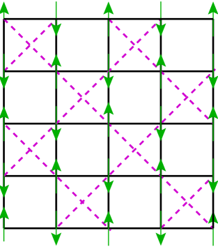
(a) Néel

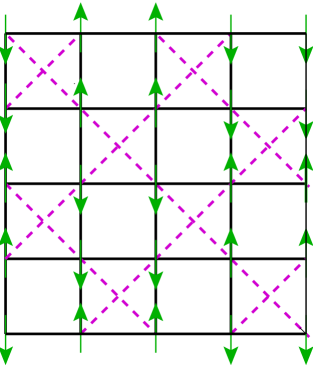
(b) Néel^∗

Figure 1: The $J_{1}$–$J_{2}$ checkerboard model, showing (a) the Néel state, and (b) one of the two Néel^∗ states. The NN $J_{1}$ bonds are shown as solid (black) lines and the NNN (i.e., also NN) $J_{2}$ bonds are shown as dashed (magenta) lines. The arrows represent the orientations of the spins on each lattice site for each of the three states shown.

The lattice and exchange bonds of the anisotropic planar pyrochlore model are thus shown in Fig. 1, from which one sees clearly how it may alternatively be construed as comprising crossed (diagonal) sets of chains, along which the intrachain exchange coupling constant is $J_{2}$, coupled by both vertical and horizontal interchain exchange bonds of strength $J_{1}$. Both bonds here are assumed to be AFM in nature (i.e., $J_{1}>0$ and $J_{2}>0$) and hence to act to frustrate one another. Clearly, the model interpolates smoothly between the HAFM on the square lattice (when $\kappa\equiv J_{2}/J_{1}=0$) and decoupled 1D isotropic HAFM chains (when $\kappa\rightarrow\infty$). When $\kappa=1$, in between these limiting cases, we have the isotropic HAFM on the checkerboard lattice, alias the isotropic planar pyrochlore. With no loss of generality, henceforth we choose $J_{1}\equiv 1$ to set the overall energy scale.

Classically (i.e., when $s\rightarrow\infty$) the model has a single ($T=0$) GS phase transition at $\kappa=\kappa_{{\rm cl}}=1$. For $\kappa<1$ the GS phase is the Néel state illustrated in Fig. 1(a), for which the ordering along the diagonal chains is hence ferromagnetic (FM) in nature. The GS energy per spin of this classical Néel state is thus $E^{{\rm cl}}/N=s^{2}(-2J_{1}+J_{2}$). For $\kappa>1$ the corresponding GS phase is now infinitely degenerate. It comprises a set of collinear states in which every checkerboard diagonal chain of sites connected by $J_{2}$ bonds has Néel AFM ordering, but where each chain can slide along its own length without changing the overall energy. In other words, the infinite degeneracy in this set is such that the spins along any one row or column can be arbitrarily assigned. All such states then have the same classical energy per spin, $E^{{\rm cl}}/N=-s^{2}J_{2}$, independent of the value of $J_{1}$. Among this infinite family of states is the so-called Néel^∗ state shown in Fig. 1(b), which has pairwise or doubled AFM ordering of the type $\cdots\uparrow\uparrow\downarrow\downarrow\uparrow\uparrow\downarrow\downarrow\cdots$, along every row and column. Thus, the single spin $\uparrow$ or $\downarrow$ of the Néel state is replaced by the two-site unit $\uparrow\uparrow$ or $\downarrow\downarrow$ in the Néel^∗ state. The Néel^∗ state retains a double degeneracy. This can easily be seen, for example, from Fig. 1(b), where the Néel^∗ state exhibits two forms of empty plaquettes (namely, those with four parallel spins and those with two pairs of antiparallel spins), the roles of which can be interchanged.

In our previous [83] CCM analysis of the $s=\frac{1}{2}$ version of the model we found a GS phase diagram with marked differences to its classical ($s\rightarrow\infty$) counterpart. Although the quasiclassical state with Néel AFM ordering remains the GS phase for low enough values of $\kappa$ (viz., $\kappa<\kappa_{c}^{1}\approx 0.80\pm 0.01$), we found that none of the infinitely degenerate set of AFM states in the classical model (which form the GS phase in that case for $\kappa>1$) can survive the quantum fluctuations present in the $s=\frac{1}{2}$ case to form a stable GS phase. We found instead two different forms of valence-bond crystalline (VBC) ordering for $\kappa>\kappa_{c}^{1}$. Firstly, in the region $\kappa_{c}^{1}<\kappa<\kappa_{c}^{2}\approx 1.22\pm 0.02$ we found the stable GS phase to exhibit plaquette VBC (PVBC) order, while for all $\kappa>\kappa_{c}^{2}$ the ordering changes to a crossed-dimer VBC (CDVBC) variety. We found that both transitions are probably direct ones, although, as usual, we could not entirely rule out very narrow coexistence regions confined, respectively, to $0.79\lesssim\kappa\lesssim 0.81$ and $1.20\lesssim\kappa\lesssim 1.22$.

In view of our earlier discussion in Sec. 1, it is now of great interest to perform a comparable analysis of the $s=1$ version of the model, the results of which we present in Sec. 4 after a brief discussion of the CCM formalism used to obtain them.

3 The coupled cluster method

Since the CCM is well documented elsewhere (see, e.g., Refs. [51, 52, 53, 54]) we give only a brief outline here. We note that it is particularly well suited for the study of such highly frustrated magnets as we consider here, for which alternative methods, such as quantum Monte Carlo (QMC) or exact diagonalization (ED) techniques, run into severe problems. Thus, QMC methods suffer in such cases from the infamous “minus-sign problem,” while ED methods are often restricted to too small lattices to be able to sample with sufficient accuracy the details of the often very subtle ordering that is present, even when state-of-the-art calculations are performed with the largest computational resources available. While both QMC and ED calculations are performed on lattices with a finite number $N$ of spins, and hence require finite-size scaling to obtain the $N\rightarrow\infty$ limit required, the CCM, as we described below, is a size-extensive method that automatically works in the (infinite-lattice) thermodynamic limit from the outset, at every level of approximation. Since such approximations, as we will see below, can be defined in rigorous hierarchical schemes, the only final extrapolation needed is to the (exact) limit in any such scheme. Furthermore, at the highest levels of approximation feasible with available computational resources, results for physical quantities are often already well converged, as our specific results in Sec. 4 will show.

The CCM starts with the choice of a suitable model state (or reference state), $|\Phi\rangle$, on top of which the quantum correlations present in the exact GS phase under study can be systematically incorporated later, as we described below. For the present model obvious choices are the Néel and Néel^∗ states shown in Fig. 1. At the quasiclassical level we expect these might prove good candidate CCM model states for the regions $\kappa\lesssim 1$ and $\kappa\gtrsim 1$, respectively. Of course, for the latter regime there is an infinite family of classically degenerate states from which to choose. We note, in this context, however, that at the $O(1/s)$ level in a quasiclassical expansion in powers of $1/s$, a fourfold set of states is selected [97] by the order by disorder mechanism [49, 50] to lie lowest in energy. These include the (doubly degenerate) Néel^∗ states as well as the two (row and column) striped AFM states, in which alternating rows or columns have spins aligned $\uparrow$ or $\downarrow$.

Once a model state $|\Phi\rangle$ is chosen, the exact GS ket- and bra-state wave functions that satisfy the corresponding Schrödinger equations,

$$H|\Psi\rangle=E|\Psi\rangle\,;\quad\langle\tilde{\Psi}|H=E\langle\tilde{\Psi}|\,,\quad$$ (2)

are parametrized as

$$|\Psi\rangle={\rm e}^{S}|\Phi\rangle\,;\quad\langle\tilde{\Psi}|=\langle\Phi|\tilde{S}{\rm e}^{-S}\,,$$ (3)

where we use the intermediate normalization scheme for $|\Psi\rangle$, such that $\langle\Phi|\Psi\rangle=\langle\Phi|\Phi\rangle\equiv 1$, and then for $\langle\tilde{\Psi}|$ choose its normalization such that $\langle\tilde{\Psi}|\Psi\rangle=1$. The correlation operators $S$ and $\tilde{S}$ are decomposed in terms of exact sets of multiparticle, multiconfigurational creation and destruction operators, $C^{+}_{I}$ and $C^{-}_{I}\equiv(C^{+}_{I})^{\dagger}$, respectively, as

$$S=\sum_{I\neq 0}{\cal S}_{I}C^{+}_{I}\,;\quad\tilde{S}=1+\sum_{I\neq 0}\tilde{{\cal S}}_{I}C^{-}_{I}\,,$$ (4)

where $C^{+}_{0}\equiv 1$, the identity operator, and $I$ is a set index describing a complete set of single-particle configurations for all of the particles. The reference state $|\Phi\rangle$ thus acts as a fiducial (or cyclic) vector, or generalized vacuum state, with respect to the complete set of creation operators $\{C^{+}_{I}\}$, which are hence required to satisfy the conditions $\langle\Phi|C^{+}_{I}=0=C^{-}_{I}|\Phi\rangle\,,\forall I\neq 0$.

In order to consider each site on the spin lattice to be equivalent to all others, whatever the choice of state $|\Phi\rangle$, it is convenient to form a passive rotation of each spin so that in its own local spin-coordinate frame it points in the downward, (i.e., negative $z$) direction. Clearly, such choices of local spin-coordinate frames leave the basic SU(2) spin commutation relations unchanged, but have the nice effect that the $C^{+}_{I}$ operators can be expressed as products of single-spin raising operators $s^{+}_{k}\equiv s^{x}_{k}+is^{y}_{k}$, such that $C^{+}_{I}\equiv s^{+}_{k_{1}}s^{+}_{k_{2}}\cdots s^{+}_{k_{n}};\;n=1,2,\cdots,2sN$.

The complete set of multiparticle correlation coefficients $\{{\cal S}_{I},{\tilde{\cal S}}_{I}\}$ may now be evaluated by extremizing the energy expectation value $\bar{H}\equiv\langle\tilde{\Psi}|H|\Psi\rangle=\langle\Phi|{\tilde{S}}{\rm e}^{-S}H{\rm e}^{S}|\Phi\rangle$, with respect to each of them, $\forall I\neq 0$. Variation with respect to each coefficient ${\tilde{\cal S}}_{I}$ yields the coupled set of nonlinear equations,

$$\langle\Phi|C^{-}_{I}{\rm e}^{-S}H{\rm e}^{S}|\Phi\rangle=0\,,\quad\forall I\neq 0\,,$$ (5)

for the coefficients $\{{\cal S}_{I}\}$, while variation with respect to each coefficient ${\cal S}_{I}$ yields the corresponding set of linear equations,

$$\langle\Phi|\tilde{S}({\rm e}^{-S}H{\rm e}^{S}-E)C^{+}_{I}|\Phi\rangle=0\,,\quad\forall I\neq 0\,,$$ (6)

for the coefficients $\{{\tilde{\cal S}}_{I}\}$, once the coefficients $\{{\cal S}_{I}\}$ have been calculated from Eq. (5), and where in Eq. (6) we have used Eqs. (3) and (4) to introduce the GS energy $E$.

Up till now everything has been exact. In practice, of course, approximations need to be made, and these are made within the CCM by restricting the set of indices $\{I\}$ retained in the expansions of Eq. (4) for the otherwise exact correlation operators $S$ and $\tilde{S}$. Some specific such hierarchical scheme are described below. It is important to realize, however, that no further approximations are made. In particular, the method is guaranteed by the use of the exponential parametrizations in Eq. (3) to be size-extensive at every level of truncation, and hence we work from the outset in the $N\rightarrow\infty$ limit. Similarly, the important Hellmann-Feynman theorem is similarly exactly obeyed at every level of truncation. Lastly, when the similarity-transformed Hamiltonian ${\rm e}^{-S}H{\rm e}^{S}$ in Eqs. (5) and (6) is expanded in powers of $S$ using the well-known nested commutator expansion, the fact that $S$ contains only spin-raising operators guarantees that the otherwise infinite expansion actually terminates at a finite order, so that no further approximations are needed.

Once an approximation has been chosen and the retained coefficients $\{{\cal S}_{I},{\tilde{\cal S}}_{I}\}$ calculated from Eqs. (5) and (6), any GS quantity can, in principle, be calculated. For example, the GS energy $E$ can be calculated in terms of the coefficients $\{{\cal S}_{I}\}$ alone, as $E=\langle\Phi|{\rm e}^{-S}H{\rm e}^{S}|\Phi\rangle$, while the average on-site GS magnetization (or magnetic order parameter) $M$ needs both sets $\{{\cal S}_{I}\}$ and $\{{\tilde{\cal S}}_{I}\}$ for its evaluation as $M=-\frac{1}{N}\langle\Phi|\tilde{S}{\rm e}^{-S}\sum^{N}_{k=1}s^{z}_{k}{\rm e}^{S}|\Phi\rangle$, in terms of the rotated local spin-coordinate frames defined above.

In our previous work for the $s=\frac{1}{2}$ model [83] we employed the well-known and well-tested localized LSUB$m$ CCM approximation scheme (see Refs. [53, 54]). At the $m$th level of approximation it includes all spin clusters described by multispin configurations in the index set $\{I\}$ that may be defined over any possible lattice animal (or polyomino) of size $m$ on the lattice. Such a lattice animal is defined in the usual graph-theoretic sense to be a configured set of contiguous sites on the lattice, in which every site in the configuration is adjacent (in the NN sense) to at least one other site. Clearly, as $m\rightarrow\infty$ the LSUB$m$ approximation becomes exact. The definition of contiguity employed above depends itself on the choice of “geometry” of the lattice, i.e., on the definition of what is meant by a NN pair. Just as in our previous treatment [83] of the $s=\frac{1}{2}$ version of the present $s=1$ model, we assume the fundamental checkerboard geometry to define the retained configurations, in which pairs of sites connected either by a $J_{1}$ bond or by a $J_{2}$ bond are defined to be contiguous (or as NN pairs for the sake of defining a lattice animal of a given size). Although the number of retained configurations at a given $m$th level of approximation is larger in the checkerboard geometry than in the corresponding square-lattice geometry (for which pairs connected by $J_{2}$ bonds would be NNN pairs), the advantage is that the former choice retains many of the symmetries of the checkerboard-lattice model at all levels of approximation that would be lost in the latter choice.

At a given $m$th level of LSUB$m$ approximation (with any fixed choice of underlying geometry to define contiguity) the number, $N_{f}$, of such distinct (i.e., under the symmetries of the lattice and specified model state) fundamental spin configurations is lowest for $s=\frac{1}{2}$ and rises steeply as $s$ increases. This is because each downward-pointing (in the rotated local frame) spin on each site $k$ may be operated upon by the spin-raising operator $s^{+}_{k}$ up to 2$s$ times. Thus each site index $k_{i}$ in the operators $C^{+}_{I}\equiv s^{+}_{k_{1}}s^{+}_{k_{2}}\cdots s^{+}_{k_{n}}$ may be repeated up to a maximum of 2$s$ times. For such $s>\frac{1}{2}$ cases, where individual indices may be repeated, an alternative, so-called SUB$n$–$m$, CCM scheme has been used. This scheme doubly restricts the configured clusters included to contain no more than $n$ spin-flips (where each spin-flip requires the action of an $s^{+}_{k}$ operator acting once) spanning a range of no more than $m$ contiguous sites on the lattice. We then set $m=n$ and employ here the SUB$n$–$n$ scheme. Clearly, the LSUB$m$ scheme is equivalent to the SUB$n$–$m$ scheme when $n=2sm$ for particles of spin $s$. For the $s=\frac{1}{2}$ case only, LSUB$m$ $=$ SUB$m$–$m$, whereas for the $s=1$ case LSUB$m\equiv$ SUB2$m$–$m$. We note that the corresponding numbers, $N_{f}$, of fundamental configurations at a given SUB$n$–$n$ level are higher for the $s=1$ case than for the $s=\frac{1}{2}$ case. Thus, whereas for the $s=\frac{1}{2}$ case we were able to perform LSUB$m$ calculations with $m\leq 10$ previously [83], with similar supercomputer resources available we are now only able to perform SUB$n$–$n$ calculations for the $s=1$ case that are restricted to $n\leq 8$. As before [83] we similarly use massively parallel computation [107] to derive and solve the corresponding coupled sets of CCM equations (5) and (6).

As a last step we need to extrapolate the approximate SUB$n$–$n$ results thus obtained to the exact $n\rightarrow\infty$ limit. Just as for the $s=\frac{1}{2}$ version of the model [83] we use for the $s=1$ version the very well tested and very robust approximation scheme,

$$\frac{E(n)}{N}=a_{0}+a_{1}n^{-2}+a_{2}n^{-4}\,,$$ (7)

for the GS energy per spin [37, 38, 41, 61, 62, 63, 65, 66, 67, 68, 69, 70, 72, 73, 74, 75, 76, 77, 78, 79, 80, 81, 82, 83, 84, 85, 86, 87]. Not surprisingly, the GS expectation values of other physical observables both tend to converge more slowly than the GS energy, and with leading exponents that can also depend on the model and regime under study. More specifically, the amount of frustration present can then often determine the scaling.

For example, for most systems with no or moderate amounts of frustration present, the magnetic order parameter $M$ has been widely found [62, 61, 63, 65, 72, 74, 75, 76] to obey a scaling law with leading power $1/n$ (rather than with $1/n^{2}$ as for the GS energy). In such cases an extrapolation scheme of the form

$$M(n)=b_{0}+b_{1}n^{-1}+b_{2}n^{-2}\,,$$ (8)

works well. However, for systems which are close to a quantum critical point (QCP) or for which the magnetic order parameter for the phase being studied is zero or close to zero, the extrapolation scheme of Eq. (8) tends always to overestimate the (extrapolated value of the) order parameter and hence also to predict a somewhat too large value for the critical strength of the frustrating interaction that drives the transition under study. In such cases much evidence has by now been accumulated that a scaling law with leading power $1/n^{1/2}$ works much better to fit the SUB$n$–$n$ data. In such cases we then use the alternative well-studied extrapolation scheme  [37, 38, 41, 67, 68, 69, 70, 73, 77, 78, 79, 80, 81, 82, 83, 84, 85, 86, 87],

$$M(n)=c_{0}+c_{1}n^{-1/2}+c_{2}n^{-3/2}\,.$$ (9)

For any physical observable $P$ of any spin-lattice model being studied by the CCM, we may obviously always test for the correct scaling by first fitting the SUB$n$–$n$ results to a form

$$P(n)=p_{0}+p_{1}n^{-\nu}\,,$$ (10)

where the leading exponent $\nu$ is also a fitting parameter. For the GS energy $E$ such fits generally yield a fitted value of $\nu$ very close to 2 for a wide variety of both unfrustrated and (even highly) frustrated systems in different phases, as is also the case here. Such a preliminary fit then justifies the use of Eq. (7) to find the extrapolated value of $E/N$. A similar preliminary analysis for the order parameter $M$ can be done in specific cases to justify the use of either Eq. (8) or Eq. (9) to find the extrapolated value of $M$.

For the model at hand we have performed extrapolations for all of the physical observables calculated using each of the SUB$n$–$n$ data sets with $n=\{2,4,6,8\}$ and $n=\{4,6,8\}$ (and also $n=\{2,4,6\}$, even though this set is clearly not a preferred set), as a further test of the robustness of the schemes used. In each case we find very similar results for the extrapolated values, thereby lending credence to the extrapolation schemes used to find them.

4 Results

We now present our CCM results for the spin-1 $J_{1}$–$J_{2}$ model on the checkerboard lattice, using both the Néel and Néel^∗ states shown in Fig. 1 as model states, and employing the SUB$n$–$n$ truncation scheme with $n\leq 8$. Figure 2 firstly shows the results for the GS energy per spin, $E/N$. We display both “raw” SUB$n$–$n$ results and extrapolations to the $n\rightarrow\infty$ limit based on the use of Eq. (7) with either the data set $n=\{2,4,6,8\}$ or $n=\{4,6,8\}$.

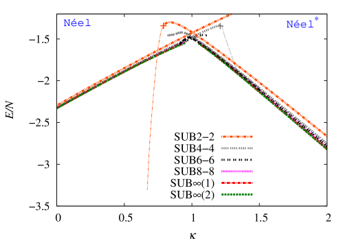
Figure 2: CCM results for the GS energy per spin, $E/N$, as a function of the frustration parameter, $\kappa\equiv J_{2}/J_{1}$, for the spin-1 $J_{1}$–$J_{2}$ Heisenberg antiferromagnet (with $J_{1}\equiv 1$) on the checkerboard lattice. The results for the SUB$n$–$n$ approximations with $n=\{2,4,6,8\}$ based on the Néel state (left curves) and Néel^∗ state (right curves) as the respective CCM model state are shown, together with the corresponding SUB$\infty(k)$ extrapolations obtained from using Eq. (7) together with the respective SUB$n$–$n$ data sets: $k=1$, $n=\{2,4,6,8\}$; and $k=2$, $n=\{4,6,8\}$. All SUB$n$–$n$ solutions are shown out to their respective (approximately determined) mathematical termination points; and the plus ($+$) symbols mark those points where the corresponding solutions have vanishing order parameter $M=0$ (and see Fig. 3(a)). Those portions of the curves beyond the plus ($+$) symbols, shown with thinner curves, indicate unphysical regions, where $M<0$ for these approximations (and see text for further details).

The first thing to notice is how well converged the results are for both sets of results based on the Néel state (left curves) and Néel^∗ state (right curves). Secondly, we note that, exactly as for the $s=\frac{1}{2}$ case studied previously [83], both sets of curves display termination points, at particular values of $\kappa$, namely, an upper one for the Néel curves and a lower one for the Néel^∗ curves, beyond which no real solutions exist. The termination points themselves depend on the particular SUB$n$–$n$ approximation used. What is generally observed is that as the truncation index $n$ is increased the range of values of the frustration parameter $\kappa$ over which the corresponding SUB$n$–$n$ approximations have real solutions decreases, as may clearly be seen from Fig. 2. Such CCM termination points are by now well understood [54, 74]. Indeed, they provide a clear first signal of the corresponding QCPs that exist in the system under study. However, we note that it is computationally expensive to obtain the actual termination point with great accuracy, since the CCM SUB$n$–$n$ solutions require increasingly more computing power the nearer one approaches a termination point. Thus, particularly for the higher values of the truncation index $n$, it is almost certain that real solutions exist for slightly larger ranges of $\kappa$ than those shown.

In the vicinity of any such mathematical CCM SUB$n$–$n$ (or LSUB$m$) solution termination points it is commonly found, as is the case here too as we shall see explicitly below, that the corresponding solutions themselves become unphysical in the sense that the respective values of the magnetic order parameter (namely, the local on-site magnetization, $M$) become negative. These values where $M$ changes sign in this way, determined as discussed below, are denoted by plus sign ($+$) symbols in Fig. 2, and the unphysical regions beyond them, out to the mathematical termination points, where $M<0$ are shown by thinner curves than the corresponding physical regions where $M>0$ that are marked by thicker curves.

We note from Fig. 2 that the corresponding SUB$n$–$n$ curves for $E/N$ based on the Néel and the Néel^∗ states, intersect one another for the same level $n$ of truncation, at least for $n\leq 6$. It is almost certain that this is true too for the $n=8$ curves, although it is computationally expensive to find the solutions in this region, as indicated above. Furthermore, we note that as the truncation index $n$ increases, the angle of intersection of the corresponding SUB$n$–$n$ Néel and Néel^∗ curves decreases. Indeed, the corresponding extrapolated curves seem highly likely to join smoothly. Thus, there are clear preliminary indications that the first-order phase transition at $\kappa_{{\rm cl}}=1$ in the classical ($s\rightarrow\infty$) version of the model might even become a continuous second-order transition in its $s=1$ counterpart. The energy crossing point of the Néel and Néel^∗ results for the $s=1$ model is estimated to be $\kappa_{c_{1}}\approx 1.00\pm 0.01$ based on our CCM SUB$n$–$n$ results for $n=\{2,4,6\}$ and a corresponding extrapolation based on these results.

Thus, based on the energy results alone, the $s=1$ model seems to share this transition point at which Néel order melts with its classical ($s\rightarrow\infty$) counterpart. Nevertheless, there are first indictions that the classical first-order transition at $\kappa_{{\rm cl}}=1$ might become of second-order type for the $s=1$ model. By contrast, as was shown earlier [83], in the $s=\frac{1}{2}$ model Néel order melts at a lower QCP, namely $\kappa_{c}^{1}\approx 0.80\pm 0.01$, at which point it gives way not to the quasiclassical Néel^∗ state (or any other of the infinitely degenerate family of classical states) but to a PVBC-ordered state.

In order to investigate the overall level of accuracy of our results it is worthwhile to examine the two special limiting cases of $\kappa=0$ (square-lattice HAFM) and $\kappa\rightarrow\infty$ (decoupled 1D HAFM chains). Thus, firstly, based on the Néel state as the CCM model state, our extrapolated results for the GS energy per spin for the spin-1 square-lattice HAFM are $E(\kappa=0)/N\approx-2.3287$ based on the SUB$n$–$n$ results using the data set $n=\{4,6,8\}$ and $E(\kappa=0)/N\approx-2.3292$ using the corresponding data set $n=\{2,4,6,8\}$. These are in very good agreement with the alternative results $E(\kappa=0)/N\approx-2.3282$ based on third-order spin-wave theory (SWT-3) [108] and $E(\kappa=0)/N=-2.3279(2)$ based on a linked-cluster series expansion (SE) technique [109]. Our results are also in essentially exact agreement for this $\kappa=0$ case with previous CCM estimates that are similar limiting cases of spin-1 $J_{1}$–$J_{2}$ models on the Union Jack lattice [76] and an anisotropic triangular lattice [79], both of which reduce to the square-lattice HAFM when $J_{2}=0$. Secondly, based on the Néel^∗ state as CCM model state our extrapolated results for the GS energy per spin for the spin-1 1D HAFM chain are $E(\kappa\rightarrow\infty)/N=-1.3954\kappa$ based on the SUB$n$–$n$ results using the data set $n=\{4,6,8\}$ and $E(\kappa\rightarrow\infty)/N=-1.3917\kappa$ using the corresponding set $n=\{2,4,6,8\}$. In this special 1D limiting case essentially exact results are available from density-matrix renormalization group (DMRG) calculations [110], which yield $E(\kappa\rightarrow\infty)/N=-1.4015\kappa$. Once again, in this particularly challenging limit for the current model, our CCM results are in very good agreement with the DMRG result.

In Fig. 3 we now show our corresponding results for the GS magnetic order parameter, $M$, to those shown in Fig. 2 for the GS energy per spin, $E/N$.

 

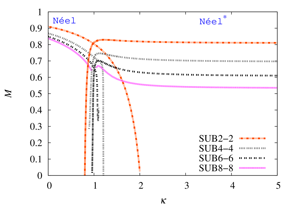
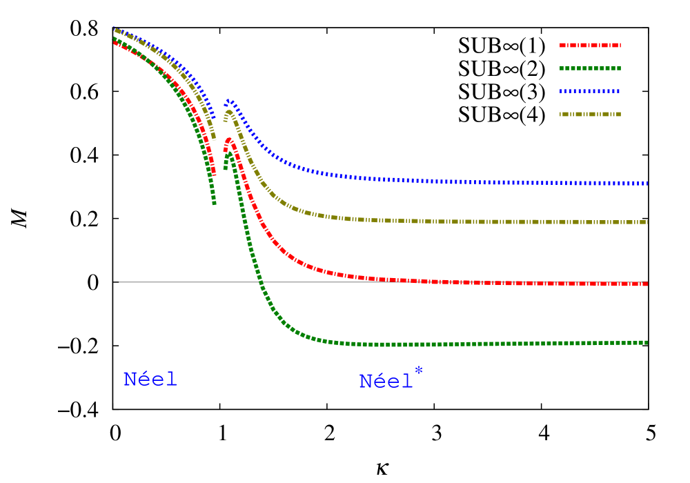
Figure 3: CCM results for the GS magnetic order parameter, $M$, as a function of the frustration parameter, $\kappa\equiv J_{2}/J_{1}$, for the spin-1 $J_{1}$–$J_{2}$ Heisenberg antiferromagnet (with $J_{1}>0$) on the checkerboard lattice. (a) The results for the SUB$n$–$n$ approximations with $n=\{2,4,6,8\}$ based on the Néel state (left curves) and Néel^∗ state (right curves) as the respective CCM model state. (b) The corresponding SUB$\infty(k)$ extrapolations: those with $k=\{1,2\}$ use the extrapolation scheme of Eq. (9), while those with $k=\{3,4\}$ use the extrapolation scheme of Eq. (8), in both cases with the respective SUB$n$–$n$ data sets: $k=\{1,3\}$, $n=\{2,4,6,8\}$; and $k=\{2,4\}$, $n=\{4,6,8\}$.

Firstly, in Fig. 3(a) we show the “raw” SUB$n$–$n$ results based on both the Néel state (left curves) and Néel^∗ state (right curves) used as the CCM model state. We note that the plus sign ($+$) symbols shown in Fig. 2 for the corresponding energy results correspond precisely to the respective points in Fig. 3(a) at which $M$ passes through zero. One sees clearly that in the vicinity of $\kappa=1$, the SUB$n$–$n$ curves for $M$ become increasingly steep as $n$ increases in value, thereby also demonstrating why we find increased difficulty in obtaining solutions in this region, which is also close to the corresponding termination points discussed previously. The raw SUB$n$–$n$ results show very clearly the existence of a phase transition with a QCP at or very close to $\kappa=1$, just as did the corresponding results for the GS energy shown in Fig. 2.

In Fig. 3(b) we also show the extrapolations of the results in Fig. 3(a), based on both the extrapolation schemes of Eqs. (8) and (9), and using each of the SUB$n$–$n$ data sets $n=\{2,4,6,8\}$ and $n=\{4,6,8\}$ in the two cases, for completeness and the sake of comparison. As we noted earlier, fits to each data set for $M$ for both model states used, of the form of Eq. (10), can also be performed to estimate the leading exponent and hence to determine which (if either) of the two forms of Eqs. (8) or (9) is appropriate in particular cases. We refer the interested reader to Ref. [88], for example, for a fuller description of the procedure. Based on such fits and much prior experience, the extrapolation scheme of Eq. (8) is now clearly indicated for our Néel-state results over most of the range of values of $\kappa$ for which solutions exist, except very near the point $\kappa=1$ where the extrapolation scheme of Eq. (9) becomes validated.

In particular, the use of Eq. (8) is clearly indicated at the point $\kappa=0$, corresponding to the special limiting case of the square-lattice HAFM. Our corresponding extrapolated results for the GS magnetic order parameter for the spin-1 square-lattice HAFM, using Eq. (8), are $M(\kappa=0)\approx 0.796$ based on SUB$n$–$n$ results with $n=\{4,6,8\}$, and $M(\kappa=0)\approx 0.798$ with $n=\{2,4,6,8\}$. Once again, these are in very good agreement with such independent results as $M(\kappa=0)\approx 0.804$ based on SWT-3 calculations [108] and $M(\kappa=0)=0.8039(4)$ from linked-cluster SE calculations [109]. Our current results are also in complete accord with previous CCM estimates [76, 79] discussed above in connection with the corresponding results for the GS energy.

We note from Fig. 3(a) that the SUB$n$–$n$ results based on the Néel state as CCM model state converge (with increasing values of $n$) much faster than those for the Néel^∗ state, which is fully consistent with a smaller value of the leading exponent $\nu$ in the scaling law for the latter results than for the former, over most of their respective ranges of existence. In this case, as explained before, the extrapolation scheme of Eq. (9), which has been validated by much prior experience, is found to be appropriate here too. The corresponding extrapolations based on the two data sets $n=\{2,4,6,8\}$ and $n=\{4,6,8\}$, shown in Fig. 3(b), now differ somewhat from each other. There are two reasons that come immediately to mind as possible explanations for this difference. The first is that the inclusion of the results with $n=2$ might bias the results somewhat, in view of them being rather far from the $n\rightarrow\infty$ limit. For this reason we usually prefer to exclude data with $n=2$. Another argument for doing so in general for square lattices is that since the basic square plaquette is an important structural element of models on the square lattice, approximations with $n\geq 4$ are preferred a priori. However, since we employ here SUB$n$–$n$ approximations based on the checkerboard geometry rather than the square-lattice geometry, such an argument loses much of its validity. By contrast, a second reason for the difference in extrapolations based on the two data sets shown is that 3-parameter fits based on only 3 inputs are inherently less stable than those based on 4 or more inputs, and for that reason we generally argue for fits of the latter type. Clearly, the above two arguments are in conflict over whether or not it is better to include or exclude the SUB2-2 results in our fits. From both Figs. 2 and 3(b) we observe that the fits are, nonetheless, remarkably similar in both cases for each of the GS quantities $E/N$ and $M$, with the single exception of results for $M$ in the region $\kappa\gtrsim 1$.

Despite the above caveat, it is abundantly clear that all of the results for $M$ in Figs. 3(a) and 3(b) point very strongly to a quantum phase transition at the same value $\kappa_{c_{1}}\approx 1.00\pm 0.01$ as indicated by the GS energy results in Fig. 2. It is clear too that the transition there is a very sharp one. The more likely scenario, based on these results, is of a continuous (but very steep or sharp) second-order transition at which $M\rightarrow 0$ on both sides of the transition. Clearly, however, we cannot exclude a weak first-order transition either in which $M$ approaches the same small (but nonzero) value on both sides of the transition or in which $M\rightarrow 0$ continuously on one side (likely the Néel side) and then discontinuously jumps to a small (but nonzero) value on the other (most likely, Néel^∗) side.

We turn finally to the results of $M$ in Fig. 3(b) based on the Néel^∗ state in the region $\kappa>1$. As indicated above the appropriate extrapolations in this region should be based on Eq. (9), and hence the relevant curves are those labelled SUB$\infty$(1) and SUB$\infty$(2). Conflicting reasons have already been discussed with regard to which of these two extrapolations to prefer, and it is hard to make an a priori decision on this basis. Nevertheless, we may also appeal to the known result that the spin-1 1D Haldane chain has $M=0$. Since this is precisely our limiting case $\kappa\rightarrow\infty$, on this basis the extrapolation curve SUB$\infty$(1) is clearly preferred, since it gives this result within very small errors.

What is clear from Fig. 3(b), however, is that whether we use the SUB$\infty$(1) or SUB$\infty$(2) result, there is clear evidence that Néel^∗ order is present only over a range of values of $\kappa_{c_{1}}<\kappa<\kappa_{c_{2}}$ of the frustration parameter. The SUB$\infty(2)$ curve shows $M<0$ in this case for $\kappa>\kappa_{c_{2}}\approx 1.4$ whereas the SUB$\infty(1)$ curve shows the more physical result that $M=0$ (within very small errors) for $\kappa>\kappa_{c_{2}}\approx 2.5$. The existence of this finite region of stable Néel^∗ order is quite different both from the $s=\frac{1}{2}$ version of the model (for which Néel^∗ order exists nowhere as a stable GS phase) and the classical ($s\rightarrow\infty$) version (for which it co-exists with an infinite family of states with AFM ordering along crossed $J_{2}$-coupled chains as the stable GS phase for all values $\kappa>\kappa_{{\rm cl}}=1$).

In Sec. 5 we summarize our results and compare further the present $s=1$ model with its $s=\frac{1}{2}$ and classical ($s\rightarrow\infty$) counterparts.

5 Discussion and summary

In this paper we have investigated the GS properties and GS ($T=0$) phase structure of the frustrated spin-1 AFM $J_{1}$–$J_{2}$ model (with $J_{1}>0,J_{2}\equiv\kappa J_{1}>0$) on the checkerboard lattice. To do so we have employed the CCM in the hierarchical SUB$n$–$n$ approximation scheme carried out to orders $n\leq 8$. As CCM model states we have employed two quasiclassical states, namely the Néel state and the Néel^∗ state. The former is the unique GS phase for $\kappa<\kappa_{{\rm cl}}=1$ for the classical version of the model, while the latter is one of an infinitely degenerate family of classical GS phases for $\kappa>\kappa_{{\rm cl}}=1$.

We find that for the $s=1$ model the GS phase is an AFM Néel-ordered state for $\kappa<\kappa_{c_{1}}$, at which point the staggered Néel magnetization vanishes. Our best estimate for this lower QCP is $\kappa_{c_{1}}\approx 1.00\pm 0.01$. On the one hand this value seems to concur with the classical value. On the other hand it is quite different from the $s=\frac{1}{2}$ value of $\kappa_{c}^{1}\approx 0.80\pm 0.01$, found previously [83].

In the classical version of the model the transition at $\kappa_{{\rm cl}}=1$ is a direct first-order one (with a discontinuity in the slope, $dE$/$d\kappa$, of the GS energy there). We find for the $s=1$ model that the corresponding transition at $\kappa_{c_{1}}$ is considerably “softened,” with the most likely scenario being that the transition is now a continuous (second-order) one, although we cannot on the available evidence rule out a weak first-order one. All of our evidence is that, as in the classical model, the transition at $\kappa_{c_{1}}$ is a direct one to a GS phase with another quasiclassical form of AFM ordering. We find zero evidence of any intermediate phase, and we can positively exclude such a phase except for a very narrow region around $\kappa_{c_{1}}$. If any such intermediate phase does exist (which we doubt on the present evidence), it can do so only over a tiny region confined to the range $0.99\lesssim\kappa\lesssim 1.01$. Similarly, if present at all, any region of coexistence of Néel and Néel^∗ ordering is restricted by our results to a correspondingly narrow range.

In the classical checkerboard model the Néel ordering that exists for $\kappa<\kappa_{{\rm cl}}=1$ gives way for all $\kappa>\kappa_{{\rm cl}}$ to an infinitely degenerate family of GS phases characterized by AFM ordering along the (crossed) $J_{2}$ chains. In the quasiclassical limit (where one works to leading order in $1/s$) it has been shown [97] that quantum fluctuations select, by the order by disorder mechanism [49, 50], a fourfold family of collinear states from among all other classically degenerate states. These comprise the stripe-ordered and Néel^∗ states, both of which are doubly degenerate. In a previous CCM study of the $s=\frac{1}{2}$ version of the present checkerboard model, the Néel^∗ state was found to have lower energy than the stripe-ordered state, and other authors [102] have also found evidence in favour of the Néel^∗ state for this model. Consequently in the present analysis we have also been motivated to use the Néel^∗ state as a CCM model state to investigate the phase structure of the $s=1$ checkerboard model for $\kappa>\kappa_{c_{1}}$. Nevertheless, further work should be done in the future to investigate, for example, whether a quasiclassical striped state might lie lower in energy than the Néel^∗ state for the $s=1$ model.

We have found clear evidence that a Néel^∗ state with nonzero values of the order parameter exists for the $s=1$ case for values of the frustration parameter $\kappa_{c_{1}}<\kappa<\kappa_{c_{2}}\approx 2.0\pm 0.5$. This finding, perhaps the most striking of this study, differs from both the $s=\frac{1}{2}$ and $s\rightarrow\infty$ (classical) versions of the model. Firstly, for the $s=\frac{1}{2}$ model, the previous CCM study [83] found that the Néel^∗ state could not survive quantum fluctuations to form a stable GS phase for any values of $\kappa$. When used as a CCM model state, although solutions could be found for $\kappa>\kappa_{c}^{1}$, the calculated (i.e., extrapolated) value of its order parameter $M$ was found to be zero (or negative) everywhere. By contrast, for the $s=1$ case we find that when the Néel^∗ state is used as the CCM model state, the calculated value of $M$ is zero (or negative) only for $\kappa>\kappa_{c_{2}}$ ($>\kappa_{c_{1}}$). Secondly, by contrast with the classical checkerboard model, where stable nonzero Néel^∗ ordering exists for all values $\kappa>\kappa_{{\rm cl}}$, its $s=1$ counterpart exists only over a finite range of values of $\kappa$.

The question thus remains as to what is the stable GS phase of the $s=1$ checkerboard model for $\kappa>\kappa_{c_{2}}$. We note that for its $s=\frac{1}{2}$ counterpart, the previous CCM study [83] found a PVBC-ordered phase for $\kappa_{c}^{1}<\kappa<\kappa_{c}^{2}\approx 1.22\pm 0.02$, which then gave way to a CDVBC-ordered phase for all $\kappa>\kappa_{c}^{2}$. We have also performed very preliminary calculations (which we will report on, more fully, elsewhere) for these phases for the $s=1$ model, using the same CCM technique as reported previously [83] for the $s=\frac{1}{2}$ case. Very interestingly, the evidence so far is that for all values $\kappa>\kappa_{c_{2}}$ the GS phase of the $s=1$ model seems to take PVBC ordering. Again, if this result stands up to further scrutiny, the $s=1$ model will again show distinct differences to both its $s=\frac{1}{2}$ and $s\rightarrow\infty$ counterparts.

Finally, we make some brief remarks regarding the order of the various quantum phase transitions exhibited by the checkerboard model, and in particular whether specific transitions are allowed to be continuous. Although a general renormalization group theory approach to continuous critical phenomena itself places only rather weak constraints on the existence of a continuous phase transition between any two quantum phases, the traditional (and conventional) Landau-Ginzburg-Wilson (LGW) approach [111, 112] places stricter criteria. In a nutshell LGW theory places as a necessary condition on a continuous transition from a phase $\mathcal{P}_{1}$ to a phase $\mathcal{P}_{2}$ that the symmetry group of phase $\mathcal{P}_{2}$ is a subgroup of that $\mathcal{P}_{1}$ [111]. Physically, the order parameter of some mode of phase $\mathcal{P}_{1}$ goes to zero at the transition as the mode becomes soft and macroscopic condensation into it hence occurs, with a consequent symmetry reduction.

A detailed analysis and description of the various LGW-allowed continuous phase transitions for the checkerboard model has been given elsewhere [102]. In particular it is shown explicitly that the symmetry group of the Néel^∗ state is a subgroup of that of the PVBC state. Hence, our tentative identification of the QCP at $\kappa_{c_{2}}$ in the $s=1$ checkerboard model as being between states with Néel^∗ and PVBC order, would be LGW-allowed as a continuous transition, and it will be interesting to examine the order of the transition in more detail. By contrast, it is not difficult to show (and see, e.g., Ref. [102] for explicit details) that the Néel^∗ and CDVBC states break different symmetries of the checkerboard lattice (and hence of the Hamiltonian), so that the symmetry group of neither state is a subgroup of the other. Hence, any continuous phase transition between states with Néel^∗ and CDVBC ordering would be LGW-forbidden. In such a case the most likely scenarios would be either a direct first-order transition or one that involves an intermediate coexistence phase with intermediate ordering and bond modulation. Reference [102] describes the possible properties of such a coexistence phase and the nature of the symmetry breakings at the two transition points from it into each of the pure phases.

The nature of the QCP at $\kappa_{c}^{2}$ in the $s=\frac{1}{2}$ model is also more open than that at $\kappa_{c_{2}}$ in the $s=1$ model. Thus, again, while both the CDVBC and PVBC phases are doubly degenerate (and can thus be described via Ising order parameters), it is easy to see that they have distinct symmetries [102]. Thus, again, neither state has a symmetry group which is a subgroup of that of the other, and a continuous transition between them is LGW-forbidden.

Lastly, we note too that the transitions at $\kappa_{c}^{1}$ in the $s=\frac{1}{2}$ model and at $\kappa_{c_{1}}$ in the $s=1$ model, from the Néel phase to, respectively, the PVBC phase (for $s=\frac{1}{2}$) and the Néel^∗ phase (for $s=1$) are both also LGW-forbidden as continuous transitions. Thus, for example, the Néel^∗ (and PVBC) phases both have rotations of $\frac{1}{2}\pi$ about the centre of any square plaquette containing four parallel spins as symmetries, which are not shared with the Néel phase. Hence, if the transition at $\kappa_{c_{1}}$ for the present $s=1$ model is indeed continuous, as seems possible from our results, its nature has to be sought outside the conventional LGW paradigm. One such possibility, which takes us too far afield to study further here however, is via the deconfinement scenario [113].

In conclusion, the $s=1$ checkerboard model has been shown to exhibit some very interesting features of its GS ($T=0$) phase diagram that are qualitatively different to those of both its $s=\frac{1}{2}$ and $s\rightarrow\infty$ (classical) counterparts. In future work we intend both to investigate the relative stabilities of the striped and Néel^∗ GS phases in the intermediate regime $\kappa_{c_{1}}<\kappa<\kappa_{c_{2}}$, and to perform a rigorous study of the stability of possible phases with VBC order, particularly those with PVBC and CDVBC ordering, in the regime $\kappa>\kappa_{c_{2}}$.

References

References

- [1] Haldane F D M 1983 Phys. Rev. Lett. 50 1153; Haldane F D M 1983 Phys. Lett. A 93 464
- [2] Steiner M, Kakurai K, Kjems J K, Petitgrand D and Pynn R 1987 J. Appl. Phys. 61 3953
- [3] Daniel J and Regnault L P 1993 Solid State Commun. 86 409
- [4] Dorner B, Visser D, Steigenberger U, Kakurai K and Steiner M 1988 Z. Phys. B 72 487
- [5] Renard J P, Verdaguer M, Regnault L P, Erkelens W A C and Rossat-Mignod J 1988 J. Appl. Phys. 63 3538
- [6] Orendáč M, Orendáčová A, Černák J, Feher A, Signore P J C, Meisel M W, Merah S and Verdaguer M 1995 Phys. Rev. B 52 3435
- [7] Zapf V S, Zocco D, Hansen B R, Jaime M, Harrison N, Batista C D, Kenzelmann M, Niedermayer C, Lacerda A and Paduan-Filho A 2006 Phys. Rev. Lett. 96 077204
- [8] Birgeneau R J, Skalyo J Jr. and Shirane G 1970 J. Appl. Phys. 41 1303
- [9] Nakatsuji S, Nambu Y, Tonomura H, Sakai O, Jonas S, Broholm C, Tsunetsugu H, Qiu Y M and Maeno Y 2005 Science 309 1697
- [10] Läuchli A, Mila F and Penc K 2006 Phys. Rev. Lett. 97 087205
- [11] Tsunetsugu H and Arikawa M 2006 J. Phys. Soc. Japan 75 083701
- [12] Bhattacharjee S, Shenoy V B and Senthil T 2006, Phys. Rev. B 74 092406
- [13] Kamihara Y, Watanabe T, Hirano M and Hosono H 2008 J. Am. Chem. Soc. 130 3296
- [14] Ma F, Lu Z-Y and Xiang T 2008 Phys. Rev. B 78 224517
- [15] Si Q and Abrahams E 2008 Phys. Rev. Lett. 101 076401
- [16] Chandra P and Doucot B 1988 Phys. Rev. B 38 9335
- [17] Gelfand M P, Singh R R P and Huse D A 1989 Phys. Rev. B 40 10801
- [18] Dagotto E and Moreo A 1989 Phys. Rev. Lett. 63 2148
- [19] Sachdev S and Bhatt R 1990 Phys. Rev. B 41 9323
- [20] Chubukov A V and Jolicoeur Th 1991 Phys. Rev. B 44 12050
- [21] Read N and Sachdev S 1991 Phys. Rev. Lett. 66 1773
- [22] Schulz H J and Ziman T A L 1992 Europhys. Lett. 18 355
- [23] Richter J 1993 Phys. Rev. B 47 5794
- [24] Richter J, Ivanov N B and Retzlaff K 1994 Europhys. Lett. 25 545
- [25] Oitmaa J and Weihong Z 1996 Phys. Rev. B 54 3022
- [26] Schulz H J, Ziman T A L and Poilblanc D 1996 J. Physique I 6 675
- [27] Zhitomirsky M E and Ueda K 1996 Phys. Rev. B 54 9007
- [28] Bishop R F, Farnell D J J and Parkinson J B 1998 Phys. Rev. B 58 6394
- [29] Singh R R P, Weihong Z, Hamer C J and Oitmaa J 1999 Phys. Rev. B 60 7278
- [30] Kotov V N, Oitmaa J, Sushkov O P and Weihong Z 1999 Phys. Rev. B 60 14613
- [31] Capriotti L and Sorella S 2000 Phys. Rev. Lett. 84 3173
- [32] Capriotti L, Becca F, Parola A and Sorella S 2001 Phys. Rev. Lett. 87 097201
- [33] Takano K, Kito Y, Ono Y and Sano K 2003 Phys. Rev. Lett. 91 197202
- [34] Roscilde T, Feiguin A, Chernyshev A L, Liu S and Haas S 2004 Phys. Rev. Lett. 93 017203
- [35] Sirker J, Weihong Z, Sushkov O P and Oitmaa J 2006 Phys. Rev. B 73 184420
- [36] Mambrini M, Läuchli A, Poiblanc D and Mila F 2006 Phys. Rev. B 74 144422
- [37] Schmalfuß D, Darradi R, Richter J, Schulenburg J and Ihle D 2006 Phys. Rev. Lett. 97 157201
- [38] Darradi R, Derzhko O, Zinke R, Schulenburg J, Krüger S E and Richter J 2008 Phys. Rev. B 78 214415
- [39] Ralko A, Mambrini M and Poiblanc D 2009 Phys. Rev. B 80 184427
- [40] Richter J and Schulenburg J 2010 Eur. Phys. J. B 73 117
- [41] Reuther J, Wölfle P, Darradi R, Brenig W, Arlego M and Richter J 2011 Phys. Rev. B 83 064416
- [42] Yu J-F and Kao Y-J 2012 Phys. Rev. B 85 094407
- [43] Götze O, Krüger S E, Fleck F, Schulenburg J and Richter J 2012 Phys. Rev. B 85 224424
- [44] Jiang H-C, Yao H and Balents L 2012 Phys. Rev. B 86 024424
- [45] Mezzacapo F 2012 Phys. Rev. B 86 045115
- [46] Li T, Becca F, Hu W and Sorella S 2012 Phys. Rev. B 86 075111
- [47] Wang L, Poilblanc D, Gu Z-C, Wen X-G and Verstraete F 2013 Phys. Rev. Lett. 111 037202
- [48] Hu W-J, Becca F, Parola A and Sorella S 2013 Phys. Rev. B 88 060402(R)
- [49] Villain J 1977 J. Physique 38 385; Villain J, Bidaux R, Carton J P and Conte R 1980 J. Physique 41 1263
- [50] Shender E 1982 Sov. Phys.-JETP 56 178
- [51] Bishop R F 1991 Theor. Chim. Acta 80 95
- [52] Bishop R F 1998 Microscopic Quantum Many-Body Theories and Their Applications (Springer Lecture Notes in Physics vol 510) ed J Navarro and A Polls (Berlin: Springer) p 1
- [53] Zeng C, Farnell D J J and Bishop R F 1998 J. Stat. Phys. 90 327
- [54] Farnell D J J and Bishop R F 2004 Quantum Magnetism (Springer Lecture Notes in Physics vol 645) ed U Schollwöck, J Richter, D J J Farnell and R F Bishop (Berlin: Springer) p 307
- [55] Roger M and Hetherington J H 1990 Phys. Rev. B 41 200
- [56] Bishop R F, Parkinson J B and Xian Y 1991 Phys. Rev. B 43 13782(R)
- [57] Bishop R F, Parkinson J B and Xian Y 1992 Phys. Rev. B 46 880
- [58] Bishop R F, Parkinson J B and Xian Y 1992 J. Phys.: Condens. Matter 4 5783
- [59] Bishop R F, Parkinson J B and Xian Y 1993 J. Phys.: Condens. Matter 5 9169
- [60] Zeng C, Staples I and Bishop R F 1996 Phys. Rev. B 53 9168
- [61] Bishop R F, Farnell D J J, Krüger S E, Parkinson J B, Richter J and Zeng C 2000 J. Phys.: Condens. Matter 12 6887
- [62] Krüger S E, Richter J, Schulenburg J, Farnell D J J and Bishop R F 2000 Phys. Rev. B 61 14607
- [63] Farnell D J J, Gernoth K A and Bishop R F 2001 Phys. Rev. B 64 172409
- [64] Farnell D J J, Bishop R F and Gernoth K A 2002 J. Stat. Phys. 108 401
- [65] Darradi R, Richter J and Farnell D J J 2005 Phys. Rev. B 72 104425
- [66] Farnell D J J and Bishop R F 2008 Int. J. Mod. Phys. B 22 3369
- [67] Bishop R F, Li P H Y, Darradi R, Schulenburg J and Richter J 2008 Phys. Rev. B 78 054412
- [68] Bishop R F, Li P H Y, Darradi R and Richter J 2008 J. Phys.: Condens. Matter 20 255251
- [69] Bishop R F, Li P H Y, Darradi R and Richter J 2008 Europhys. Lett. 83 47004
- [70] Bishop R F, Li P H Y, Darradi R, Richter J and Campbell C E 2008 J. Phys.: Condens. Matter 20 415213
- [71] Farnell D J J, Richter J, Zinke R and Bishop R F 2009 J. Stat. Phys. 135 175
- [72] Bishop R F, Li P H Y, Farnell D J J and Campbell C E 2009 Phys. Rev. B 79 174405
- [73] Richter J, Darradi R, Schulenburg J, Farnell D J J and Rosner H 2010 Phys. Rev. B 81 174429
- [74] Bishop R F, Li P H Y, Farnell D J J and Campbell C E 2010 Phys. Rev. B 82 024416
- [75] Bishop R F, Li P H Y, Farnell D J J and Campbell C E 2010 Phys. Rev. B 82 104406
- [76] Bishop R F and Li P H Y 2011 Eur. Phys. J. B 81 37
- [77] Farnell D J J, Bishop R F, Li P H Y, Richter J and Campbell C E 2011 Phys. Rev. B 84 012403
- [78] Götze O, Farnell D J J, Bishop R F, Li P H Y and Richter J 2011 Phys. Rev. B 84 224428
- [79] Bishop R F and Li P H Y 2012 Eur. Phys. J. B 85 25
- [80] Li P H Y, Bishop R F, Farnell D J J, Richter J and Campbell C E 2012 Phys. Rev. B 85 085115
- [81] Bishop R F, Li P H Y, Farnell D J J and Campbell C E 2012 J. Phys.: Condens. Matter 24 236002
- [82] Bishop R F and Li P H Y 2012 Phys. Rev. B 85 155135
- [83] Bishop R F, Li P H Y, Farnell D J J, Richter J and Campbell C E 2012 Phys. Rev. B 85 205122
- [84] Li P H Y, Bishop R F, Farnell D J J and Campbell C E 2012 Phys. Rev. B 86 144404
- [85] Li P H Y, Bishop R F, Campbell C E, Farnell D J J, Götze O and Richter J 2012 Phys. Rev. B 86 214403
- [86] Bishop R F, Li P H Y and Campbell C E 2013 J. Phys.: Condens. Matter 25 306002
- [87] Li P H Y, Bishop R F and Campbell C E 2013 Phys. Rev. B 88 144423
- [88] Bishop R F, Li P H Y and Campbell C E 2013 arXiv:1308.4573v2 [cond-mat.str-el]
- [89] Singh R R P, Starykh O A and Freitas P J 1998 J. Appl. Phys. 83 7387
- [90] Palmer S E and Chalker J T 2001 Phys. Rev. B 64 094412
- [91] Brenig W and Honecker A 2002 Phys. Rev. B 65 140407(R)
- [92] Canals B 2002 Phys. Rev. B 65 184408
- [93] Starykh O A, Singh R R P and Levine G C 2002 Phys. Rev. Lett. 88 167203
- [94] Sindzingre P, Fouet J-B and Lhuillier C 2002 Phys. Rev. B 66 174424
- [95] Fouet J-B, Mambrini M, Sindzingre P and Lhuillier C 2003 Phys. Rev. B 67 054411
- [96] Berg E, Altman E and Auerbach A 2003 Phys. Rev. Lett. 90 147204
- [97] Tchernyshyov O, Starykh O A, Moessner R and Abanov A G 2003 Phys. Rev. B 68 144422
- [98] Moessner R, Tchernyshyov O and Sondhi S L 2004 J. Stat. Phys. 116 755
- [99] Hermele M, Fisher M P A and Balents L 2004 Phys. Rev. B 69 064404
- [100] Brenig W and Grzeschik M 2004 Phys. Rev. B 69 064420
- [101] Bernier J S, Chung C H, Kim Y B and Sachdev S 2004 Phys. Rev. B 69 214427
- [102] Starykh O A, Furusaki A and Balents L 2005 Phys. Rev. B 72 094416
- [103] Schmidt H-J, Richter J and Moessner R 2006 J. Phys. A: Math. Gen. 39 10673
- [104] Arlego M and Brenig W 2007 Phys. Rev. B 75 024409; Arlego M and Brenig W 2009 Phys. Rev. B 80 099902(E)
- [105] Moukouri S 2008 Phys. Rev. B 77 052408
- [106] Chan Y-H, Han Y-J and Duan L-M 2011 Phys. Rev. B 84 224407
- [107] We use the program package CCCM of Farnell D J J and Schulenburg J, see http://www-e.uni-magdeburg.de/jschulen/ccm/index.html
- [108] Hamer C J, Zheng Weihong and Arndt P 1992 Phys. Rev. B 46 6276
- [109] Zheng Weihong, Oitmaa J and Hamer C J 1991 Phys. Rev. B 43 8321
- [110] White S R and Huse D A 1993 Phys. Rev. B 48 3844
- [111] Landau L D, Lifshitz E M and Pitaevskii L P 1980 Statistical Physics (3rd ed) (Oxford: Butterworth-Heinemann)
- [112] Wilson K G and Kogut J 1974 Phys. Rep. 12 75
- [113] Senthil T, Vishwanath A, Balents L, Sachdev S and Fisher M P A 2004 Science 303 1490